ISC: an RADI-type method for stochastic continuous-time algebraic Riccati equations

Abstract

In this paper, we propose an RADI-type method for large-scale stochastic continuous-time algebraic Riccati equations with sparse and low-rank structures. The so-called ISC method is developed by using the Incorporation idea together with different Shifts to accelerate the convergence and Compressions to reduce the storage and complexity. Numerical experiments are given to show its efficiency.

Key words. RADI, algebraic Riccati equations, stochastic control, linear-quadratic optimal control, left semi-tensor product.

AMS subject classifications. 65F45, 15A24

1 Introduction

Consider the stochastic continuous-time algebraic Riccati equations (SCAREs)

$$\begin{multlined}Q+A_{{0}}^{\operatorname{T}}X+XA_{{0}}+\sum_{i=1}^{{r-1}}A_{i}^{\operatorname{T}}XA_{i}-(L+XB_{{0}}+\sum_{i=1}^{{r-1}}A_{i}^{\operatorname{T}}XB_{i})\cdot\\ \qquad\qquad\qquad(R+\sum_{i=1}^{{r-1}}B_{i}^{\operatorname{T}}XB_{i})^{-1}(L^{\operatorname{T}}+B_{{0}}^{\operatorname{T}}X+\sum_{i=1}^{{r-1}}B_{i}^{\operatorname{T}}XA_{i})=0,\end{multlined}Q+A_{{0}}^{\operatorname{T}}X+XA_{{0}}+\sum_{i=1}^{{r-1}}A_{i}^{\operatorname{T}}XA_{i}-(L+XB_{{0}}+\sum_{i=1}^{{r-1}}A_{i}^{\operatorname{T}}XB_{i})\cdot\\ \qquad\qquad\qquad(R+\sum_{i=1}^{{r-1}}B_{i}^{\operatorname{T}}XB_{i})^{-1}(L^{\operatorname{T}}+B_{{0}}^{\operatorname{T}}X+\sum_{i=1}^{{r-1}}B_{i}^{\operatorname{T}}XA_{i})=0,$$ (1.1)

where $A_{i}\in\mathbb{R}^{n\times n},B_{i}\in\mathbb{R}^{n\times m}$ for $i=0,1,\cdots,r-1$, $R\in\mathbb{R}^{m\times m}$ is positive definite and $L\in\mathbb{R}^{n\times m}$ with $\begin{bmatrix}Q&L\\ L^{\operatorname{T}}&R\end{bmatrix}$ positive semi-definite. Here $r-1$ is the number of stochastic processes involved in the stochastic systems dealt with, and it is easy to check that for the case $r=1$ the SCAREs degenerate to the classical continuous-time algebraic Riccati equations (CAREs):

$$Q+A^{\operatorname{T}}X+XA-(L+XB)R^{-1}(L^{\operatorname{T}}+B^{\operatorname{T}}X)=0.$$

Due to the complicated forms, one may realize the SCAREs would be much more difficult to analyze and solve, unlike the situation for the CAREs that people have developed rich theoretical results and numerical methods. Readers interested in CAREs are referred to [26, 25, 22, 4, 20, 3] to obtain an overview for both theories and algorithms. A few literature, e.g., [10, 13], discuss the stochastic linear systems and the induced SCAREs theoretically. The existing methods to solve SCAREs include Newton’s method [10, 9], modified Newton’s method [17, 23, 8], Newton’s method with generalized Lyapunov/Stein equation solver [14, 24, 30], comparison theorem based method [15, 16], LMI’s (linear matrix inequality) method [28, 21], and homotopy method [32].

In this paper, we focus on a special case that $A_{i}$ are large-scale and sparse, and $B_{i}$ and $Q-LR^{-1}L^{T}$ are low-rank. With the help of the algebraic structures discovered by the authors [19], motivated by the relation illustrated in [18] between the algebraic structure and the efficient RADI method [1] for CAREs, we are successful to propose an RADI-type method to solve large-scale SCAREs, named Incorporation with Shift and Compression (ISC).

The rest of the paper is organized as follows. First some notation and a brief description on SCAREs are given immediately. Then we begin to discuss the idea of incorporation (a.k.a. defect correction) performing on SCAREs and a low-rank expression of the residual generated by a chosen approximation in Section 2, which is only possible under the discovered algebraic structure. This derives a prototype of an RADI-type method. Afterwards efforts are made to convert it practical in Section 3. Numerical experiments and some related discussions are given in Section 4. Some concluding remarks in Section 5 end the paper.

1.1 Notation

In this paper, ${\mathbb{R}}^{n\times m}$ is the set of all $n\times m$ real matrices, ${\mathbb{R}}^{n}={\mathbb{R}}^{n\times 1}$, and ${\mathbb{R}}={\mathbb{R}}^{1}$. $I_{n}$ (or simply $I$ if its dimension is clear from the context) is the $n\times n$ identity matrix. Given a matrix $X$, $X^{T}$ is its transpose and $X^{-\operatorname{T}}=(X^{-1})^{\operatorname{T}}$. For a symmetric matrix $X$, $X\succ 0$ ($X\succeq 0$) indicates its positive (semi-)definiteness, and $X\prec 0$ ($X\preceq 0$) if $-X\succ 0$ ($-X\succeq 0$).

The left semi-tensor product, first defined in 2001 [5], has many applications in system and control theory, such as Boolean networks [7] and electrical systems [31]. Please seek more information in the monograph [6].

By $A\otimes B$ denote the Kronecker product of the matrices $A$ and $B$. For $A\in\mathbb{R}^{m\times n},B\in\mathbb{R}^{p\times q}$, define the left semi-tensor product of $A$ and $B$:

$$A\ltimes B:=\begin{dcases*}(A\otimes I_{p/n})B&if $n\mid p$,\\ A(B\otimes I_{n/p})&if $p\mid n$.\end{dcases*}$$

Clearly $A\ltimes B=AB$ if $n=p$. This product satisfies:

• $(A\ltimes B)\ltimes C=A\ltimes(B\ltimes C)$ (so the parenthesis can be omitted);

• $(A+B)\ltimes C=A\ltimes C+B\ltimes C,A\ltimes(B+C)=A\ltimes B+A\ltimes C$;

• $(A\ltimes B)^{-1}=B^{-1}\ltimes A^{-1}$;

• $(A\ltimes B)^{\operatorname{T}}=B^{\operatorname{T}}\ltimes A^{\operatorname{T}}$;

• $\!\!\begin{bmatrix}A_{11}&\!A_{12}\\ A_{21}&\!A_{22}\\ \end{bmatrix}\!\ltimes\!\begin{bmatrix}B_{11}&\!B_{12}\\ B_{21}&\!B_{22}\\ \end{bmatrix}\!\!=\!\!\begin{bmatrix}A_{11}\ltimes B_{11}+A_{12}\ltimes B_{21}&\!A_{11}\ltimes B_{12}+A_{12}\ltimes B_{22}\\ A_{21}\ltimes B_{11}+A_{22}\ltimes B_{21}&\!A_{21}\ltimes B_{12}+A_{22}\ltimes B_{22}\\ \end{bmatrix}\!$.

The left semi-tensor product, which satisfies the same arithmetic laws as the classical matrix product, can be treated as the matrix product in the following sections. Briefly, we write $A^{\ltimes k}=\underbrace{A\ltimes A\ltimes\dots\ltimes A}_{k}$.

Some easy identities are given:

$$U\ltimes(I+V\ltimes U)=(I+U\ltimes V)\ltimes U,\qquad U\ltimes(I+V\ltimes U)^{-1}=(I+U\ltimes V)^{-1}\ltimes U.$$ (1.2)

Here is the Sherman-Morrison-Woodbury formula:

$$(M+U\ltimes D\ltimes V)^{-1}=M^{-1}-M^{-1}\ltimes U\ltimes(D^{-1}+V\ltimes M^{-1}\ltimes U)^{-1}\ltimes V\ltimes M^{-1}.$$ (1.3)

The inverse sign in 1.2 and 1.3 indicates invertibility.

1.2 Basics on SCAREs

The SCARE 1.1 arises from the stochastic time-invariant control system in continuous-time subject to multiplicative white noise, whose dynamics is described as below:

$$\operatorname{d\!}x(t) =A_{0}x(t)\operatorname{d\!}t+B_{0}u(t)\operatorname{d\!}t+\sum_{i=1}^{r-1}(A_{i}x(t)+B_{i}u(t))\operatorname{d\!}w_{i}(t),$$ (1.4)

$$z(t) ={C_{z}}x(t)+{D_{z}}u(t),$$

in which $x(t),u(t)$ and $z(t)$ are state, input, measurement, respectively, and $w(t)=\begin{bmatrix}w_{1}(t)&\cdots&w_{r-1}(t)\end{bmatrix}^{\operatorname{T}}$ is a standard Wiener process satisfying that each $w_{i}(t)$ is a standard Brownian motion and the $\sigma$-algebras $\sigma\left(w_{i}(t),t\in[t_{0},\infty)\right),i=1,\dots,r-1$ are independent [13]. Considering the cost functional with respect to the control $u(t)$ with the given initial $x_{0}$:

$$J(t_{0},x_{0};u)=\operatorname{\mathrm{E}}\left\{\int_{t_{0}}^{\infty}\begin{bmatrix}x_{t_{0},x_{0};u}(t)\\ u(t)\end{bmatrix}^{\operatorname{T}}\begin{bmatrix}Q&L\\ L^{\operatorname{T}}&R\end{bmatrix}\begin{bmatrix}x_{t_{0},x_{0};u}(t)\\ u(t)\end{bmatrix}\operatorname{d\!}t\right\},$$ (1.5)

where $x_{t_{0},x_{0};u}(t)$ is the solution of the system 1.4 corresponding to the input $u(t)$ with the initial $x_{t_{0},x_{0};u}(t_{0})=x_{0}$, one goal in stochastic control is to minimize the cost functional 1.5 and compute an optimal control. Such an optimization problem is also called the first linear-quadratic optimization problem [13, Section 6.2].

Assume the following conditions hold throughout this paper:

1. $R\succ 0$;

2. the pair $(\{A_{i}\}_{i=0}^{r-1},\{B_{i}\}_{i=0}^{r-1})$ is stabilizable, i.e., there exists $F\in\mathbb{R}^{m\times n}$ such that the linear differential equation

   $$\frac{\operatorname{d\!}}{\operatorname{d\!}t}S(t)=\mathscr{L}_{F}S(t):=(A_{0}+B_{0}F)S+S(A_{0}+B_{0}F)^{\operatorname{T}}+\sum_{i=1}^{r-1}(A_{i}+B_{i}F)S(A_{i}+B_{i}F)^{\operatorname{T}}$$

   is exponentially stable, or equivalently, the evolution operator $\mathrm{e}^{\mathscr{L}_{F}(t-t_{0})}$ is stable with $\mathrm{e}^{\mathscr{L}_{F}t}=\sum_{k=0}^{\infty}\frac{\mathscr{L}_{F}^{k}t^{k}}{k!}$; and

3. the pair $(\{A_{i}\}_{i=0}^{{r-1}},C)$ is detectable with $C^{\operatorname{T}}C=Q-LR^{-1}L^{\operatorname{T}}$, or equivalently, $(\{A_{i}^{\operatorname{T}}\}_{i=0}^{r-1},\{C_{i}^{\operatorname{T}}\}_{i=0}^{r-1})$ is stabilizable with $C_{0}=C$ and $C_{i}=0$ for $i=1,\cdots,r-1$.

It is known that if the assumption above holds, then 1.1 has a unique positive semi-definite stabilizing solution $X_{\star}$, see, e.g., [13, Theorem 5.6.15]. Here, $X$ is a stabilizing solution if the system $(A_{0}+B_{0}F_{X},A_{1}+B_{1}F_{X},\cdots,A_{r-1}+B_{r-1}F_{X})$ is stable with

$$F_{X}=-(R+\sum_{i=1}^{r-1}B_{i}^{\operatorname{T}}XB_{i})^{-1}(L^{\operatorname{T}}+B_{0}^{\operatorname{T}}X+\sum_{i=1}^{r-1}B_{i}^{\operatorname{T}}XA_{i}),$$ (1.6)

or equivalently, $\mathscr{L}_{F_{X}}$ is exponentially stable with the associated $F_{\star}=F_{X_{\star}}$ taking the feedback control specified in 1.6 with $X=X_{\star}$. In fact, $X_{\star}$ is a stabilizing solution if and only if the zero equilibrium of the closed-loop system

$$\operatorname{d\!}x(t)=(A_{0}+B_{0}F_{\star})x(t)\operatorname{d\!}t+\sum_{i=1}^{r-1}(A_{i}+B_{i}F_{\star})x(t)\operatorname{d\!}w_{i}(t)$$ (1.7)

is strongly exponentially stable in the mean square [12, Remark 5.11], where $F_{\star}=F_{X_{\star}}$ is as in 1.6 with $X=X_{\star}$. Furthermore, the cost functional 1.5 has an optimal control $u(t)=F_{\star}x_{t_{0},x_{0}}(t)$ where $x_{t_{0},x_{0}}(t)$ is the solution to the corresponding closed-loop system 1.7.

Following [19], 1.1 can be reformulated as the following equivalent standard form:

$$\begin{multlined}C^{\operatorname{T}}C+A^{\operatorname{T}}X+XA+\widehat{A}^{\operatorname{T}}\ltimes X\ltimes\widehat{A}\\ -(XB+\widehat{A}^{\operatorname{T}}\ltimes X\ltimes\widehat{B})(I+\widehat{B}^{\operatorname{T}}\ltimes X\ltimes\widehat{B})^{-1}(B^{\operatorname{T}}X+\widehat{B}^{\operatorname{T}}\ltimes X\ltimes\widehat{A})=0,\end{multlined}C^{\operatorname{T}}C+A^{\operatorname{T}}X+XA+\widehat{A}^{\operatorname{T}}\ltimes X\ltimes\widehat{A}\\ -(XB+\widehat{A}^{\operatorname{T}}\ltimes X\ltimes\widehat{B})(I+\widehat{B}^{\operatorname{T}}\ltimes X\ltimes\widehat{B})^{-1}(B^{\operatorname{T}}X+\widehat{B}^{\operatorname{T}}\ltimes X\ltimes\widehat{A})=0,$$ (1.8)

where

$$A=A_{{0}}-B_{{0}}R^{-1}L^{\operatorname{T}}\in\mathbb{R}^{n\times n},\qquad B=B_{{0}}R^{-1/2}\in\mathbb{R}^{n\times m},\qquad C\in\mathbb{R}^{l\times n},$$

$$\widehat{A}=\Pi\left(\begin{bmatrix}A_{1}\\ \vdots\\ A_{r-1}\end{bmatrix}-\begin{bmatrix}B_{1}\\ \vdots\\ B_{r-1}\end{bmatrix}R^{-1}L^{\operatorname{T}}\right)\in\mathbb{R}^{{(r-1)}n\times n},\qquad\widehat{B}=\Pi\begin{bmatrix}B_{1}\\ \vdots\\ B_{r-1}\end{bmatrix}R^{-1/2}\in\mathbb{R}^{{(r-1)}n\times m}$$

with $\Pi$ being the permutation satisfying $\Pi^{\operatorname{T}}(X\otimes I_{{r-1}})\Pi=I_{{r-1}}\otimes X$, and $R^{-1/2}=(R^{1/2})^{-1}$ satisfying $(R^{1/2})^{T}R^{1/2}=R$. With the new notations, the feedback control $F_{X}$ and the closed-loop matrix are reformulated as

$$F_{X} ={-R^{-1}L^{\operatorname{T}}+R^{-1/2}\widehat{F}_{X}},$$ (1.9)

$$\begin{bmatrix}A_{{0}}+B_{{0}}F_{X}\\ A_{1}+B_{1}F_{X}\\ \vdots\\ A_{r-1}+B_{r-1}F_{X}\end{bmatrix} =\begin{bmatrix}A\\ \Pi^{\operatorname{T}}\widehat{A}\end{bmatrix}+\begin{bmatrix}B\\ \Pi^{\operatorname{T}}\widehat{B}\end{bmatrix}{\widehat{F}_{X}},$$

where $\widehat{F}_{X}=-(I+\widehat{B}^{\operatorname{T}}\ltimes X\ltimes\widehat{B})^{-1}(XB+\widehat{A}^{\operatorname{T}}\ltimes X\ltimes\widehat{B})^{\operatorname{T}}$ is the feedback control of the standard form 1.8.

Besides, Item 2 is equivalent to

1. there exists $F\in\mathbb{R}^{m\times n}$ such that the adjoint of the operator $\mathrm{e}^{\mathscr{L}_{F}(t-t_{0})}$ is stable, namely $\mathrm{e}^{\mathscr{L}_{F}^{*}(t-t_{0})}$ is stable where

   $$\mathscr{L}_{F}^{*}\colon S\mapsto (A_{0}+B_{0}F)^{\operatorname{T}}S+S(A_{0}+B_{0}F)+\sum_{i=1}^{r-1}(A_{i}+B_{i}F)^{\operatorname{T}}S(A_{i}+B_{i}F)$$

   $$=(A+B\widehat{F})^{\operatorname{T}}S+S(A+B\widehat{F})+(\widehat{A}+\widehat{B}\widehat{F})^{\operatorname{T}}\ltimes S\ltimes(\widehat{A}+\widehat{B}\widehat{F}),$$

   where $\widehat{F}=(R^{-1/2})^{T}L^{\operatorname{T}}+R^{1/2}F$.

2 Incorporation and RADI-type method

Similarly to the relation between the CAREs and the discrete-time algebraic Riccati equations (DAREs), we can also transform SCAREs to stochastic discrete-time algebraic Riccati equations (SDAREs), shown in Lemma 2.1.

Lemma 2.1 ([19, Theorem 3.2]).

The SCARE 1.8 is equivalent to the following SDARE:

$$X=E_{\gamma}^{\operatorname{T}}\ltimes X\ltimes(I+G_{\gamma}\ltimes X)^{-1}\ltimes E_{\gamma}+H_{\gamma},$$ (2.1)

where

$$E_{\gamma} =\widetilde{\Pi}\begin{bmatrix}A_{\gamma}+2\gamma I_{n}+BY_{\gamma}^{\operatorname{T}}C\\ \sqrt{2\gamma}(\widehat{A}+\widehat{B}Y_{\gamma}^{\operatorname{T}}C)\end{bmatrix}(I_{n}+A_{\gamma}^{-1}BY_{\gamma}^{\operatorname{T}}C)^{-1}A_{\gamma}^{-1}\in\mathbb{R}^{rn\times n},$$ (2.2a)

$$H_{\gamma} =2\gamma A_{\gamma}^{-\operatorname{T}}C^{\operatorname{T}}(I_{l}+Y_{\gamma}Y_{\gamma}^{\operatorname{T}})^{-1}CA_{\gamma}^{-1}\succeq 0\in\mathbb{R}^{n\times n},$$ (2.2b)

$$G_{\gamma} =\widetilde{\Pi}\begin{bmatrix}\sqrt{2\gamma}A_{\gamma}^{-1}B\\ \widehat{A}A_{\gamma}^{-1}B-\widehat{B}\end{bmatrix}(I_{m}+Y_{\gamma}^{\operatorname{T}}Y_{\gamma})^{-1}\begin{bmatrix}\sqrt{2\gamma}A_{\gamma}^{-1}B\\ \widehat{A}A_{\gamma}^{-1}B-\widehat{B}\end{bmatrix}^{\operatorname{T}}\widetilde{\Pi}^{\operatorname{T}}\succeq 0\in\mathbb{R}^{rn\times rn},$$ (2.2c)

for proper $\gamma>0$. Here $A_{\gamma}=A-\gamma I,Y_{\gamma}=CA_{\gamma}^{-1}B$ and $\widetilde{\Pi}$ is a permutation satisfying $\begin{bmatrix}S&\\ &S\otimes I_{r-1}\end{bmatrix}=\widetilde{\Pi}^{\operatorname{T}}(S\otimes I_{r})\widetilde{\Pi}$ for any arbitrary $S\in\mathbb{R}^{n\times n}$.

Moreover, the SDARE 2.1 has a unique positive semi-definite stabilizing solution, which is also the unique stabilizing solution of the SCARE 1.8.

Inspired by Lemma 2.1 and the convergence of fixed point iterations [19, Theorem 2.1], one can compute an approximation for the unique stabilizing solution $X_{\star}$ by pursuing the following process:

$$X_{t+1}=\mathscr{D}_{\gamma}(X_{t})=E_{\gamma}^{\operatorname{T}}\ltimes X_{t}\ltimes(I+G_{\gamma}\ltimes X_{t})^{-1}\ltimes E_{\gamma}+H_{\gamma},\qquad X_{0}=0.$$ (2.3)

In this way, like the Toeplitz-structured closed form for the stabilizing solution to an SDARE [19, Theorem 2.2], we may also obtain that for the original SCARE, an analogue of [18, Theorem 8], which can be found in Appendix A.

However, it would be inapplicable and unfavorable due to its linear convergence, especially for cases that the approximation approaches near to the solution [4]. Like the discussion in [18, Section 4.2] for the CAREs, the fixed point iteration 2.3 can be used to derive an efficient RADI-type method under the philosophy of incorporation.

2.1 Residual and incorporation

Define the residual operator

$$\mathscr{C}(X) =\begin{multlined}C^{\operatorname{T}}C+A^{\operatorname{T}}X+XA+\widehat{A}^{\operatorname{T}}\ltimes X\ltimes\widehat{A}\\ -(XB+\widehat{A}^{\operatorname{T}}\ltimes X\ltimes\widehat{B})(I+\widehat{B}^{\operatorname{T}}\ltimes X\ltimes\widehat{B})^{-1}(B^{\operatorname{T}}X+\widehat{B}^{\operatorname{T}}\ltimes X\ltimes\widehat{A}),\end{multlined}C^{\operatorname{T}}C+A^{\operatorname{T}}X+XA+\widehat{A}^{\operatorname{T}}\ltimes X\ltimes\widehat{A}\\ -(XB+\widehat{A}^{\operatorname{T}}\ltimes X\ltimes\widehat{B})(I+\widehat{B}^{\operatorname{T}}\ltimes X\ltimes\widehat{B})^{-1}(B^{\operatorname{T}}X+\widehat{B}^{\operatorname{T}}\ltimes X\ltimes\widehat{A}),$$

and then the SCARE 1.8 is $\mathscr{C}(X)=0$.

The idea of the incorporation is: once an approximate solution $\widetilde{X}$ is obtained, writing the difference from the exact solution $X_{\star}$ as $\Delta=X_{\star}-\widetilde{X}$, the original equation $\mathscr{C}(X_{\star})=0$ can be transformed into a new equation $\mathscr{C}_{\widetilde{X}}(\Delta)=0$ that would probably be of the same type, which would be solved more efficiently. Moreover, this process can be repeated to obtain approximate solutions more and more accurate.

In the following, we show that the new equation $\mathscr{C}_{\widetilde{X}}(\Delta)=0$ is indeed of the same type, namely also an SCARE. As preparations, we calculate the difference of the residuals of symmetric matrices $X+\Delta$ and $X$:

$$\mathscr{C}(X+\Delta)-\mathscr{C}(X)$$

$$=\begin{multlined}A^{\operatorname{T}}\Delta+\Delta A+\widehat{A}^{\operatorname{T}}\ltimes\Delta\ltimes\widehat{A}+(XB+\widehat{A}^{\operatorname{T}}\ltimes X\ltimes\widehat{B})(I+\widehat{B}^{\operatorname{T}}\ltimes X\ltimes\widehat{B})^{-1}(XB+\widehat{A}^{\operatorname{T}}\ltimes X\ltimes\widehat{B})^{T}\\ -([X+\Delta]B+\widehat{A}^{\operatorname{T}}\ltimes[X+\Delta]\ltimes\widehat{B})(I+\widehat{B}^{\operatorname{T}}\ltimes[X+\Delta]\ltimes\widehat{B})^{-1}([X+\Delta]B+\widehat{A}^{\operatorname{T}}\ltimes[X+\Delta]\ltimes\widehat{B})^{T}.\end{multlined}A^{\operatorname{T}}\Delta+\Delta A+\widehat{A}^{\operatorname{T}}\ltimes\Delta\ltimes\widehat{A}+(XB+\widehat{A}^{\operatorname{T}}\ltimes X\ltimes\widehat{B})(I+\widehat{B}^{\operatorname{T}}\ltimes X\ltimes\widehat{B})^{-1}(XB+\widehat{A}^{\operatorname{T}}\ltimes X\ltimes\widehat{B})^{T}\\ -([X+\Delta]B+\widehat{A}^{\operatorname{T}}\ltimes[X+\Delta]\ltimes\widehat{B})(I+\widehat{B}^{\operatorname{T}}\ltimes[X+\Delta]\ltimes\widehat{B})^{-1}([X+\Delta]B+\widehat{A}^{\operatorname{T}}\ltimes[X+\Delta]\ltimes\widehat{B})^{T}.$$

Factorize $\widehat{B}^{\operatorname{T}}\ltimes X\ltimes\widehat{B}+I=:R_{X}=(R^{1/2}_{X})^{T}R^{1/2}_{X}$ and write

$$B_{X}=BR^{-1/2}_{X},\widehat{B}_{X}=\widehat{B}R^{-1/2}_{X},A_{X}=A-B_{X}L^{T}_{X},\widehat{A}_{X}=\widehat{A}-\widehat{B}_{X}L^{T}_{X},$$ (2.4)

where $R^{-1/2}_{X}=(R^{1/2}_{X})^{-1},L^{T}_{X}=B_{X}^{\operatorname{T}}X+\widehat{B}_{X}^{\operatorname{T}}\ltimes X\ltimes\widehat{A}$. Note that for $F_{X}$ in 1.6 with the standard form 1.8 (at the case $\widehat{F}=F$ in 1.9),

$$F_{X}=-R^{-1/2}_{X}L^{T}_{X},\qquad A_{X}=A+BF_{X},\widehat{A}_{X}=\widehat{A}+\widehat{B}F_{X}.$$

Then by 2.4

$$\mathscr{C}(X+\Delta)-\mathscr{C}(X)$$

$$=\begin{aligned} &A^{\operatorname{T}}\Delta+\Delta A+\widehat{A}^{\operatorname{T}}\ltimes\Delta\ltimes\widehat{A}+(XB+\widehat{A}^{\operatorname{T}}\ltimes X\ltimes\widehat{B})R_{X}^{-1}(B^{T}X+\widehat{B}^{\operatorname{T}}\ltimes X\ltimes\widehat{A})\\ &\qquad-([X+\Delta]B+\widehat{A}^{\operatorname{T}}\ltimes[X+\Delta]\ltimes\widehat{B})(R_{X}+\widehat{B}^{\operatorname{T}}\ltimes\Delta\ltimes\widehat{B})^{-1}(B^{T}[X+\Delta]+\widehat{B}^{\operatorname{T}}\ltimes[X+\Delta]\ltimes\widehat{A})\end{aligned}$$

$$=\begin{aligned} &A^{\operatorname{T}}\Delta+\Delta A+\widehat{A}^{\operatorname{T}}\ltimes\Delta\ltimes\widehat{A}+L_{X}L^{T}_{X}\\ &\qquad-(L_{X}+\Delta B_{X}+\widehat{A}^{\operatorname{T}}\ltimes\Delta\ltimes\widehat{B}_{X})(I+\widehat{B}_{X}^{\operatorname{T}}\ltimes\Delta\ltimes\widehat{B}_{X})^{-1}(L^{T}_{X}+B_{X}^{T}\Delta+\widehat{B}_{X}^{\operatorname{T}}\ltimes\Delta\ltimes\widehat{A})\end{aligned}$$

$$=\begin{aligned} &A^{\operatorname{T}}\Delta+\Delta A+\widehat{A}^{\operatorname{T}}\ltimes\Delta\ltimes\widehat{A}+L_{X}L^{T}_{X}\\ &\qquad-\underline{(L_{X}[I+\widehat{B}_{X}^{T}\ltimes\Delta\ltimes\widehat{B}_{X}]+\Delta B_{X}+\widehat{A}_{X}^{\operatorname{T}}\ltimes\Delta\ltimes\widehat{B}_{X})}(I+\widehat{B}_{X}^{\operatorname{T}}\ltimes\Delta\ltimes\widehat{B}_{X})^{-1}(*)^{T}\\[-14.0pt] &\qquad\hskip 142.26378pt\underbracket{\hskip 193.47873pt}\end{aligned}$$

$$=\begin{aligned} &A^{\operatorname{T}}\Delta+\Delta A+\widehat{A}^{\operatorname{T}}\ltimes\Delta\ltimes\widehat{A}+L_{X}L^{T}_{X}\\ &\qquad-(\Delta B_{X}+\widehat{A}_{X}^{\operatorname{T}}\ltimes\Delta\ltimes\widehat{B}_{X})L^{T}_{X}-L_{X}(B_{X}^{T}\Delta+\widehat{B}_{X}^{\operatorname{T}}\ltimes\Delta\ltimes\widehat{A}_{X})-L_{X}[I+\widehat{B}_{X}^{T}\ltimes\Delta\ltimes\widehat{B}_{X}]L^{T}_{X}\\ &\qquad-(\Delta B_{X}+\widehat{A}_{X}^{\operatorname{T}}\ltimes\Delta\ltimes\widehat{B}_{X})(I+\widehat{B}_{X}^{\operatorname{T}}\ltimes\Delta\ltimes\widehat{B}_{X})^{-1}(B_{X}^{T}\Delta+\widehat{B}_{X}^{\operatorname{T}}\ltimes\Delta\ltimes\widehat{A}_{X})\end{aligned}$$

$$=\begin{aligned} &A_{X}^{\operatorname{T}}\Delta+\Delta A_{X}+\widehat{A}_{X}^{\operatorname{T}}\ltimes\Delta\ltimes\widehat{A}_{X}\\ &\qquad-(\Delta B_{X}+\widehat{A}_{X}^{\operatorname{T}}\ltimes\Delta\ltimes\widehat{B}_{X})(I+\widehat{B}_{X}^{\operatorname{T}}\ltimes\Delta\ltimes\widehat{B}_{X})^{-1}(B_{X}^{T}\Delta+\widehat{B}_{X}^{\operatorname{T}}\ltimes\Delta\ltimes\widehat{A}_{X})\end{aligned}$$

$$=\mathscr{C}_{X}(\Delta)-\mathscr{C}_{X}(0),$$ (2.5)

where

$$\mathscr{C}_{X}(\Delta)=\begin{multlined}\mathscr{C}_{X}(0)+A_{X}^{\operatorname{T}}\Delta+\Delta A_{X}+\widehat{A}_{X}^{\operatorname{T}}\ltimes\Delta\ltimes\widehat{A}_{X}\\ -(\Delta B_{X}+\widehat{A}_{X}^{\operatorname{T}}\ltimes\Delta\ltimes\widehat{B}_{X})(I+\widehat{B}_{X}^{\operatorname{T}}\ltimes\Delta\ltimes\widehat{B}_{X})^{-1}(B_{X}^{T}\Delta+\widehat{B}_{X}^{\operatorname{T}}\ltimes\Delta\ltimes\widehat{A}_{X}),\end{multlined}\mathscr{C}_{X}(0)+A_{X}^{\operatorname{T}}\Delta+\Delta A_{X}+\widehat{A}_{X}^{\operatorname{T}}\ltimes\Delta\ltimes\widehat{A}_{X}\\ -(\Delta B_{X}+\widehat{A}_{X}^{\operatorname{T}}\ltimes\Delta\ltimes\widehat{B}_{X})(I+\widehat{B}_{X}^{\operatorname{T}}\ltimes\Delta\ltimes\widehat{B}_{X})^{-1}(B_{X}^{T}\Delta+\widehat{B}_{X}^{\operatorname{T}}\ltimes\Delta\ltimes\widehat{A}_{X}),$$

for arbitrary $\mathscr{C}_{X}(0)$.

Suppose that the symmetric matrices $X_{\star}$ and $\widetilde{X}$ are an exact solution and an approximate one to 1.8 respectively, and write $\Delta=X_{\star}-{\widetilde{X}}$. Clearly, $\mathscr{C}(X_{\star})=0$. Then we may construct another SCARE to which $\Delta$ is a solution, as is shown in Theorem 2.1.

Theorem 2.1.

Given $\widetilde{X}\succeq 0$ and let $A_{\widetilde{X}},B_{\widetilde{X}},\widehat{A}_{\widetilde{X}},\widehat{B}_{\widetilde{X}}$ be as in 2.4 with $X=\widetilde{X}$, and let $\mathscr{C}_{\widetilde{X}}(0)=\mathscr{C}(\widetilde{X})$. Then

1. $\mathscr{C}_{\widetilde{X}}(\Delta)=\mathscr{C}(\widetilde{X}+\Delta)$. Moreover, $\Delta=X-\widetilde{X}$ is a solution to $\mathscr{C}_{\widetilde{X}}(\Delta)=0$, if and only if $\mathscr{C}(X)=0$.

2. The SCARE $\mathscr{C}_{\widetilde{X}}(\Delta)=0$ has at least a stabilizing solution.

3. $\Delta_{\star}=X_{\star}-\widetilde{X}$ is a stabilizing solution to $\mathscr{C}_{\widetilde{X}}(\Delta)=0$, if and only if $X_{\star}$ is one to $\mathscr{C}(X)=0$.

4. Moreover, if $\mathscr{C}(\widetilde{X})\succeq 0$, then there exists a unique stabilizing solution $\Delta_{\star}$ to the SCARE $\mathscr{C}_{\widetilde{X}}(\Delta)=0$.

Proof.

Item 1 is clear by 2.5.

For Item 2, following [13, Corollary 6.2.6] it suffices to show that the stochastic control system corresponding to $\mathscr{C}_{\widetilde{X}}(\Delta)=0$ is stabilizable, or equivalently, the adjoint $\mathscr{L}^{*}_{F_{\widetilde{X}}}$ of the associated linear differential equation defined by $A_{\widetilde{X}},B_{\widetilde{X}},\widehat{A}_{\widetilde{X}}$ and $\widehat{B}_{\widetilde{X}}$ in Item 2 is exponentially stable for some $F_{\widetilde{X}}\in\mathbb{R}^{m\times n}$, where

$$\mathscr{L}^{*}_{F_{\widetilde{X}}}(S)=(A_{{\widetilde{X}}}+B_{{\widetilde{X}}}F_{\widetilde{X}})^{\operatorname{T}}S+S(A_{{\widetilde{X}}}+B_{{\widetilde{X}}}F_{\widetilde{X}})+(\widehat{A}_{\widetilde{X}}+\widehat{B}_{\widetilde{X}}F_{\widetilde{X}})^{\operatorname{T}}\ltimes S\ltimes(\widehat{A}_{\widetilde{X}}+\widehat{B}_{\widetilde{X}}F_{\widetilde{X}}).$$

Since Item 2 holds for 1.4, the adjoint $\mathscr{L}^{*}_{F}$ of the original associated linear differential equation is exponentially stable for some $F$. Let $F_{\widetilde{X}}=L^{T}_{\widetilde{X}}+R^{1/2}_{\widetilde{X}}F$, and then

$$A_{\widetilde{X}}+B_{\widetilde{X}}F_{\widetilde{X}} =A-B_{\widetilde{X}}L^{T}_{\widetilde{X}}+B_{\widetilde{X}}(L^{T}_{\widetilde{X}}+R^{1/2}_{\widetilde{X}}F)=A+B_{\widetilde{X}}R^{1/2}_{\widetilde{X}}F=A+BR^{-1/2}_{\widetilde{X}}R^{1/2}_{\widetilde{X}}F=A+BF,$$ (2.6)

$$\widehat{A}_{\widetilde{X}}+\widehat{B}_{\widetilde{X}}F_{\widetilde{X}} =\widehat{A}-\widehat{B}_{\widetilde{X}}L^{T}_{\widetilde{X}}+\widehat{B}_{\widetilde{X}}(L^{T}_{\widetilde{X}}+R^{1/2}_{\widetilde{X}}F)=\widehat{A}+\widehat{B}_{\widetilde{X}}R^{1/2}_{\widetilde{X}}F=\widehat{A}+\widehat{B}R^{-1/2}_{\widetilde{X}}R^{1/2}_{\widetilde{X}}F=\widehat{A}+\widehat{B}F,$$

which implies $\mathscr{L}^{*}_{F_{\widetilde{X}}}(S)=\mathscr{L}^{*}_{F}(S)$, namely $\mathscr{L}^{*}_{F_{\widetilde{X}}}$ is exponentially stable.

For Item 3, since $A+BF_{\star}=A_{\widetilde{X}}+B_{\widetilde{X}}F_{\widetilde{X},\star},\widehat{A}+\widehat{B}F_{\star}=\widehat{A}_{\widetilde{X}}+\widehat{B}_{\widetilde{X}}F_{\widetilde{X},\star}$ by 2.6, we know

$$F_{\widetilde{X},\star}=L^{T}_{\widetilde{X}}+R^{1/2}_{\widetilde{X}}F_{\star} =L^{T}_{\widetilde{X}}-R^{1/2}_{\widetilde{X}}(I+\widehat{B}^{\operatorname{T}}\ltimes X_{\star}\ltimes\widehat{B})^{-1}(B^{\operatorname{T}}X_{\star}+\widehat{B}^{\operatorname{T}}\ltimes X_{\star}\ltimes\widehat{A})$$

$$=L^{T}_{\widetilde{X}}-(I+\widehat{B}_{\widetilde{X}}^{\operatorname{T}}\ltimes\Delta_{\star}\ltimes\widehat{B}_{\widetilde{X}})^{-1}(B_{\widetilde{X}}^{\operatorname{T}}\widetilde{X}+B_{\widetilde{X}}^{\operatorname{T}}\Delta_{\star}+\widehat{B}_{\widetilde{X}}^{\operatorname{T}}\ltimes\widetilde{X}\ltimes\widehat{A}+\widehat{B}_{\widetilde{X}}^{\operatorname{T}}\ltimes\Delta_{\star}\ltimes\widehat{A})$$

$$=-(I+\widehat{B}_{\widetilde{X}}^{\operatorname{T}}\ltimes\Delta_{\star}\ltimes\widehat{B}_{\widetilde{X}})^{-1}\left(-L^{T}_{\widetilde{X}}-\widehat{B}_{\widetilde{X}}^{\operatorname{T}}\ltimes\Delta_{\star}\ltimes\widehat{B}_{\widetilde{X}}L^{T}_{\widetilde{X}}+(L^{T}_{\widetilde{X}}+B_{\widetilde{X}}^{\operatorname{T}}\Delta_{\star}+\widehat{B}_{\widetilde{X}}^{\operatorname{T}}\ltimes\Delta_{\star}\ltimes\widehat{A})\right)$$

$$=-(I+\widehat{B}_{\widetilde{X}}^{\operatorname{T}}\ltimes\Delta_{\star}\ltimes\widehat{B}_{\widetilde{X}})^{-1}(B_{\widetilde{X}}^{\operatorname{T}}\Delta_{\star}+\widehat{B}_{\widetilde{X}}^{\operatorname{T}}\ltimes\Delta_{\star}\ltimes\widehat{A}_{\widetilde{X}})$$

is the corresponding feedback control associated with the solution $\Delta_{\star}$ to the SCARE $\mathscr{C}_{\widetilde{X}}(\Delta)=0$. Hence $\Delta_{\star}$ is stabilizing if and only if $X_{\star}$ is stabilizing.

Item 4 follows from Item 3 and the fact that $X_{\star}$ is the unique stabilizing solution to the SCARE $\mathscr{C}(X)=0$.∎

2.2 Low-rank expression of a special residual

Then we choose a particular $\widetilde{X}=\mathscr{D}_{\gamma}(0)=H_{\gamma}$ as an approximate solution, where $\mathscr{D}_{\gamma},H_{\gamma}$ come from 2.3, and construct its associated new residual operator $\mathscr{C}_{\widetilde{X}}$ in terms of $\mathscr{C}_{\widetilde{X}}(0)=\mathscr{C}(\widetilde{X})$ and $L_{\widetilde{X}}^{T}$.

Theorem 2.2.

Let $A_{\gamma}=A-\gamma I,Y_{\gamma}=CA_{\gamma}^{-1}B,\widehat{Y}_{\gamma}=\sqrt{2\gamma}CA_{\gamma}^{-1}\ltimes\widehat{B}$. For $\widetilde{X}=2\gamma A_{\gamma}^{-\operatorname{T}}C^{T}(I+Y_{\gamma}Y_{\gamma}^{\operatorname{T}})^{-1}CA_{\gamma}^{-1}$, we have

$$\mathscr{C}(\widetilde{X})=\widetilde{C}^{T}\widetilde{C},$$ (2.7)

where

$$\widetilde{C} =\begin{bmatrix}C+{2\gamma}(I+Y_{\gamma}Y_{\gamma}^{\operatorname{T}})^{-1}CA_{\gamma}^{-1}\\ \widetilde{M}^{-1}\left(\sqrt{2\gamma}CA_{\gamma}^{-1}\ltimes\widehat{A}-\widehat{Y}_{\gamma}B^{T}\widetilde{X}\right)\end{bmatrix}\in\mathbb{R}^{rl\times n},$$ (2.8)

$$\widetilde{M}\widetilde{M}^{T} =I+Y_{\gamma}Y_{\gamma}^{\operatorname{T}}\otimes I_{r-1}+\widehat{Y}_{\gamma}\widehat{Y}_{\gamma}^{T}.$$

Moreover, $L^{T}_{\widetilde{X}}=(R_{\widetilde{X}}^{-1/2})^{T}\widehat{Y}_{\gamma}^{T}\ltimes(I+Y_{\gamma}Y_{\gamma}^{T})^{-1}\ltimes\left(\sqrt{2\gamma}CA_{\gamma}^{-1}\ltimes\widehat{A}-\widehat{Y}_{\gamma}B^{T}\widetilde{X}\right)+R_{\widetilde{X}}^{1/2}B^{T}\widetilde{X}$.

Proof.

Straightforward calculations give $L^{T}_{\widetilde{X}}$, and we will focus on $\mathscr{C}(\widetilde{X})$. By the definition, $\mathscr{C}(\widetilde{X})=\text{(I)}+\text{(II)}$, where

(I) $$=C^{\operatorname{T}}C+A^{\operatorname{T}}\widetilde{X}+\widetilde{X}A,$$

(II) $$=\widehat{A}^{\operatorname{T}}\ltimes\widetilde{X}\ltimes\widehat{A}-\left(\widehat{A}^{\operatorname{T}}\ltimes\widetilde{X}\ltimes\widehat{B}+\widetilde{X}B\right)\left(\widehat{B}^{\operatorname{T}}\ltimes\widetilde{X}\ltimes\widehat{B}+I\right)^{-1}\left(\widehat{B}^{\operatorname{T}}\ltimes\widetilde{X}\ltimes\widehat{A}+B^{\operatorname{T}}\widetilde{X}\right).$$

By $A=A_{{\gamma}}+{\gamma}I$ and writing $C_{\gamma}=\sqrt{2\gamma}CA_{\gamma}^{-1}$ or equivalently $C=\frac{1}{\sqrt{2\gamma}}C_{\gamma}A_{{\gamma}}$,

(I) $$=\frac{1}{2\gamma}(A_{{\gamma}}^{\operatorname{T}}C_{\gamma}^{\operatorname{T}})(C_{\gamma}A_{{\gamma}})+(A_{{\gamma}}^{\operatorname{T}}+\gamma I)C_{\gamma}^{\operatorname{T}}(I+Y_{\gamma}Y_{\gamma}^{\operatorname{T}})^{-1}C_{\gamma}+C_{\gamma}^{\operatorname{T}}(I+Y_{\gamma}Y_{\gamma}^{\operatorname{T}})^{-1}C_{\gamma}(A_{{\gamma}}+{\gamma}I)$$ (2.9)

$$=\frac{1}{2\gamma}A_{{\gamma}}^{\operatorname{T}}C_{\gamma}^{\operatorname{T}}C_{\gamma}A_{{\gamma}}+A_{{\gamma}}^{\operatorname{T}}C_{\gamma}^{\operatorname{T}}(I+Y_{\gamma}Y_{\gamma}^{\operatorname{T}})^{-1}C_{\gamma}+C_{\gamma}^{\operatorname{T}}(I+Y_{\gamma}Y_{\gamma}^{\operatorname{T}})^{-1}C_{\gamma}A_{{\gamma}}+2\gamma C_{\gamma}^{\operatorname{T}}(I+Y_{\gamma}Y_{\gamma}^{\operatorname{T}})^{-1}C_{\gamma}$$

$$=\begin{aligned} &\left(\frac{1}{\sqrt{2\gamma}}A_{{\gamma}}^{\operatorname{T}}C_{\gamma}^{\operatorname{T}}+\sqrt{2\gamma}C_{\gamma}^{\operatorname{T}}(I+Y_{\gamma}Y_{\gamma}^{\operatorname{T}})^{-1}\right)\left(\frac{1}{\sqrt{2\gamma}}C_{\gamma}A_{{\gamma}}+\sqrt{2\gamma}(I+Y_{\gamma}Y_{\gamma}^{\operatorname{T}})^{-1}C_{\gamma}\right)\\ &\qquad-2\gamma C_{\gamma}^{\operatorname{T}}(I+Y_{\gamma}Y_{\gamma}^{\operatorname{T}})^{-2}C_{\gamma}+2\gamma C_{\gamma}^{\operatorname{T}}(I+Y_{\gamma}Y_{\gamma}^{\operatorname{T}})^{-1}C_{\gamma}\end{aligned}$$

$$=\begin{aligned} &({C}+\sqrt{2\gamma}(I+Y_{\gamma}Y_{\gamma}^{\operatorname{T}})^{-1}C_{\gamma})^{T}({C}+\sqrt{2\gamma}(I+Y_{\gamma}Y_{\gamma}^{\operatorname{T}})^{-1}C_{\gamma})\\ &\qquad+2\gamma C_{\gamma}^{\operatorname{T}}(I+Y_{\gamma}Y_{\gamma}^{\operatorname{T}})^{-1}Y_{\gamma}Y_{\gamma}^{\operatorname{T}}(I+Y_{\gamma}Y_{\gamma}^{\operatorname{T}})^{-1}C_{\gamma}\end{aligned}$$

$$=({C}+\sqrt{2\gamma}(I+Y_{\gamma}Y_{\gamma}^{\operatorname{T}})^{-1}C_{\gamma})^{T}({C}+\sqrt{2\gamma}(I+Y_{\gamma}Y_{\gamma}^{\operatorname{T}})^{-1}C_{\gamma})+\widetilde{X}BB^{T}\widetilde{X}.$$

As in 2.4 we write $R_{\widetilde{X}}=I+\widehat{B}^{T}\ltimes\widetilde{X}\ltimes\widehat{B}=I+\widehat{Y}_{\gamma}^{T}\ltimes(I+Y_{\gamma}Y_{\gamma}^{\operatorname{T}})^{-1}\ltimes\widehat{Y}_{\gamma}$ for $C_{\gamma}\ltimes\widehat{B}=\sqrt{2\gamma}CA_{\gamma}^{-1}\ltimes\widehat{B}=\widehat{Y}_{\gamma}$. Then

(II) $$=\begin{aligned} &(\widehat{A}^{\operatorname{T}}\ltimes C_{\gamma}^{\operatorname{T}})\ltimes(I+Y_{\gamma}Y_{\gamma}^{\operatorname{T}})^{-1}\ltimes(C_{\gamma}\ltimes\widehat{A})\\ &\qquad-\underline{\left((\widehat{A}^{\operatorname{T}}\ltimes C_{\gamma}^{\operatorname{T}})\ltimes(I+Y_{\gamma}Y_{\gamma}^{\operatorname{T}})^{-1}\ltimes\widehat{Y}_{\gamma}+\widetilde{X}B\right)}R^{-1}_{\widetilde{X}}(*)^{T}\\[-14.0pt] &\qquad\qquad\hskip 142.26378pt\underbracket{\hskip 59.75078pt}\end{aligned}$$

$$=\begin{aligned} &(C_{\gamma}\ltimes\widehat{A})^{T}\ltimes(I+Y_{\gamma}Y_{\gamma}^{\operatorname{T}})^{-1}\ltimes(C_{\gamma}\ltimes\widehat{A})\\ &\qquad-(C_{\gamma}\ltimes\widehat{A})^{T}\ltimes(I+Y_{\gamma}Y_{\gamma}^{\operatorname{T}})^{-1}\ltimes\widehat{Y}_{\gamma}R^{-1}_{\widetilde{X}}\widehat{Y}_{\gamma}^{T}\ltimes(I+Y_{\gamma}Y_{\gamma}^{\operatorname{T}})^{-1}\ltimes(C_{\gamma}\ltimes\widehat{A})\\ &\qquad-\underline{\widetilde{X}BR^{-1}_{\widetilde{X}}\widehat{Y}_{\gamma}^{T}\ltimes(I+Y_{\gamma}Y_{\gamma}^{\operatorname{T}})^{-1}\ltimes(C_{\gamma}\ltimes\widehat{A})}-(*)^{T}-\widetilde{X}BR^{-1}_{\widetilde{X}}B^{T}\widetilde{X}.\\[-14.0pt] &\qquad\qquad\hskip 142.26378pt\underbracket{\hskip 42.67912pt}\end{aligned}$$

Since

$$R^{-1}_{\widetilde{X}}\widehat{Y}_{\gamma}^{T}\ltimes(I+Y_{\gamma}Y_{\gamma}^{\operatorname{T}})^{-1}\stackrel{{\scriptstyle\makebox[0.0pt][c]{\scriptsize\lx@cref{creftype~refnum}{eq:easy}}}}{{=}}\;\widehat{Y}_{\gamma}^{T}(I+Y_{\gamma}Y_{\gamma}^{\operatorname{T}}\otimes I_{r-1}+\widehat{Y}_{\gamma}\widehat{Y}_{\gamma}^{T})^{-1},$$ (2.10a)

and

$$(I+Y_{\gamma}Y_{\gamma}^{\operatorname{T}})^{-1}\otimes I_{r-1}-(I+Y_{\gamma}Y_{\gamma}^{\operatorname{T}})^{-1}\ltimes\widehat{Y}_{\gamma}R^{-1}_{\widetilde{X}}\widehat{Y}_{\gamma}^{T}\ltimes(I+Y_{\gamma}Y_{\gamma}^{\operatorname{T}})^{-1}\stackrel{{\scriptstyle\makebox[0.0pt][c]{\scriptsize\lx@cref{creftype~refnum}{eq:smwf}}}}{{=}}\;(I+Y_{\gamma}Y_{\gamma}^{\operatorname{T}}\otimes I_{r-1}+\widehat{Y}_{\gamma}\widehat{Y}_{\gamma}^{T})^{-1},$$ (2.10b)

we have

(II) $$\stackrel{{\scriptstyle\makebox[0.0pt][c]{\scriptsize\lx@cref{creftype~refnum}{eq:MM1}}}}{{=}}\;\begin{aligned} &(C_{\gamma}\ltimes\widehat{A})^{T}(I+Y_{\gamma}Y_{\gamma}^{\operatorname{T}}\otimes I_{r-1}+\widehat{Y}_{\gamma}\widehat{Y}_{\gamma}^{T})^{-1}(C_{\gamma}\ltimes\widehat{A})\\ &\qquad-\underline{\widetilde{X}B\widehat{Y}_{\gamma}^{T}(I+Y_{\gamma}Y_{\gamma}^{\operatorname{T}}\otimes I_{r-1}+\widehat{Y}_{\gamma}\widehat{Y}_{\gamma}^{T})^{-1}(C_{\gamma}\ltimes\widehat{A})}-(*)^{T}-\widetilde{X}BR^{-1}_{\widetilde{X}}B^{T}\widetilde{X}\\[-14.0pt] &\qquad\qquad\hskip 142.26378pt\underbracket{\hskip 68.2866pt}\\ \end{aligned}$$ (2.11)

$$=\begin{aligned} &(*)^{T}(I+Y_{\gamma}Y_{\gamma}^{\operatorname{T}}\otimes I_{r-1}+\widehat{Y}_{\gamma}\widehat{Y}_{\gamma}^{T})^{-1}\underline{(C_{\gamma}\ltimes\widehat{A}-\widehat{Y}_{\gamma}B^{T}\widetilde{X})}\\[-14.0pt] &\;\,\underbracket{\hskip 170.71652pt}\\ &\qquad-(\widehat{Y}_{\gamma}B^{T}\widetilde{X})^{T}(I+Y_{\gamma}Y_{\gamma}^{\operatorname{T}}\otimes I_{r-1}+\widehat{Y}_{\gamma}\widehat{Y}_{\gamma}^{T})^{-1}\widehat{Y}_{\gamma}B^{T}\widetilde{X}-\widetilde{X}BR^{-1}_{\widetilde{X}}B^{T}\widetilde{X}\end{aligned}$$

$$\stackrel{{\scriptstyle\makebox[0.0pt][c]{\scriptsize\lx@cref{creftype~refnum}{eq:M1}}}}{{=}}\;\begin{aligned} &(*)^{T}(I+Y_{\gamma}Y_{\gamma}^{\operatorname{T}}\otimes I_{r-1}+\widehat{Y}_{\gamma}\widehat{Y}_{\gamma}^{T})^{-1}\underline{(C_{\gamma}\ltimes\widehat{A}-\widehat{Y}_{\gamma}B^{T}\widetilde{X})}-\widetilde{X}BB^{T}\widetilde{X}.\\[-14.0pt] &\;\,\underbracket{\hskip 170.71652pt}\end{aligned}$$

Combining 2.9 and 2.11 gives

$$\mathscr{C}(\widetilde{X}) =({C}+\sqrt{2\gamma}(I+Y_{\gamma}Y_{\gamma}^{\operatorname{T}})^{-1}C_{\gamma})^{T}({C}+\sqrt{2\gamma}(I+Y_{\gamma}Y_{\gamma}^{\operatorname{T}})^{-1}C_{\gamma})$$

$$\qquad+(*)^{T}(I+Y_{\gamma}Y_{\gamma}^{\operatorname{T}}\otimes I_{r-1}+\widehat{Y}_{\gamma}\widehat{Y}_{\gamma}^{T})^{-1}\underline{(C_{\gamma}\ltimes\widehat{A}-\widehat{Y}_{\gamma}B^{T}\widetilde{X})}.$$

$$\qquad\qquad\!\!\underbracket{\hskip 210.55038pt}$$

Straightforward calculations produce 2.7. ∎

Clearly, at the case $r=1$, which is the classical CARE, the residual 2.7 degenerates to the forms given in [1, Proposition 1] or [18, Theorem 11]. According to the forms, equipped with different choices of $\gamma$, the efficient RADI method for CAREs [1] can be derived. Using the same methodology, we are able to derive an RADI-type method for SCAREs, namely Algorithm 1.

Algorithm 1 An RADI-type method for the SCARE 1.8 (prototypical)

0:  $A,B,C,\widehat{A},\widehat{B}$ and a strategy to generate $\gamma$.

1:  loop

2:     Generate a proper $\gamma\in\mathbb{R}$.

3:     $C_{\gamma}=\sqrt{2\gamma}C(A-\gamma I)^{-1},Y=\frac{1}{\sqrt{2\gamma}}C_{\gamma}B,\widehat{Y}=C_{\gamma}\ltimes\widehat{B}$.

4:     (Cholesky factorization) $NN^{T}=I+YY^{T}$.

5:     $\Xi\leftarrow\begin{bmatrix}\Xi\\ N^{-1}C_{\gamma}\end{bmatrix}$.

6:     (Cholesky factorization) $MM^{T}=(I+YY^{T})\otimes I_{r-1}+\widehat{Y}\widehat{Y}^{T}$.

7:     $C\leftarrow\begin{bmatrix}C+\sqrt{2\gamma}N^{-T}N^{-1}C_{\gamma}\\ M^{-1}\left(C_{\gamma}\ltimes\widehat{A}-\sqrt{2\gamma}\widehat{Y}Y^{T}N^{-\operatorname{T}}N^{-1}C_{\gamma}\right)\end{bmatrix}$.

8:     if $C$ satisfies some stopping criterion then

9:        return  

10:     end if

11:     (Cholesky factorization) $K^{T}K=I+(N^{-1}\ltimes\widehat{Y})^{T}(N^{-1}\ltimes\widehat{Y})$.

12:     $L^{T}=K^{-\operatorname{T}}(N^{-1}\ltimes\widehat{Y})^{T}\ltimes N^{-1}\ltimes\left(C_{\gamma}\ltimes\widehat{A}-\sqrt{2\gamma}\widehat{Y}Y^{T}N^{-\operatorname{T}}N^{-1}C_{\gamma}\right)+\sqrt{2\gamma}KY^{T}N^{-\operatorname{T}}N^{-1}C_{\gamma}$.

13:     $B\leftarrow BK^{-1},\widehat{B}\leftarrow\widehat{B}K^{-1}$.

14:     $A\leftarrow A-BL^{T},\widehat{A}\leftarrow\widehat{A}-\widehat{B}L^{T}$.

15:  end loop

15:  $\Xi$ that satisfies $X_{\star}\approx\Xi^{T}\Xi$.

3 Implementation aspects

In the following, we will use several techniques to reduce the calculation cost in both storage and time. Note that $l\ll n,m\ll n,r\ll n$ and $A,\widehat{A}$ are sparse.

3.1 Storage and compression

Carefully observing the sizes of matrices appearing in Algorithm 1, we have the following table, where for instance $\widehat{A}$ locating in the $(1,1)$ block implies $\widehat{A}\in\mathbb{R}^{(r-1)n\times n}$, and any term changing its meaning in the loop is distinguished with the subscript “$\cdot_{\text{new}}$”:

$$\begin{array}[]{c|c|c|c|c}&n&m&(r-1)l&l\\ (r-1)n&\widehat{A},\widehat{A}_{\text{new}}&\widehat{B},\widehat{B}_{\text{new}}&&\\ n&A,A_{\text{new}}&B,B_{\text{new}}&&\\ m&L^{T},F&K&&\\ rl=l_{\text{new}}&C_{\text{new}}&&&\\ (r-1)l&&\widehat{Y}&M&\\ l&C,C_{\gamma}&Y&&N\\ \end{array}$$

To clarify the terms appearing in the process in Algorithm 1, for any term $Z$ in the $k$-th loop for $k=0,1,2,\dots$, we denote it by $Z_{(k)}$, and $Z_{(k+1)}$ if it is updated in the loop. Then $l_{(k)}=r^{k}l$.

The main storage cost concentrates in $A_{(k)},\widehat{A}_{(k)}$ involving $n^{2}$ and $C_{(k)}$ involving $l_{(k)}=r^{k}l$ that increases exponentially.

For the former, note that

$$A_{(k+1)}=A_{(0)}-B_{(1)}L^{T}_{(0)}-\dots-B_{(k+1)}L^{T}_{(k)}=A_{(0)}-B_{(0)}\left[K_{(0)}^{-1}L^{T}_{(0)}+\dots+(K_{(0)}^{-1}\dotsm K_{(k)}^{-1})L^{T}_{(k)}\right].$$

Writing $F_{(k)}=-\left[K_{(0)}^{-1}L^{T}_{(0)}+\dots+(K_{(0)}^{-1}\dotsm K_{(k)}^{-1})L^{T}_{(k)}\right]$, $A_{(k)}$ is always of the form $A_{(k)}=A_{(0)}+B_{(0)}F_{(k-1)}$. Instead of updating $A_{(k)}$, we can update $F_{(k)}$ only. Similarly, in the whole process $A,B,\widehat{A},\widehat{B}$ can be kept without any change.

For the latter, compression is our idea to deal with it. In detail, when the number of rows of $C$ is unbearable, we may use its truncated singular value decomposition instead. Suppose

$$C=\begin{bmatrix}U&U^{\perp}\end{bmatrix}\begin{bmatrix}\Sigma&\\ &\Sigma^{\perp}\end{bmatrix}\begin{bmatrix}V&V^{\perp}\end{bmatrix}^{T}=U\Sigma V^{T}+E.$$

Recall Theorem 2.2 and treat $\widetilde{X}=\widetilde{X}(C),\widetilde{C}=\widetilde{C}(C)$ as functions of $C$. Let $C^{\operatorname{tr}}:=\Sigma V^{T}$ play the role of $C$ in the calculation process. Write $\widetilde{X}^{\operatorname{tr}}=\widetilde{X}(C^{\operatorname{tr}}),\widetilde{C}^{\operatorname{tr}}=\widetilde{C}(C^{\operatorname{tr}})$, and $\mathscr{C}^{\operatorname{tr}}(\cdot)=\mathscr{C}(\cdot)-C^{T}C+(C^{\operatorname{tr}})^{T}C^{\operatorname{tr}}=\mathscr{C}(\cdot)-E^{T}E$. Then $\widetilde{X}^{\operatorname{tr}}$, as an approximate solution to $\mathscr{C}^{\operatorname{tr}}(X)=0$, satisfies $\mathscr{C}^{\operatorname{tr}}(\widetilde{X}^{\operatorname{tr}})=(\widetilde{C}^{\operatorname{tr}})^{T}\widetilde{C}^{\operatorname{tr}}$ by Theorem 2.2. On the other hand, $\widetilde{X}^{\operatorname{tr}}$ is still an approximate solution to $\mathscr{C}(X)=0$, which satisfies $\mathscr{C}(\widetilde{X}^{\operatorname{tr}})=(\widetilde{C}^{\operatorname{tr}})^{T}\widetilde{C}^{\operatorname{tr}}+E^{T}E$. Truncating $C_{(k)}$ in each loop, we have

$$\mathscr{C}(\widetilde{X}^{\operatorname{tr}}_{(k)})={C^{\operatorname{tr}}_{(k)}}^{T}C^{\operatorname{tr}}_{(k)}+E_{(k)}^{T}E_{(k)}+E_{(k-1)}^{T}E_{(k-1)}+\dots+E_{(0)}^{T}E_{(0)}.$$

In many cases, with a proper truncation criterion, the number of rows of $C_{(k)}$ is uniformly upper bounded by a fixed integer $l_{\operatorname{tr}}$, which keeps the storage limited.

3.2 Time complexity reduction

Considering Algorithm 1, in the explicit calculations, the main time complexity concentrates in computing $C_{\gamma_{(k)}}$. A naive inversion (solving the linear equations) needs $\frac{2}{3}n^{3}l_{(k)}$ flops (or $\frac{2}{3}n^{3}l_{\operatorname{tr}}$ after compression), which dominates in the whole process. However, like the technique appearing in [2, 1], since $A_{(0)}=A$ is sparse and $A_{(k)}=A+BF_{(k-1)}$, $C_{\gamma_{(k)}}$ can be obtained with much less than $\frac{2}{3}l_{(k)}n^{3}$ flops.

For any matrix $M$, let $\operatorname{nnz}(M)$ be the number of nonzeros in $M$. Note that the complexity for $Mx$ with $M\in\mathbb{R}^{p\times q}$ and a (dense) vector $x\in\mathbb{R}^{q}$ is $2\operatorname{nnz}(M)-q$. Let $P\operatorname{nnz}(M)$ be the complexity for $x^{T}M^{-1}$ with performing a sparse matrix solver on a vector $x$.

Write $A_{\gamma_{(k)}}=A-\gamma_{(k)}I$, and then

$$C_{(k)}(A_{(k)}-\gamma_{(k)}I)^{-1} =C_{(k)}(A_{\gamma_{(k)}}+BF_{(k-1)})^{-1}$$

$$\stackrel{{\scriptstyle\makebox[0.0pt][c]{\scriptsize\lx@cref{creftype~refnum}{eq:smwf}}}}{{=}}\;C_{(k)}\left(A_{\gamma_{(k)}}^{-1}-A_{\gamma_{(k)}}^{-1}B(I+F_{(k-1)}A_{\gamma_{(k)}}^{-1}B)^{-1}F_{(k-1)}A_{\gamma_{(k)}}^{-1}\right)$$

$$=C_{(k)}A_{\gamma_{(k)}}^{-1}-\underline{C_{(k)}A_{\gamma_{(k)}}^{-1}}B(I+F_{(k-1)}A_{\gamma_{(k)}}^{-1}B)^{-1}\underline{F_{(k-1)}A_{\gamma_{(k)}}^{-1}},$$

which can be finished with complexity

$$\underbrace{(l_{(k)}+m)P\operatorname{nnz}(A)}_{[C_{(k)},F_{(k-1)}]A_{\gamma_{(k)}}^{-1}}+\underbrace{(l_{(k)}+m)(2\operatorname{nnz}(B)-m)}_{[C_{(k)},F_{(k-1)}]A_{\gamma_{(k)}}^{-1}B}+\underbrace{\frac{2}{3}m^{3}+m^{2}l_{(k)}+m(m-1)l_{(k)}}_{*(I+*)^{-1}}+\underbrace{l_{(k)}(2m-1)n+l_{(k)}n}_{*-*\times*}$$ (3.1)

$$\approx(l_{(k)}+m)[P\operatorname{nnz}(A)+2\operatorname{nnz}(B)]+2l_{(k)}mn,$$

or $(l_{\operatorname{tr}}+m)[P\operatorname{nnz}(A)+2\operatorname{nnz}(B)]+2l_{\operatorname{tr}}mn$ after compression. Here “$\approx$” indicates that the lower order terms are ignored, considering $m\ll n,r\ll n$. Moreover,

$$Y_{(k)} =C_{(k)}(A_{(k)}-\gamma_{(k)}I)^{-1}B_{(k)}$$

$$\stackrel{{\scriptstyle\makebox[0.0pt][c]{\scriptsize\lx@cref{creftype~refnum}{eq:smwf}}}}{{=}}\;C_{(k)}\left(A_{\gamma_{(k)}}^{-1}-A_{\gamma_{(k)}}^{-1}B(I+F_{(k-1)}A_{\gamma_{(k)}}^{-1}B)^{-1}F_{(k-1)}A_{\gamma_{(k)}}^{-1}\right)BK_{(0)}^{-1}\dotsm K_{(k-1)}^{-1}$$

$$=C_{(k)}A_{\gamma_{(k)}}^{-1}B\left(I-(I+F_{(k-1)}A_{\gamma_{(k)}}^{-1}B)^{-1}F_{(k-1)}A_{\gamma_{(k)}}^{-1}B\right)K_{(0)}^{-1}\dotsm K_{(k-1)}^{-1}$$

$$=\left(C_{(k)}A_{\gamma_{(k)}}^{-1}B(I+F_{(k-1)}A_{\gamma_{(k)}}^{-1}B)^{-1}\right)\left(K_{(0)}^{-1}\dotsm K_{(k-1)}^{-1}\right),$$

consisting of two factors already in hand.

The implicit calculations in each loop of Algorithm 1 include generating $\gamma$ in the beginning and verifying the stopping criterion in the end.

For generating a proper $\gamma$, we may use a heuristic choice of $\gamma$ or use some calculations to get $\gamma$. The details are discussed in Section 3.4.

For verifying the stopping criterion, letting $\|\cdot\|$ be any unitary-invariant norm, the approximate accuracy is measured by

$$\operatorname{NRes}(X_{(k)}):=\frac{\|\mathscr{C}(X_{(k)})\|}{\|\mathscr{C}(0)\|}=\frac{\|C_{(k)}^{T}C_{(k)}\|}{\|C^{T}C\|}=\frac{\|C_{(k)}C_{(k)}^{T}\|}{\|CC^{T}\|},$$

whose complexity is $l_{(k)}^{2}(2n-1)+\operatorname{O}(l_{(k)}^{3})=2r^{2k}l^{2}n+\operatorname{O}(r^{3k}l^{3})$. In particular, if the norm is chosen as the trace norm $\|\cdot\|_{*}$, then

$$\operatorname{NRes}_{*}(X_{(k)}):=\frac{\|C_{(k)}C_{(k)}^{T}\|_{*}}{\|CC^{T}\|_{*}}=\frac{\|C_{(k)}\|_{F}^{2}}{\|C\|_{F}^{2}},$$

and the complexity is reduced to $2l_{(k)}n=2r^{k}ln$. Here $\|\cdot\|_{F}$ is the Frobenius norm.

If the compression is adopted, then

$$\operatorname{NRes}(X_{(k)}^{\operatorname{tr}}) =\frac{\|\mathscr{C}(X_{(k)}^{\operatorname{tr}})\|}{\|\mathscr{C}(0)\|}=\frac{\|{C^{\operatorname{tr}}_{(k)}}^{T}C^{\operatorname{tr}}_{(k)}+\sum_{i=0}^{k}E_{(i)}^{T}E_{(i)}\|}{\|C^{T}C\|}$$

$$\leq\frac{\|C^{\operatorname{tr}}_{(k)}{C^{\operatorname{tr}}_{(k)}}^{T}\|}{\|CC^{T}\|}+\sum_{i=0}^{k}\frac{\|E_{(i)}E_{(i)}^{T}\|}{\|CC^{T}\|}=\frac{\|\Sigma_{(k)}^{2}\|}{\|CC^{T}\|}+\sum_{i=0}^{k}\frac{\|(\Sigma_{(i)}^{\perp})^{2}\|}{\|CC^{T}\|},$$

The complexity is in fact replaced by that of the compression, which is also based on the spectral factorization of $C_{(k)}C_{(k)}^{T}$:

$$\underbrace{l_{(k)}^{2}(2n-1)}_{CC^{T}}+\underbrace{\operatorname{O}(l_{(k)}^{3})}_{U\Sigma U^{T}=CC^{T}}+\underbrace{(2l_{(k)}-1)l_{(k)}n}_{\Sigma V^{T}=U^{T}C}\approx 4r^{2}l_{\operatorname{tr}}^{2}n,\qquad\text{ for $l_{(k)}=rl_{\operatorname{tr}}$.}$$

This so-called cross-product algorithm for singular value decomposition implies the cost of compression is a lower-order term compare with that of one loop (see Section 3.3). If the cross-product-free algorithms are used, the complexity becomes up to $4r^{2}l_{\operatorname{tr}}^{2}n+8rl_{\operatorname{tr}}n^{2}$, not a lower-order term (see Section 3.3).

3.3 Practical algorithm and its complexity

Considering the details in Sections 3.1 and 3.2, we propose a practical method for SCAREs that we call Incorporation with Shift and Compression (ISC), namely Algorithm 2, in which the underlined terms have been calculated out in the indicated line or the same line. Note that ISC does not degenerates to the RADI method even for the CAREs, because RADI does not include a compression step and it is not necessary, but for SCAREs the compression step is indeed necessary.

Algorithm 2 ISC: an RADI-type method for the SCARE 1.8 (practical)

0:  $A,B,C,\widehat{A},\widehat{B}$ and a strategy to generate $\gamma$.

1:  $F=0,K_{\Pi}=I,\Xi=[\;]$, $\nu_{0}=\|C\|_{F}^{2}$, $\nu_{E}=0$.

2:  loop

3:     Generate a proper $\gamma\in\mathbb{R}$.

4:     $C_{A}=C(A-\gamma I)^{-1},F_{A}=F(A-\gamma I)^{-1}$, $C_{\gamma}=\sqrt{2\gamma}\left(C_{A}-C_{A}B[I+F_{A}B]^{-1}F_{A}\right)$.

5:     $Y=\underline{C_{A}B[I+F_{A}B]^{-1}}_{4}K_{\Pi}^{-1}$, $C_{M}\leftarrow C_{\gamma}\ltimes\widehat{A}$, $\widehat{Y}\leftarrow C_{\gamma}\ltimes\widehat{B}$.

6:     (Cholesky factorization) $NN^{T}=I+YY^{T}$.

7:     $S=N^{-1}C_{\gamma}$, $\Xi\leftarrow\begin{bmatrix}\Xi\\ S\end{bmatrix}$.

8:     $C\leftarrow C+\sqrt{2\gamma}N^{-T}S$, $F\leftarrow F-\left(K_{\Pi}^{-1}Y^{T}\right)\underline{(\sqrt{2\gamma}N^{-T}S)}$.

9:     $C_{M}\leftarrow C_{M}+\widehat{Y}F,\widehat{Y}\leftarrow\widehat{Y}K_{\Pi}^{-1}$.

10:     (Cholesky factorization) $K^{T}K=I+\widehat{Y}^{T}(N^{-\operatorname{T}}\ltimes(N^{-1}\ltimes\widehat{Y}))$.

11:     $K_{\Pi}\leftarrow KK_{\Pi}$.

12:     $F\leftarrow F-\left[K_{\Pi}^{-1}K^{-\operatorname{T}}\underline{(N^{-\operatorname{T}}\ltimes(N^{-1}\ltimes\widehat{Y}))}_{10}^{T}\right]C_{M}$.

13:     (Cholesky factorization) $MM^{T}=\underline{(I+YY^{T})}_{6}\otimes I_{r-1}+\widehat{Y}\widehat{Y}^{T}$.

14:     (Truncated singular value decomposition) $\begin{bmatrix}C\\ M^{-1}C_{M}\end{bmatrix}=(*)\Sigma V^{T}+E$ under some truncation criterion.

15:     $\nu_{E}\leftarrow\nu_{E}+\|E\|_{F}^{2}$, $C\leftarrow\Sigma V^{T}$.

16:     if $\|\Sigma\|_{F}^{2}+\nu_{E}\leq\nu_{0}\varepsilon$ (stopping criterion) then

17:        return  

18:     end if

19:  end loop

19:  $\Xi$ that satisfies $X_{\star}\approx\Xi^{T}\Xi$.

Similarly we have the sizes of matrices appearing in Algorithm 2 listed in the table below:

$$\begin{array}[]{c|c|c|c|c}&n&m&(r-1)l_{\operatorname{tr}}&l_{\operatorname{tr}}\\ (r-1)n&\widehat{A}&\widehat{B}&&\\ n&A&B&&\\ m&F,F_{A}&K_{\Pi},K&&\\ rl_{\operatorname{tr}}&E&&&\\ (r-1)l_{\operatorname{tr}}&C_{M}&\widehat{Y}&M&\\ l_{\operatorname{tr}}&C,C_{A},C_{\gamma},S,V^{T}&Y&&N,\Sigma\\ \end{array}$$

Note that in the initial loop when the truncation of $C$ is not performed, $l_{\operatorname{tr}}$ in the table should be replaced by $l$. With the table we may easily count the space and time complexity in one loop as follows, where “$\approx$” indicates that the lower order terms are ignored, considering $l_{\operatorname{tr}}\ll n,m\ll n,r\ll n$.

Storage requirement:

• $A,\widehat{A},B,\widehat{B}$ are not changed in the whole process with no extra storage required.

• $S$, as part of the output, requires $l_{\operatorname{tr}}n$ storage units, which is shared by $\sqrt{2\gamma}N^{-T}S,V$ in the last loop and $C_{A},C_{\gamma}$ in the current loop.

• $F$ requires $mn$ units, and $F_{A}$ requires $mn$ units.

• $C$ and $C_{M}$ require $rl_{\operatorname{tr}}n$ units, which is also shared by $E$.

• $K_{\Pi},K,\widehat{Y},Y,M,N,\Sigma$ require $\ll n$ units respectively and thus can be safely ignored.

To sum up, other than the storage $tl_{\operatorname{tr}}n$ units for the output ($t$ is the number of loops), the intermediate terms still require $\approx(2m+rl_{\operatorname{tr}})n$ units.

Time complexity:

• Step 3: will be discussed in Section 3.4.

• Step 4: $\approx\underbrace{(l_{\operatorname{tr}}+m)[P\operatorname{nnz}(A)+2\operatorname{nnz}(B)]+2l_{\operatorname{tr}}mn}_{\text{\lx@cref{creftype~refnum}{eq:complexity:CAinv}}}+\underbrace{l_{\operatorname{tr}}n}_{\sqrt{2\gamma}*}=(l_{\operatorname{tr}}+m)[P\operatorname{nnz}(A)+2\operatorname{nnz}(B)]+(2m-1)l_{\operatorname{tr}}n.$

• Step 5: $\underbrace{l_{\operatorname{tr}}m^{2}}_{Y}+\underbrace{l_{\operatorname{tr}}[2\operatorname{nnz}(\widehat{A})-(r-1)n]}_{C_{M}}+\underbrace{l_{\operatorname{tr}}[2\operatorname{nnz}(\widehat{B})-(r-1)m]}_{\widehat{Y}}\approx 2l_{\operatorname{tr}}[\operatorname{nnz}(\widehat{A})+\operatorname{nnz}(\widehat{B})]-(r-1)l_{\operatorname{tr}}n.$

• Step 6: $\underbrace{l_{\operatorname{tr}}^{2}(2m-1)+l_{\operatorname{tr}}}_{I+YY^{T}}+\underbrace{\frac{1}{3}l_{\operatorname{tr}}^{3}}_{N}=\operatorname{o}(n)$.

• Steps 7–8: $\underbrace{l_{\operatorname{tr}}^{2}n}_{S}+\underbrace{l_{\operatorname{tr}}^{2}n+l_{\operatorname{tr}}n}_{\sqrt{2\gamma}N^{-T}S}+\underbrace{l_{\operatorname{tr}}n}_{C}+\underbrace{l_{\operatorname{tr}}m^{2}+(2l_{\operatorname{tr}}-1)mn}_{(K_{\Pi}^{-1}Y^{T})(*)}+\underbrace{mn}_{F}\approx 2(l_{\operatorname{tr}}+m+1)l_{\operatorname{tr}}n.$

• Step 9: $\underbrace{(r-1)l_{\operatorname{tr}}(2m-1)n+(r-1)l_{\operatorname{tr}}n}_{C_{M}}+\underbrace{(r-1)l_{\operatorname{tr}}m^{2}}_{\widehat{Y}}\approx 2(r-1)l_{\operatorname{tr}}mn.$

• Step 10: $\underbrace{(r-1)l_{\operatorname{tr}}^{2}m}_{N^{-1}\ltimes\widehat{Y}}+\underbrace{(r-1)l_{\operatorname{tr}}^{2}m}_{N^{-T}\ltimes*}+\underbrace{[2(r-1)l_{\operatorname{tr}}-1]m^{2}+m}_{I+\widehat{Y}^{T}*}+\underbrace{\frac{1}{3}m^{3}}_{K}=\operatorname{o}(n).$

• Steps 11-12: $\underbrace{\frac{m(m+1)(2m+1)}{6}}_{K_{\Pi}}+\underbrace{2(r-1)l_{\operatorname{tr}}m^{2}}_{K_{\Pi}^{-1}K^{-\operatorname{T}}(*)}+\underbrace{[2(r-1)l_{\operatorname{tr}}-1]mn}_{*C_{M}}+\underbrace{mn}_{F}\approx 2(r-1)l_{\operatorname{tr}}mn.$

• Step 13: $\underbrace{(r-1)^{2}l_{\operatorname{tr}}^{2}(2m-1)}_{\widehat{Y}\widehat{Y}^{T}}+\underbrace{(r-1)l_{\operatorname{tr}}^{2}}_{MM^{T}}+\underbrace{\frac{1}{3}(r-1)^{3}l_{\operatorname{tr}}^{3}}_{M}=\operatorname{o}(n).$

• Steps 14–18: $\underbrace{(r-1)^{2}l_{\operatorname{tr}}^{2}n}_{M^{-1}C_{M}}+\underbrace{4r^{2}l_{\operatorname{tr}}^{2}n}_{\text{cross-product alg.}}\framebox{\Big{(}\text{or}\;$\underbrace{4r^{2}l_{\operatorname{tr}}^{2}n+8rln^{2}}_{\text{cross-product-free alg.}}$\Big{)}}\approx[4r^{2}+(r-1)^{2}]l_{\operatorname{tr}}^{2}n\;\framebox{$+8rl_{\operatorname{tr}}n^{2}$}.$

The sum of the complexity above is $\approx(l_{\operatorname{tr}}+m)[P\operatorname{nnz}(A)+2\operatorname{nnz}(B)]+2l_{\operatorname{tr}}[\operatorname{nnz}(\widehat{A})+\operatorname{nnz}(\widehat{B})]\;\framebox{$+8rl_{\operatorname{tr}}n^{2}$}+([5r^{2}-2r+3]l_{\operatorname{tr}}+4rm-r+2)l_{\operatorname{tr}}n$.

3.4 Shift strategy

As we will see, the convergence highly relies on the strategy of choosing the shifts $\gamma$. Since the method is of the RADI-type for SCAREs, it is natural to adopt the effective shift strategy of the RADI method for CAREs. However, since it is not clear whether in two successive loops using $\gamma\in\mathbb{C}$ and its conjugate $\overline{\gamma}$ is equivalent to using $\overline{\gamma}$ and $\gamma$ due to the appearance of the left semi-tensor product, to avoid the trouble that the complex version would perhaps not be decomplexificated, we are self-restricted to use real shifts.

One is so-called residual Hamiltonian shift in [1]. The idea is to project the SCARE in the current loop onto a small-dimensional subspace spanned by the approximate solutions in several previous loops, and find a proper shift according to the projected SCARE. Equivalently, for $\gamma_{(k)}$, letting $U$ be the orthonormal basis of the subspace $\operatorname{span}\{S_{(k-1)},S_{(k-2)},\dots,S_{(k-s)}\}$ for a prescribed $s$, then the projected SCARE is

$$U^{T}C_{(k)}^{\operatorname{T}}C_{(k)}U+U^{T}A_{(k)}^{\operatorname{T}}UX^{\text{proj}}+X^{\text{proj}}U^{T}A_{(k)}U+U^{T}\ltimes\widehat{A}_{(k)}^{\operatorname{T}}\ltimes U\ltimes X^{\text{proj}}\ltimes U^{T}\ltimes\widehat{A}_{(k)}\ltimes U$$

$$\qquad\qquad-(*)^{T}(I+\widehat{B}_{(k)}^{\operatorname{T}}\ltimes U\ltimes X^{\text{proj}}\ltimes U^{T}\ltimes\widehat{B}_{(k)})^{-1}\underline{(B_{(k)}^{\operatorname{T}}UX^{\text{proj}}+\widehat{B}_{(k)}^{\operatorname{T}}\ltimes U\ltimes X^{\text{proj}}\ltimes U^{T}\ltimes\widehat{A}_{(k)}\ltimes U)}=0.$$

$$\qquad\qquad\quad\;\;\underbracket{\hskip 199.16928pt}$$

Since it is still not easy to solve, we compute the corresponding CARE instead:

$$U^{T}C_{(k)}^{\operatorname{T}}C_{(k)}U+U^{T}A_{(k)}^{\operatorname{T}}UX^{\text{proj}}+X^{\text{proj}}U^{T}A_{(k)}U-X^{\text{proj}}U^{T}B_{(k)}B_{(k)}^{\operatorname{T}}UX^{\text{proj}}=0,$$

which is obtained by treating $X$ in its products with $\widehat{A}$ or $\widehat{B}$ as $X_{(k-1)}$, an approximation of the projected SCARE. The shift is computed as follows: compute all the eigenpair $\left(\lambda,\begin{bmatrix}r^{\text{proj}}\\ q^{\text{proj}}\end{bmatrix}\right)$ of the associated Hamiltonian matrix

$$\begin{bmatrix}U^{T}A_{(k)}U&U^{T}B_{(k)}B_{(k)}^{\operatorname{T}}U\\ U^{T}C_{(k)}^{\operatorname{T}}C_{(k)}U&-U^{T}A_{(k)}^{\operatorname{T}}U\end{bmatrix},$$

and then choose the eigenvalue $\lambda$ whose associated eigenvector satisfies $\|q^{\text{proj}}\|$ is the largest among all the eigenvectors. Since we expected a real shift, $\gamma^{(k)}$ is chosen as the real part of $\lambda$.

Another is so-called projection shift related to the Krylov subspace method for CARE. In comparison with the shift above, the shift $\gamma_{(k)}$ is chosen as the real part of the eigenvalue of the projected matrix $U^{T}A_{(k)}U$ that has the smallest real part.

Concerning the complexity, since that for the latter is part of that for the former, we only consider the former. the terms are calculated in the way with the time complexity as follows:

• use QR factorization to compute $U\in\mathbb{R}^{n\times sl_{\operatorname{tr}}}$: $2(2s^{2}l_{\operatorname{tr}}^{2}n-\frac{2}{3}s^{3}l_{\operatorname{tr}}^{3})\approx 4s^{2}l_{\operatorname{tr}}^{2}n$ if Householder orthogonalization is used or its half if modified Gram-Schmidt process is used.

• compute $U^{T}B_{(k)}B_{(k)}^{T}U$ by $U^{T}B_{(k)}=(U^{T}B)(K_{(0)}^{-1}\dots K_{(k-1)}^{-1})$: $\underbrace{sl_{\operatorname{tr}}[2\operatorname{nnz}(B)-m]}_{U^{T}B}+\underbrace{sl_{\operatorname{tr}}m^{2}}_{U^{T}BK_{\Pi}^{-1}}+\underbrace{s^{2}l_{\operatorname{tr}}^{2}(2m-1)}_{*^{T}*}\approx 2sl_{\operatorname{tr}}\operatorname{nnz}(B).$

• compute $U^{T}C_{(k)}^{T}C_{(k)}U$: $\underbrace{sl_{\operatorname{tr}}^{2}(2n-1)}_{C_{(k)}U}+\underbrace{s^{2}l_{\operatorname{tr}}^{2}(2l-1)}_{*^{T}*}\approx 2sl_{\operatorname{tr}}^{2}n.$

• compute $U^{T}A_{(k)}U$ by $U^{T}A_{(k)}U=U^{T}AU-(U^{T}B)(F_{(k)}U)$:

  $$\underbrace{sl_{\operatorname{tr}}[2\operatorname{nnz}(A)-n]}_{AU}+\underbrace{s^{2}l_{\operatorname{tr}}^{2}(2n-1)}_{U^{T}AU}+\underbrace{sl_{\operatorname{tr}}m(2n-1)}_{F_{(k)}U}+\underbrace{s^{2}l_{\operatorname{tr}}^{2}(2m-1)}_{U^{T}BF_{(k)}U}+\underbrace{s^{2}l_{\operatorname{tr}}^{2}}_{*-*}\approx 2sl_{\operatorname{tr}}\operatorname{nnz}(A)+sl_{\operatorname{tr}}(2sl_{\operatorname{tr}}+2m-1)n.$$

The total complexity is $\approx 2sl_{\operatorname{tr}}[\operatorname{nnz}(A)+\operatorname{nnz}(B)]+sl_{\operatorname{tr}}(2[s+1]l_{\operatorname{tr}}+2m-1)n$. The storage requirement is mainly $2sl_{\operatorname{tr}}n$ units for $U$ and $AU$.

Comparing with the complexity of other parts, that for the shifts are not lower order terms. To reduce complexity, we may use all the possible eigenvalues of the respective matrices as the shifts in the next many loops to avoid the calculation on shifts in each loop.

3.5 Deal with the original SCARE 1.1

Combining the relation between the original SCARE 1.1 and the standard-form SCARE 1.8, Algorithm 2 can be used to solve 1.1 after minor modifications, including:

• The inputs are $A,B,\widehat{A}\leftarrow\begin{bmatrix}A_{1}\\ \vdots\\ A_{r-1}\end{bmatrix},\widehat{B}\leftarrow\begin{bmatrix}B_{1}\\ \vdots\\ B_{r-1}\end{bmatrix}$ and $C$ satisfies $C^{T}C=Q-LR^{-1}L^{T}$.

• The initialization in Line 1 is: $F=-R^{-1}L^{T}$, $K_{\Pi}$ satisfies $K_{\Pi}^{T}K_{\Pi}=R$.

• any Kronecker product $*\otimes I$ is replaced by $I\otimes*$, including those in the left semi-tensor products.

4 Experiments and discussions

We will provide numerical results on two examples to illustrate Algorithm 2. All experiments are done in MATLAB 2021a under the Windows 10 Professional 64-bit operating system on a PC with a Intel Core i7-8700 processor at 3.20GHz and 64GB RAM.

Generally speaking, the SCAREs correspond with the CAREs by omitting $\widehat{A},\widehat{B}$. To indicate the difference between different stochastic processes, we choose two CAREs and modify them as examples to test. For each example, we test six SCAREs:

1. original CARE, namely $r=1$: $C^{T}C+A^{T}X+XA-XBB^{T}X=0$;

2. $r=2$ with noise scale $\texttt{ns}=10^{-5}$/$10^{-4}$/$10^{-3}$/$10^{-2}$: $A,B,C$ are given as above, and $A_{1},B_{1}$ is generated by the MATLAB function ns * M .* sprand(M) for $M=A,B$. Note that $\operatorname{nnz}(A)=\operatorname{nnz}(A_{1}),\operatorname{nnz}(B)=\operatorname{nnz}(B_{1})$.

3. $r=5$: $A,B,C$ are given as above, and $A_{1},A_{2},A_{2},A_{4}$ are the four different $A_{1}$’s in item 2, so are $B_{1},B_{2},B_{3},B_{4}$.

In each example, we will use five types of shift strategies:

1. “hami $1$/$2$/$5$”: the residual Hamiltonian shifts with the prescribed $s=1,2,5$ respectively, and computing the shifts one time for the next many loops.

2. “hami c $1$/$2$/$5$”: the residual Hamiltonian shifts with the prescribed $s=1,2,5$ respectively, and computing the shift in each loop.

3. “proj $1$/$2$/$5$”: the projection shifts with the prescribed $s=1,2,5$ respectively, and computing the shifts one time for the next many loops.

4. “proj c $1$/$2$/$5$”: the projection shifts with the prescribed $s=1,2,5$ respectively, and computing the shift in each loop.

5. “pre”: using several heuristic shifts periodically but in each new period the shifts are reduced a bit as $\gamma\leftarrow\gamma/1.01$.

Note that “hami c *” and “proj *” are respectively the default choices of the package M-M.E.S.S. version 2.1 [29] of the RADI for CAREs. The heuristic shifts are realized by one random digit with a hand-picked magnitude that is related that of the coefficient matrices.

The stopping criteria are: $\operatorname{NRes}_{*}(X_{(k)})<10^{-12}$; or the number of loops reaches $300$. The compression or truncation uses some cross-product-free algorithm (actually MATLAB built-in function svd). To cooperate the accuracy, the truncation criterion is: $\|E_{(k)}\|_{*}\leq 3.33\times 10^{-15}=10^{-12}/300$.

Example 4.1 (Rail).

The example is a version of the steel profile cooling model from the Oberwolfach Model Reduction Benchmark Collection, hosted at MORwiki [27]. The data include $A\preceq 0,E\succeq 0,B,C$ with $m=7,n=6$ and four different $n=1357,5177,20209,79841$ while the corresponding $\operatorname{nnz}(A)=8985,35185,139233,553921$ respectively. Since we only focus on solving the SCARE, $E$ is simply dropped.

The heuristic shifts are chosen as $\gamma=8\times 10^{-4},8\times 10^{-5},\dots,8\times 10^{-11}$ periodically as stated above.

In this example $A\prec 0$ and thus stable. Hence the system at $r=1$ is stable, which implies the properties of this problem are good. However, the systems at $r=2$ and $5$ are still not guaranteed to be stable or stabilizable.

Table 4.1 collects the basic performance data, including the numbers of loops, the numbers of rows of $\Xi$, and the running time, of all $4\times 6\times 13$ (different $n$’s, different $r$’s, different shift strategies) experiments. Also we show extra informations of them in the column “remark”: if the criterion on $\operatorname{NRes}_{*}$ is not satisfied, the $\operatorname{NRes}_{*}(X_{(300)})$ is reported; otherwise, a color bar in five different gray scales is given to show the timings on calculating 1) $\gamma$ in Step 3, 2) $C_{A},F_{A}$ in Step 4, 3) $C_{\gamma}\ltimes A$ in Step 5, 4) truncated SVD in Step 14, and 5) others.

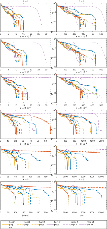
Figure 4.1: Rail at $n=79841$

Figure 4.1 shows the midway convergence behavior for the case $n=79841$ in forms of both time (in seconds) vs. accuracy ($\operatorname{NRes}_{*}$) and the numbers of rows of $\Xi$ vs. accuracy. Note that part of curves stopping decreasing would be cut in order to enlarge the convergent curves.

Table 4.1: Results: Rail

Rail	$r=1$				$r=2,10^{-5}$				$r=2,10^{-4}$				$r=2,10^{-3}$				$r=2,10^{-2}$				$r=5$
shift	ite	dim	time	remark	ite	dim	time	remark	ite	dim	time	remark	ite	dim	time	remark	ite	dim	time	remark	ite	dim	time	remark
$n=1357$				$\,=\,$.1s				$\,=\,$.1s				$\,=\,$.1s				$\,=\,$.1s				$\,=\,$.8s				$\,=\,$.8s
pre	74	444	0.176		74	444	0.215		74	462	0.204		74	767	0.244		74	1462	0.363		74	1888	0.986
hami 1	38	228	0.137		38	228	0.132		38	234	0.108		39	410	0.131		54	1030	0.240		69	1455	0.688
hami 2	39	212	0.111		39	212	0.121		39	218	0.110		58	534	0.185		97	1572	0.402		125	2120	1.051
hami 5	52	282	0.119		52	282	0.147		53	294	0.147		112	878	0.342		160	2279	0.688		227	3328	1.755
hami c 1	36	210	0.119		36	210	0.114		36	205	0.132		40	422	0.161		51	1052	0.312		59	1428	1.048
hami c 2	30	176	0.088		30	176	0.102		28	174	0.096		33	380	0.166		65	1026	0.432		55	1213	0.895
hami c 5	29	174	0.122		29	174	0.132		29	177	0.135		31	354	0.258		300	4906	4.392	4.884e-05	300	5219	6.259	4.858e-05
proj 1	37	220	0.107		37	220	0.119		38	228	0.109		36	414	0.127		57	1222	0.271		65	1742	0.890
proj 2	35	210	0.084		35	210	0.097		35	216	0.097		58	532	0.185		94	1591	0.408		120	2223	1.170
proj 5	68	314	0.152		68	314	0.187		68	323	0.177		112	887	0.342		146	1960	0.551		210	2846	1.581
proj c 1	30	180	0.082		30	180	0.095		31	196	0.100		31	453	0.142		52	1947	0.436		58	3059	1.663
proj c 2	49	294	0.145		49	294	0.161		49	304	0.163		49	1055	0.327		268	10375	2.914		300	16991	10.857	2.786e-03
proj c 5	68	408	0.236		68	408	0.273		68	419	0.272		300	7683	4.904	1.588e-02	300	11885	8.996	1.749e-02	300	17881	21.923	1.771e-02
$n=5177$				$\,=\,$.4s				$\,=\,$.4s				$\,=\,$.8s				$\,=\,$.8s				$\,=\,$1.6s				$\,=\,$3.2s
pre	74	444	0.625		74	444	0.726		74	473	0.788		74	833	0.985		74	1653	1.586		74	2178	4.244
hami 1	43	258	0.393		43	258	0.449		43	267	0.479		46	534	0.578		80	1868	1.825		90	2655	4.700
hami 2	42	240	0.388		42	240	0.461		42	248	0.450		64	710	0.840		111	2568	2.426		137	3738	6.502
hami 5	68	370	0.651		68	370	0.759		67	374	0.724		132	1161	1.552		187	3759	3.654		237	5448	9.384
hami c 1	42	249	0.480		42	249	0.531		37	232	0.481		48	522	0.711		70	1669	1.948		152	2983	5.952
hami c 2	38	228	0.447		38	228	0.505		36	223	0.470		42	529	0.715		300	6933	9.084	1.999e-05	288	4099	9.427
hami c 5	34	191	0.451		34	191	0.564		34	199	0.499		115	1138	2.571		300	6667	15.229	6.051e-05	300	7369	22.933	5.950e-05
proj 1	39	234	0.373		39	234	0.469		39	245	0.437		51	593	0.708		70	1779	1.653		85	2586	4.908
proj 2	45	262	0.445		45	262	0.489		45	273	0.528		62	683	0.830		105	2352	2.205		134	3342	6.202
proj 5	67	334	0.598		67	334	0.721		68	350	0.689		141	1127	1.744		172	2905	2.951		227	3994	7.795
proj c 1	34	204	0.380		34	204	0.418		35	231	0.453		34	555	0.652		58	2466	2.513		62	3876	7.896
proj c 2	55	330	0.623		55	330	0.706		54	352	0.681		58	1067	1.438		300	13979	16.030	9.740e-04	300	21221	46.063	1.319e-02
proj c 5	77	462	1.160		77	462	1.196		145	980	2.600		300	9049	18.157	1.824e-02	300	13645	26.907	1.793e-02	300	21405	77.577	1.850e-02
$n=20209$				$\,=\,$2s				$\,=\,$2s				$\,=\,$2s				$\,=\,$4s				$\,=\,$20s				$\,=\,$80s
pre	74	444	3.514		74	444	3.907		74	482	3.997		74	902	5.060		74	1852	7.739		74	2485	19.612
hami 1	44	264	2.139		44	264	2.291		44	277	2.348		58	702	4.090		97	2519	10.101		114	3829	27.219
hami 2	46	276	2.119		46	276	2.550		46	284	2.543		73	881	5.085		129	3315	13.241		156	5105	36.127
hami 5	72	407	3.349		72	407	3.798		72	412	3.835		159	1438	9.801		248	5532	23.068		272	8304	58.747
hami c 1	59	354	3.009		59	354	3.513		39	247	2.333		52	634	4.139		73	1830	8.720		95	2855	22.777
hami c 2	42	252	2.338		42	252	2.617		43	250	2.672		55	687	4.952		300	8956	46.279	2.514e-04	300	10817	90.851	2.916e-04
hami c 5	40	225	2.697		40	225	2.867		41	239	2.977		143	1410	13.949		300	8494	75.660	1.165e-04	300	10370	133.669	1.211e-04
proj 1	48	277	2.367		48	277	2.486		48	290	2.546		58	757	4.240		74	2214	8.594		90	3388	24.858
proj 2	46	276	2.200		46	276	2.521		46	289	2.477		65	830	4.714		114	3091	12.208		143	4547	33.706
proj 5	69	411	3.356		69	411	3.725		69	412	3.797		143	1345	8.785		197	4121	17.840		260	5929	46.365
proj c 1	38	228	1.958		38	228	2.210		38	269	2.380		38	689	3.741		51	2474	10.286		53	4000	32.607
proj c 2	61	366	3.467		61	366	3.817		60	424	4.042		68	1583	8.919		273	13870	69.869		297	22034	199.092
proj c 5	85	510	5.781		85	510	6.323		300	2413	25.151	1.785e-02	300	10719	103.627	1.820e-02	300	15399	167.329	1.817e-02	300	24667	469.599	1.834e-02
$n=79841$				$\,=\,$10s				$\,=\,$10s				$\,=\,$10s				$\,=\,$20s				$\,=\,$40s				$\,=\,$80s
pre	74	444	14.339		74	444	16.530		74	501	17.080		74	980	24.216		74	2039	35.903		74	2795	94.600
hami 1	45	270	9.069		45	270	10.312		45	290	10.478		66	868	19.661		115	3133	55.269		139	4678	151.880
hami 2	51	306	10.030		51	306	11.613		51	318	11.697		87	1043	25.054		173	4462	82.862		175	6275	199.616
hami 5	77	437	15.031		77	437	17.189		79	452	17.680		179	1774	47.518		300	7165	135.768	1.515e-08	300	10325	326.825	4.601e-09
hami c 1	54	324	11.932		54	324	13.439		49	294	12.185		68	758	21.371		109	2454	55.983		86	2790	100.886
hami c 2	47	266	10.674		47	266	12.066		44	266	11.513		76	897	27.352		300	10168	253.725	4.862e-04	300	12198	470.670	5.338e-04
hami c 5	45	259	12.960		45	259	14.263		45	268	14.415		159	1554	66.590		300	9803	422.460	2.524e-04	300	12080	738.199	2.592e-04
proj 1	53	308	10.427		53	308	11.997		53	330	12.222		63	924	20.076		89	2863	50.626		104	4397	141.570
proj 2	56	328	10.973		56	328	12.625		56	348	12.833		93	1212	27.917		128	3912	69.601		155	5808	186.726
proj 5	73	437	14.380		73	437	16.511		73	459	16.755		140	1521	38.780		213	5242	93.561		273	7793	256.540
proj c 1	41	246	9.071		41	246	10.255		41	299	10.809		42	885	19.401		63	3490	68.597		62	5346	195.384
proj c 2	68	408	15.509		68	408	17.506		68	487	18.854		79	2040	48.893		300	17743	442.668	2.876e-04	300	28129	1198.404	2.690e-03
proj c 5	93	558	27.262		93	558	30.055		300	2419	108.313	1.812e-02	300	12472	571.087	1.827e-02	300	17147	937.535	1.824e-02	300	28759	2664.699	1.836e-02

Example 4.2 (Lung2$-$).

The example is generated in this way: $-A$ is the matrix lung2 in the SuiteSparse Matrix Collection [11] (formerly the University of Florida Sparse Matrix Collection), modelling temperature and water vapor transport in the human lung; $B,C$ are generated by MATLAB function rand. Here $n=109460,\operatorname{nnz}(A)=492564,m=10,l=5$ and $B,C$ are dense matrices.

The heuristic shifts are chosen as $\gamma=3\times 10^{5},3\times 10^{4},\dots,3\times 10^{-2}$ periodically as stated above.

In this example $A$ is nonsymmetric and the eigenvalues of $A$ lie in the left half plane, namely $A$ is stable. Similarly to Example 4.1, the system at $r=1$ is stable, while the systems at $r=2$ and $5$ are not guaranteed to be stable or stabilizable.

For this example we adopt in an additional stopping criterion: the number of rows of $\Xi$ reaches $50000$, for $\Xi$ is a dense matrix and a $50000\times n$ matrix occupies about 40.8GB that is too large.

Moreover, we make another round of test to observe the affect of truncations, with a different truncation criterion: $\|E_{(k)}\|_{*}\leq 10^{-10}$. To cooperate with that, the stopping criteria are changed to: $\operatorname{NRes}_{*}(X_{(k)})<10^{-10}$; or the number of loops reaches $300$; or the difference of $\operatorname{NRes}$ and the accumulated truncation errors in all compressions diminishes under $10^{-10}$.

The results in two rounds are collected in Table 4.2, where the flag “m” indicates that the number of rows of $\Xi$ approaches $50000$, and the flag “t” indicates that the total $\operatorname{NRes}$ does not satisfy the criteria but the one with the accumulated truncation error uncounted does. The midway convergent behavior for the large truncation case is shown in Figure 4.2.

Table 4.2: Results: Lung2$-$

Lung2$-$	$r=1$				$r=2,10^{-8}$				$r=2,10^{-6}$				$r=2,10^{-4}$				$r=2,10^{-2}$				$r=5$
shift	ite	dim	time	remark	ite	dim	time	remark	ite	dim	time	remark	ite	dim	time	remark	ite	dim	time	remark	ite	dim	time	remark
				$\,=\,$28s				$\,=\,$36s				$\,=\,$64s				$\,=\,$160s
pre	300	1388	95.065	1.195e-11	300	3841	151.924	1.218e-11	300	12424	326.361	1.238e-11	300	35157	770.544	1.273e-11	142	49690	1193.109	m  9.659e-08	135	49803	3569.097	m  1.604e-07
hami 1	225	1068	72.118		227	2640	111.937		242	7538	211.564		285	22685	562.064		151	49956	1189.453	m  3.483e-01	136	49733	3616.463	m  6.007e-01
hami 2	221	1029	69.421		238	2864	118.630		253	8231	217.259		300	24173	593.969	6.230e-04	149	49745	1182.042	m  3.622e-01	143	49958	3487.781	m  6.280e-01
hami 5	259	1202	81.357		249	2889	122.105		300	9514	254.030	7.083e-08	300	32476	714.833	7.591e-04	149	49745	1315.983	m  3.622e-01	143	49958	3515.085	m  6.280e-01
hami c 1	209	972	75.662		215	2567	122.405		227	6833	232.828		300	19915	649.161	6.253e-04	154	49816	1736.838	m  3.437e-01	145	49714	4351.744	m  3.628e-01
hami c 2	214	1070	83.045		300	3111	172.548	1.363e-09	300	12383	489.086	5.200e-07	300	37584	1523.890	8.527e-04	164	49972	2988.868	m  4.268e-01	139	49980	5576.575	m  4.306e-01
hami c 5	300	1500	142.640	8.270e-08	300	4326	306.000	4.553e-10	300	18448	1395.591	2.193e-06	300	31149	3209.602	9.156e-04	173	49904	13150.396	m  4.275e-01	145	49714	17241.920	m  4.311e-01
proj 1	205	961	65.037		219	2416	105.445		261	8230	217.629		300	27798	668.425	7.814e-01	207	49880	1296.299	m  7.990e-01	186	49634	3254.690	m  7.998e-01
proj 2	213	1008	67.619		247	2811	119.852		300	9812	255.872	6.815e-10	300	29246	647.732	7.972e-01	248	49838	1177.181	m  7.996e-01	216	49868	3142.694	m  8.000e-01
proj 5	279	1346	92.933		300	3726	151.791	6.997e-01	300	13008	316.733	7.979e-01	300	22186	498.987	7.993e-01	300	42067	1012.625	8.001e-01	223	49946	3231.155	m  8.000e-01
proj c 1	275	1341	96.837		300	3023	156.986	1.038e-01	300	10245	315.674	7.981e-01	300	9751	315.085	8.298e-01	300	19126	543.366	8.509e-01	300	31839	1798.403	8.613e-01
proj c 2	300	1500	110.897	7.907e-01	300	3741	190.756	7.918e-01	300	4352	205.108	8.178e-01	300	7503	287.975	9.355e-01	300	10788	389.053	9.819e-01	300	16904	1025.207	9.819e-01
proj c 5	300	1500	143.600	9.996e-01	300	1500	153.648	9.996e-01	300	2406	183.203	9.996e-01	300	4779	297.800	9.996e-01	300	6260	378.961	9.996e-01	300	10161	882.586	9.996e-01
large truncation 1e-10
pre	244	1000	76.531	t  3.603e-10	244	1000	83.739	t  3.799e-10	244	1063	86.569	t  1.336e-09	244	2424	110.943	t  5.932e-09	244	14490	338.880	t  1.477e-08	244	16744	869.879	t  1.506e-08
hami 1	161	651	52.061	t  4.746e-10	166	667	60.908	t  5.538e-10	182	767	64.277	t  1.195e-09	152	1564	71.166	t  5.306e-09	243	9503	258.963	t  1.404e-08	248	11611	614.994	t  1.586e-08
hami 2	158	636	54.968	t  4.785e-10	156	649	56.980	t  5.383e-10	158	707	57.822	t  1.377e-09	188	1823	85.610	t  5.871e-09	300	9825	262.684	1.607e-08	300	11758	633.241	1.808e-08
hami 5	192	772	65.792	t  4.751e-10	189	787	67.087	t  5.483e-10	193	836	69.512	t  1.159e-09	199	1853	89.338	t  5.601e-09	300	10346	271.767	2.774e-01	300	11897	638.888	1.842e-02
hami c 1	148	615	52.813	t  4.702e-10	160	655	63.621	t  5.708e-10	300	1799	128.069	1.891e-01	167	1686	87.417	t  6.249e-09	300	9303	329.797	2.080e-01	300	11466	701.564	2.143e-01
hami c 2	161	661	63.173	t  4.766e-10	165	669	67.543	t  5.802e-10	182	921	78.344	t  1.056e-09	198	1946	111.595	t  7.888e-09	300	15307	567.969	3.078e-01	300	18077	1163.186	3.070e-01
hami c 5	300	1218	132.194	1.209e-08	300	1237	134.307	3.739e-09	300	1505	151.814	5.314e-07	300	3610	255.586	7.465e-04	300	15833	1130.226	4.236e-01	300	18490	1867.696	4.280e-01
proj 1	179	723	58.178	t  3.842e-10	179	723	65.857	t  4.182e-10	177	728	64.344	t  9.819e-10	186	1513	80.139	t  5.044e-09	279	9464	263.219	t  1.702e-08	285	11940	627.683	t  1.926e-08
proj 2	152	691	53.414	t  3.866e-10	154	709	57.612	t  3.918e-10	154	711	56.334	t  1.096e-09	179	1666	80.215	t  6.465e-09	300	11228	285.698	7.191e-01	300	13812	708.079	7.860e-01
proj 5	230	1075	75.402	t  3.893e-10	230	1075	82.369	t  4.003e-10	235	1086	86.206	t  1.045e-09	300	2431	128.420	8.261e-09	300	14644	359.886	7.993e-01	300	15840	782.248	7.990e-01
proj c 1	166	796	60.837	t  3.824e-10	166	796	68.721	t  4.204e-10	168	806	68.774	t  9.047e-10	181	1579	89.043	t  5.933e-09	300	11521	355.818	7.975e-01	300	13687	771.156	7.982e-01
proj c 2	300	941	111.483	7.759e-01	300	941	116.237	7.778e-01	300	945	114.284	7.899e-01	300	2450	155.020	7.844e-01	300	3513	177.289	8.095e-01	300	3935	279.611	8.116e-01
proj c 5	300	1500	141.727	9.996e-01	300	1500	150.211	9.996e-01	300	1500	153.267	9.996e-01	300	1500	153.331	9.996e-01	300	1802	163.526	9.996e-01	300	1802	224.638	9.996e-01

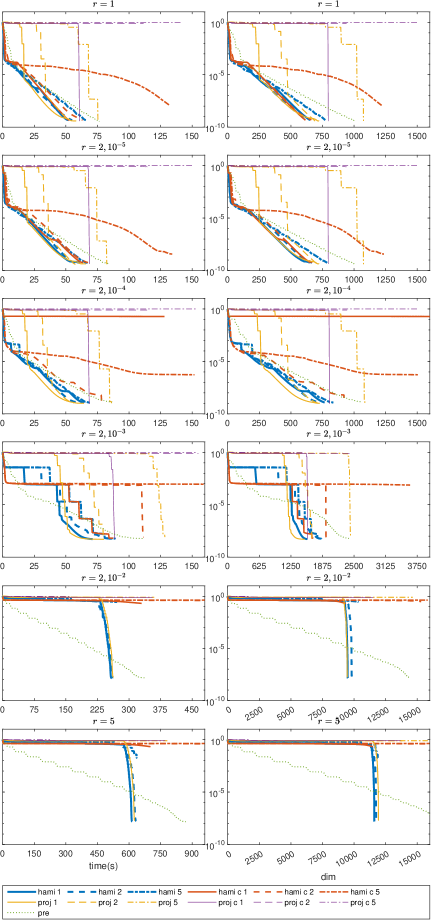
Figure 4.2: Lung2-: large truncation case

Observing the tables and the figures, we may see some features.

Shift strategy

In each shift strategy with different prescribed $s$, usually $s=1$ is the best choice because it takes the least loops, generates the smallest $\Xi$, and consumes the least time with only a few exception. Especially in the cases that the stochastic part is large ($r=5$), there is no exception. The reason that a projection on a large-dimensional subspace are not able to reduce even the number of loops is that the shifts are obtained by computing the terms on the corresponding CARE rather than the SCARE, which would weaken the approximation for a large-dimensional subspace.

For the method that the shifts are not frequent to be computed, including “hami *” and “proj *”, the cost for calculating the shifts is relatively tiny, while for the method that the shifts are computed in each loop, including “hami c *” and “proj c *”, the cost for calculating the shifts cannot be ignored, and even dominate at the large stochastic part cases.

Except the cost of the shifts, for the small stochastic part cases, the main cost is calculating $C_{\gamma}$; for the large stochastic part cases, the main cost is the compression. This coincides with the analysis in Section 3.3. The phenomenon that the cost on the so-called “others” is not small is due to the deep copy of data in the memory, which is unpredictable. This disadvantage would be overcome in the program by the C language.

The shift strategy “hami 1” usually generates the best effort or at least it is one of the best several strategies, which does not exactly coincide with the RADI method for CAREs (that enjoys “hami c 1”) maybe also because the shifts are obtained by computing the terms on the corresponding CARE rather than the SCARE.

Compression/Truncation

The result of truncation, namely $l_{\operatorname{tr}}$, will conclusively determine the running time. Hence a loose truncation criterion will significantly accelerate the process, but it would decrease the accuracy. But for some problem not good enough, it is worthwhile to use a loose one, for its Return on Investment is relatively large, as is shown in Table 4.2 and Figure 4.2.

Compared the results at $l=5$ in Table 4.2 and those generated by RADI at $l=10$ in [1, Table 3] on CARE ($r=1$), we may see the compression would slow down the convergence. This phenomenon is reasonable, for part of useful information are discarded in the compression, and it is a trade-off between convergence and storage. We have to compress for the true SCARE case ($r>1$) to avoid the exponential increase of the size of $\Xi$.

Comparison

In the experiments we have not tried comparing our ISC method with some existing methods. Here we simply explain the reason.

• The comparison theorem based method [15] and LMI’s method [28] are not valid for large-scale problems.

• The homotopy method [32], and the Newton-type methods, including the basic variant [9, 10], the modified variant [17, 23] and the GLE-driver variant [14], all face an inconspicuous but very time-consuming point: validating the stopping criteria. Without any low-rank expression of the residual $\mathscr{C}(\widetilde{X})$, one has to calculate it out explicitly and estimate its norm, which is a task over $n\times n$ matrices. To the opposite, equipped with its low-rank expression 2.7 and the discussion in Section 3.1, it is reduced to a task over $rl_{\operatorname{tr}}\times rl_{\operatorname{tr}}$ matrices.

• Moreover, for the Newton-type methods, a fatal problem is how to find a stabilizing initial approximation. [14] argued three times that the initial stabilization for the Newton’s method is a difficult open problem, and its authors did not provide their way to it in the numerical tests. To the opposite, our ISC method does not need any special initialization, which completely avoids to be trapped.

• In detail, the GLE-driver Newton method [14] is only tested on an example with $r=2,\operatorname{nnz}(A_{1})=n-1,\operatorname{nnz}(B_{1})=2$; the homotopy method [32] is only tested on the example Rail with $r=2,\operatorname{nnz}(A_{1})\approx 0.01\operatorname{nnz}(A),\operatorname{nnz}(B_{1})\approx 0.1\operatorname{nnz}(B)$. In comparison, we test Rail with as large as $r=5,\operatorname{nnz}(A_{i})=\operatorname{nnz}(A),\operatorname{nnz}(B_{i})=\operatorname{nnz}(B)$.

5 Conclusion

We have presented our ISC method for computing the unique positive semi-definite stabilizing solution for large-scale stochastic continuous-time algebraic Riccati equations with sparse and low-rank structure. This very efficient method benefits from the algebraic structure of the equations and the RADI method for solving classical continuous-time algebraic Riccati equations. As an evidence, this promising method are able to solve the standard benchmark problem Rail involving four stochastic processes with the same sparsity at $n=79841,r=5,\operatorname{nnz}=553321\times 5$ in 100 seconds with MATLAB on an ordinary PC without any prior information.

Like RADI, its performance highly relies on the strategy of choosing the shifts, among which we suggests using the residual Hamiltonian shift in each loop. Due to lack of results on eigenvalue problem in left semi-tensor product, we have to use real part of a chosen eigenvalue of the projected classical Hamiltonian matrix. We believe that it is very worthwhile to deal with the eigenvalue problem in left semi-tensor product not only for its own significance, but also for its role in shifts to accelerate the method proposed in the paper.

Appendix A Additional Results

Lemma A.1.

Write

$$\widetilde{C}=\sqrt{2\gamma}CA_{\gamma}^{-1}\in\mathbb{R}^{p\times n},\quad\widetilde{B}=\widetilde{\Pi}\begin{bmatrix}\sqrt{2\gamma}A_{\gamma}^{-1}B\\ \widehat{A}A_{\gamma}^{-1}B-\widehat{B}\end{bmatrix}\in\mathbb{R}^{rn\times m},\quad\widetilde{A}=\widetilde{\Pi}\begin{bmatrix}I+2\gamma A_{\gamma}^{-1}\\ \sqrt{2\gamma}\widehat{A}A_{\gamma}^{-1}\end{bmatrix}\in\mathbb{R}^{rn\times n}.$$ (A.1)

Then the sequence $\{X_{t}\}$ generated by the fixed point iteration 2.3 are of the non-iterative equivalent form:

$$X_{t}=V_{t}^{\operatorname{T}}(I+T_{t}T_{t}^{\operatorname{T}})^{-1}V_{t},$$ (A.2)

where

$$V_{t}=\begin{bmatrix}\widetilde{C}\\ \widetilde{C}\ltimes\widetilde{A}\\ \widetilde{C}\ltimes\widetilde{A}^{\ltimes 2}\\ \vdots\\ \widetilde{C}\ltimes\widetilde{A}^{\ltimes(t-1)}\end{bmatrix}_{\frac{r^{t}-1}{r-1}p\times n},\quad T_{t}=\operatorname{\mathcal{L}}_{r,p,m}\left(\begin{bmatrix}Y_{\gamma}\\ \widetilde{C}\ltimes\widetilde{B}\\ \widetilde{C}\ltimes\widetilde{A}\ltimes\widetilde{B}\\ \vdots\\ \widetilde{C}\ltimes\widetilde{A}^{\ltimes(t-2)}\ltimes\widetilde{B}\end{bmatrix}\right)_{\frac{r^{t}-1}{r-1}p\times\frac{r^{t}-1}{r-1}m},\quad T_{1}=Y_{\gamma}.$$ (A.3)

Proof.

First 2.2 can be rewritten as

$$E_{\gamma}=\widetilde{A}-\widetilde{B}Y_{\gamma}^{\operatorname{T}}(I+Y_{\gamma}Y_{\gamma}^{\operatorname{T}})^{-1}\widetilde{C},\quad H_{\gamma}=\widetilde{C}^{T}(I_{l}+Y_{\gamma}Y_{\gamma}^{T})^{-1}\widetilde{C},\quad G_{\gamma}=\widetilde{B}(I+Y_{\gamma}^{\operatorname{T}}Y_{\gamma})^{-1}\widetilde{B}^{\operatorname{T}}.$$ (A.4)

Then A.2 is correct for $t=1$. Assuming A.2 is correct for $t$, we will immediately prove it is also correct for $t+1$. Plugging A.4 in 2.3, we have

$$X_{t+1} =H_{\gamma}+E_{\gamma}^{T}\ltimes V_{t}^{\operatorname{T}}(I+T_{t}T_{t}^{\operatorname{T}})^{-1}V_{t}\ltimes\left(I_{rn}+G_{\gamma}\ltimes V_{t}^{\operatorname{T}}(I+T_{t}T_{t}^{\operatorname{T}})^{-1}V_{t}\right)^{-1}\ltimes E_{\gamma}$$

$$\stackrel{{\scriptstyle\makebox[0.0pt][c]{\scriptsize\lx@cref{creftype~refnum}{eq:easy}}}}{{=}}\;\widetilde{C}^{\operatorname{T}}(I+Y_{\gamma}Y_{\gamma}^{\operatorname{T}})^{-1}\widetilde{C}+E_{\gamma}^{\operatorname{T}}\ltimes V_{t}^{\operatorname{T}}\ltimes\left(I_{rn}+(T_{t}T_{t}^{\operatorname{T}})\otimes I_{r}+V_{t}\ltimes G_{\gamma}\ltimes V_{t}^{\operatorname{T}}\right)^{-1}\ltimes V_{t}\ltimes E_{\gamma}$$

$$=\begin{bmatrix}\widetilde{C}\\ V_{t}\ltimes E_{\gamma}\end{bmatrix}^{\operatorname{T}}\begin{bmatrix}I+Y_{\gamma}Y_{\gamma}^{\operatorname{T}}&\\ &I+(T_{t}T_{t}^{\operatorname{T}})\otimes I_{r}+V_{t}\ltimes\widetilde{B}(I+Y_{\gamma}^{\operatorname{T}}Y_{\gamma})^{-1}\widetilde{B}^{\operatorname{T}}\ltimes V_{t}^{\operatorname{T}}\end{bmatrix}^{-1}\begin{bmatrix}\widetilde{C}\\ V_{t}\ltimes E_{\gamma}\end{bmatrix}$$

$$=(*)^{\operatorname{T}}\begin{bmatrix}I+Y_{\gamma}Y_{\gamma}^{\operatorname{T}}&\\ &I+(T_{t}T_{t}^{\operatorname{T}})\otimes I_{r}+V_{t}\ltimes G_{\gamma}\ltimes V_{t}^{T}\end{bmatrix}^{-1}\underline{\begin{bmatrix}I&\\ -V_{t}\ltimes\widetilde{B}Y_{\gamma}^{\operatorname{T}}(I+Y_{\gamma}Y_{\gamma}^{\operatorname{T}})^{-1}&I\end{bmatrix}\begin{bmatrix}\widetilde{C}\\ V_{t}\ltimes\widetilde{A}\end{bmatrix}}$$

$$\qquad\!\!\underbracket{\hskip 341.43306pt}$$

$$\stackrel{{\scriptstyle\makebox[0.0pt][c]{\scriptsize\lx@cref{creftype~refnum}{eq:smwf}}}}{{=}}\;\begin{bmatrix}\widetilde{C}\\ V_{t}\ltimes\widetilde{A}\end{bmatrix}^{\operatorname{T}}\begin{bmatrix}I+Y_{\gamma}Y_{\gamma}^{\operatorname{T}}&Y_{\gamma}\widetilde{B}^{\operatorname{T}}\ltimes V_{t}^{\operatorname{T}}\\ V_{t}\ltimes\widetilde{B}Y_{\gamma}^{\operatorname{T}}&I+(T_{t}T_{t}^{\operatorname{T}})\otimes I_{r}+V_{t}\ltimes\widetilde{B}\widetilde{B}^{\operatorname{T}}\ltimes V_{t}^{\operatorname{T}}\end{bmatrix}^{-1}\begin{bmatrix}\widetilde{C}\\ V_{t}\ltimes\widetilde{A}\end{bmatrix}$$

$$=\begin{bmatrix}\widetilde{C}\\ V_{t}\ltimes\widetilde{A}\end{bmatrix}^{\operatorname{T}}\left(I+\begin{bmatrix}Y_{\gamma}&0\\ V_{t}\ltimes\widetilde{B}&T_{t}\otimes I_{r}\end{bmatrix}\begin{bmatrix}Y_{\gamma}&0\\ V_{t}\ltimes\widetilde{B}&T_{t}\otimes I_{r}\end{bmatrix}^{\operatorname{T}}\right)^{-1}\begin{bmatrix}\widetilde{C}\\ V_{t}\ltimes\widetilde{A}\end{bmatrix}$$

$$=V_{t+1}^{\operatorname{T}}(I+T_{t+1}T_{t+1}^{\operatorname{T}})^{-1}V_{t+1}.\qed$$

References

- [1] P. Benner, Z. Bujanović, P. Kürschner, and J. Saak. RADI: a low-rank ADI-type algorithm for large-scale algebraic Riccati equations. Numer. Math., 138:301–330, 2018.
- [2] P. Benner, J.-R. Li, and T. Penzl. Numerical solution of large Lyapunov equations, Riccati equations, and linear-quadratic control problems. Numer. Lin. Alg. Appl., pages 755–777, 2008.
- [3] Peter Benner, Zvonimir Bujanović, Patrick Kürschner, and Jens Saak. A numerical comparison of different solvers for large-scale, continuous-time algebraic Riccati equations and LQR problems. SIAM J. Sci. Comput., 42(2):A957–A996, 2020.
- [4] D. A. Bini, B. Iannazzo, and B. Meini. Numerical Solution of Algebraic Riccati Equations, volume 9 of Fundamentals of Algorithms. SIAM Publications, Philadelphia, 2012.
- [5] Daizhan Cheng. Semi-tensor product of matrices and its applications to Morgan’s problem. Sci. China, Ser. F: Info. Sci., 44(3):195–212, 2001.
- [6] Daizhan Cheng. From Dimension-Free Matrix Theory to Cross-Dimensional Dynamic Systems. Mathematics in Science and Engineering. Academic Press, 2019.
- [7] Daizhan Cheng and Hongsheng Qi. Controllability and observability of Boolean control networks. Automatica, 45(7):1659–1667, 2009.
- [8] Eric King-wah Chu, Tiexiang Li, Wen-Wei Lin, and Chang-Yi Weng. A modified newton’s method for rational riccati equations arising in stochastic control. In 2011 International Conference on Communications, Computing and Control Applications (CCCA), pages 1–6, 2011.
- [9] T. Damm and D. Hinrichsen. Newton’s method for a rational matrix equation occurring in stochastic control. Linear Algebra Appl., 332-334:81–109, 2001.
- [10] Tobias Damm. Rational Matrix Equations in Stochastic Control. Springer-Verlag, Berlin/Heidelberg, Germany, 2004.
- [11] Timothy A. Davis and Yifan Hu. The university of Florida sparse matrix collection. ACM Trans. Math. Software, 38(1):Article 1, 2011. 25 pages.
- [12] Vasile Dragan, Toader Morozan, and Adrian-Mihail Stoica. Mathematical Methods in Robust Control of Discrete-Time Linear Stochastic Systems. Springer-Verlag, New York, NY, USA, 2010.
- [13] Vasile Dragan, Toader Morozan, and Adrian-Mihail Stoica. Mathematical Methods in Robust Control of Linear Stochastic Systems. Springer-Verlag, New York, NY, USA, 2nd edition, 2013.
- [14] Hung-Yuan Fan, Peter Chang-Yi Weng, and Eric King wah Chu. Smith method for generalized Lyapunov/Stein and rational Riccati equations in stochastic control. Numer. Alg., 71:245–272, 2016.
- [15] G. Freiling and A. Hochhaus. Properties of the solutions of ration matrix difference equations. Computers Math. Appl., 45:1137–1154, 2003.
- [16] G. Freiling and A. Hochhaus. On a class of rational matrix differential equations arising in stochastic control. Linear Algebra Appl., 379:43–68, 2004.
- [17] Chun-Hua Guo. Iterative solution of a matrix Riccati equation arising in stochastic control. Oper. Theory: Adv. Appl., 130:209–221, 2001.
- [18] Zhen-Chen Guo and Xin Liang. The intrinsic Toeplitz structure and its applications in algebraic Riccati equations. Numer. Alg., 93:227–267, 2023.
- [19] Zhen-Chen Guo and Xin Liang. Stochastic algebraic Riccati equations are almost as easy as deterministic ones theoretically. SIAM J. Matrix Anal. Appl., 44(4):1749–1770, 2023.
- [20] T.-M. Huang, R.-C. Li, and W.-W. Lin. Structure-Preserving Doubling Algorithms for Nonlinear Matrix Equations, volume 14 of Fundamentals of Algorithms. SIAM, Philadelphia, 2018.
- [21] Hideaki Iiduka and Isao Yamada. Computational method for solving a stochastic linear-quadratic control problem given an unsolvable stochastic algebraic Riccati equation. SIAM J. Control Optim., 50(4):2173–2192, 2012.
- [22] Vlad Ionescu, Cristian Oară, and Martin Weiss. Generalized Riccati Theory and Robust Control: A Popov Function Approach. John Wiley & Sons, Chichester, UK, 1999.
- [23] Ivan Ganchev Ivanov. Iterations for solving a rational Riccati equations arising in stochastic control. Computers Math. Appl., 53:977–988, 2007.
- [24] Ivan Ganchev Ivanov. Properties of Stein (Lyapunov) iterations for solving a general Riccati equation. Nonlinear Anal. Theory Methods Appl., 67:1155–1166, 2007.
- [25] P. Lancaster and L. Rodman. Algebraic Riccati Equations. The clarendon Press, Oxford Sciece Publications, New York, 1995.
- [26] V. L. Mehrmann. The autonomous linear quadratic control problems. In Lecture Notes in Control and Information Sciences, volume 163. Springer-Verlag, Berlin, 1991.
- [27] Oberwolfach Benchmark Collection. Steel profile. hosted at MORwiki – Model Order Reduction Wiki, 2005.
- [28] Mustapha Ait Rami and Xun Yu Zhou. Linear matrix inequalities, Riccati equations, and indefinite stochastic linear quadratic controls. IEEE Trans. Automat. Control, 45(6):1131–1143, 2000.
- [29] J. Saak, M. Köhler, and P. Benner. M-M.E.S.S.-2.1 – the matrix equations sparse solvers library, April 2021. see also: https://www.mpi-magdeburg.mpg.de/projects/mess.
- [30] Nobuya Takahashi, Michio Kono, Tatsuo Suzuki, and Osamu Sato. A numerical solution of the stochastic discrete algebraic Riccati equation. J. Archaeological Sci., 13:451–454, 2009.
- [31] Ancheng Xue and Shengwei Mei. A new transient stability margin based on dynamical security region and its applications. Sci. China, Ser. E: Tech. Sci., 51(6):750–760, 2008.
- [32] Liping Zhang, Hung-Yuan Fan, Eric King wah Chu, and Yimin Wei. Homotopy for rational Riccati equations arising in stochastic optimal control. SIAM J. Sci. Comput., 37(1):B103–B125, 2015.