Galled Tree-Child Networks
Abstract
We propose the class of galled tree-child networks which is obtained as intersection of the classes of galled networks and tree-child networks. For the latter two classes, (asymptotic) counting results and stochastic results have been proved with very different methods. We show that a counting result for the class of galled tree-child networks follows with similar tools as used for galled networks, however, the result has a similar pattern as the one for tree-child networks. In addition, we also consider the (suitably scaled) numbers of reticulation nodes of random galled tree-child networks and show that they are asymptotically normal distributed. This is in contrast to the limit laws of the corresponding quantities for galled networks and tree-child networks which have been both shown to be discrete.
Dedicated to Hsien-Kuei Hwang on the occasion of his 60th birthday
1 Introduction
Phylogenetic networks are used to visualize, model, and analyze the ancestor relationship of taxa in reticulate evolution. To make them more relevant for biological applications as well as devise algorithms for them, many subclasses of the class of phylogenetic networks have been proposed; see the comprehensive survey [13]. A lot of recent research work was concerned with fundamental questions such as counting them and understanding the shape of a network drawn uniformly at random from a given class; see, e.g., [2, 3, 4, 7, 8, 10, 11, 9, 12, 14, 15]. Despite of this, even counting results are still missing for most of the major classes of phylogenetic networks. Two notable exceptions are tree-child networks and galled networks for which such results have been proved in [10, 11]. In this work, we consider the intersection of these two network classes. We start with some basic definitions and then explain why we find this class interesting.
First, a phylogenetic network is defined as follows.
Definition 1.1 (Phylogenetic Network).
A (rooted) phylogenetic network of size is a rooted, simple, directed, acyclic graph whose nodes fall into the following three (disjoint) categories:
-
(a)
A unique root which has indegree and outdegree ;
-
(b)
Leaves which have indegree and outdegree and are bijectively labeled with labels from the set ;
-
(c)
Internal nodes which have indegree and outdegree at least and total degree at least .
Moreover, a phylogenetic network is called binary if (c) is replaced by
-
(c’)
Internal nodes which have either indegree and outdegree (tree nodes) or indegree and outdegree (reticulation nodes).
Remark 1.2.
-
(i)
Phylogenetic networks with all internal nodes having indegree equal to are called phylogentic trees.
-
(ii)
If not explicitly mentioned, phylogenetic networks will always be binary in the sequel.
We next define galled networks and tree-child networks which are two of the major classes of phylogenetic networks. For the definition, we need the notion of a tree cycle which is a pair of edge-disjoint paths in a phylogenetic network that start at a common tree node and end at a common reticulation node with all other nodes being tree nodes.
Definition 1.3.
-
(a)
A phylogenetic network is called a tree-child network if every non-leaf node has at least one child which is either a reticulation node or a leaf.
-
(b)
A phylogenetic network is called a galled network if every reticulation node is in a (necessarily unique) tree cycle.
Remark 1.4.
Note that neither the class of tree-child networks is contained in the class of galled networks nor vice versa.
Let and denote the number of tree-child networks and galled networks of size with reticulation nodes, respectively. It is not hard to see that for tree-child networks and for galled networks where both bounds are sharp. Thus, the total numbers are given by:
| (1) |
The asymptotic growth of both of these sequences is known. First, in [10], it was proved that for the number of tree-child networks, as ,
| (2) |
where is the largest root of the Airy function of the first kind. The surprise here was the presence of a stretched exponential in the asymptotic growth term. On the other hand, no stretched exponential is contained in the asymptotics of the number of galled networks. More precisely, it was proved in [11] that
| (3) |
The tools used to establish (2) and (3) were very different: for (2), a bijection to a class of words was proved and a recurrence for these word was found which could be (asymptotically) analyzed with the approach from [6]; for (3), the component graph method introduced in [12] together with the Laplace method and a result from [1] was used.
Another difference was the location in (1) of the terms which dominate the two sums. For tree-child networks, the main contribution comes from networks with close to (the maximal-reticulated networks), whereas for galled networks, the main contributions comes from networks with . In fact, the limit law of the number of reticulation nodes, say , was derived in [5, 11] for both network classes if a network of size is sampled uniformly at random. More precisely, for tree-child networks, it was shown in [5] that, as ,
where denotes convergence in distribution and is a Poisson law with parameter . A similar discrete limit law was proved in [11] for galled networks, however, the limit law is not Poisson but a mixture of Poisson laws; see Theorem 2 in [11] for details.
Due to the above results and differences, one wonders how the intersection of the class of tree-child networks and galled networks behaves?
Definition 1.5 (Galled Tree-Child Network).
A galled tree-child network is a network which is both a galled network and a tree-child network.
Let denote the number of galled tree-child networks of size with reticulation nodes. We will show below that . (See Lemma 3.1 in Section 3.) Set:
Then, this sequence has the following first-order asymptotics.
Theorem 1.6.
For the number of galled tree-child networks, we have, as ,
Remark 1.7.
We next consider the number of reticulation nodes of a random galled tree-child network which is a galled tree-child network of size that is sampled uniformly at random from the set of all galled tree-child networks of size . In contrast to tree-child networks and galled networks, the limit law of (suitably scaled) is continuous.
Theorem 1.8.
The number of reticulation nodes of a random galled tree-child networks satisfies, as ,
where denotes the standard normal distribution. Moreover,
The above results show that galled tree-child networks behave quite different from both tree-child networks and galled networks. That is one reason why we find them interesting.
Another reason stems from a recent result which was proved in [4]. In the latter paper, the asymptotics of for fixed was derived. Let denote the number of phylogenetic networks of size and reticulation nodes. (Note that this number is finite, whereas it becomes infinite when summing over .) Then, one of the main results from [4] implies that for fixed , as ,
| (4) |
(The first two asymptotic equivalences were proved in [9, 14].) That and have the same first-order asymptotics for fixed was a surprise since the classes of tree-child networks and galled networks are quite different, e.g., neither contains the other; see Remark 1.4. However, the above result can be explained via the class of galled tree-child networks as will be seen in Section 3 below.
We conclude the introduction with a short sketch of the paper. The proofs of Theorem 1.6 and Theorem 1.8 follow with a similar approach as used for galled networks in [10]. This approach is based on the component graph method from [12] which we will recall in the next section. Then, in Section 3, we will consider for small and large values of . Finally, Section 4 will contain the proofs of our main results (Theorem 1.6 and Theorem 1.8). We will conclude the paper with some final remarks in Section 5.
2 The Component Graph Method
The component graph method for galled networks was introduced in [12] and used in [4, 11] to prove asymptotic results. It is explained in detail in all these papers. However, to make the current paper self-contained, we will briefly recall it.
Let be a galled network. Then, by removing all the edges leading to reticulation vertices (these are the so-called reticulation edges), we obtain a forest whose trees are called the tree-components of .
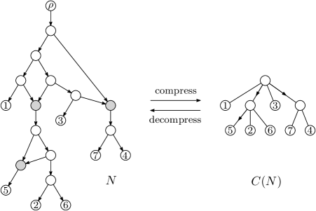
The component graph of , denoted by , is now a rooted, directed, acyclic graph which has a vertex for every tree-component. Moreover, the vertices are connected in the same way as the tree-components have been connected by the reticulation edges. Finally, we attach the leaves in the tree-components to the corresponding vertices in unless a vertex of is a terminal vertex and its corresponding tree-component has exactly one leaf, in which case we use the label of that leaf to label . Note that every non-root vertex in has indegree and that may contain double edges. We will replace such a double edge by a single edge and indicate that it was a double edge by placing an arrow on it; see Figure 1 for a galled network together with its component graph. Also, denote by the component graph of with all arrows on edges removed. Then, the authors of [12] made the following important observation.
Proposition 2.1 ([12]).
is a galled network if and only if is a (not necessarily binary) phylogenetic tree.
The component graph can be seen as a compression of . Thus, in order to generate all galled networks of size , one only needs to list all component graphs (i.e., phylogenetic trees) with labeled leaves and decompress them.
We will next explain the decompression procedure. For this, we need the notion of one-component networks.
Definition 2.2 (One-component Network).
A phylogenetic network is called a one-component network if every reticulation node has a leaf as its child.
Now, let be given. We do a breadth-first traversal of and replace every vertex by a one-component galled network whose leaves below reticulation vertices are labeled with the first labels, where is the number of outgoing edges of in that have an arrow on them, and whose size is equal to the outdegree of . Then, attach the subtrees of which are connected to by edges with arrows on them to the leaves of with labels , where the subtree with the smallest label is attached to , the subtree with the second largest label is attached to , etc. Moreover, relabel the remaining leaves of by the remaining subtrees of (which are all of size , i.e., they are leaves) in an order-consistent way. By using all possible one-component galled networks in every step, this gives all possible galled networks with as component graph. Moreover, if we start from , then we first have to place arrows on all edges whose heads are internal nodes of and for all remaining edges, we can freely decide if we want to place an arrow on them or not. Overall, this gives the following result which was one of the main results of [12].
Proposition 2.3 ([12]).
We have,
where the first sum runs over all (not necessarily binary) phylogenetic trees of size , the product runs over all internal nodes of , is the outdegree of , is the number of children of which are leaves, and denotes the number of one-component galled networks of size with reticulation vertices, where the leaves below the reticulation vertices are labeled with labels from the set .
For galled tree-child networks, it is now clear that the same formula holds with the only difference that has to be replaced by the corresponding number of one-component galled tree-child networks. However, this number is the same as the number of one-component tree-child networks.
Lemma 2.4.
Every one-component tree-child network is a one-component galled tree-child network.
Proof.
Let be a reticulation vertex and consider a pair of edge-disjoint paths from a common tree vertex to . (Note that such a pair trivially exists.) Then, no internal vertex can be a reticulation vertex because such a reticulation vertex would not be followed by a leaf. Thus, is in a tree cycle which shows that the network is indeed galled.
Denote by the number of one-component tree-child networks of size and reticulation vertices, where the labels of the leaves below the reticulation vertices are . Then, we have the following analogous result to Proposition 2.3.
Proposition 2.5.
Remark 2.6.
Using this result, one can obtain the following table for small values of :
| 1 | 1 |
|---|---|
| 2 | 3 |
| 3 | 48 |
| 4 | 1,611 |
| 5 | 87,660 |
| 6 | 6,891,615 |
| 7 | 734,112,540 |
| 8 | 101,717,195,895 |
| 9 | 17,813,516,259,420 |
| 10 | 3,857,230,509,496,875 |
We will deduce all our results from (5). In addition, we will make use of the following results for which were proved in [3] and [10]. To state them, denote by the number of one-component tree-child networks of size with reticulation vertices and by the (total) number of one-component tree-child networks of size . Then,
| (6) |
and
(Note that the tree-child property implies the and this bound is sharp.)
The second result above is a local limit theorem for the (random) number of reticulation vertices of a one-component tree-child network of size which is picked uniformly at random from all one-component tree-child networks of size . It implies the following (asymptotic) counting result for .
Corollary 2.8 ([10]).
As ,
3 Networks with Few and Many Reticulation Nodes
In this section, we consider for small and large . We start with large .
As mentioned in the last section (see the sentence before Proposition 2.7), for tree-child networks, we have that and this bound is sharp. Clearly, this implies that also for galled tree-child networks. Again this bound is sharp.
Lemma 3.1.
The number of reticulation vertices of a galled tree-child network of size is at most where this bound is sharp.
Proof.
Let be a galled tree-child network of size . Consider the component graph of which is a phylogenetic tree of size (see Lemma 2.1). The maximal number of reticulation vertices of is achieved by placing the maximal number of arrows at all outgoing edges of internal vertices of . Note that this the degree of , say , minus , because placing arrows on all outgoing edges is not possible since . Thus, the maximal number of reticulation vertices equals
| (7) |
where the sums run over all internal vertices of . By the handshake lemma,
which, by plugging into (7), gives the claimed result.
The proof of the last lemma also reveals the structure of maximal reticulated galled tree-child networks of size : They are obtained by decompressing component graphs that are phylogenetic trees of size with at least one leaf attached to every internal vertex by placing arrows on all outgoing edges of except the one leading to . This can be translated into generating functions. Set:
where the last line follows from (6) and Proposition 2.7-(i). Then, we have the following result.
Lemma 3.2.
We have,
| (8) |
Proof.
According to the explanation in the paragraph preceding the lemma, a maximal reticulated galled tree-child network is either a leaf or obtained from a maximal reticulated one-component tree-child network with the leafs below the reticulation vertices replaced by maximal reticulation galled tree-child networks. This translates into
where the inside the sum counts the leaf which is not below the reticulation vertex and the factor discards the order of the maximal reticulated galled tree-child networks (counted by ) which are attached to the children below the reticulation vertices. The claimed result follows from this.
Note that (8) is of Lagrangian type. Thus, we can obtain the asymptotics of by applying Lagrange’s inversion formula and the following result from [1].
Theorem 3.3 ([1]).
Let be a formal power series with and . Then, for and real numbers,
Theorem 3.4.
The number of maximal reticulated galled tree-child networks satisfies, as ,
Remark 3.5.
Proof.
We next consider with small, i.e., the other extreme case of the number of reticulation vertices. Here, we have the following result which explains why the asymptotic expansions of and in (4) are the same.
Theorem 3.6.
For fixed , as ,
| (10) |
The proof of this result uses ideas from [9].
Proof.
First consider galled tree-child networks of size which are obtained by decompressing phylogenetic trees of size which have all arrows on the edges from the root, i.e., the root has at least one leaf and all other children are either internal nodes or leaves (with at most internal nodes) and all internal nodes have just leaves as children. By Proposition 8 in [9], the number of these galled tree-child network has the same asymptotics as the one on the right-hand side of (10). Moreover, these networks also dominate the asymptotics in the case of tree-child networks. Thus, the remaining galled tree-child networks are asymptotically negligible as their number is bounded above by the number of remaining tree-child networks.
4 Proof of the Main Results
For the proof of Theorem 1.6, we closely follow the method of proof of (3) from [11]. The main idea is to use (5) to find asymptotic matching upper and lower bounds for .
First, for an upper bound, we pick a phylogenetic tree of size (which is considered to be a component graph of a galled tree-child network of size ) and decompress it by picking for internal vertices of any one-component tree-child network of size (where the notation is as in Proposition 2.3). Since, as explained in Section 2, actually only certain one-component tree-child networks are permissible, this modified decompression procedure overcounts the number of galled tree-child networks of size . More precisely, we consider
where the first sum runs over all phylogenetic trees of size and the product runs over internal vertices of . Then, we have . Next, set
Then, the definition of implies the following result.
Lemma 4.1.
We have,
Proof.
The networks counted by are either a leaf or a one-component tree-child network with leaves which are replaced by an unordered sequence of networks of the same type. This gives
from which the claimed result follows.
Now, we can proceed as in the proof of Theorem 3.4 to obtain the following asymptotic result for .
Proposition 4.2.
As ,
Next, we need a matching lower bound. Therefore, we consider (5) with the first sum restricted to phylogenetic trees of the shape (where we have removed the leaf labels):
We denote the resulting term by . The decompression procedure from Section 2, then gives the following result.
Lemma 4.3.
We have,
| (11) |
Proof.
From this result, we can deduce (matching) first-order asymptotics for which then together with the asymptotics of the upper bound (Proposition 4.2) concludes the proof of Theorem 1.6.
Proposition 4.4.
As ,
Sketch of the proof.
From Stirling’s formula (similar to the proof of Proposition 2.7-(ii)),
where and this holds uniformly for small and (which both may depend on ). Using the Laplace method then gives,
uniformly for small (which again may depend on ). Finally, by plugging the last relation into (11),
which gives the claimed result.
Finally, by refining the above method (see Section 6 of [11] where the same was done for galled networks), we obtain the following result which implies our second main result (Theorem 1.8).
Theorem 4.5.
Let be the number of reticulation vertices of a random galled tree-child network of size which are not followed by a leaf and be the total number of reticulation vertices. Then, as ,
where and are independent with and .
5 Conclusion
In this paper, we introduced the class of galled tree-child network which is obtained as intersection of the classes of galled networks and tree-child networks. Our reason for doing so was two-fold: (i) Different tools have been used to prove results for galled networks and tree-child networks ([10, 11]); consequently, we were curious about which tools apply to the combination of these classes? (ii) It was recently proved that the number of galled networks and tree-child networks have the same first-order asymptotics when the number of reticulation vertices is fixed ([4, 9]). Why is that the case?
As for (i), we showed that an asymptotic counting result for galled tree-child networks (Theorem 1.6) can be obtained with the methods for galled networks, however, the result contains a stretched exponential as does the asymptotic result for tree-child networks. In addition, we showed that the number of reticulation vertices for a random galled tree-child networks is asymptotically normal (Theorem 1.8), whereas the limit laws of the same quantities for galled networks and tree-child networks were discrete. As for (ii), we showed that the number of galled tree-child networks also satisfies the same first order asymptotics when the number of reticulation vertices is fixed. This explains the previous results from [4, 9].
Acknowledgments.
The authors acknowledge partial supported by NTCS, Taiwan under the grants NSTC-111-2115-M-004-002-MY2 (YSC, MF) and NSTC-110-2115-M-017-003-MY3 (GRY).
References
- [1] E. A. Bender and L. B. Richmond (1984). An asymptotic expansion for the coefficients of some power series. II. Lagrange inversion, Discrete Math., 50:2-3, 135–141.
- [2] M. Bouvel, P. Gambette, M. Mansouri (2020). Counting phylogenetic networks of level and level , J. Math. Biol., 81:6-7, 1357–1395.
- [3] G. Cardona and L. Zhang (2020). Counting and enumerating tree-child networks and their subclasses, J. Comput. System Sci., 114, 84–104.
- [4] Y.-S. Chang and M. Fuchs. Counting phylogenetic networks with few reticulation vertices: galled and reticulation-visible networks, arXiv:2401.08958.
- [5] Y.-S. Chang, M. Fuchs, H. Liu, M. Wallner, G.-R. Yu (2022). Enumerative and distributional results for -combining tree-child networks, arXiv:2209.03850.
- [6] A. Elvey Price, W. Fang, M. Wallner. Compacted binary trees admit a stretched exponential, J. Comb. Theory Ser. A, 177, Article 105306.
- [7] M. Fuchs, B. Gittenberger, M. Mansouri (2019). Counting phylogenetic networks with few reticulation vertices: tree-child and normal networks, Australas. J. Combin., 73:2, 385–423.
- [8] M. Fuchs, B. Gittenberger, M. Mansouri (2021). Counting phylogenetic networks with few reticulation vertices: exact enumeration and corrections, Australas. J. Combin., 82:2, 257–282.
- [9] M. Fuchs, E.-Y. Huang, G.-R. Yu (2022). Counting phylogenetic networks with few reticulation vertices: a second approach, Discrete Appl. Math., 320, 140–149.
- [10] M. Fuchs, G.-R. Yu, L. Zhang (2021). On the asymptotic growth of the number of tree-child networks, European J. Combin., 93, 103278, 20pp.
- [11] M. Fuchs, G.-R. Yu, L. Zhang (2022). Asymptotic enumeration and distributional properties of galled networks, J. Comb. Theory Ser. A., 189, 105599, 28 pages.
- [12] A. D. M. Gunawan, J. Rathin, L. Zhang (2020). Counting and enumerating galled networks, Discrete Appl. Math., 283, 644–654.
- [13] S. Kong, J. C. Pons, L. Kubatko, K. Wicke (2022). Classes of explicit phylogenetic networks and their biological and mathematical significance, J. Math. Biol., 84, Paper: 47.
- [14] M. Mansouri (2022). Counting general phylogenetic networks, Australas. J. Combin., 83, 40–86.
- [15] M. Pons and J. Batle (2021). Combinatorial characterization of a certain class of words and a conjectured connection with general subclasses of phylogenetic tree-child networks, Sci. Rep., 11, Article number: 21875.