TaylorShift: Shifting the Complexity of Self-Attention from Squared to Linear (and Back) using Taylor-Softmax

Abstract

The quadratic complexity of the attention mechanism represents one of the biggest hurdles for processing long sequences using Transformers. Current methods, relying on sparse representations or stateful recurrence, sacrifice token-to-token interactions, which ultimately leads to compromises in performance. This paper introduces TaylorShift, a novel reformulation of the Taylor softmax that enables computing full token-to-token interactions in linear time and space. We analytically determine the crossover points where employing TaylorShift becomes more efficient than traditional attention, aligning closely with empirical measurements. Specifically, our findings demonstrate that TaylorShift enhances memory efficiency for sequences as short as 800 tokens and accelerates inference for inputs of approximately 1700 tokens and beyond. For shorter sequences, TaylorShift scales comparably with the vanilla attention. Furthermore, a classification benchmark across five tasks involving long sequences reveals no degradation in accuracy when employing Transformers equipped with TaylorShift. For reproducibility, we provide access to our code under https://github.com/tobna/TaylorShift.

1 Introduction

Ever since their introduction by Vaswani et al. (2017), Transformers have revolutionized numerous domains of deep learning, from Natural Language Processing to Computer Vision, while also underpinning the emergence of novel applications such as Large Language Models. This success stems largely from their ability to capture intricate dependencies and token-to-token interactions using the attention module.

To extend the utility of Transformers to more complex tasks, they need to be able to process long sequences. However, with a computational complexity of the attention mechanism scaling quadratically in the length of the input sequence $\mathcal{O}(N^{2})$, computing twice as many sequence elements requires four times the number of computations, which hinders scaling to very long context windows. This bottleneck makes some practitioners turn to approaches like compressing portions of the input into single states (Dai et al., 2019; Bulatov et al., 2023; Tworkowski et al., 2023) which reduces the amount of information available at each step. Despite this progress, exploiting long context windows to significantly improve performance and incorporate new information without retraining remains challenging. Current Transformers encounter limitations when processing extensive documents, high-resolution images, or a combination of data from multiple domains and modalities. Especially when considering the limited resources of smaller enterprises or even individual consumers.

While linearly scaling Transformers have been proposed, these often experience compromised accuracy (Nauen et al., 2023), specialize in a particular domain (Zaheer et al., 2020; Liu et al., 2021), or only convey averaged global information across tokens, neglecting individual token-to-token interactions (El-Nouby et al., 2021; Babiloni et al., 2023). As a result, these models end up being ill-suited for handling longer sequences, leaving the standard Transformer as the preferred choice for many tasks due to its extensive capacity and established performance (Lin et al., 2022).

In this work, instead of focusing on linearizing the model, we approach this bottleneck by reformulating the softmax function in the attention mechanism itself after introducing the Taylor approximation of $\exp$. While some methods alter this function too, their goal is to split interactions between queries and keys for computing global average interactions (Babiloni et al., 2023; Katharopoulos et al., 2020; Choromanski et al., 2021). In contrast, our proposed approach, TaylorShift, preserves individual token-to-token interactions. Combining a novel tensor-product-based operator with the Taylor approximation of the softmax’s exponential function allows us to compute full token-to-token interactions in linear time. For short sequences, TaylorShift can default back to quadratic scaling to preserve global efficiency. Moreover, our formulation has the added benefit of adhering to concrete error bounds when viewed as an approximation of vanilla attention (Keles et al., 2023). We show that a naive implementation of this linearization is unstable and propose a novel normalization scheme that enables its practical implementation.

This paper starts with an exploration of related work in Section 2, providing context for our contributions. In Section 3, we introduce two implementations of TaylorShift and our novel normalization scheme. Beyond the $\mathcal{O}$-notation, we delve into the efficiency analysis of TaylorShift, identifying specific conditions where it excels, both theoretically (Section 4) and empirically (Section 5). Finally, we summarize and contextualize our main findings in Section 6.

2 Related Work

Linear Complexity Attention

Various strategies have been proposed to devise attention mechanisms with linear complexity. Sparse attention mechanisms, like Swin (Liu et al., 2021) or BigBird (Zaheer et al., 2020), only selectively enable token-token interactions and the effectiveness of these mechanisms depends heavily on the input modality. Another approach, kernel-attention (Choromanski et al., 2021; Babiloni et al., 2023; Katharopoulos et al., 2020), decouples the influence of queries and keys, leading to a global average transformation instead of individual token-token interactions. (El-Nouby et al., 2021) does something similar for images. Mechanisms like Linformer (Wang et al., 2020) apply transformations on the sequence direction, restricting these to a specific input size. For a comprehensive exploration of this topic, readers are referred to (Fournier et al., 2023), (Nauen et al., 2023) and (Tay et al., 2022).

While these linear attention mechanisms offer innovative solutions computational challenges, their performance nuances and lack of adaptability warrant further exploration.

Taylor Approximation in ML

Applying Taylor approximations in deep learning has proven to be a versatile and powerful technique to tackle challenges across different domains. In Explainable Artificial Intelligence, the Deep Taylor Decomposition (Montavon et al., 2015; Iwana et al., 2019) employs linear Taylor decomposition of individual neurons to propagate the relevancy of each part of the input. Linear Taylor approximations also are utilized in network pruning, where they are leveraged to quantify the influence of individual neurons on a loss function (Gaikwad & El-Sharkawy, 2018; Molchanov et al., 2017). Xing et al. (2020) utilize a Taylor series directly to gather multivariate features, in the domain of image fusion. Recently, TaylorNet (Zhao et al., 2023) and Taylorformer (Nivron et al., 2023) treat the factors of a Taylor series, as learnable parameters. The Taylor softmax (Vincent et al., 2015), introduced to enable efficient calculation of loss values, outperformed the traditional softmax in image classification (de Brébisson & Vincent, 2016).

In this work, we leverage insights from these diverse applications of Taylor series to enable efficient calculation of the attention mechanism.

Taylor Approximation in Attention

A few works have explored the application of Taylor approximations in the attention mechanism. Recently, (Qiu et al., 2023) and (Dass et al., 2023) adopt the first order Taylor softmax in their efficient attention mechanism. However, this is limited to linear, global average interactions between tokens. To emphasize local interactions, (Qiu et al., 2023) needed to add a convolution operation. In contrast, our proposed mechanism can compute individual non-linear interactions in linear time.

An analysis of efficient attention mechanisms by Keles et al. (2023) mentions the theoretical possibility of leveraging higher order Taylor softmax to approximate the attention mechanism in linear time, but with exponential complexity in the order of the Taylor approximation. In this work, we draw inspiration from this theoretical analysis and develop a viable, working implementation around the idea. We analyze the efficiency gains beyond the $\mathcal{O}$-notation, estimating transition points where it outperforms standard attention.

3 TaylorShift

This section describes the formal derivation of TaylorShift and its algorithmic implementation. Starting from a direct, non-efficient formulation, we proceed to mathematically derive a provably efficient alternative. This derivation also forms the basis for the subsequent analysis in Section 4. An investigation into scaling behaviors will lead to the incorporation of a novel normalization scheme.

3.1 Taylor-Softmax & Attention

Taylor-Softmax is an approximation of the softmax based on the Taylor series of the exponential, switching the exponential for its $k$-th order Taylor approximation. For a vector $x\in\mathbb{R}^{d}$:

$$\operatorname{softmax}(x)\approx \operatorname{T-SM}^{(k)}(x):=\text{normalize}\left(\sum_{n=0}^{k}\frac{x^{n}}{n!}\right)$$

Here, the normalization operation is division by the $\ell^{1}$-norm: ${\text{normalize}(x)=\frac{x}{\sum_{i}\left|x_{i}\right|}}$. For even $k$, Taylor-Softmax generates a probability distribution i.e., it is positive and its terms sum to one, since the Taylor series of the exponential will be positive (Banerjee et al., 2020). In practice $k=2$ balances computational cost, expressivity and regularization.

By using Taylor-Softmax, the attention mechanism for the query, key, and value matrices $Q,K,V\in\mathbb{R}^{N\times d}$, where $N$ is the length of the sequence and $d$ is the internal dimension, takes the form

$$Y=\operatorname{T-SM}\left(d^{-\frac{1}{2}}QK^{\top}\right)V.$$ (1)

We refer to direct-TaylorShift when talking about a direct implementation of Equation 1 which calculates the large $N\times N$ attention matrix $\operatorname{T-SM}\left(d^{-\frac{1}{2}}QK^{\top}\right)$ of token-to-token interactions before multiplying it by $V$.

3.2 Derivation of Efficient TaylorShift

Starting from Equation 1, we derive a more scalable implementation. Let $Q\leftarrow d^{-\frac{1}{2}}Q$. We start by splitting the normalization operation into its nominator and denominator:

$$Y_{\text{nom}} =[1+QK^{\top}+\frac{1}{2}(QK^{\top})^{\odot 2}]V,$$

$$Y_{\text{denom}} =[1+QK^{\top}+\frac{1}{2}(QK^{\top})^{\odot 2}]\mathds{1},$$

$$\Rightarrow Y =Y_{\text{nom}}\oslash Y_{\text{denom}},$$

where $\mathds{1}\in\mathbb{R}^{N}$ is the vector of ones and ^⊙2 and $\oslash$ are the Hadamard power and division. $[1+QK^{\top}]V=V+Q(K^{\top}V)$ can trivially be computed with $\mathcal{O}(Nd^{2})$ complexity, leaving us with $(QK^{\top})^{\odot 2}V$. To handle this term efficiently, we define a tensor product on the internal dimension $d$:

$$\boxtimes :\mathbb{R}^{N\times d}\times\mathbb{R}^{N\times d}\to\mathbb{R}^{N\times d^{2}}$$

$$[A\boxtimes B]_{n} =\iota(A_{n}\otimes B_{n})\in\mathbb{R}^{d^{2}}\hskip 10.0pt\forall n=1,...,N$$

Here, $A_{n},B_{n}\in\mathbb{R}^{d}$, and $[A\boxtimes B]_{n}$ are the $n$-th entries of $A,B,$ and $A\boxtimes B$ respectively while ${\iota:\mathbb{R}^{d\times d}\xrightarrow{\sim}\mathbb{R}^{d^{2}}}$ is the canonical isomorphism of reordering the entries of a matrix into a vector. This reordering operation can be described by a map $\pi:\{1,...,d\}\times\{1,...,d\}\to\{1,...,d^{2}\}$. We define ${A^{\boxtimes 2}:=A\boxtimes A}$. Then we have $[A^{\boxtimes 2}]_{n,\pi(k,\ell)}=A_{n,k}A_{n,\ell}$. This lets us linearize $(QK^{\top})^{\odot 2}$ by using the tensor operator $\boxtimes$ to unroll the square of a $d$-element sum along a sum of $d^{2}$ elements. By looking at the entry at position $ij$, we find

$$[QK^{\top}]_{ij} =\sum_{k=1}^{d}Q_{ik}K_{jk},$$

$$\Rightarrow[(QK^{\top})^{\odot 2}]_{ij} =\left(\sum_{k=1}^{d}Q_{ik}K_{jk}\right)^{2}$$

$$=\sum_{k,\ell=1}^{d}Q_{ik}Q_{i\ell}K_{jk}K_{j\ell}$$

$$=\sum_{k,\ell=1}^{d}[Q_{i}\otimes Q_{i}]_{k,\ell}[K_{j}\otimes K_{j}]_{k,\ell}$$

$$=\sum_{k,\ell=1}^{d}[Q^{\boxtimes 2}]_{i,\pi(k,\ell)}[K^{\boxtimes 2}]_{j,\pi(k,\ell)}$$

$$=[Q^{\boxtimes 2}]_{i}[K^{\boxtimes 2}]_{j}^{\top}$$

for $i,j=1,...,N$. And therefore

$$Y_{\text{squ}}:=(QK^{\top})^{\odot 2}V=\underbrace{Q^{\boxtimes 2}}_{N\times d^{2}}\underbrace{\overbrace{(K^{\boxtimes 2})^{\top}}^{d^{2}\times N}\overbrace{V}^{N\times d}}_{=:A_{\text{mod}}}$$ (2)

This calculation can be performed with linear complexity in $N$ by multiplying from right to left. Adding both the linear and the constant terms to the square-term gives:

$$Y_{\text{nom}}=\frac{1}{2}Q^{\boxtimes 2}\left((K^{\boxtimes 2})^{\top}V\right)+Q(K^{\top}V)+V$$ (3)

We calculate the nominator $Y_{\text{nom}}$ and denominator $Y_{\text{denom}}$ simultaneously using Equation 3, by setting $V$ to

$$V\leftarrow\left(\mathds{1}_{N}\circ V\right)\in\mathbb{R}^{N\times d+1},$$

where $\circ$ is the concatenation operation. The result ${\hat{Y}\in\mathbb{R}^{N\times d+1}}$ can then be split back into $Y_{\text{denom}}\in\mathbb{R}^{N}$ and $Y_{\text{nom}}\in\mathbb{R}^{N\times d}$ to get the final output:

$$Y=\left[\frac{[Y_{\text{nom}}]_{1:}}{[Y_{\text{denom}}]_{1}},...,\frac{[Y_{\text{nom}}]_{N:}}{[Y_{\text{denom}}]_{N}}\right]\in\mathbb{R}^{N\times d}.$$

Table 1: Mean size of intermediate expressions in efficient-TaylorShift. Rows of $Q,K,V$ are sampled uniformly from the unit sphere.

Expr.	$A_{\text{mod}}$	$(QK^{T})^{2}V$	$QK^{\top}V$	$Y_{denom}$	$Y$
Size	$\frac{N+1}{\sqrt{d}}$	$\frac{N}{d}$	$\sqrt{N}\frac{4d+1}{4d}$	$N\frac{d+2}{2d}$	$\sqrt{\frac{d}{N}}$

Algorithm 1 Efficient-TaylorShift with normalization

0:  Queries, Keys and Values $Q,K,V\in\mathbb{R}^{N\times d}$

1:  def $\boxtimes(A,B)$: {$A$ and $B$ are of shape $N\times d$}

2:     $C\leftarrow A$.reshape$(N\times d\times 1)\odot B$.reshape$(N\times 1\times d)$ {$\odot$ is the broadcasted Hadamard product.}

3:     return $C$.reshape$(N\times d^{2})$

4:  $\alpha\leftarrow\sqrt[4]{d}$

5:  $V\leftarrow\frac{1}{N}\left(\left(\sqrt{\frac{d}{N}}\mathds{1}_{N}\right)\circ V\right)\in\mathbb{R}^{N\times d+1}$

6:  $Q,K\leftarrow\frac{\alpha\tau Q}{\left\lVert Q\right\rVert_{2,\text{dim}=-1}},\frac{\alpha K}{\left\lVert K\right\rVert_{2,\text{dim}=-1}}$

7:  $A_{\text{mod}}\leftarrow(K\boxtimes K)^{\top}V$

8:  $\hat{Y}\leftarrow(Q\boxtimes Q)A_{\text{mod}}$

9:  $\hat{Y}\leftarrow\frac{1}{2}\hat{Y}+\alpha^{2}Q(K^{\top}V)+\alpha^{4}\sum_{i=1}^{N}V_{i,:}$

10:  $Y_{\text{denom}},Y\leftarrow\hat{Y}_{:,:1},\hat{Y}_{:,1:}$

11:  $Y\leftarrow\frac{Y}{Y_{\text{denom}}}$

12:  return  $Y$

3.3 Normalization

Empirical evaluations reveal the presence of intermediate values with large norms, which ultimately leads to failure to converge during training. Tracking the scaling behaviors (Table 1) of intermediate results in the computation of TaylorShift let us define a normalization scheme that keeps these results from growing incontrolably.

We first normalize the queries and keys and additionally introduce a per-head temperature parameter $\tau\in\mathbb{R}$:

$$q_{i} \leftarrow\frac{\tau q_{i}}{\left\lVert q_{i}\right\rVert_{2}},\hskip 15.0ptk_{i}\leftarrow\frac{k_{i}}{\left\lVert k_{i}\right\rVert_{2}} \text{for }i=1,...,N.$$

Then, we counteract the scaling behaviors observed in Table 1 by multiplying $Q$ and $K$ by $\sqrt[4]{d}$ and $V$ by $\frac{1}{N}$. To obtain the same output, we need to also scale the factors of the Taylor series accordingly. To ensure a consistent mean size of the output $Y$ of our attention mechanism, independent of $N$ and $d$, we additionally multiply by $\sqrt{\frac{N}{d}}$. We add the same normalization of the input and output to direct-TaylorShift, effectively making both implementations interchangeable. Algorithm 1 shows the full procedure to calculate efficient-TaylorShift with normalization.

4 Analysis of Efficiency Transition Points

We have seen that efficient-TaylorShift has a complexity of $\mathcal{O}(Nd^{3})$ while the direct counterpart stands at $\mathcal{O}(N^{2}d)$. Therefore, the efficient implementation will be faster and more memory efficient, for sufficiently large sequence lengths $N$. However, determining the exact transitional value of $N$ is crucial for practical scenarios. This section analyzes the theoretical memory requirements and speed characteristics of both implementations to identify the specific point at which one outperforms the other, independent of hardware considerations. Furthermore, we analyze additional factors influencing the efficiency of both implementations, providing a deeper understanding of their performance.

4.1 On the Floating-Point Operations

To identify the critical sequence length $N_{0}$ at which the efficient implementation surpasses the direct one in a hardware- and implementation-agnostic way, we inspect the number of floating-point operations involved in each. Starting with the direct-TaylorShift, we follow Equation 1 step by step. We need $2N^{2}d$ operations to multiply $QK^{\top}$, $4N^{2}$ operations to apply $x\mapsto\frac{1}{2}x^{2}+x+1$ element-wise to this $N\times N$ matrix, $2N^{2}$ operations for normalization, and $2N^{2}d$ operations for the final multiplication by $V$. The total FLOPS of direct-TaylorShift thus come out to be

$$\begin{split}\operatorname{ops}_{\text{triv}}[Y]&=2N^{2}d+4N^{2}+2N^{2}+2N^{2}d\\ &=4N^{2}d+6N^{2}.\end{split}$$ (4)

As the only difference between direct-TaylorShift and the standard attention mechanism is the choice of $\exp$ or its Taylor approximation, the number of operations needed for calculation of standard attention is slightly higher.

In contrast, for efficient-TaylorShift (Equation 3), the primary computation centers around the squared influence $Y_{\text{squ}}$. For $A_{\text{mod}}\in\mathbb{R}^{d\times d\times d+1}$ (Equation 2) the tensor operation has $Nd^{2}$ FLOPS and the subsequent matrix multiplication needs $2Nd^{2}(d+1)$. Factoring in the operations for the tensor operation on $Q$ and the second matrix multiplication, the total FLOPS for calculating $Y_{\text{squ}}$ are

$$\operatorname{ops}[Y_{\text{squ}}]=4Nd^{2}(d+1)+2Nd^{2}.$$

Given the $4Nd(d+1)$ operations required to compute the linear influence $QK^{\top}V$ and the $3N(d+1)$ FLOPS for the sums and scalar multiplication, the total for calculating $\hat{Y}$ is

$$\operatorname{ops}_{\text{eff}}[\hat{Y}]= \operatorname{ops}[Y_{\text{squ}}]+\operatorname{ops}[QK^{\top}V]+3N(d+1)$$

$$= 4Nd^{2}(d+1)+2Nd^{2}+4Nd(d+1)$$

$$+3N(d+1).$$

Including the $Nd$ operations for normalization, the total number of operations for efficient-TaylorShift is

$$\operatorname{ops}_{\text{eff}}[Y]=N(4d^{3}+10d^{2}+8d+3).$$ (5)

By comparing Equations 4 and 5, we find that for ${N\to\infty}$, efficient-TaylorShift outperforms direct-TaylorShift, but for $N\not\gg d$ the latter will still be faster. Let $N_{0}(d)=N_{0}$ be the critical point, where $\operatorname{ops}_{\text{triv}}[Y]=\operatorname{ops}_{\text{eff}}[Y]$. We calculate, that

$$N_{0} =\frac{4d^{3}+10d^{2}+8d+3}{4d+6}=d^{2}+d+\frac{1}{2}.$$ (6)

For details on the derivation of $N_{0}$, see Section A.1.

Table 2: Influence of the hidden dimension $d$ on the transitional points $N_{0}$ and $N_{1}$ based on Equations 6 and 7.

$d$	8	16	32	64	128
$N_{0}$	73	273	1057	4161	16513
$N_{1}$	47	159	574	2174	8446

Since the value of $d$ is typically fixed, we can easily compute the transitional input length $N_{0}$ for common choices of $d$. The summarized values can be found in Table 2.

4.2 On Memory

In addition to the number of operations, the memory footprint plays an important role, as excessive memory needs can result in the inability to run a model altogether. To assess this, we examine the largest tensors that have to be stored simultaneously. We omit the memory needed for model parameters, as this is identical for both implementations.

For direct-TaylorShift, maximum memory usage occurs when calculating the attention matrix $\operatorname{T-SM}\left(QK^{\top}\right)$ from $QK^{\top}$. This necessitates storing matrices $QK^{\top}$ and $V$, as well as space for the output. This results in

$$\operatorname{entries}_{\text{triv}}[Y]=\underbrace{dN}_{\text{for }V}+\underbrace{2N^{2}}_{\text{for }QK^{\top}\text{ and result}}$$

entries.

Conversely, the efficient version requires maximum memory during the calculation of $A_{\text{mod}}$ in Equation 2. Here, the matrices $(K^{\boxtimes 2})^{\top}$, $V$, and space for the result are needed, along with $Q$ and $K$ for later calculations. In total, there are

$$\operatorname{entries}_{\text{eff}}[Y]= \underbrace{d^{2}(d+1)}_{\text{for }A_{\text{mod}}}+\underbrace{2dN}_{\text{for }Q,K}+\underbrace{(d+1)N}_{\text{for }V}+\underbrace{d^{2}N}_{\text{for }K^{\boxtimes 2}}$$

matrix entries. It is evident that

$$\operatorname{entries}_{\text{triv}}[Y]>\operatorname{entries}_{\text{eff}}[Y] \forall N>N_{1}$$

for some constant $N_{1}(d)=N_{1}$. This marks the transitional point beyond which efficient-TaylorShift becomes more memory efficient than direct-TaylorShift. By setting $\operatorname{entries}_{\text{triv}}[Y]=\operatorname{entries}_{\text{eff}}[Y]$ for $N=N_{1}$, we find

$$N_{1} =\frac{1}{4}\left[d^{2}+2d+1+\sqrt{d^{4}+12d^{3}+14d^{2}+4d+1}\right]$$

$$\leq\frac{1}{2}d^{2}+2d+\frac{1}{2}.$$ (7)

Refer to Section A.4 for a detailed derivation. Notably, from Table 2, we observe that $N_{1}$ is considerably smaller than $N_{0}$ highlighting the extra memory efficiency of efficient-TaylorShift.

4.3 Changing the Number of Attention Heads $h$

In an effort to reduce the number of operations while retaining the ability to process the same number of tokens $N$, one might opt to reduce the internal dimension $d$. However, this might come at the cost of expressiveness. Given that efficient-TaylorShift has a cubed complexity in $d$, an alternative strategy involves increasing the number of attention heads in the multi-head-attention mechanism. Let each token be $d_{\text{embed}}\in\mathbb{N}$ dimensional and let $h\in\mathbb{N}$ be the number of attention heads. Then, in each head, the queries, keys, and values are $d=\frac{d_{\text{embed}}}{h}$-dimensional, with the computational cost of the multi-head self-attention (MHSA) mechanism being $h$ times that of a single attention head. For direct-TaylorShift (Equation 4), the cost becomes

$$\operatorname{ops}_{\text{triv}}[\text{MHSA}] =h\operatorname{ops}_{\text{triv}}[Y]=h(4N^{2}d+6N^{2})$$

$$=4N^{2}d_{\text{embed}}+6hN^{2},$$

which strictly increases with $h$. In contrast, using efficient-TaylorShift (Equation 5), we obtain

$$\operatorname{ops}_{\text{eff}} [\text{MHSA}]=h\operatorname{ops}[Y]=hN(4d^{3}+10d^{2}+8d+3)$$

$$=N\left(4\frac{d_{\text{embed}}^{3}}{h^{2}}+10\frac{d_{\text{embed}}^{2}}{h}+8d_{\text{embed}}+3h\right).$$

Given that $\operatorname{ops}_{\text{eff}}[\text{MHSA}]$ diverges for $h\to 0,\infty$, there exists an optimal $\hat{h}_{0}=\hat{h}_{0}(d_{\text{embed}})$ that minimizes the number of operations. Setting the derivative of $\operatorname{ops}_{\text{eff}}[\text{MHSA}]$ with respect to $h$ to zero, we find

$$0 =\frac{\partial}{\partial h}\operatorname{ops}_{\text{eff}}[\text{MHSA}]$$

$$=N\left(3-8\frac{d_{\text{embed}}^{3}}{h^{3}}-10\frac{d_{\text{embed}}^{2}}{h^{2}}\right)$$

$$\stackrel{{\scriptstyle N>0}}{{\Leftrightarrow}}3 =8\frac{d_{\text{embed}}^{3}}{h^{3}}+10\frac{d_{\text{embed}}^{2}}{h^{2}}$$

$$\stackrel{{\scriptstyle d:=\frac{d_{\text{embed}}}{h}}}{{\Leftrightarrow}}3 =8d^{3}+10d^{2}.$$

This has a single positive solution of $d\approx 0.47$, which means that we have minimized the number of operations at

$$\hat{h}_{0}\approx\frac{1}{0.47}d_{\text{embed}}.$$

For a detailed derivation refer to Section A.2. In particular, the number of operations of efficient-TaylorShift always decreases when $h$ increases in the range of possible values $\{1,2,...,d_{\text{embed}}\}$.

Examining memory costs provides another perspective on the impact of attention heads. On one hand, for direct-TaylorShift the number of simultaneous entries strictly increases with the number of attention heads $h$:

$$\operatorname{entries}_{\text{triv}}[\text{MHSA}]=h\operatorname{entries}_{\text{triv}}[Y]=d_{\text{embed}}N+2N^{2}h$$

On the other, for efficient-TaylorShift, the number of entries is

$$\operatorname{entries}_{\text{eff}} [\text{MHSA}]=h\operatorname{entries}_{\text{eff}}[Y]$$

$$=h(d^{3}+(N+1)d^{2}+3Nd+N)$$

$$=\frac{d_{\text{embed}}^{3}}{h^{2}}+(N+1)\frac{d_{\text{embed}}^{2}}{h}+3Nd_{\text{embed}}+Nh.$$

This expression again diverges as $h\to 0,\infty$ and therefore an optimum $\hat{h}_{1}$ exists. Setting the derivative to zero gives

$$0 =\frac{\partial}{\partial h}\operatorname{entries}_{\text{eff}}[\text{MHSA}]=-2d^{3}-(N+1)d^{2}+N,$$

which implies $d<1$ and therefore

$$\hat{h}_{1}>d_{\text{embed}}.$$

Refer to Section A.3 for the detailed derivation. In particular, the memory cost also decreases with increasing $h$ in the allowed range $\{1,...,d_{\text{embed}}\}$. Our analysis provides insight into the dynamic efficiency interplay between the two implementations and the number of attention heads $h$.

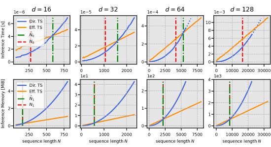
Figure 1: Inference time in seconds per image (top) and inference memory in MiB (bottom) of the attention mechanism (with $h=1$) vs. sequence length for both direct- (Dir. TS) and efficient-TaylorShift (Eff. TS). Each column uses a different internal dimension $d$. Additionally, we have marked the theoretical intersections $N_{0}$ and $N_{1}$, as well as the measured ones $\hat{N}_{0}$ and $\hat{N}_{1}$. The dotted lines extrapolate values by fitting a parabola.

5 Empirical Evaluation

We run a number of experiments that provide an empirical verification of our theoretical analysis of the transitional bounds, scalability, and required computational resources, as well as of the effective capacity of our proposed mechanism.

5.1 Efficiency of the TaylorShift module

To validate our theoretical analysis concerning the critical points $N_{0}$ and $N_{1}$, derived in Section 4, we conduct empirical tests on the runtime and memory requirements of both direct- and efficient-TaylorShift. For multiple internal dimensions $d$, we measure inference time and memory consumption of a single attention head ($h=1$) as the length $N$ of the input sequence increases.

In the upper row of Figure 1, we contrast the speed of efficient- and direct-TaylorShift. The quadratic growth in $N$ of the direct version and the linear growth of the efficient one are evident. Note that the difference between the theoretical $N_{0}$ and empirical $\hat{N}_{0}$ transition points $\hat{N}_{0}-N_{0}\approx 18d$ is approximately proportional to the internal dimension $d$. We hypothesize that the more sequential nature of efficient-TaylorShift results in more, costly reads and writes in GPU memory. In contrast, the parallelizable nature of direct-TaylorShift might exploit GPU resources more efficiently.

The plots for $d=62$ and $d=128$ appear incomplete due to increasing memory requirements for calculating subsequent steps of direct-TaylorShift, which is plotted in the second row. The expected inference time was extrapolated by fitting a parabola to the data. In the regimen of memory (second row of Figure 1), the theoretical and empirical intersections align closely $\hat{N}_{1}\approx N_{1}$, with an error of at most $0.6\%$. Comparing both rows shows efficient-TaylorShift becoming memory efficient earlier than it becomes efficient in terms of speed, highlighting the usefulness of efficient-TaylorShift in low-memory environments, in alignment with our theoretical results from Table 2. In the interval $[\hat{N}_{1},\hat{N}_{0}]$, it can be used to trade off time against memory.

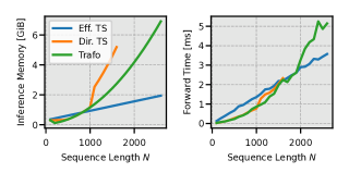
Figure 2: Memory and inference time of efficient- (Eff. TS) and direct-TaylorShift (Dir. TS) and the standard Transformer (Trafo) with $d=32$.

5.2 Efficiency of a Transformer with TaylorShift

We explore the efficiency of a full-scale Transformer encoder equipped with TaylorShift in Figure 2. At a sequence length of 900 tokens efficient-TaylorShift needs less memory and at 1800 tokens it surpasses the standard Transformer in speed. Note that at 1500 tokens it only needs half and at 2000 tokens only 35% of the Transformer’s memory. For shorter sequence length, direct-TaylorShift remains competitive with a standard Transformer in terms of speed and memory.

5.3 Performance of a Transformer with TaylorShift

Table 3: Accuracy in percent for models on datasets of different modalities. For the first three datasets, we closely adhere to the setup of (Tay et al., 2021). Models with ^⋆ had to be trained with full instead of mixed precision.

Model	CIFAR (Pixel)	IMDB (Byte)	ListOps	ImageNet (Ti)	ImageNet (S)	Average
Linformer	29.2	58.1	-	64.3	76.3	(57.0)
Performer	34.2⋆	65.6⋆	35.4⋆	62.0⋆	67.1⋆	52.9
Reformer	44.8	63.9	47.6	73.6	76.2⋆	61.2
Nystromformer	49.4	65.6	44.5	75.0	78.3⋆	62.6
Transformer	44.7	65.8	46.0	75.6	79.1	62.2
Ours	47.6	66.0	45.6	75.0	79.3	62.7

To assess the effectiveness of TaylorShift, we evaluate it across various datasets representing different modalities using a Transformer-encoder architecture. We track the classification accuracy of a TaylorShift-equipped Transformer across five tasks.

Tasks

We train on three datasets introduced by Tay et al. (2021), especially designed to assess Transformer performance on long sequences with long-range dependencies. The first is a pixel-level CIFAR10 task, where 8-bit intensity values of grayscale images from CIFAR10 are encoded into a sequence of discrete symbols of length 1024. Shifting into the domain of text, the second task, IMDB Byte (Maas et al., 2011), is a classification task for text encoded at the character/byte level, resulting in sequences of 4000 tokens and a more challenging overall task. Thirdly, we employ the Long ListOps dataset of mathematical operations (Nangia & Bowman, 2018) encoded at the character level, for which we utilize a custom implementation to procedurally generate batches of sequences with consistent lengths from 500 to 2000. Beyond these synthetic tasks, we train for image classification on ImageNet (Deng et al., 2009), a prominent benchmark in computer vision. We train models at two sizes (Ti & S) to additionally explore the scaling behavior of our proposed architecture. Refer to Appendix C for model sizes and training hyperparameters. To speed up calculations, we utilize mixed-precision training whenever possible.

Table 3 shows our method’s consistent performance across all datasets. It surpasses all other linear scaling Transformers on a minimum of four out of five datasets. Note that those models marked with ^⋆ could only be trained using with full precision, slowing down training considerably. TaylorShift also outperforms the standard Transformer on three out of five tasks, remains competitive on the remaining two, and demonstrates good scalability with model size. We observe a notable increase of $4.3\%$ when transitioning from architecture size Ti to S on ImageNet, in contrast to $3.5\%$ for the standard Transformer. These findings highlight the robustness and competitiveness of TaylorShift across diverse datasets and modalities. Together with the favorable scaling behavior, these results highlight TaylorShift’s practicality when dealing with sequences.

5.4 Ablations

We conduct an ablation analysis, systematically dissecting three key components to establish their impact on the performance of TaylorShift.

Normalization

Table 4: Accuracy on the CIFAR Pixel task when ablating our novel normalization introduced in Section 3.3.

Model	direct	efficient
Plain impl.	47.1	-
impl. +norm.	46.8	46.8
impl. +norm. +output norm.	47.1	47.6

We train a Transformer equipped with TaylorShift and different stages of normalization to track the impact of our normalization scheme. Table 4 shows that without normalization, direct-TaylorShift (Section 3.1) demonstrates acceptable performance, while the efficient version (Section 3.2) fails to converge during training. We attribute this to numerical overflow in intermediate results. Upon introducing input normalization to the attention mechanism, efficient-TaylorShift becomes trainable, and both implementations achieve an accuracy of 46.8%, a slight decrease for direct-TaylorShift. Additionally, normalizing the output to a mean size of 1, results in a performance boost for both implementations, bringing them to the accuracy level observed for the direct version before.

Token Embedding

Table 5: Accuracy on different datasets when changing the token embedding from a linear layer to a 3-layer CNN.

Dataset	lin. embed.	conv. embed.	$\Delta$
CIFAR (Pixel)	47.1	51.1	4.0
IMDB (Byte)	66.0	86.3	20.3
ListOps	45.6	64.8	19.2
ImageNet (Ti)	75.0	77.1	2.1
ImageNet (S)	79.3	78.5	-0.8

To test an orthogonal angle influencing efficiency, we take a look at the initial token embedding, fed into a TaylorShift-equipped Transformer encoder. Table 5 contrasts accuracy when transitioning from linear token embedding to a 3-layer CNN for different tasks. Notably, incorporating the CNN-embedding yields large performance improvements in the sequence-based tasks, indicating a complementing effect of convolutions and TaylorShift. We did not employ the CNN-embedding in other experiments to preserve experimental comparability. However, including it is an easy and efficient way of increasing model performance with linear complexity, without having to change the main backbone architecture.

Number of attention heads $h$

Table 6: Accuracy, throughput (TB), and VRAM (Mem) usage of TaylorShift on the CIFAR Pixel task with different number of attention heads $h$. All models have $d_{\text{embed}}=256$ with $d=\frac{d_{\text{embed}}}{h}$ in the attention mechanism. Accuracy is measured using direct-TaylorShift.

$h$	Acc	direct		efficient
		TP	Mem	TP	Mem
	[%]	[ims/s]	[MiB@16]	[ims/s]	[MiB@16]
1	44.7	23847	327	417	2655
2	46.3	16565	339	1150	1353
4	47.1	12060	596	2975	840
8	47.5	7657	1111	5749	585
16	47.3	4341	2135	9713	459
32	46.9	2528	4187	14087	397
64	45.9	1235	8291	13480	125

Finally, we validate our insights from Section 4.3 by training a TaylorShift-equipped encoder with varying numbers of attention heads $h$, while maintaining the embedding dimension $d_{\text{embed}}$. Note that the number of parameters stays almost exactly constant, while the attention temperature per head ($\tau$) changes. The results in Table 6 align with our theoretical analysis, demonstrating an acceleration and less memory demands as the number of heads increases. Notably, increasing the number of heads often leads to increased accuracy while concurrently speeding up calculations and reducing memory. These efficiency gains will become more significant for sequences longer than 1025 tokens. Beyond the point where accuracy increases, we can still leverage additional heads to trade off accuracy against speed and memory, particularly advantageous for processing longer sequences.

6 Conclusion

We present TaylorShift, an attention mechanism that computes token-to-token interactions in linear time and space. We lay the theoretical groundwork for using TaylorShift by studying the exact transition points where it becomes efficient. Empirical validation of our analysis through classification experiments confirms the performance benefits of TaylorShift for long sequences. TaylorShift even outperforms a standard Transformer across diverse datasets and modalities by 0.5% on average. Furthermore, investigations into the number of attention heads reaffirm the efficiency gains predicted theoretically. The number of heads can be tuned to improve the model’s effective capacity, its speed, and reduce memory requirements, all at once. While efficient-TaylorShift is faster than a standard Transformer for long sequences, we can swap back to the interchangeable direct-TaylorShift variant to keep the model’s efficiency for short sequences. By adopting TaylorShift, it will be possible to tackle tasks featuring long sequences such as high-resolution image classification and segmentation, processing long documents, integrating data from multiple modalities, and dynamically encoding lengthy documents into a prompt-specific context for Large Language Models. Overall, our findings underscore the efficiency and versatility of TaylorShift, positioning it as a competitive and scalable option in the landscape of efficient attention-based models.

Societal Impact

This paper presents work whose goal is to advance the field of Machine Learning. One possible consequence of work on efficient ML is the usage of ML models on smaller devices, allowing users to keep their data private while also potentially reducing the carbon emissions that come with requiring a large GPU datacenter for inference. Other potential societal consequences of our work, we feel must be not specifically highlighted here.

Appendix A Mathematical Details

A.1 Derivation of $N_{0}$

Simplification of $N_{0}$:

$$N_{0} =\frac{4d^{3}+10d^{2}+8d+3}{4d+6}$$

$$=\frac{4d^{3}+6d^{2}}{4d+6}+\frac{4d^{2}+6d}{4d+6}+\frac{3d+3}{4d+6}$$

$$=d^{2}+d+\frac{1}{2}$$

A.2 Derivation of $\hat{h}_{0}$

To find $\hat{h}_{0}$, we want to find $d=\frac{d_{\text{embed}}}{h}\in\mathbb{R}$, such that

$$8d^{3}+10d^{2}=3$$ (8)

holds.

$$10z^{3}+11z^{2} =3$$

$$\xLeftrightarrow{d=x-\frac{5}{12}}10x^{3}-\frac{25}{6}x-\frac{199}{108} =$$

$$\Leftrightarrow x^{3}-\frac{25}{48}x-\frac{199}{864} =0$$

$$\xLeftrightarrow{x=y+\frac{25}{144y}}y^{3}-\frac{199}{864}+\frac{15625}{2985984}y^{-3} =0$$

$$\xLeftrightarrow{u=y^{3}|\cdot u}u^{2}-\frac{199}{864}u+\frac{15625}{2985984} =0.$$

The last equation has the solution

$$u=\frac{199+18\sqrt{74}}{1728}.$$

Then we can substitute $\alpha:=\sqrt[3]{199+18\sqrt{74}}$ and $u=y^{3}$ using $\zeta_{3}=e^{\frac{2}{3}i\pi}$ a third root of unity, to get

$$y =\frac{\zeta_{3}^{j}}{12}\alpha$$

$$\Rightarrow x =y+\frac{25}{144y}=\frac{\zeta_{3}^{j}}{12}\alpha+\frac{25}{12}\alpha^{-1}\zeta_{3}^{-j}$$

$$\Rightarrow d =x-\frac{5}{12}=\frac{\zeta_{3}^{j}}{12}\alpha+\frac{25}{12}\alpha^{-1}\zeta_{3}^{-j}-\frac{5}{12}$$

for $j=0,1,2$.

Now, by the property of the third roots of unity, we have $\operatorname{Im}\zeta_{3}^{j}=-\operatorname{Im}\zeta_{3}^{-j}$. Since $\alpha\neq\frac{25}{\alpha}$, $d$ is real if and only if $j=0$. Therefore, the only real solution to Equation 8 is

$$d=\frac{1}{12}\alpha+\frac{25}{12}\alpha^{-1}-\frac{5}{12}\approx 0.47.$$

A.3 Derivation of $\hat{h}_{1}$

The goal is to find the optimum number of attention heads which implicitly fulfills

$$0 =-2d^{3}-(N+1)d^{2}+N$$

$$\Leftrightarrow N =2d^{3}+(N+1)d^{2}=(2d+N+1)d^{2}\overset{d>0}{\geq}(N+1)d^{2}.$$

Therefore it holds

$$1>\frac{N}{N+1}\geq d^{2},$$

which implies $1>d=\frac{d_{\text{embed}}}{\hat{h}_{1}}$ and $\hat{h}_{1}>d_{\text{embed}}$.

A.4 Derivation of $N_{1}$

We have $hdN_{1}+2hN_{1}^{2}=hd^{2}(d+1)+2hdN_{1}+h(d+1)N_{1}+hd^{2}N_{1}$ by definition of $N_{1}$. Therefore

$$d^{2}(d+1)+2dN_{1}+(d+1)N_{1}+d^{2}N =dN+2N^{2}$$

$$\Leftrightarrow N^{2}-\frac{d^{2}+2d+1}{2}N-\frac{d^{3}+d^{2}}{2} =0,$$

which has two solutions. The larger of those being

$$N_{1} =\frac{1}{4}\left[d^{2}+2d+1+\sqrt{(d^{2}+2d+1)^{2}+8(d^{3}+d^{2})}\right]$$

$$=\frac{1}{4}\left[d^{2}+2d+1+\sqrt{d^{4}+12d^{3}+14d^{2}+4d+1}\right].$$

Since

$$(d^{2}+6d+1)^{2} =d^{4}+12d^{3}+38d^{2}+12d+1$$

$$\geq d^{4}+12d^{3}+14d^{2}+4d+1,$$

we have

$$N_{1}\leq\frac{1}{2}d^{2}+2d+\frac{1}{2}.$$

Appendix B Normalization & Numerical Behavior

B.1 Training Without Normalization

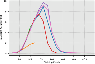
Figure 3: ImageNet accuracy in early training when using the efficient implementation without normalization during validation. These models have been trained at a sequence length of only $N=197$ using different hyperparameters.

We find that not using normalization leads to numerical instabilities during training. Large intermediate results quickly lead to degenerating performance due to numerical errors and training often breaks due to overflow-induced NaN-values. Figure 3 shows a few training runs, where normalization has been turned of at test time. These curves first displaying the influence of numerical inaccuracies while stopping after only a hand full of epochs, as numerical overflows render further calculations impossible. Our novel normalization scheme eliminates these types of training failures.

B.2 Scaling Behavior

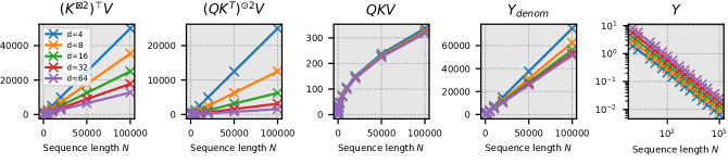
Figure 4: Mean norm of different expressions at sequence length $N$ from $1$ to $100000$ with ${Q,K,V\sim\text{unif}\left(\mathcal{S}^{d+1}\right)}$. Calculated using $16384$ samples each.

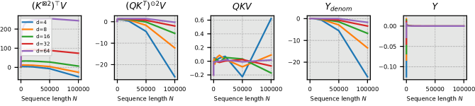
Figure 5: Absolute errors of our fitted scaling behaviors from Table 1 to empirical values in Figure 4.

To analyze the scaling behavior of TaylorShift and inform our normalization (see Section 3.3 in the main paper), take a look at the size of intermediate results of our calculations when varying $d$ and $N$. We uniformly sample the matrices $Q,K,V\in\mathbb{R}^{N\times d}$ from the unit sphere, as our formulation uses normalized queries and keys. We then measured the mean vector norm of intermediate results. Experimental results of the scaling behavior of intermediate expressions of our efficient implementation are shown in Figure 4. We have manually fitted the equations in Table 1 from this data. Figure 5 shows the errors of in these fitted functions. These errors are $\leq 1\%$ for large sequence length $N$, making our approximations useful for normalization.

Appendix C Experimental Setup

Table 7: Model sizes and training hyperparameters that were used for all models, depending on the dataset. These hyperparameters are based on (Touvron et al., 2022) for ImageNet and on (Tay et al., 2021) for the other datasets. The lr schedule, warmup epochs, weight decay, dropout, and drop path rate were the same for all models. We trained on NVIDIA A100 GPUs.

param	CIFAR (Pixel)	IMDB (Byte)	ListOps	ImageNet (Ti)	ImageNet (S)
model depth	1	4	4	12	12
$d_{\text{embed}}$	256	256	512	192	348
heads $h$	4	4	8	3	6
MLP ratio	1	4	2	4	4
lr	5e-4	5e-5	1e-3	3e-3
batch size	256	32	256	2048
epochs	200	200	200	300
lr schedule	cosine decay
warmup epochs	5
weight decay	1e-3
pos. embed.	cosine	cosine	cosine	learned
dropout	0
drop path rate	0.05
optimizer	fused LAMB
mixed precision	whenever possible
data augmentation	-	-	-	3-augment (Touvron et al., 2022)
GPUs	4	4	8	4/8	8

Table 7 shows the hyperparameters we used for training on the different datasets. Our hyperparameter choices and model sizes are based on (Tay et al., 2021) for the CIFAR, IMDB, and ListOps datasets and on (Touvron et al., 2022) for ImageNet. For IMDB and CIFAR, we used Byte-level encoding. ListOps is encoded at the character level (17 possible characters), and for ImageNet, we encoded RGB-patches of size $16\times 16$.

We did implement every attention mechanism using PyTorch at the same level of abstraction. In particular, we did not use any low-level implementation of the standard attention mechanism to ensure an even comparison. We consider such lower-level optimizations to be orthogonal to our analysis, as these can be done for all attention mechanisms.

Appendix D Further Analysis

D.1 Varying Sequence Length $N$

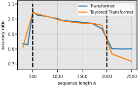
Figure 6: Ratio between the accuracy obtained on the test set and at a specific sequence lengths of the ListOps task. The training and test sets contain sequences of length 500 to 2000, marked by the black dashed lines.

We explore the performance of our model on sequences of varying length in Figure 6. For both the baseline and TaylorShift, accuracy gradually declines within the training distribution, spanning from 500 to 2000 tokens. We attribute this trend to the increasing complexity of solving mathematical operations as the number of operations grows. Outside the training distribution, accuracy drops rapidly to approximately $80\%$ of the test accuracy, with the accuracy of TaylorShift decreasing slightly more in this out-of-distribution setting.

References

- Babiloni et al. (2023) Babiloni, F., Marras, I., Deng, J., Kokkinos, F., Maggioni, M., Chrysos, G., Torr, P., and Zafeiriou, S. Linear complexity self-attention with 3rd order polynomials. IEEE Transactions on Pattern Analysis and Machine Intelligence, pp. 1–12, 2023. doi: 10.1109/tpami.2022.3231971.
- Banerjee et al. (2020) Banerjee, K., C., V. P., Gupta, R. R., Vyas, K., H., A., and Mishra, B. Exploring alternatives to softmax function. CoRR, abs/2011.11538, 2020.
- Bulatov et al. (2023) Bulatov, A., Kuratov, Y., and Burtsev, M. S. Scaling transformer to 1m tokens and beyond with rmt. 2023. doi: 10.48550/ARXIV.2304.11062.
- Choromanski et al. (2021) Choromanski, K. M., Likhosherstov, V., Dohan, D., Song, X., Gane, A., Sarlos, T., Hawkins, P., Davis, J. Q., Mohiuddin, A., Kaiser, L., Belanger, D. B., Colwell, L. J., and Weller, A. Rethinking attention with performers. In International Conference on Learning Representations, 2021.
- Dai et al. (2019) Dai, Z., Yang, Z., Yang, Y., Carbonell, J., Le, Q. V., and Salakhutdinov, R. Transformer-xl: Attentive language models beyond a fixed-length context. In Proceedings of the 57th Annual Meeting of the Association for Computational Linguistics, pp. 2978–2988, Florence, Italy, July 2019. Association for Computational Linguistics. doi: 10.18653/v1/P19-1285.
- Dass et al. (2023) Dass, J., Wu, S., Shi, H., Li, C., Ye, Z., Wang, Z., and Lin, Y. Vitality: Unifying low-rank and sparse approximation for vision transformer acceleration with a linear taylor attention. In 2023 IEEE International Symposium on High-Performance Computer Architecture (HPCA), pp. 415–428, Los Alamitos, CA, USA, mar 2023. IEEE Computer Society. doi: 10.1109/HPCA56546.2023.10071081.
- de Brébisson & Vincent (2016) de Brébisson, A. and Vincent, P. An exploration of softmax alternatives belonging to the spherical loss family. In Bengio, Y. and LeCun, Y. (eds.), 4th International Conference on Learning Representations, ICLR 2016, San Juan, Puerto Rico, May 2-4, 2016, Conference Track Proceedings, 2016.
- Deng et al. (2009) Deng, J., Dong, W., Socher, R., Li, L.-J., Li, K., and Fei-Fei, L. ImageNet: A large-scale hierarchical image database. In 2009 IEEE Conference on Computer Vision and Pattern Recognition. IEEE, 2009. doi: 10.1109/cvpr.2009.5206848.
- El-Nouby et al. (2021) El-Nouby, A., Touvron, H., Caron, M., Bojanowski, P., Douze, M., Joulin, A., Laptev, I., Neverova, N., Synnaeve, G., Verbeek, J., and Jegou, H. Xcit: Cross-covariance image transformers. In Beygelzimer, A., Dauphin, Y., Liang, P., and Vaughan, J. W. (eds.), Advances in Neural Information Processing Systems, 2021.
- Fournier et al. (2023) Fournier, Q., Caron, G. M., and Aloise, D. A practical survey on faster and lighter transformers. ACM Comput. Surv., 3 2023. ISSN 0360-0300. doi: 10.1145/3586074.
- Gaikwad & El-Sharkawy (2018) Gaikwad, A. S. and El-Sharkawy, M. Pruning convolution neural network (squeezenet) using taylor expansion-based criterion. In 2018 IEEE International Symposium on Signal Processing and Information Technology (ISSPIT). IEEE, 2018. doi: 10.1109/isspit.2018.8705095.
- Iwana et al. (2019) Iwana, B. K., Kuroki, R., and Uchida, S. Explaining convolutional neural networks using softmax gradient layer-wise relevance propagation. In Proceedings - 2019 International Conference on Computer Vision Workshop, ICCVW 2019, Proceedings - 2019 International Conference on Computer Vision Workshop, ICCVW 2019, pp. 4176–4185, United States, October 2019. Institute of Electrical and Electronics Engineers Inc. doi: 10.1109/ICCVW.2019.00513.
- Katharopoulos et al. (2020) Katharopoulos, A., Vyas, A., Pappas, N., and Fleuret, F. Transformers are rnns: Fast autoregressive transformers with linear attention. International Conference on Machine Learning, pp. 5156–5165, 2020.
- Keles et al. (2023) Keles, F. D., Wijewardena, P. M., Hegde, C., Keles, F. D., Wijewardena, P. M., and Hegde, C. On the computational complexity of self-attention. In International Conference on Algorithmic Learning Theory, pp. 597–619. PMLR, 2023.
- Lin et al. (2022) Lin, T., Wang, Y., Liu, X., and Qiu, X. A survey of transformers. AI Open, 3:111–132, 2022. ISSN 2666-6510. doi: 10.1016/j.aiopen.2022.10.001.
- Liu et al. (2021) Liu, Z., Lin, Y., Cao, Y., Hu, H., Wei, Y., Zhang, Z., Lin, S., and Guo, B. Swin transformer: Hierarchical vision transformer using shifted windows. In 2021 IEEE/CVF International Conference on Computer Vision (ICCV), pp. 9992–10002, Los Alamitos, CA, USA, 10 2021. IEEE Computer Society. doi: 10.1109/ICCV48922.2021.00986.
- Maas et al. (2011) Maas, A. L., Daly, R. E., Pham, P. T., Huang, D., Ng, A. Y., and Potts, C. Learning word vectors for sentiment analysis. In Lin, D., Matsumoto, Y., and Mihalcea, R. (eds.), Proceedings of the 49th Annual Meeting of the Association for Computational Linguistics: Human Language Technologies, pp. 142–150, Portland, Oregon, USA, June 2011. Association for Computational Linguistics.
- Molchanov et al. (2017) Molchanov, P., Tyree, S., Karras, T., Aila, T., and Kautz, J. Pruning convolutional neural networks for resource efficient inference. In International Conference on Learning Representations, 2017.
- Montavon et al. (2015) Montavon, G., Bach, S., Binder, A., Samek, W., and Müller, K.-R. Explaining nonlinear classification decisions with deep taylor decomposition. Pattern Recognition, 65:211–222, May 2015. ISSN 0031-3203. doi: 10.1016/j.patcog.2016.11.008.
- Nangia & Bowman (2018) Nangia, N. and Bowman, S. ListOps: A diagnostic dataset for latent tree learning. In Cordeiro, S. R., Oraby, S., Pavalanathan, U., and Rim, K. (eds.), Proceedings of the 2018 Conference of the North American Chapter of the Association for Computational Linguistics: Student Research Workshop, pp. 92–99, New Orleans, Louisiana, USA, June 2018. Association for Computational Linguistics. doi: 10.18653/v1/N18-4013.
- Nauen et al. (2023) Nauen, T. C., Palacio, S., and Dengel, A. Which transformer to favor: A comparative analysis of efficiency in vision transformers, 2023.
- Nivron et al. (2023) Nivron, O., Parthipan, R., and Wischik, D. Taylorformer: Probabalistic modelling for random processes including time series. In ICML Workshop on New Frontiers in Learning, Control, and Dynamical Systems, 2023.
- Qiu et al. (2023) Qiu, Y., Zhang, K., Wang, C., Luo, W., Li, H., and Jin, Z. Mb-taylorformer: Multi-branch efficient transformer expanded by taylor formula for image dehazing. In Proceedings of the IEEE/CVF International Conference on Computer Vision (ICCV), pp. 12802–12813, October 2023.
- Tay et al. (2021) Tay, Y., Dehghani, M., Abnar, S., Shen, Y., Bahri, D., Pham, P., Rao, J., Yang, L., Ruder, S., and Metzler, D. Long range arena: A benchmark for efficient transformers. In International Conference on Learning Representations, 2021.
- Tay et al. (2022) Tay, Y., Dehghani, M., Bahri, D., and Metzler, D. Efficient transformers: A survey. ACM Comput. Surv., 4 2022. doi: 10.1145/3530811.
- Touvron et al. (2022) Touvron, H., Cord, M., and Jégou, H. Deit iii: Revenge of the vit. In Avidan, S., Brostow, G., Cissé, M., Farinella, G. M., and Hassner, T. (eds.), Computer Vision – ECCV 2022, pp. 516–533, Cham, 2022. Springer Nature Switzerland.
- Tworkowski et al. (2023) Tworkowski, S., Staniszewski, K., Pacek, M., Wu, Y., Michalewski, H., and Miłoś, P. Focused transformer: Contrastive training for context scaling. In Thirty-seventh Conference on Neural Information Processing Systems. arXiv, 2023.
- Vaswani et al. (2017) Vaswani, A., Shazeer, N., Parmar, N., Uszkoreit, J., Jones, L., Gomez, A. N., Kaiser, L., and Polosukhin, I. Attention is all you need. In Guyon, I., Luxburg, U. V., Bengio, S., Wallach, H., Fergus, R., Vishwanathan, S., and Garnett, R. (eds.), Advances in Neural Information Processing Systems, volume 30. Curran Associates, Inc., 2017.
- Vincent et al. (2015) Vincent, P., de Brébisson, A., and Bouthillier, X. Efficient exact gradient update for training deep networks with very large sparse targets. Advances in Neural Information Processing Systems, 28, 2015.
- Wang et al. (2020) Wang, S., Li, B. Z., Khabsa, M., Fang, H., and Ma, H. Linformer: Self-attention with linear complexity, June 2020.
- Xing et al. (2020) Xing, C., Wang, M., Dong, C., Duan, C., and Wang, Z. Using taylor expansion and convolutional sparse representation for image fusion. Neurocomputing, 402:437–455, 2020. ISSN 0925-2312. doi: 10.1016/j.neucom.2020.04.002.
- Zaheer et al. (2020) Zaheer, M., Guruganesh, G., Dubey, A., Ainslie, J., Alberti, C., Ontanon, S., Pham, P., Ravula, A., Wang, Q., Yang, L., and Ahmed, A. Big bird: Transformers for longer sequences. In Proceedings of the 34th International Conference on Neural Information Processing Systems, NIPS’20, Red Hook, NY, USA, 2020. Curran Associates Inc. ISBN 9781713829546.
- Zhao et al. (2023) Zhao, H., Chen, Y., Sun, D., Hu, Y., Liang, K., Mao, Y., Sha, L., and Shao, H. Taylornet: A taylor-driven generic neural architecture, 2023.