Microscopic parametrization of the near threshold oscillations
of the nucleon time-like effective electromagnetic form factors

Abstract

We present an analysis of the recent near threshold BESIII data for the nucleon time-like effective form factors. The damped oscillation emerging from the subtraction of the dipole formula is treated in non-perturbative-QCD, making use of the light cone distribution amplitudes expansion. Non-perturbative effects are accounted for by considering $Q^{2}$-dependent coefficients in such expansions, whose free parameters are determined by fitting to the proton and neutron data. Possible implications and future analysis have been discussed.

I Introduction

The theoretical impossibility of describing the nucleon internal structure in terms of strongly interacting quarks and gluons, which are the fundamental fields of quantum chromodynamics, enhances the electromagnetic form factors (EMFFs) to the role of unique and privileged tools to unravel the dynamics underlying the electromagnetic interaction of nucleons. They provide the most effective description of the mechanisms that determine and rule the dynamic and static properties of nucleons. In specific reference frames, EMFFs represent the Fourier transforms of spatial charge and magnetic momentum densities.

Recently, the BESIII [1] experiment measured the time-like nucleon form factors (FFs) at center-of-mass energies between 2.0 GeV and 3.5 GeV [2, 3, 4, 5, 6]. These data present an oscillating behavior [7, 8, 9, 10, 11, 12], which manifests itself as a periodic, exponentially dumped component over the typical dipolar carrier, usually identified as the only contribution. The nature of such an oscillating component is still unknown. Possible explanations rely either on the final state interaction between the baryon and the antibaryon, or in a phenomenon intrinsic to the baryon structure. In the latter case, the invoked phenomenon would be encoded by the EMFFs of nucleons.

In order to investigate this eventuality we propose a parametrization for the EMFFs defined by considering the nucleons as triplets of collinear quarks lying at light-like distances in the light-front framework [13].

The matrix element of the “+” component of the hadronic current $J^{\mu}$, which depends directly on the EMFFs, evaluated between the baryon and antibaryon particle states, can then be expanded using the Lorentz invariance of the three quark Fock state’s matrix elements.

The resulting form depends on a set of functions of the four momentum squared fractions, called light cone distribution amplitudes (LCDAs), and a deep knowledge of their expression can provide further information about the form factors shape. Using the $\mathcal{L}_{\text{QCD}}$ conformal symmetry [14], the LCDAs are expanded on a polynomial basis, the most common choice being represented by the orthonormal Appell polynomials, defined on the triangle $T\left(x_{1},x_{3}\right)=\{\left(x_{1},x_{3}\right)\in\mathbb{R}:x_{1}>0,x_{3}>0,x_{1}+x_{3}<1\}$, where $x_{i}=k_{i}^{+}/P^{+}$ are the quark’s light front momentum fractions along is the $\left({}^{+}\right)$ direction and so the following relation holds: $\sum_{i=1}^{3}x_{i}=1$. The only unknown quantities now are the expansion coefficients, which have to be determined considering the phenomenology of the problem. The nonperturbative coefficients admit an evolution equation in the conformal symmetry framework, and their values can be determined theoretically by QCD sum rules. On the other hand, we are considering a center of mass energy of the system between 2.0 GeV and 3.5 GeV, so we are not allowed to use perturbative methods. What we propose then is to perform a truncated Laurent expansion of the non-perturbative coefficients over the negative powers of the four momentum squared, subsequently performing a fit over the recent BESIII experimental data to determine these coefficients. The final goal of this description is to find whether the oscillations of the EMFFs can be described by the model functions.

II The microscopic model

One of the most effective ways to describe subnuclear processes is to work on a light front framework, expanding the involved particle states in a free particle state basis, commonly known as Fock states. For a baryon we have

$$\left|{\rm baryon}\right\rangle=\left|0\right\rangle+\left|qqq\right\rangle+\left|qqqg\right\rangle+\left|qqqq\bar{q}\right\rangle+\dots\,,$$ (1)

where the three-quark state can be expanded in a Lorentz series of its matrix element between the vacuum and the particle states. The expansion has already been performed in Ref. [15], e.g., for the proton has the form

$$\left\langle 0\right|\varepsilon^{ijk}u^{i}_{\alpha}\left(a_{1}z\right)u^{j}_{\beta}\left(a_{2}z\right)d^{k}_{\gamma}\left(a_{3}z\right)\left|P\right\rangle$$ (2)

$$= \frac{1}{4}\Big{[}S_{1}MC_{\alpha\beta}\left(\gamma_{5}N^{+}\right)_{\gamma}+V_{1}\left(\not{p}C\right)_{\alpha\beta}\left(\gamma_{5}N^{+}\right)_{\gamma}\Big{.}$$

$$+P_{1}M\left(\gamma_{5}C\right)_{\alpha\beta}N_{\gamma}^{+}+A_{1}\left(\not{p}\gamma_{5}C\right)_{\alpha\beta}N_{\gamma}^{+}$$

$$\Big{.}+T_{1}\left(i\sigma_{\bot p}C\right)_{\alpha\beta}\left(\gamma^{\bot}\gamma_{5}N^{+}\right)_{\gamma}+\ldots\Big{]}\,,$$

where the functions $S_{1}$, $V_{1}$, $P_{1}$, $A_{1}$ and $T_{1}$ are called light cone distribution amplitudes, they are functions of the scalar product $P\cdot z$, $z$ being a light like four-vector. The dots in Eq. (2) indicate that the expansion has been written explicitly only for twist-3 LCDAs, while the complete expansion includes 24 LCDAs.

Considering now the whole expansion, we can find some conditions for the LCDAs imposing that the nucleon state isospin is 1/2. For example, for twist-3 LCDAs, the following equation holds

$$2T_{1}\left(x_{1},x_{2},x_{3}\right) = \left[V_{1}-A_{1}\right]\left(x_{1},x_{3},x_{2}\right)$$

$$+\left[V_{1}-A_{1}\right]\left(x_{2},x_{3},x_{1}\right)\,,$$

which allows to restrict the study of twist-3 LCDAs to a single function, which is chosen to be

$$\varphi_{N}\left(\mathbf{x}\right)=V_{1}\left(\mathbf{x}\right)-A_{1}\left(\mathbf{x}\right)\,,$$ (3)

where $\mathbf{x}$ is 3-vector $(x_{1},x_{2},x_{3})$. Taking advantage from the conformal symmetry of the Lagrangian density $\mathcal{L}_{\text{QCD}}$, the twist-3 LCDA $\varphi_{N}$ can be expanded over the orthonormalized Appell polynomials set $\left\{P_{n}\left(\mathbf{x}\right)\right\}_{n}$ as follows

$$\varphi_{N}\left(\mathbf{x},Q^{2}\right)=120x_{1}x_{2}x_{3}\sum_{n}B_{n}\left(Q^{2}\right)P_{n}\left(\mathbf{x}\right)\,.$$ (4)

The set of non-perturbative coefficients $\left\{B_{n}\right\}_{n}$ is unknown and contains all the information about the form factor for the leading twist.

Each coefficient $B_{n}$ is linked to the $\varphi_{N}$ LCDA’s momenta. The first coefficient $B_{0}$ is fixed being linked to the normalization of $\varphi_{N}$, i.e.,

$$B_{0}=\int_{0}^{1}dx_{1}\int_{0}^{1}dx_{2}\int_{0}^{1}dx_{3}\varphi_{N}\left(\mathbf{x},Q^{2}\right)=1\,.$$ (5)

As already stated, since we are considering the non perturbative aspect of the LCDAs, we can perform an expansion over the negative powers of the four-momentum squared,

$$B_{n}\left(Q^{2}\right)=\sum_{k=0}^{M_{n}}b_{k}^{\left(n\right)}Q^{-2k},$$ (6)

where $Q^{2}=-q^{2}$, $\left\{\{b_{k}^{(n)}\}_{k=0}^{M_{n}}\right\}_{n}$ is the set of coefficients and $M_{n}$ is the maximum power of $Q^{-2}$ in the expansion of the $n^{\rm th}$ parameter $B_{n}$.

III Leading order contributing diagrams

Taking the leading order into account, the minimum number of contributing diagrams has been evaluated in Ref. [15], where fourteen diagrams have been considered. The Sachs form factors which we are interested in are related to the Pauli and Dirac ones by the relations

$$G_{E}\left(Q^{2}\right) = F_{1}\left(Q^{2}\right)-\tau F_{2}\left(Q^{2}\right)\,,$$

$$G_{M}\left(Q^{2}\right) = F_{1}\left(Q^{2}\right)+F_{2}\left(Q^{2}\right)\,,$$

where $\tau=Q^{2}/\left(4M_{B}^{2}\right)$. We performed our fit over the effective form factor data, which is linked to the Sachs form factors by the relation

$$\left|G_{\text{eff}}\right|=\sqrt{\frac{\left|G_{E}\right|^{2}+2\tau\left|G_{M}\right|^{2}}{1+2\tau}}.$$

Following the works of Brodsky and Lepage [16], the light front EMFF can be written as the convolution of three probabilities, namely the probability of describing the baryon and antibaryon as a system of three collinear quarks, $\varphi_{N}\left(\mathbf{x},Q^{2}\right)$, and the probability of finding a certain strong interaction, known as hard scattering kernel $K_{H}$. At the leading order, each of the fourteen contributing diagrams corresponds to a hard scattering kernel $K_{i}\left(\mathbf{x},\mathbf{y}\right)$, here $\varphi_{N}\left(\mathbf{x}\right)=V_{1}\left(\mathbf{x}\right)-A_{1}\left(\mathbf{x}\right)$, and $T\left(\mathbf{x}\right)=T_{1}\left(\mathbf{x}\right)$ are the light cone distribution amplitudes involved in the calculation.

Table 1: Diagrams and leading twist baryon wave functions [15].

Index $i$	Diagram	$K_{i}(\mathbf{x},\mathbf{y})$
1		$\displaystyle\frac{\varphi_{N}(\mathbf{x})\varphi_{N}(\mathbf{y})+4T(\mathbf{x})T(\mathbf{y})}{(1-x_{1})^{2}x_{3}(1-y_{1})^{2}y_{3}}$
2		0
3		$\displaystyle\frac{-4T(\mathbf{x})T(\mathbf{y})}{x_{1}x_{3}(1-x_{2})y_{1}y_{3}(1-y_{1})}$
4		$\displaystyle\frac{\varphi_{N}(\mathbf{x})\varphi_{N}(\mathbf{y})}{x_{1}x_{3}(1-x_{3})y_{1}y_{3}(1-y_{1})}$
5		$\displaystyle\frac{-\varphi_{N}(\mathbf{x})\varphi_{N}(\mathbf{y})}{x_{2}x_{3}(1-x_{3})y_{2}y_{3}(1-y_{1})}$
6		0
7		$\displaystyle\left(\frac{1}{x_{1}y_{1}}+\frac{1}{x_{2}y_{2}}\right)\frac{\varphi_{N}(\mathbf{x})\varphi_{N}(\mathbf{y})}{(1-x_{3})^{2}(1-y_{3})^{2}}$
8		0
9		$\displaystyle\frac{\varphi_{N}(\mathbf{x})\varphi_{N}(\mathbf{y})+4T(\mathbf{x})T(\mathbf{y})}{(1-x_{1})^{2}x_{2}(1-y_{1})^{2}y_{2}}$
10		$\displaystyle\frac{\varphi_{N}(\mathbf{x})\varphi_{N}(\mathbf{y})+4T(\mathbf{x})T(\mathbf{y})}{(1-x_{1})^{2}x_{2}(1-y_{1})^{2}y_{2}}$
11		0
12		$\displaystyle\frac{-\varphi_{N}(\mathbf{x})\varphi_{N}(\mathbf{y})}{x_{1}x_{2}(1-x_{3})y_{1}y_{2}(1-y_{1})}$
13		$\displaystyle\frac{4T(\mathbf{x})T(\mathbf{y})}{x_{1}x_{2}(1-x_{1})y_{1}y_{2}(1-y_{2})}$
14		$\displaystyle\frac{-\varphi_{N}(\mathbf{x})\varphi_{N}(\mathbf{y})}{x_{1}x_{2}(1-x_{1})y_{1}y_{2}(1-y_{3})}$

In order to evaluate the form factor $G_{M}$, we used the Chernyak-Zhitnitsky [15] asymptotic formula

$$\displaystyle q^{4}G_{M}\left(q^{2}\right)\rightarrow\frac{\left(4\pi\bar{\alpha}_{s}\right)^{2}}{54}\left|f_{N}\right|^{2}$$

$$\displaystyle\int\!\!\left[dx\right]\!\!\int\!\!\left[dy\right]\left(2\sum_{i=1}^{7}e_{i}K_{i}\left(\mathbf{x},\mathbf{y}\right)+\!\sum_{i=8}^{14}e_{i}K_{i}\left(\mathbf{x},\mathbf{y}\right)\right)\,,$$ (7)

where $\left[dx\right]=\delta\left(1-\sum_{i=1}^{3}x_{i}\right)dx_{1}dx_{2}dx_{3}$ and $\bar{\alpha}_{s}$ is the modified coupling constant. For the evaluation of the modified coupling constant $\bar{\alpha}_{s}^{2}$, we follow the procedure proposed by Chernyak and Zhitnitsky in Ref. [15]. The value of $\bar{\alpha}_{s}^{2}$ is given by the product of the coupling constants for the two subprocesses, namely the two gluon exchanges which appear in the tree-level diagrams shown in Table 1. The average virtuality ${\bar{q}}_{1}^{2}$ of the lightest gluon is ${\bar{x}}_{3}{\bar{y}}_{3}q^{2}$, while the rest gluon has an averaged virtuality ${\bar{q}}_{2}^{2}=\overline{(1-x_{1})}\,\,\overline{(1-y_{1})}q^{2}$. The typical values of a realistic nucleon wave function for the ${\bar{x}}_{i}$ are ${\bar{x}}_{1}\simeq 2/3$, ${\bar{x}}_{2}\simeq{\bar{x}}_{3}\simeq 1/6$. Therefore $\bar{\alpha}_{s}^{2}\left(q^{2}\right)=\alpha_{s}\left(\frac{1}{36}q^{2}\right)\alpha_{s}\left(\frac{1}{9}q^{2}\right)$.

The integrals in Eq. (III) are (weakly) convergent, it is possible to solve them analytically. The results have already been obtained in Ref. [14], and are reported in Appendix C. Non-perturbative-QCD effects are accounted for by considering the $Q^{2}$-dependence of the $B_{n}$ defined in Eq. (6) as truncated expansions in powers of $Q^{-2}$. The first parameter $B_{0}$ is fixed to 1 and is related to the zero order of the LCDA $\varphi_{N}$, so it is considered a constant. As for the other parameters, we are for now limiting our discussion to the LCDA’s second order momenta, so we are only interested in the first six parameters, namely those of the set $\{B_{n}\}_{n=0}^{5}$.

For the truncated expansion, we propose $M_{0}=0$, $M_{1}=M_{2}=1$, $M_{3}=M_{4}=M_{5}=2$, so that

$$B_{0} = 1\,,$$

$$B_{n}(Q^{2}) = b_{0}^{(n)}+\frac{b_{1}^{(n)}}{Q^{2}}\,,\ \ \ n=1,2\,,$$

$$B_{m}(Q^{2}) = b_{0}^{(m)}+\frac{b_{1}^{(m)}}{Q^{2}}+\frac{b_{2}^{(m)}}{(Q^{2})^{2}}\,,\ \ \ m=3,4,5\,.$$ (8)

We obtain a closed expression of the form factor $G_{M}$ depending only on the non-perturbative parameters for the proton and the neutron. Since the nucleons are related by the isospin symmetry, their parameters are the same we can performed a simultaneous fit to the recent BESIII data on proton and neutron cross sections to determine the sets of coefficients $\left\{\{b_{k}^{(n)}\}_{k=0}^{M_{n}}\right\}_{n=0}^{5}$. The fit is performed using the ROOT Data Analysis Framework [17] program.

IV Results and discussion

Figure 1 shows the results for the effective proton (upper panel) and neutron (lower panel) form factors in comparison with the experimental values measured by the BESIII experiment [2, 3, 4]. The fit functions depend on 13 free parameters, which are the coefficients of the expressions of Eq. (8). The normalized minimum $\chi^{2}$ is

$$\frac{\chi^{2}}{n_{\rm DoF}}=\frac{79.93}{43}\simeq 1.79\,.$$

It has been obtained by using 48 data points of the proton cross section and 18 of the neutron one. The error bands have been determined by considering both the errors of data, and the theoretical systematic error of the model, which has ben estimated by using expressions for the $B_{n}(Q^{2})$ parameters with the additional power $\left(Q^{-2}\right)^{M_{n}+1}$.

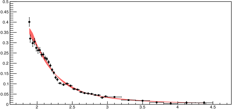
Figure 1: The bands represent the fit results for the proton (upper panel) and neutron (lower panel) effective form factor. The data are from the BESIII experiment [2, 3, 4].

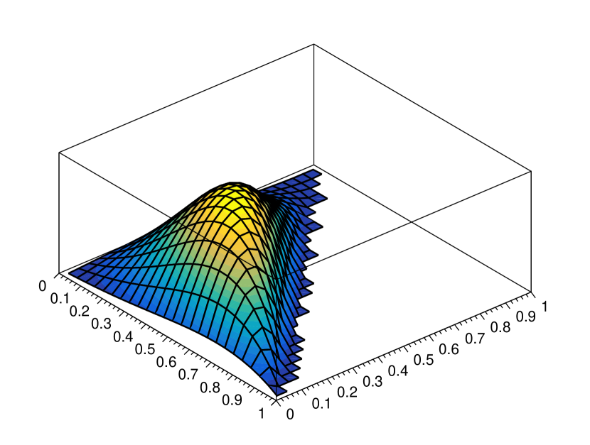
Figure 2: The nucleon distribution function $\varphi_{N}(\mathbf{x})$ obtained at $\sqrt{-Q^{2}}=2.5$ GeV as a function of $x_{1}$ and $x_{3}$.

Figure 2 shows the twist-3 nucleon distribution amplitude $\varphi_{N}(\mathbf{x})$ evaluated at $\sqrt{-Q^{2}}=2.5$ GeV. The maximum value is reached at the light-cone momentum fractions

$$x_{1}\simeq 0.49\,,\qquad x_{2}\simeq 0.24\,,\qquad x_{3}\simeq 0.27\,,$$ (9)

which agree with the assumption made in the Chernyak-Zhitnitsky formula [15] that the first quark has a momentum fraction about 50% larger than the other two, which equally divide the remaining momentum fraction.

Summarizing, a coherent model has been developed to reproduce the data on proton and neutron EMFFs, recently obtained by the BESIII collaboration. The model is based on a parameterization of the light-cone distribution amplitudes, and obeys conformal symmetry of the QCD Lagrangian.

The light-front quantization allows us to express the three-quark operator, occurring in the expression of the hard scattering kernel, as the Fourier transform of the light-cone distribution amplitudes, which, in turn, describe the behaviour of the three valence quarks constituting the baryon in a light-cone system. Always under the aegis of the QCD-Lagrangian conformal symmetry we expanded the leading-twist baryon distribution amplitudes over a set of Appell polynomials, which diagonalize the one gluon exchange kernel. The non-perturbative nature of the baryon distribution amplitudes is implemented by considering a $Q^{2}$-dependence of the expansion parameters $\left\{B_{n}\right\}_{n}$. We have restricted our calculations to the first six Appell polynomials.

These distribution amplitudes have been used to calculate the near threshold behaviour of the nucleon effective form factors, extending the valence of an asymptotic formula to the low-momentum transfer region. Such a near-threshold extension has been obtained by considering a $Q^{2}$-dependence of the expansion parameters $\left\{B_{n}(Q^{2})\right\}_{n}$, as polynomials of zero, first and second degree of $Q^{-2}$.

Moreover, since the nucleon EMFFs are linked by the isospin symmetry, the same set $\left\{B_{n}(Q^{2})\right\}_{n}$ can be used and the free coefficients of their power series can be determined by means a simultaneous fit to the proton and neutron data. The error bands of the near-threshold effective nucleon form factors, have been obtained by considering the experimental uncertainties of the data, used to determine the free parameters of the model and the theoretical systematic uncertainties due to the particular parametrization used.

This study aims to identify the origin or at least the dominant cause of the oscillatory behaviour of the effective nucleon form factors. In particular, we would like to distinguish between two hypotheses about the oscillation phenomenon: the intrinsic dynamical origin and the final state interaction. In the first case, the oscillations appear at the form factor level, while in the second case, they are due to re-scattering reactions that happen when the nucleons are already formed. A necessary condition in favour of the intrinsic origin is that there exists a microscopic model of nucleons that can give oscillatory form factors.

Even though for the neutron effective form factor the model reproduces quite well the oscillatory behaviour, it seems to fail in the case of the proton. Indeed, the obtained behaviour of the effective proton form factor, the orange band shown in the upper panel of Fig. 1, is compatible with the so-called regular background of Refs. [7, 8, 11]. It can be interpreted as the contribution due to the short distance quark-level dynamics [18, 19], i. e., the $p\bar{p}$ final state is produced by the creation of quark-antiquark pairs within a small volume, with a linear dimension much smaller than the standard hadron size of about 1 fm.

Nevertheless, the model has the added value of proving that a unique parametrization in all the kinematical ranges where data are present is effective both for proton and neutron FFs. This is in contrast to previous works, where a common fit could only be achieved either in a restricted kinematical region, concluding in a change of the phase [3], or at the price of three different models applicable in different kinematical regions [5].

Appendix A Contributing diagrams computation

Using the expressions [15]

$$\varphi_{N}(\mathbf{x}) = 120x_{1}x_{2}x_{3}\left(ax_{1}^{2}+bx_{2}^{2}+cx_{3}^{2}+dx_{3}+e\right)\,,$$

$$T(\mathbf{x}) = 120x_{1}x_{2}x_{3}\left[\frac{a+c}{2}\left(x_{1}^{2}+x_{2}^{2}\right)+bp_{3}^{2}+\right.$$ (10)

$$\left.\frac{d}{2}(1-x_{3})+e\right]\,,$$

where the values of the coefficients $a$, $b$, $c$, $d$, $e$ and $f$ are given in Ref. [15], the analytic solutions of the integrals of Eq. (III), namely the ten non-vanishing expressions

$${\cal K}_{i}=\int[dx]\int[dy]K_{i}(\mathbf{x},\mathbf{y})\,,$$ (11)

where the functions $K_{i}(\mathbf{x},\mathbf{y})$ are given in Table 1, with $i\in\{1,3,4,5,7,9,10,12,13,14\}$, are:

$${\cal K}_{1} = \left(I_{1}^{\left(1\right)}\right)^{2}+4\left(I_{1}^{\left(2\right)}\right)^{2}\,,$$

$$I_{1}^{(1)} = \frac{5}{12}(36a+6b+2c+12d+72e)\,,$$

$$I_{1}^{\left(2\right)} = \frac{5}{12}(21a+20b+3c+32d+72e)\,;$$ (12)

$${\cal K}_{3} = -4I_{3}^{(1)}I_{3}^{(2)}\,,$$

$$I^{(1)}_{3} = \frac{5}{3}(10a+2b+10c+15d+36e)\,,$$

$$I^{(2)}_{3} = \frac{5}{12}(15a+6b+15c+28d+72e)\,;$$ (13)

$${\cal K}_{4} = I_{4}^{(1)}I_{4}^{(2)}\,,$$

$$I_{4}^{(1)} = \frac{5}{2}(a+3b+2(c+2d+6e))\,,$$

$$I^{(2)}_{4} = \frac{5}{6}(6a+9b+3c+8d+36e)\,;$$ (14)

$${\cal K}_{5} = -I_{5}^{(1)}I_{5}^{(2)}\,,$$

$$I_{5}^{(1)} = \frac{5}{2}(3a+b+2(c+2d+6e))$$

$$I^{(2)}_{5} = \frac{10}{3}(9a+b+c+3d+18e)\,;$$ (15)

$${\cal K}_{7} = \left(I^{(1)}_{7}\right)^{2}+\left(I^{(2)}_{7}\right)^{2}\,,$$

$$I^{(1)}_{7} = \frac{5}{6}(a+3(b+6c+8d+12e))\,,$$

$$I^{(2)}_{7} = \frac{5}{6}(3a+b+6(3c+4d+6e))\,;$$ (16)

$${\cal K}_{9} = {\cal K}_{10}=\left(I^{(1)}_{9}\right)^{2}+4\left(I^{(2)}_{9}\right)^{2}\,,$$

$$I^{(1)}_{9} = \frac{5}{6}(18a+b+3c+8d+36e)\,,$$

$$I^{(2)}_{9} = \frac{5}{12}(19a+6b+19c+28d+72e)\,;$$ (17)

$${\cal K}_{12} = -I_{12}^{(1)}I_{12}^{(2)}\,;$$

$$I_{12}^{(1)} = \frac{10}{3}(a+b+9c+12d+18e)\,,$$

$$I_{12}^{(2)} = \frac{5}{6}(6a+3b+9c+16d+36e)\,;$$ (18)

$${\cal K}_{13} = 4I_{13}^{(1)}I_{13}^{(2)}$$

$$I_{13}^{(1)} = \frac{5}{12}(-3a+90b-3c+100d+360e)\,,$$

$$I_{13}^{(2)} = \frac{5}{12}(9a+18b+9c+20d+72e)\,;$$ (19)

$${\cal K}_{14} = -I_{14}^{(1)}I_{14}^{(2)}\,,$$

$$I_{14}^{(1)} = \frac{5}{6}(6a+3b+9c+16d+36e)\,,$$

$$I_{14}^{(2)} = \frac{10}{3}(a+b+9c+12d+18e)\,.$$ (20)

Appendix B Distribution amplitudes computation

B.1 Quark distribution amplitudes complex conjugate computation

Omitting the color and current indices, there is a proportionality between the hadronic current matrix element and the quark distribution amplitudes, given by

$$\left\langle P^{\prime}\right|\!J\!\left|P\right\rangle\propto\left\langle P^{\prime}\right|\!\bar{u}_{\mu}\bar{u}_{\nu}\bar{d}_{\rho}\!\left|0\right\rangle\left\langle 0\right|\!K_{H}^{\mu\nu\rho\alpha\beta\gamma}\!\left|0\right\rangle\left\langle 0\right|\!u_{\alpha}u_{\beta}d_{\gamma}\!\left|P\right\rangle,$$ (21)

so that the transition amplitude is proportional to the vacuum expectation value of the hard scattering kernel. The Feynman diagram is depicted in Fig. 3.

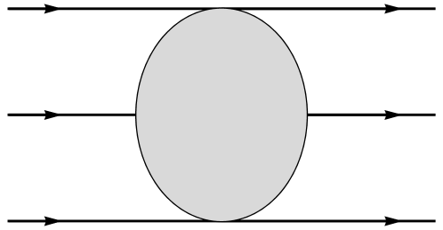
Figure 3: Basic graph for the hard scattering kernel.

The hard scattering structure $K_{H}^{\mu\nu\rho\alpha\beta\gamma}$ is given by a product of the three Lorentz structures which give the coupling of the three fermion lines:

$$K_{H}^{\mu\nu\rho\alpha\beta\gamma}=\Gamma_{1}^{\alpha\mu}\Gamma_{2}^{\beta\nu}\Gamma_{3}^{\gamma\rho}\,.$$ (22)

First of all, we need to write the complex conjugate of the matrix element representing the distribution amplitude $\varphi_{N}\left(\mathbf{x}\right)$. We calculate this directly as we can take the complex conjugate of the three parts composing the matrix element expansion:

$$\left\langle 0\right|u_{\alpha}u_{\beta}d_{\gamma}\left|P\right\rangle^{*} = \left\langle P\right|d^{\dagger}_{\gamma}u^{\dagger}_{\beta}u^{\dagger}_{\alpha}\left|0\right\rangle$$ (23)

$$= \left\langle P\right|\bar{d}_{i}\bar{u}_{j}\bar{u}_{k}\left|0\right\rangle\gamma^{0}_{i\gamma}\gamma^{0}_{j\beta}\gamma^{0}_{k\alpha}\,.$$

For the axial component we have

$$\left\langle P\right|\bar{d}_{i}\bar{u}_{j}\bar{u}_{k}\left|0\right\rangle_{A} = A_{1}^{*}\left(\not{P}\gamma_{5}C\right)^{*}_{\alpha\beta}N\left(P\right)^{*}_{\gamma}\gamma^{0}_{\gamma i}\gamma^{0}_{\beta j}\gamma^{0}_{\alpha k}$$ (24)

$$= A_{1}^{*}\left(\left(\not{P}\gamma_{5}C\right)^{\dagger}\right)_{\beta\alpha}\bar{N}\left(P\right)_{i}\gamma^{0}_{\beta j}\gamma^{0}_{\alpha k}$$

$$= A_{1}^{*}\left(C\gamma_{5}\not{P}\right)_{jk}\bar{N}\left(P\right)_{i}\,,$$

for the vector one

$$\left\langle P\right|\bar{d}_{i}\bar{u}_{j}\bar{u}_{k}\left|0\right\rangle_{V} = V_{1}^{*}\left(\not{P}C\right)^{*}_{\alpha\beta}\left(\gamma_{5}N\left(P\right)\right)^{*}_{\gamma}\gamma^{0}_{\gamma i}\!\gamma^{0}_{\beta j}\gamma^{0}_{\alpha k}$$ (25)

$$= -V_{1}^{*}\left(\left(\not{P}C\right)^{\dagger}\right)_{\beta\alpha}\left(\bar{N}\left(P\right)\gamma_{5}\right)_{i}\gamma^{0}_{\beta j}\gamma^{0}_{\alpha k}$$

$$= -V_{1}^{*}\left(C\not{P}\right)_{jk}\left(\bar{N}\left(P\right)\gamma_{5}\right)_{i}\,,$$

and finally for the tensorial part

$$\left\langle P\right|\bar{d}_{i}\bar{u}_{j}\bar{u}_{k}\left|0\right\rangle_{T} = T_{1}^{*}\left(\tensor{\sigma}^{\mu\nu}P_{\nu}C\right)^{*}_{\alpha\beta}\left(\gamma_{\mu}\gamma_{5}N\left(P\right)\right)^{*}_{\gamma}$$

$$\gamma^{0}_{\gamma i}\gamma^{0}_{\beta j}\gamma^{0}_{\alpha k}$$

$$= -T_{1}^{*}\left(\left(\tensor{\sigma}^{\mu\nu}P_{\nu}C\right)^{\dagger}\right)_{\beta\alpha}\left(\bar{N}\left(P\right)\gamma_{5}\gamma_{\mu}\right)_{i}$$

$$\gamma^{0}_{\beta j}\gamma^{0}_{\alpha k}$$

$$= -T_{1}^{*}\left(CP_{\nu}\tensor{\sigma}^{\mu\nu}\right)_{jk}\left(\bar{N}\left(P\right)\gamma_{5}\gamma_{\mu}\right)_{i}\,.$$

B.2 Distribution amplitudes convolutions

Here we compute the convolution of the distribution amplitudes used for the evaluation of the contributing diagrams. In each of the following calculations we use the anti-commutative properties of the gamma matrices, in particular the fact that the $\gamma_{5}$ matrix anti commutes with every component of the matrix four-vector $\gamma^{\mu}$, while for the charge conjugation matrix $C$ the following rule holds:

$$C\gamma^{\mu}C=-\left(\gamma^{\mu}\right)^{T}\,.$$ (27)

The axial, vector, tensor, and axial-vector components of the hadronic-current matrix element are, respectively,

$$\left\langle P^{\prime}\right|\!J\!\left|P\right\rangle_{A}\!\! = \!\left\langle P^{\prime}\right|\!\bar{u}_{\mu}\bar{u}_{\nu}\bar{d}_{\rho}\!\left|0\right\rangle_{A}\!\left\langle 0\right|\!K_{H}^{\mu\nu\rho\alpha\beta\gamma}\!\left|0\right\rangle\!\left\langle 0\right|\!u_{\alpha}u_{\beta}d_{\gamma}\!\left|P\right\rangle_{A}$$ (28)

$$= A_{1}^{*}\left(C\gamma_{5}\not{P}^{\prime}\right)_{\mu\nu}\left(\bar{N}P^{\prime}\right)_{\rho}\Gamma_{1}^{\mu\alpha}\Gamma_{2}^{\nu\beta}\Gamma_{3}^{\rho\gamma}A_{1}$$

$$\left(\not{P}\gamma_{5}C\right)_{\alpha\beta}N\left(P\right)_{\gamma}$$

$$= \left|A_{1}\right|^{2}\bar{N}\left(P^{\prime}\right)\Gamma_{3}N\left(P\right)$$

$$\left[-\Gamma_{1}^{\mu\alpha}\left(\not{P}\gamma_{5}C\right)_{\alpha\beta}\left(\Gamma_{2}^{T}\right)^{\beta\nu}\left(C\gamma_{5}\not{P}^{\prime}\right)_{\nu\mu}\right]$$

$$= -\left|A_{1}\right|^{2}\bar{N}\left(P^{\prime}\right)\Gamma_{3}N\left(P\right)$$

$$\text{Tr}\left[\Gamma_{1}\not{P}\gamma_{5}C\Gamma_{2}^{T}C\gamma_{5}\not{P}^{\prime}\right]$$

$$= \left(-1\right)^{1+2n_{2}}\left|A_{1}\right|^{2}\bar{N}\left(P^{\prime}\right)\Gamma_{3}N\left(P\right)$$

$$\text{Tr}\left[\Gamma_{1}\not{P}\overset{\leftrightarrow}{\Gamma}_{2}\not{P}^{\prime}\right]\,;$$

$$\left\langle P^{\prime}\right|\!J\!\left|P\right\rangle_{V}\!\! = \!\left\langle P^{\prime}\right|\!\bar{u}_{\mu}\bar{u}_{\nu}\bar{d}_{\rho}\!\left|0\right\rangle_{V}\!\left\langle 0\right|\!K_{H}^{\mu\nu\rho\alpha\beta\gamma}\!\left|0\right\rangle\left\langle 0\right|\!u_{\alpha}u_{\beta}d_{\gamma}\!\left|P\right\rangle_{V}$$ (29)

$$= -V_{1}^{*}\left(C\not{P}^{\prime}\right)_{\mu\nu}\left(\bar{N}\left(P^{\prime}\right)\gamma_{5}\right)_{\rho}\Gamma_{1}^{\mu\alpha}\Gamma_{2}^{\nu\beta}\Gamma_{3}^{\rho\gamma}$$

$$V_{1}\left(\not{P}C\right)_{\alpha\beta}\left(N\left(P\right)\gamma_{5}\right)_{\gamma}$$

$$= \left(-1\right)^{1+n_{3}}\left|V_{1}\right|^{2}\bar{N}\left(P^{\prime}\right)\Gamma_{3}N\left(P\right)$$

$$\left[\left(\Gamma_{1}\right)_{\mu\alpha}\left(\not{P}C\right)_{\alpha\beta}\left(\Gamma_{2}^{T}\right)_{\beta\nu}\left(C\not{P}^{\prime}\right)_{\nu\mu}\right]$$

$$= \left(-1\right)^{1+n_{3}}\left|V_{1}\right|^{2}\bar{N}\left(P^{\prime}\right)\Gamma_{3}N\left(P\right)$$

$$\text{Tr}\left[\Gamma_{1}\not{P}C\Gamma_{2}^{T}C\not{P}^{\prime}\right]$$

$$= \left(-1\right)^{1+n_{2}+n_{3}}\left|V_{1}\right|^{2}\bar{N}\left(P^{\prime}\right)\Gamma_{3}N\left(P\right)$$

$$\text{Tr}\left[\Gamma_{1}\not{P}\overset{\leftrightarrow}{\Gamma}_{2}\not{P}^{\prime}\right]$$

$$= -\left|V_{1}\right|^{2}\bar{N}\left(P^{\prime}\right)\Gamma_{3}N\left(P\right)\text{Tr}\left[\Gamma_{1}\not{P}\overset{\leftrightarrow}{\Gamma}_{2}\not{P}^{\prime}\right]\,;$$

$$\left\langle P^{\prime}\right|\!J\!\left|P\right\rangle_{T}\!\! = \!\!\left\langle P^{\prime}\right|\!\bar{u}_{\mu}\bar{u}_{\nu}\bar{d}_{\rho}\!\left|0\right\rangle_{T}\!\left\langle 0\right|\!K_{H}^{\mu\nu\rho\alpha\beta\gamma}\!\left|0\right\rangle\!\left\langle 0\right|\!u_{\alpha}u_{\beta}d_{\gamma}\!\left|P\right\rangle_{T}$$ (30)

$$= T_{1}^{*}\left(CP^{\prime}_{\lambda}\tensor{\sigma}^{\delta\lambda}\right)_{\mu\nu}\left(\bar{N}\left(P^{\prime}\right)\gamma_{5}\gamma_{\delta}\right)_{\rho}\Gamma_{1}^{\mu\alpha}\Gamma_{2}^{\nu\beta}\Gamma_{3}^{\rho\gamma}$$

$$T_{1}\left(\tensor{\sigma}^{\eta\kappa}P_{\kappa}C\right)_{\alpha\beta}\left(\gamma_{\eta}\gamma_{5}\left(N\left(P\right)\right)\right)_{\gamma}$$

$$= \left|T_{1}\right|^{2}P_{\lambda}^{\prime}P_{\kappa}\bar{N}\left(P^{\prime}\right)\gamma_{\delta}\Gamma_{3}\gamma_{\eta}N\left(P\right)$$

$$\left[\Gamma_{1}^{\mu\alpha}\left(\tensor{\sigma}^{\eta\kappa}C\right)_{\alpha\beta}\left(\Gamma_{2}^{T}\right)_{\beta\nu}\left(C\tensor{\sigma}^{\delta\lambda}\right)_{\nu\mu}\right]$$

$$= \left|T_{1}\right|^{2}P_{\lambda}^{\prime}P_{\kappa}\bar{N}\left(P^{\prime}\right)\gamma_{\delta}\Gamma_{3}\gamma_{\eta}N\left(P\right)$$

$$\text{Tr}\left[\Gamma_{1}\tensor{\sigma}^{\eta\kappa}C\Gamma_{2}^{T}C\tensor{\sigma}^{\delta\lambda}\right]$$

$$= \left|T_{1}\right|^{2}P_{\lambda}^{\prime}P_{\kappa}\bar{N}\left(P^{\prime}\right)\gamma_{\delta}\Gamma_{3}\gamma_{\eta}N\left(P\right)$$

$$\text{Tr}\left[\Gamma_{1}\tensor{\sigma}^{\eta\kappa}\overset{\leftrightarrow}{\Gamma}_{2}\tensor{\sigma}^{\delta\lambda}\right]\,;$$

$$\left\langle P^{\prime}\right|\bar{u}_{\mu}\bar{u}_{\nu}\bar{d}_{\rho}\left|0\right\rangle_{A}\left\langle 0\right|K_{H}^{\mu\nu\rho\alpha\beta\gamma}\left|0\right\rangle\left\langle 0\right|u_{\alpha}u_{\beta}d_{\gamma}\left|P\right\rangle_{V}$$

$$+\left\langle P^{\prime}\right|\bar{u}_{\mu}\bar{u}_{\nu}\bar{d}_{\rho}\left|0\right\rangle_{V}\left\langle 0\right|K_{H}^{\mu\nu\rho\alpha\beta\gamma}\left|0\right\rangle\left\langle 0\right|u_{\alpha}u_{\beta}d_{\gamma}\left|P\right\rangle_{A}$$

$$= \Big{[}A_{1}^{*}\left(C\gamma_{5}\not{P}^{\prime}\right)_{\mu\nu}\left(\bar{N}\left(P^{\prime}\right)\right)_{\rho}V_{1}\left(\not{P}C\right)_{\alpha\beta}\left(N\left(P\right)\gamma_{5}\right)_{\gamma}\Big{.}$$

$$\Big{.}-V_{1}^{*}\left(C\not{P}^{\prime}\right)_{\mu\nu}\!\left(\bar{N}\left(P^{\prime}\right)\gamma_{5}\right)_{\rho}A_{1}\!\!\left(\not{P}\gamma_{5}C\right)_{\alpha\beta}N\left(P\right)_{\gamma}\!\Big{]}$$

$$\Gamma_{1}^{\mu\alpha}\Gamma_{2}^{\nu\beta}\Gamma_{3}^{\rho\gamma}$$

$$= -\left(V_{1}A_{1}^{*}+V_{1}^{*}A_{1}\right)\bar{N}\left(P^{\prime}\right)\Gamma_{3}\gamma_{5}N\left(P\right)\text{Tr}\left[\Gamma_{1}\not{P}\overset{\leftrightarrow}{\Gamma}_{2}\not{P}^{\prime}\right]\,.$$

Appendix C Contributing diagrams in terms of the non-perturbative parameters

Here we write the integrals used for the calculation of the nucleon form factors $G_{M}^{p,n}$. The Chernyak-Zhitnitsky formula is

$$q^{4}G_{M}^{p,n}\left(q^{2}\right)\rightarrow\frac{\left(4\pi\bar{\alpha}_{s}\right)^{2}}{54}\left|f_{N}\right|^{2}I^{p,n}\,,$$ (32)

where the integrals $I^{p,n}$ up to the second degree polynomials are

$$I^{p} = 1400B_{0}B_{1}+\frac{2000}{9}B_{1}^{2}+1800B_{0}B_{2}+\frac{2800}{3}B_{1}B_{2}$$

$$+1200B_{2}^{2}+6600B_{0}B_{3}+\frac{22000}{9}B_{1}B_{3}+4800B_{2}B_{3}$$

$$+\frac{18800}{3}B_{3}^{2}-\frac{1000}{3}B_{0}B_{4}-\frac{2600}{27}B_{1}B_{4}-\frac{2200}{9}B_{2}B_{4}$$

$$-\frac{4600}{9}B_{3}B_{5}+\frac{2600}{243}B_{4}^{2}-1400B_{0}B_{5}-\frac{3500}{9}B_{1}B_{5}$$

$$-\frac{1100}{3}B_{2}B_{5}-\frac{5900}{3}B_{3}B_{5}+\frac{4100}{81}B_{4}B_{5}+\frac{7700}{27}B_{5}^{2}\,;$$

$$I^{n} = 1800B_{0}^{2}-1400B_{0}B_{1}+\frac{2000}{9}B_{1}^{2}-1800B_{0}B_{2}$$ (33)

$$-\frac{2800}{3}B_{1}B_{2}-200B_{2}^{2}-1000B_{0}B_{3}-\frac{22000}{9}B_{1}B_{3}$$

$$-2000B_{2}B_{3}-\frac{17000}{9}B_{3}^{2}+\frac{1000}{3}B_{0}B_{4}-\frac{2600}{27}B_{1}B_{4}$$

$$+\frac{2200}{9}B_{2}B_{4}+\frac{4600}{9}B_{3}B_{5}+\frac{2600}{243}B_{4}^{2}+\frac{2000}{3}B_{0}B_{5}$$

$$+\frac{3500}{9}B_{1}B_{5}+\frac{500}{9}B_{2}B_{5}+\frac{6500}{9}B_{3}B_{5}-\frac{4100}{81}B_{4}B_{5}$$

$$-\frac{7250}{81}B_{5}^{2}\,,$$

where the coefficients $\left\{B_{n}\right\}_{n=0}^{5}$ are the ones appearing in the expansion of the LCDA $\varphi_{N}\left(\mathbf{x},Q^{2}\right)$, and their operative form is given in Eq. (8).