Abstract

Most of the current studies on autonomous vehicle decision-making and control tasks based on reinforcement learning are conducted in simulated environments. The training and testing of these studies are carried out under rule-based microscopic traffic flow, with little consideration of migrating them to real or near-real environments to test their performance. It may lead to a degradation in performance when the trained model is tested in more realistic traffic scenes. In this study, we propose a method to randomize the driving style and behavior of surrounding vehicles by randomizing certain parameters of the car-following model and the lane-changing model of rule-based microscopic traffic flow in SUMO. We trained policies with deep reinforcement learning algorithms under the domain randomized rule-based microscopic traffic flow in freeway and merging scenes, and then tested them separately in rule-based microscopic traffic flow and high-fidelity microscopic traffic flow. Results indicate that the policy trained under domain randomization traffic flow has significantly better success rate and calculative reward compared to the models trained under other microscopic traffic flows.

1 1 0 https://doi.org/ Autonomous vehicle decision and control through reinforcement learning with traffic flow randomization Title Yuan Lin , Antai Xie* and Xiao Liu Yuan Lin, Antai Xie and Xiao Liu Yuan Lin, Antai Xie and Xiao Liu Correspondence: 202220159307@mail.scut.edu.cn(A.X.)

1 Introduction

In recent years, autonomous vehicles have received increasing attention as they have the potential to free drivers from the fatigue of driving and facilitate safe and efficient road traffic Le Vine et al. (2015). With the development of machine learning, rapid progress has been made in the development of autonomous vehicles, where machine learning provides the possibility for vehicles to learn from traffic data and the environment. In particular, reinforcement learning, which enables vehicles to learn driving tasks through trial and error, continuously interacts with the environment and improves learned policies. Compared to supervised learning, reinforcement learning does not require manual labeling or supervision of sample data, thus it is widely attempted for decision-making and control tasks of autonomous vehicles Sallab et al. (2017); Hoel et al. (2018); Ye et al. (2019, 2020). However, reinforcement learning models require tens of thousands of trial-and-error iterations for policy learning, and real vehicles on the road can hardly withstand so many trials. Therefore, current mainstream research on autonomous driving with reinforcement learning focuses on using virtual driving simulators for simulation training of agents.

Lin et al. Lin et al. (2020) have utilized deep reinforcement learning within a driving simulator Simulation of Mobility (SUMO) to train autonomous vehicles, enabling them to merge safely and smoothly at conical on-ramps. Meanwhile, Peng et al. Peng et al. (2022) also employed deep reinforcement learning algorithms within the SUMO driving simulation software to train a model for lane-changing and car-following. They tested the model by reconstructing scenes using NGSIM data, and the results indicate that models based on reinforcement learning demonstrate higher efficacy than those based on rule-based approaches. Mirchevska et al. Mirchevska et al. (2017) used fitted Q-learning for high-level decision-making on a busy simulated highway. However, microscopic traffic flows of these studies are based on rule-based models, such as the Intelligent Driver Model (IDM) Treiber et al. (2000); Liu et al. (2021); Huang et al. (2022) and the MOBIL lane-changing model. These are mathematical models based on mathematical formulas and traffic flow theory Punzo and Simonelli (2005), so they have a few parameters with clear meanings. They tend to simplify vehicle motion behavior and do not consider the interaction and kinematic constraints of multiple vehicles. Since most autonomous driving tasks involve extensive interaction with other vehicles in dynamically changing scenes, the strategies learned by the agents are influenced by the micro-traffic flow within the driving simulators. Autonomous vehicles trained with reinforcement learning in such microscopic traffic flows may perform exceptionally well when tested in similar conditions. However, when the trained model is applied to different traffic flows or real-world traffic flows, their performance may significantly deteriorate, and they could even cause traffic accidents. This is due to the discrepancies between simulated and the real-world scenes.

For research on sim-to-real transfer, numerous methods have been proposed to date. For instance, robust reinforcement learning has been explored to develop strategies that account for the mismatch between simulated and real-world scenes Tessler et al. (2019). Meta-learning is another approach that seeks to learn adaptability to potential test tasks from multiple training tasks Wang et al. (2016). Additionally, the domain randomization method discussed in this article is acknowledged as one of the most extensively used techniques to improve the adaptability to real-world scenes Andrychowicz et al. (2020). Domain randomization relies on highly randomized simulations aimed at encompassing the true distribution of real-world data, in spite of the mismatches between the simulation and actuality. Sheckells et al. Sheckells et al. (2019) applied domain randomization to vehicle dynamics, using stochastic dynamic models within simulations to optimize the control strategies for vehicles maneuvering on elliptical tracks, subsequently applying these strategies to real vehicles. The experiments indicate that the strategy was able to maintain performance levels similar to those achieved in simulations, unlike those trained with the simplistic kinematic vehicle model. However, few studies apply domain randomization to microscopic traffic flows and investigate efficiency.

In recent years, many driving simulators have been moving towards more realistic scenes. For certain driving simulators, their objective is to minimize the gap between reality and simulation, so we can use them for validation. Generally, driving simulators can be divided into three categories Wenl et al. (2023). The first category is flow-based driving simulators (such as Vissim Fellendorf and Vortisch (2010), Aimsun Casas et al. (2010), SUMO Lopez et al. (2018)) and their microscopic traffic flow is the rule-based model.The second category is vehicle-based driving simulators (such as AirSim Shah et al. (2018), CARLA Dosovitskiy et al. (2017), MetaDrive Li et al. (2022)), where microscopic traffic flows are generated by manually editing trajectories or replaying vehicle trajectories from traffic datasets, consistent with actual vehicle behavior but unable to accurately reflect the interactivity of actual traffic scenes. The third category is data-based driving simulators (InterSim Sun et al. (2022), TrafficGen Feng et al. (2023)), which train neural network models by extracting vehicle motion characteristics from real-world traffic datasets and apply the models to microscopic traffic flows, thus the microscopic traffic flows are interactive. However, since datasets are usually discontinuous and small-scale scenes, these simulators cannot simulate for a long time, and simulation time is much longer than the first two categories due to the complexity of the models. As far as our paper is concerned, the driving simulator LimSim Wenl et al. (2023) can generate long-term interactive high-fidelity traffic flows by combining multiple modules, balancing the advantages and disadvantages of the microscopic traffic flows of the above three types of driving simulators.

This paper proposes a domain randomization method for microscopic traffic flows for reinforcement learning-based decision and control. On the basis of rule-based microscopic traffic flows, the parameters of the car-following model and lane-changing model are randomized with a Gaussian distribution, making the microscopic traffic flows more random and behaviorally uncertain, thus exposing the agent to a complex and variable driving environment during training. To compare the impact of different microscopic traffic flows on the decision-making and control of reinforcement learning-based autonomous vehicles, this paper will train and test agents using the microscopic traffic flow without randomization, the high-fidelity microscopic traffic flow, and the domain randomization traffic flow in freeway and merging scenes.

The rest of this paper is structured as follows: Section 2 introduces related microscopic traffic flows. Section 3 describes the proposed method. Section 4 presents the simulation experiment and the analysis of the results for freeway and merging scenes. Finally, conclusions are drawn in Section 5.

2 Microscopic Traffic Flow

The characteristic parameters of traffic flow represent the efficiency of road traffic. Microscopic traffic flow models take individual vehicles as the research subject and describe in detail the driving behaviors of vehicles, such as acceleration, overtaking, and lane changing.

2.1 Rule-Based Microscopic Traffic Flow

IDM car-following model and SL2015 lane-changing model are frequently used as benchmarks for comparison in numerous SUMO-based studies, and SL2015 has more parameters that affect driver behavior. Consequently, this paper utilizes IDM and SL2015 as the default car-following and lane-changing models for the SUMO default microscopic traffic flow. The following is a detailed introduction to them.

2.1.1 IDM Car-following Model

IDM was originally proposed by Treiber in Treiber et al. (2000), characterized by a minimal number of parameters with clear meanings, capable of describing various traffic states from free flow to complete congestion with a unified formulaic approach. The model takes the preceding vehicle’s speed, the ego vehicle’s speed, and the distance to the preceding vehicle as inputs to output the ego vehicle’s safe acceleration. The acceleration of the ego vehicle at each timestep:

$$\dot{v}=a\left[1-\left(\frac{v}{v_{0}}\right)^{\delta}-\left(\frac{s^{*}(v,\Delta v)}{s}\right)^{2}\right],$$ (1)

where $a$ represents the maximum acceleration of the ego vehicle, $v$ is the current speed of the ego vehicle, $v_{0}$ is the desired speed of the ego vehicle, $\delta$ is the acceleration exponent, $\Delta v$ is the speed difference between the ego vehicle and the preceding vehicle, $s$ is the current distance between the ego vehicle and the preceding vehicle, and $s^{*}(v,\Delta v)$ is the desired following distance. The desired distance is defined as follows:

$$s^{*}(v,\Delta v)=s_{0}+\max\left(0,v*T+\frac{v*\Delta v}{2\sqrt{ab}}\right),$$ (2)

where $s_{0}$ is the minimum gap, $T$ is the bumper-to-bumper time gap and $b$ represents the maximum deceleration.

2.1.2 SL2015 Lane-changing Model

SL2015 is SUMO’s latest lane-changing model. The safety distance required for the lane-changing process is calculated as follows:

$$d_{\text{lc,veh}}(t)=\left\{\begin{array}[]{ll}v_{\text{veh}}(t)*a_{1}+2l_{\text{veh}},&\text{if }v_{\text{veh}}(t)\leq v_{\text{c}},\\ v_{\text{veh}}(t)*a_{2}+2l_{\text{veh}},&\text{if }v_{\text{veh}}(t)>v_{\text{c}},\end{array}\right.$$ (3)

where $d_{\text{lc,veh}}(t)$ denotes the safety distance required for lane changing, $v_{\text{veh}}(t)$ represents the velocity of the vehicle at time $t$, $l_{\text{veh}}$ is the length of the vehicle, $a_{1}$ and $a_{2}$ are safety factors, which are generally set to 5 and 15, the threshold speed $v_{\text{c}}$ differentiates between urban roads and highways.

After meeting the safety distance criteria for lane changing, vehicles are predisposed to move forward rapidly. Therefore, they compute the potential gains from lane changing at every timestep to expedite their journey to the destination. The decision to execute a lane changing is determined by the cumulative gains. The benefit $b_{ln}(t)$ at time $t$ for changing lanes is calculated as follows:

$$b_{ln}(t)=\frac{v_{\text{safe}}(t,ln)-v_{\text{safe}}(t,lc)}{v_{\text{max}}(lc)},$$ (4)

where $v_{\text{safe}}(t,ln)$ is the safe velocity of the vehicle in the target lane at the next timestep, $v_{\text{safe}}(t,lc)$ is the safe velocity in the current lane, and $v_{\text{max}}(lc)$ is the maximum velocity allowed in the current lane. The goal here is to maximize the velocity difference, thereby increasing the benefit of changing lanes.

If the profit for the current timestep is greater than zero, then this profit will be added to the cumulative profit. Conversely, if the profit for the current timestep is less than zero, the cumulative profit will be halved to moderate the desire to change to the target lane. Lane changing is initiated when the cumulative profit exceeds a preset threshold. When there are lanes on both the left and right sides of the vehicle, the profits for the left and right lanes are calculated independently.

SL2015 lane-changing model incorporates four layers of lane-changing motivations that encourage vehicle lane-changing maneuvers at each timestep: Strategic Change, where a vehicle must change lanes to follow the next part of its route; Cooperative Change, which occurs when a vehicle assists another in successfully changing lanes under certain real-world conditions; Tactical Change, where a vehicle changes lanes to avoid following a slower-moving vehicle; and Obligatory Change, which takes place in regions where right-hand driving is practiced and the left lane is designated for overtaking, requiring drivers to vacate the lane when not overtaking. Additionally, the model considers the emotional state of drivers, with most being compelled to cooperate in lane changing due to the emotional disposition of other drivers. A driver’s impatience is not static but fluctuates with various conditions. Drivers who have to wait multiple times for a lane changing tend to be less patient than those who can change lanes smoothly. Rising impatience can lead to more aggressive driving behavior, and this impatient disposition can also trigger lane-changing actions. The threshold for maximum impatience can be set using the driving parameter lcTimeToImpatience. Whenever a vehicle’s lane changing is impeded, the level of impatience increases.

2.2 High-Fidelity Microscopic Traffic Flow

The study employs the LimSim driving simulation platform’s high-fidelity microscopic traffic flow. LimSim conducted simulations based on the Freeway B dataset from CitySim Zheng et al. (2022) and analyzed the speed and following distance distributions of the simulated results. The findings indicate that the traffic flow generated by LimSim closely resembles actual data with a normal distribution, sharing similar means and standard deviations. The high-fidelity microscopic traffic flow in LimSim is based on optimal trajectory in the Frenet frame. Within the circular area around the ego vehicle, the microscopic traffic flow is updated based on each optimal trajectory.

2.2.1 Trajectory Generation

In the Frenet coordinate system, the motion state of a vehicle can be described by the tuple $[s,\dot{s},\ddot{s},d,\dot{d},\ddot{d}]$, where $s$ represents the longitudinal displacement, $\dot{s}$ the longitudinal velocity, $\ddot{s}$ the lateral acceleration, $d$ represents the lateral displacement, $\dot{d}$ the lateral velocity, $\ddot{d}$ the latitudinal acceleration. Frenet coordinate system is widely used in local trajectory planning because it can decouple a vehicle’s two-dimensional motion into two one-dimensional motions. It obtains candidate trajectory sets from both lateral and longitudinal motions and then combines them to generate the final trajectory.

Lateral Trajectory Generation

The lateral trajectory curve can be expressed by the following fifth-order polynomial:

$$d(t)=a_{d0}+a_{d1}t+a_{d2}t^{2}+a_{d3}t^{3}+a_{d4}t^{4}+a_{d5}t^{5}.$$ (5)

The initial trajectory value is known as $D_{0}=[d_{0},\dot{d}_{0},\ddot{d}_{0}]$, and a complete polynomial trajectory can be determined once the target value $D_{1}=[d_{1},\dot{d}_{1},\ddot{d}_{1}]$ is specified. As vehicles travel on the road, they use the road centerline as the reference line for navigation, and the optimal state for vehicle travel should be moving parallel to the centerline, which means the target state would be $D_{1}=[d_{1},0,0]$. By combining different polynomial target values $d_{i}$ and $T_{j}$, the entire lateral trajectory set can be generated:

$$[d_{1},\dot{d}_{1},\ddot{d}_{1},T]_{ij}=[d_{i},0,0,T_{j}],\quad\text{for }i,j\in\mathbb{N},$$ (6)

where $T_{j}$ is the $j$-th polynomial segment, $d_{i}$ is the $i$-th initial lateral distance, the time interval for each polynomial segment is the same, and the lateral trajectory set can be adjusted by varying the number of sampling points and the sampling step size for lateral distance and time.

Longitudinal Trajectory Generation

In many situations, vehicles doesn’t need to maintain a specific position, but rather it should approximate an ideal speed. Therefore, the lateral trajectory curve can be expressed with a fourth-degree polynomial:

$$s(t)=a_{s0}+a_{s1}t+a_{s2}t^{2}+a_{s3}t^{3}+a_{s4}t^{4}.$$ (7)

The initial trajectory values are known as $S_{0}=[s_{0},\dot{s}_{0},\ddot{s}_{0}]$, and when the target values $S_{1}=[\dot{s}_{1},\ddot{s}_{1}]$ are determined, a complete polynomial trajectory can be obtained. By combining the target values $\dot{s}_{1}$ and $T_{j}$ of different polynomials, the entire longitudinal trajectory set can be generated as follows:

$$[\dot{s}_{1},\ddot{s}_{1},T]_{ij}=[[\dot{s}_{d}+\Delta\dot{s}_{i}],0,T_{j}],\quad\text{for }i,j\in\mathbb{N},$$ (8)

where $\dot{s}_{d}$ is ideal speed and $\Delta\dot{s}_{i}$ is the sampled velocity gap, $T_{j}$ represents the $j$-th segment of the polynomial, and $\dot{s}_{i}$ is the initial longitudinal velocity of the $i$-th segment, the time interval for each polynomial segment is the same. The set of longitudinal trajectories can be adjusted by varying the number of sampling points and the sampling step size for both longitudinal velocity and time.

2.2.2 Optimal Trajectory Selection

During the process of selecting the final trajectory, it is important to ensure the safe operation of the autonomous vehicle while also keeping the deviation of the vehicle’s travel trajectory from the reference line as small as possible Low et al. (2019). A smooth trajectory can ensure the comfort of the occupants in the autonomous vehicle during travel Cailhol et al. (2019). Meanwhile, We hope that the vehicle’s driving speed tends towards the reference speed. The cost function formula for trajectory selection is as follows:

$$C_{total}=C_{\text{smooth}}+C_{\text{stable}}+C_{\text{obs}}+C_{\text{guide}}+C_{\text{vel}}.$$ (9)

where $C_{\text{smooth}}$ is the cost of trajectory smoothness, $C_{\text{stable}}$ is the cost of vehicle stability, $C_{\text{obs}}$ is the cost of collision likelihood, $C_{\text{guide}}$ is the cost of trajectory deviation from the reference trajectory, and $C_{\text{vel}}$ is the cost of the speed difference from the desired speed.

We utilize the overall cost function from Equation (9) to evaluate the set of candidate trajectories in Section 2.2.1, and select the trajectory with the smallest cost as the final trajectory.

Vehicles within a 50-meter perception range of the ego vehicle will be subject to the Frenet optimal trajectory control mentioned in Section 2.2.2, with a trajectory being planned every 0.5 seconds and each trajectory having a duration of 5 seconds.

3 Domain Randomization for Rule-Based Models of Microscopic Traffic Flow

To simulate the diversity of driving styles of surrounding drivers in actual driving environments, and to cope with complex traffic scenes, thereby improving the ego vehicle’s capability to handle various situations with ease, we propose a method of randomizing traffic flow parameters. This method is based on randomizing model parameters in SUMO’s IDM car-following model and SL2015 lane-changing model. The randomized parameters are shown in the Table 1.

"$\delta$" is the acceleration exponent in Equation (1) and "$T$" is the bumper-to-bumper time gap in Equation (2), respectively. The larger the "$\delta$" or the smaller the "$T$", the more aggressive the vehicle’s car-following behavior becomes. These two parameters influence the distribution of vehicles and may generate traffic scenarios that are rarely observed in real-world scenes.

Both "lcSpeedGain" and "lcAssertive" are parameters of the SL2015 lane-changing model, with "lcSpeedGain" indicating the degree to which a vehicle is eager to change lanes to gain speed; the larger the value, the lower the threshold for lane-changing, resulting in more aggressive lane-changing behavior. "lcAssertive" is another parameter that significantly influences the driver’s lane-changing model Berrazouane et al. (2019); a lower "lcAssertive" value makes the vehicle more inclined to accept smaller lane-changing gaps, leading to more aggressive lane-changing behavior. "$a_{max}$", "$a_{min}$", and "$v_{max}$" are the upper and lower limits of vehicle acceleration and the upper limit of speed, respectively. We set a small range of variation to increase the diversity of vehicle distributions in traffic scenes.

To ensure the driver behavior remains within plausible limits, we have opted to randomize these parameters in proximity to their default settings, while manually prescribing the bounds within which they can fluctuate. These randomized parameters follow a Gaussian distribution within the interval $[s_{\text{min}},s_{\text{max}}]$, with parameters $s$: $(\mu,\sigma^{2})$, $s_{\text{min}}\leq s\leq s_{\text{max}}$. Here, $\mu$ is set to $(s_{\text{max}}+s_{\text{min}})/2$, and $\sigma$ is set to $(s_{\text{max}}-s_{\text{min}})/6$, adhering to the $3-\sigma$ rule. When each vehicle is generated, the probability that its randomized parameter value will fall within $[s_{\text{min}},s_{\text{max}}]$ is 99.73 %.

When each vehicle is initialized on the road, these domain randomization parameters are generated and assigned to it, thus establishing the domain randomization microscopic traffic flow.

Table 1: Domain randomization parameters.

Parameter	Default Value	Random Interval $\boldsymbol{[s_{\text{min}},s_{\text{max}}]}$
$\delta$	4	[3.5, 4.5]
$T$	1	[0.5, 1.5]
$a_{max}$	2.6	[1.8, 3.4]
$a_{min}$	4.5	[3.5, 5.5]
$v_{max}$	8.33	[7.33, 9.33]
lcSpeedGain	1	[0, 100]
lcAssertive	1	[1, 5]

4 Simulation Experiment

In this section, we create freeway and merging environments in the open-source SUMO driving simulator Krajzewicz et al. (2012) and control the communication between SUMO and the reinforcement learning environment via TraCI Wegener et al. (2008). The timestep for the agent to select actions and observe environment state is set at 0.1 seconds. We train the reinforcement learning-based self-driving vehicles under different micro traffic flows in the freeway and merging scenes, respectively, with the aim of exploring which of the micro traffic flows the agents trained under have better decision-making and control capabilities in lane changing or merging.

4.1 Merging

4.1.1 Merging Environment

A control zone for the merging vehicle is established, spanning 100 meters to the rear of the on-ramp’s merging point and 100 meters to the front on the main road, as depicted in Figure 1. The red vehicle, operating under reinforcement learning control, is tasked with executing a smooth and safe merging within the designated control area.

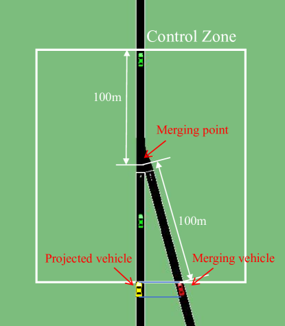
Figure 1: Merging in SUMO.

State

In defining the state of the reinforcement learning environment, the merging vehicle is projected onto the main road to produce the projected vehicle, and then a total of five vehicles are considered: two vehicles before the projected vehicle, two vehicles after the projected vehicle, and the projected vehicle. In order to utilize the observable information reasonably, the distance ($d^{p2}_{t},d^{p1}_{t},d^{f1}_{t},d^{f2}_{t},d^{m}_{t}$) of these five vehicles to the merging point, as well as their velocities ($v^{p2}_{t},v^{p1}_{t},v^{f1}_{t},v^{f2}_{t},v^{m}_{t}$), are included in the state representation. In addition, in order to take into account the comfort level of the present vehicle, we add the acceleration $a^{m}_{t}$ of the merging vehicle to the state.These parameters form a state representation with eleven variables, defined as:

$$s_{t}=[d^{p2}_{t},v^{p2}_{t},d^{p1}_{t},v^{p1}_{t},d^{m}_{t},v^{m}_{t},a^{m}_{t},d^{f1}_{t},v^{f1}_{t},d^{f2}_{t},v^{f2}_{t}]\in S.$$ (10)

Action

The action space we have defined is a continuous variable: acceleration within $[-4.5,2.5]\,m/s^{2}$. This range is consistent with the normal acceleration parameters of main-road vehicles, and it does not take into account velocities associated with emergency braking.

$$a_{t}=\{{acc^{m}_{t}}\}\in A.$$ (11)

Reward

We aim for the merging vehicle to maintain a safe distance from the preceding and following vehicles, ensure good comfort, and avoid coming to a stop or making the following vehicle brake sharply. Therefore, the reward function is expressed as follows:

$$R_{\text{total}}=R_{m}+R_{b}+R_{j}+R_{\text{stop}}+R_{\text{success}}+R_{\text{collision}}.$$ (12)

Within the control zone, the merging vehicle is safer when its projected position is between the preceding and following vehicles. The corresponding penalizing reward is defined as:

$$R_{m}=w_{m}*\left(|w|+\frac{\left|\displaystyle\frac{(v_{p1}+v_{f1})}{2}-v_{m}\right|}{\Delta v_{\text{max}}}\right),$$ (13)

where $w_{m}$ represents the weight factor, and $\Delta v_{\text{max}}$ is the maximum allowable speed difference. The variable $w$ is defined to measure the distance gap among the merging vehicle, its first preceding vehicle and its first following vehicle. The details are as follows:

$$w=\frac{\left|d_{p1}-d_{m}-l_{p1}\right|-\left|d_{m}-d_{f1}-l_{m}\right|}{\left|d_{p1}-d_{f1}-l_{p1}-l_{m}\right|},$$ (14)

where $l_{p1}$ and $l_{m}$ represent the lengths of the first preceding vehicle and the merging vehicle, both measuring 5 meters. When the first following vehicle performs braking in the control zone, a penalizing reward is defined as:

$$R_{b}=w_{b}\ast\frac{\left|a_{f1}\right|}{\max(\left|a_{\text{min}}\right|,a_{\text{max}})},$$ (15)

where $w_{b}$ is the weight and $a_{f1}$ is acceleration of the first following vehicle. In order to improve the comfort level of the merging vehicle, we define a penalizing reward for jerk:

$$R_{j}=w_{j}\ast\frac{\left|j_{m}\right|}{j_{\text{max}}}=-w_{j}\ast\frac{\left|\dot{a}_{m}\right|}{j_{\text{max}}},$$ (16)

where $w_{j}$ is the weight, $j_{\text{max}}$ is maximum allowed jerk and $\dot{a}_{m}$ is jerk of the merging vehicle.

In addition, if the merging vehicle comes to a stop, a penalty of $R_{\text{stop}}=-0.5$ is imposed. When a merged vehicle collides with any vehicle, a penalty of $R_{\text{collision}}=-1$ is applied. Conversely, if the merging vehicle successfully reaches its destination, a reward of $R_{\text{success}}=1$ is granted. Table 2 shows the values of the above mentioned parameters of the merging vehicle.

Table 2: Parameter values for the merging vehicle.

Parameter	Value
Weight for merging midway $w_{m}$	-0.015
Weight for penalizing first following’s braking $w_{b}$	-0.015
Weight for penalizing jerk $w_{j}$	-0.015
Maximum allowed speed difference $\Delta v_{\text{max}}$	$5\text{m/s}$
Maximum allowed jerk value $j_{\text{max}}$	$3\text{m/s}^{3}$

4.1.2 Soft Actor-Critic

Reinforcement learning is the approach that enables an agent to learn optimal decision-making and control through direct interaction with its environment. The SAC algorithm uses the classical framework of reinforcement learning, actor-critic, which helps to optimize the value function and the policy at the same time, and it consists of a parameterized soft-Q function $Q_{\theta}(\textbf{s}_{t},\textbf{a}_{t})$ and a tractable policy $\pi_{\phi}(a_{t}|s_{t})$. The parameters of these networks are $\theta$ and $\phi$. This approach Haarnoja et al. (2018) consider a more general maximum entropy objective which not only seeks to maximize rewards but also maintains a degree of randomness in action selection, as follows:

$$J(\pi)=\sum_{t=0}^{T}\mathbb{E}_{(\textbf{s}_{t},\textbf{a}_{t})\sim\rho_{\pi}}\gamma^{t}\left[r(\textbf{s}_{t},\textbf{a}_{t})+\alpha H(\pi(\cdot|\textbf{s}_{t}))\right],$$ (17)

in this context, $\rho_{\pi}$ denotes the state-action distribution under the policy $\pi$, while $H(\pi(\cdot|\mathbf{s}_{t}))$ signifies the entropy of the policy at state $\mathbf{s}_{t}$, thereby enhancing the unpredictability of the chosen actions. The temperature parameter $\alpha$ plays a pivotal role as it calibrates the balance between entropy and reward within the objective function, subsequently influencing the formulation of the optimal policy.

The merging environment has a continuous action space, so the agent is trained with the SAC algorithm. The hyperparameters of SAC is shown as follows:

Table 3: Hyperparameter values of SAC.

Parameter	Value
Reward discount factor	0.99
Optimizer	Adam
Actor network learning rate	0.001
Critic network learning rate	0.001
Experience replay memory size	1 000 000
Minibatch size	128
Actor network hidden layer size	$128\times 128$
Critic hidden layer size	$128\times 128$

4.1.3 Results Under Different Microscopic Traffic Flows

Training

In the merging environment, we trained 200,000 timesteps of 0.1s each in each of three different microscopic traffic flows. The training was carried out on an NVIDIA RTX 3060 graphics card paired with an Intel i7-12700F processor. It required 1 hours to complete the training using both SUMO’s default traffic flow and domain randomization traffic flow. In contrast, training with high-fidelity traffic flow took 3.5 hours.

Testing

The trained policy was tested an additional 1000 episodes in the freeway environment, and the ego vehicle merging at a vehicle vehicle generation probability of 0.56, consistent with the conditions during training. We evaluate the trained policy based on the merging vehicle’s success rate, which is defined by the completion of an episode without any collisions, and the average reward value over the entire testing period.

Comparison and Analysis

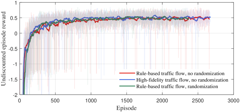
Figure 2: Undiscounted episode reward during training under three traffic flows.

Table 4: The results of testing three trained policies under three traffic flows in merging.

		Training
			$\mathbf{no\,randomization}$	$\mathbf{fidelity}$	$\mathbf{randomization}$
Testing	$\mathbf{no\,randomization}$	Average reward	0.0058	0.0002	-0.0018
		Success rate	98.50%	76.40%	91.60%
	$\mathbf{fidelity}$	Average reward	0.0029	0.0055	-0.0069
		Success rate	95.20%	97.50%	98.20%
	$\mathbf{randomization}$	Average reward	-0.0089	-0.0065	0.0057
		Success rate	56.00%	66.70%	99.30%

The training curves depicted in Figure 2 suggest that there is minimal difference in the rate of convergence and the rewards achieved by strategies trained under different microscopic traffic flows. Table 4 shows that the policy trained under microscopic traffic flow without randomization and high-fidelity microscopic traffic flow yield poor results when adapted to domain randomization traffic flow. Conversely, the policy trained under domain randomization microscopic traffic flows consistently achieve success rates above $90\%$ when tested across all three traffic flows, with a remarkable $99.3\%$ success rate under domain randomization traffic flow.

4.1.4 Test Results for Increasing Traffic Density

High-fidelity microscopic traffic flow closely resemble actual traffic scenes, so we use them as the test traffic flow, incrementally increasing traffic density. The impact of changes in traffic density is shown in Table 5, it can be observed that the policy trained under microscopic traffic flow without randomization experiences a gradual decline in success rate and rewards as traffic density increases. In contrast, the policy trained under domain randomization microscopic traffic flow consistently maintains a higher success rate, with both success rate and rewards remaining stable.

Table 5: The impact of changes in traffic density on three trained policies under the high-fidelity microscopic traffic flow.

		Traffic density for testing under high-fidelity traffic flow
			$\boldsymbol{\phi_{h}=0.56}$	$\boldsymbol{\phi_{h}=0.72}$	$\boldsymbol{\phi_{h}=0.89}$
Training with  rule-based traffic flow $(\boldsymbol{\phi=0.56})$	$\mathbf{no\,randomization}$	Average reward	0.0039	0.0017	0.0006
		Success rate	95.90%	93.30%	91.90%
	$\mathbf{randomization}$	Average reward	-0.0001	-0.0002	-0.0001
		Success rate	98.20%	98.50%	98.20%

* $\phi_{h}$ is the vehicle generation probability of high-fidelity microscopic traffic flow, defined as the number of vehicles that are generated from the starting point per second. $\phi$ is the vehicle generation probability of certain microscopic traffic flow.

4.2 Freeway

4.2.1 Freeway Environment

We used a straight, two-lane freeway measuring 1000 meters in length. Figure 3 depicts a standard lane-changing scenario in SUMO, where the ego vehicle is indicated by the red car and the surrounding vehicles are represented by the green cars. The green cars are set to three different traffic flows: microscopic flow without randomization, high-fidelity microscopic flow, and domain randomization microscopic flow.

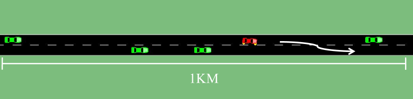
Figure 3: Freeway in SUMO.

State

The state of the environment is centered on the ego vehicle and four nearby vehicles: two directly in front and two directly behind it in the same lane, and two similarly positioned vehicles in adjacent lanes. At time $t$, the state is defined by the longitudinal distance ($d^{p}_{t},d^{f}_{t},d^{target_{p}}_{t},d^{target_{f}}_{t}$) of these four vehicles from the ego vehicle, their respective speeds ($v^{p}_{t},v^{f}_{t},v^{target_{p}}_{t},v^{target_{f}}_{t}$), and the speed and acceleration ($v^{ego}_{t},a^{ego}_{t}$) of the ego vehicle. These parameters form a state representation with ten variables as follows:

$$s_{t}=(d^{p}_{t},d^{f}_{t},d^{target_{p}}_{t},d^{target_{f}}_{t},v^{p}_{t},v^{f}_{t},v^{target_{p}}_{t},v^{target_{f}}_{t},v^{ego}_{t},a^{ego}_{t})\in S.$$ (18)

Action

The action space is defined as follows:

$$a_{t}=\{{acc^{ego}_{t},0,1}\}\in A,$$ (19)

where $acc^{ego}_{t}$ is a continuous action that indicates the acceleration of ego vehicle. Meanwhile, the discrete actions ’0’ and ’1’ dictate lane-changing behavior, the ’0’ means to keep the current lane and the ’1’ means an immediate lane changing to the other lane.

Reward

In reinforcement learning-based autonomous driving decision-making and control tasks, the purpose of rewards is to promote positive actions. Therefore, we have formulated a reward function aligned with practical driving objectives, incentivizing behaviors such as avoiding collisions, obeying speed limits, preserving comfortable driving conditions, and maintaining a safe following distance. The total reward is expressed as follows:

$$R_{\text{total}}=R_{\text{act}}+R_{\text{distance}}+R_{\text{jerk}}+R_{v}+R_{\text{collision}},$$ (20)

In order to penalize frequent lane changes, the penalty is defined as follows:

$$R_{\text{act}}=\begin{cases}\omega_{0},&\text{if }\left|y_{t-1}-y_{t}\right|\neq 0\text{ and }d^{p}_{t}<d_{\text{safe}},\\ \omega_{1},&\text{if }\left|y_{t-1}-y_{t}\right|\neq 0\text{ and }d^{p}_{t}>d_{\text{safe}},\\ 0,&\text{other},\end{cases}$$ (21)

where $y_{t}$ is ego vehicle’s lateral position and $\omega_{0}$ < $\omega_{1}$. If the vehicle changes lanes within the safety distance $d_{\text{safe}}$, it incurs a penalty of $\omega_{0}$. Alternatively, changing lanes outside $d_{\text{safe}}$ results in a penalty of $\omega_{1}$,

It is essential to ensure that the ego vehicle maintains a safe following distance from the preceding vehicle, and the corresponding penalizing reward is defined as:

$$R_{\text{distance}}=\omega_{2}*\left|\displaystyle\frac{d^{p}_{t}-d_{\text{safe}}}{d_{\text{safe}}}\right|,\text{if }d^{p}_{t}<d_{\text{safe}}.$$ (22)

The objective of $R_{\text{jerk}}$ is to ensure driving comfort. It is defined as:

$$R_{\text{jerk}}=\omega_{3}*\left|{(a_{t}-a_{t-1})}/0.1\right|,$$ (23)

where $a_{t}$ and $a_{t-1}$ denote the acceleration at the current and previous moments, respectively.

In order to promote the ego vehicle speed that enables overtaking without surpassing the safety speed limit, the penalty is defined as follows:

$$R_{\text{v}}=\begin{cases}\omega_{4}*\left|\frac{v^{ego}_{t}-v_{\text{stable}}}{v_{\text{safe}}}\right|,&\text{if }v_{\text{stable}}<v^{ego}_{t}<v_{\text{safe}}\text{ and }d^{p}_{t}<d_{\text{safe}}+d^{*},\\ \omega_{5}*\left|\frac{v^{ego}_{t}-v_{\text{safe}}}{v_{\text{safe}}}\right|,&\text{if }v^{ego}_{t}>v_{\text{safe}}\text{ and }d^{p}_{t}<d_{\text{safe}}+d^{*},\\ \omega_{6}*\left|\frac{v^{ego}_{t}-v_{\text{stable}}}{v_{\text{stable}}}\right|,&\text{if }v^{ego}_{t}<v_{\text{stable}}\text{ and }d^{p}_{t}<d_{\text{safe}}+d^{*},\\ 0,&\text{otherwise.}\end{cases}$$ (24)

When there is no opportunity to overtake the vehicle ahead, the ego vehicle should travel at a steady speed similar to that of the preceding vehicle. Consequently, we introduce a small distance threshold $d^{*}$. As long as $d^{p}\in[d_{\text{safe}},d_{\text{safe}}+d^{*}]$, the ego vehicle will not incur penalties from $R_{\text{distance}}$ or $R_{\text{v}}$.

In the equations presented above, $\omega_{i}$ denotes the corresponding weights. The key parameters for simulation freeway scene is presented in Table 6.

Table 6: Parameters for freeway simulation.

Parameters	Value	Weights	Value
$a_{\text{min}}$	-4.5 $m/s^{2}$	$w_{0}$	-5
$a_{\text{max}}$	2.6 $m/s^{2}$	$w_{1}$	-2
$v_{\text{safe}}$	16.89 $m/s$	$w_{2}$	-10
$v_{\text{stable}}$	8.89 $m/s$	$w_{3}$	-0.005
$d_{\text{safe}}$	25 $m$	$w_{4}$	1
$R_{\text{collision}}$	-200	$w_{5}$	-0.5
$d^{*}$	2.5 $m$	$w_{6}$	-0.5

4.2.2 Parameterized Soft Actor-Critic

The SAC algorithm in Section 4.1.2 can only solve continuous action space problems, when dealing with continuous discrete mixed action space, we improve the Action SAC algorithm into Parameterized SAC algorithm inspired by Lin et al. Lin et al. (2024). We adapt to the continuous discrete hybrid action space environment by defining a Markov decision process with a parameterized action space.

In this environment, there are a series of discrete actions in the action space. Concurrently, the Actor network within the PASAC algorithm produces continuous action outputs. The dimensionality of these continuous actions aligns with that of the discrete actions, and the continuous action values at corresponding positions are interpreted as weights for the discrete actions. These weights are normalized within the range [0,1]. The Actor network is designed to directly output these weights, subsequently utilizing an argmax function to select the discrete action associated with the maximum weight.

The PASAC algorithm draws inspiration from the algorithm proposed by Hausknecht et al. in 2016 Hausknecht and Stone (2015), featuring a dual-branch architecture within the agent. This structure comprises one branch for processing continuous actions and another dedicated to discrete actions. This bifurcation enables the PASAC to skillfully apply in mixed action spaces, providing a robust solution for environments that existing continuous and discrete action spaces.

The freeway environment, having a mixed continuous-discrete action space, requires the agent to be trained with the PASAC algorithm. The hyperparameters of PASAC is the same as SAC, which is shown in Table 3.

4.2.3 Results Under Different Microscopic Traffic Flows

Training

In the freeway environment, we trained 400,000 timesteps of 0.1s each in each of three different microscopic traffic flows. Computer configuration and reinforcement learning algorithm parameters, same as in the merging environment. It required 1.5 hours to complete the training using both microscopic traffic flow without randomization and domain randomization microscopic traffic flow. In contrast, training with the high-fidelity microscopic traffic flow took 5 hours.

Testing

The trained policy was tested an additional 1000 episodes in the freeway environment, and the ego vehicle executing lane changing at a vehicle generation probability of 0.14, consistent with the conditions during training. We evaluate the trained policy based on the ego vehicle’s success rate, which is defined by the completion of an episode without any collisions, and the average reward value over the entire testing period.

Comparison and Analysis

In comparison to the merging environment, the freeway environment exhibits higher interactions between vehicles. In Figure 4, it can be observed that the policies all tend to converge around 200 episodes. Throughout the training process, aside from the initially lower reward attributed to the complexity of the domain randomization microscopic traffic flows, the convergence rates and final rewards of the three curves are closely aligned.

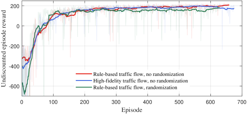
Figure 4: Undiscounted episode reward during training under three traffic flows. The three differently colored solid lines represent the training curves of the same reinforcement learning algorithm under different microscopic traffic flows.

Table 7: The results of testing three trained policies under three traffic flows in freeway.

		Training
			$\mathbf{no\,randomization}$	$\mathbf{fidelity}$	$\mathbf{randomization}$
Testing	$\mathbf{no\,randomization}$	Average reward	200.50	205.32	197.15
		Success rate	100%	99.70%	100%
	$\mathbf{fidelity}$	Average reward	187.10	208.85	202.48
		Success rate	98.90%	99.60%	99.90%
	$\mathbf{randomization}$	Average reward	126.27	160.06	186.72
		Success rate	80.40%	89.00%	99.40%

The results of testing are shown in Table 7, it can be observed that the policy trained under domain randomization microscopic traffic flows has the highest success rate and close to $100\%$ when tested under different microscopic traffic flows, and its rewards are relatively stable.The policy trained under microscopic traffic flow without randomization and high-fidelity microscopic traffic flow cannot adapt to complex traffic flow environments, and the success rate and reward of the tests in domain randomization microscopic traffic flow are relatively low.

4.2.4 Test Results for Increasing Traffic Density

Due to the heightened interactivity among vehicles in freeway scene, the traffic density significantly affects the ego vehicle. The impact of changes in traffic density is shown in Table 8, it can be observed that the success rate and reward of the policy trained under microscopic traffic flow without randomization decreases significantly as traffic density increases. In contrast, the policy trained under domain randomization microscopic traffic flow maintains a success rate near $100\%$, with both success rate and rewards remaining stable.

Table 8: The impact of changes in traffic density on three trained policies under the high-fidelity microscopic traffic flow.

		Traffic density for testing under high-fidelity traffic flow
			$\boldsymbol{\phi_{h}=0.14}$	$\boldsymbol{\phi_{h}=0.18}$	$\boldsymbol{\phi_{h}=0.20}$
Training with  rule-based traffic flow $(\boldsymbol{\phi=0.14})$	$\mathbf{no\,randomization}$	Average speed	16.39	15.89	15.77
		Average reward	187.10	189.85	109.49
		Success rate	98.90%	93.90%	66.50%
	$\mathbf{randomization}$	Average speed	15.83	15.42	15.17
		Average reward	202.48	197.48	191.51
		Success rate	99.90%	99.80%	99.90%

* $\phi_{h}$ is the vehicle generation probability of high-fidelity microscopic traffic flow, defined as the number of vehicles that are generated from the starting point per second. $\phi$ is the vehicle generation probability of certain microscopic traffic flow.

5 Conclusion

In this study, we introduce a method for randomizing lane-changing and car-following model parameters to generate microscopic traffic flows, and we evaluate and compare the policies trained by reinforcement learning algorithms in the freeway and merging environments under different microscopic traffic flows. The results show that:

• Policy trained under the domain randomization microscopic traffic flow is able to maintain high rewards and success rates when tested under different microscopic traffic flows. However, the policy trained under microscopic traffic flow without randomization or high-fidelity micro traffic flow perform significantly worse when tested under different microscopic traffic flows. It indicates that domain randomization traffic flow has excellent adaptability to different types of traffic flow types.
  

• Policy trained under the domain randomized rule-based microscopic traffic flow perform well when tested under high-fidelity microscopic traffic flow with different traffic densities. The policy trained under microscopic traffic flow without randomization decreases significantly with increasing traffic density. It indicates that the domain randomized traffic flow possesses strong adaptability to changes in traffic density.
  

• Although high-fidelity microscopic traffic flow is close to real microscopic traffic flows, the results show that not only does it considerably increase simulation time, but policies trained in this microscopic traffic flow also do not perform very well with different microscopic flows. Therefore, high-fidelity microscopic traffic flow is more suitable for testing rather than training.
  

In summary, policies trained under domain randomized rule-based microscopic traffic flow demonstrate robust performance when transferred to environments that closely resemble real-world traffic conditions. Future work includes testing the policy trained under the domain randomized rule-based microscopic traffic flow on a real autonomous vehicle.

Conceptualization, Y.L.; methodology, A.X., Y.L., and X.L.; formal analysis, A.X. and Y.L.; investigation, A.X. and Y.L.; data curation, A.X.; writing—original draft preparation, A.X.; writing—review and editing, A.X.; supervision, Y.L.; All authors have read and agreed to the published version of the manuscript.

Not applicable.

Not applicable.

Not applicable.

The data can be obtained upon reasonable request from the corresponding author.

The authors declare that they have no known competing financial interest or personal relationships that could have appeared to influence the work reported in this paper.

References

References

- Le Vine et al. (2015) Le Vine, S.; Zolfaghari, A.; Polak, J. Autonomous cars: The tension between occupant experience and intersection capacity. Transportation Research Part C: Emerging Technologies 2015, 52, 1–14.
- Sallab et al. (2017) Sallab, A.E.; Abdou, M.; Perot, E.; Yogamani, S. Deep reinforcement learning framework for autonomous driving. arXiv preprint arXiv:1704.02532 2017.
- Hoel et al. (2018) Hoel, C.J.; Wolff, K.; Laine, L. Automated speed and lane change decision making using deep reinforcement learning. In Proceedings of the 2018 21st International Conference on Intelligent Transportation Systems (ITSC). IEEE, 2018, pp. 2148–2155.
- Ye et al. (2019) Ye, Y.; Zhang, X.; Sun, J. Automated vehicle’s behavior decision making using deep reinforcement learning and high-fidelity simulation environment. Transportation Research Part C: Emerging Technologies 2019, 107, 155–170.
- Ye et al. (2020) Ye, F.; Cheng, X.; Wang, P.; Chan, C.Y.; Zhang, J. Automated lane change strategy using proximal policy optimization-based deep reinforcement learning. In Proceedings of the 2020 IEEE Intelligent Vehicles Symposium (IV). IEEE, 2020, pp. 1746–1752.
- Lin et al. (2020) Lin, Y.; McPhee, J.; Azad, N.L. Anti-jerk on-ramp merging using deep reinforcement learning. In Proceedings of the 2020 IEEE Intelligent Vehicles Symposium (IV). IEEE, 2020, pp. 7–14.
- Peng et al. (2022) Peng, J.; Zhang, S.; Zhou, Y.; Li, Z. An Integrated Model for Autonomous Speed and Lane Change Decision-Making Based on Deep Reinforcement Learning. IEEE Transactions on Intelligent Transportation Systems 2022, 23, 21848–21860.
- Mirchevska et al. (2017) Mirchevska, B.; Blum, M.; Louis, L.; Boedecker, J.; Werling, M. Reinforcement learning for autonomous maneuvering in highway scenarios. In Proceedings of the Workshop for Driving Assistance Systems and Autonomous Driving, 2017, pp. 32–41.
- Treiber et al. (2000) Treiber, M.; Hennecke, A.; Helbing, D. Congested traffic states in empirical observations and microscopic simulations. Physical review E 2000, 62, 1805.
- Liu et al. (2021) Liu, J.; Zeng, W.; Urtasun, R.; Yumer, E. Deep structured reactive planning. In Proceedings of the 2021 IEEE International Conference on Robotics and Automation (ICRA). IEEE, 2021, pp. 4897–4904.
- Huang et al. (2022) Huang, X.; Rosman, G.; Jasour, A.; McGill, S.G.; Leonard, J.J.; Williams, B.C. TIP: Task-informed motion prediction for intelligent vehicles. In Proceedings of the 2022 IEEE/RSJ International Conference on Intelligent Robots and Systems (IROS). IEEE, 2022, pp. 11432–11439.
- Punzo and Simonelli (2005) Punzo, V.; Simonelli, F. Analysis and comparison of microscopic traffic flow models with real traffic microscopic data. Transportation Research Record 2005, 1934, 53–63.
- Tessler et al. (2019) Tessler, C.; Efroni, Y.; Mannor, S. Action robust reinforcement learning and applications in continuous control. In Proceedings of the International Conference on Machine Learning. PMLR, 2019, pp. 6215–6224.
- Wang et al. (2016) Wang, J.X.; Kurth-Nelson, Z.; Tirumala, D.; Soyer, H.; Leibo, J.Z.; Munos, R.; Blundell, C.; Kumaran, D.; Botvinick, M. Learning to reinforcement learn. arXiv preprint arXiv:1611.05763 2016.
- Andrychowicz et al. (2020) Andrychowicz, O.M.; Baker, B.; Chociej, M.; Jozefowicz, R.; McGrew, B.; Pachocki, J.; Petron, A.; Plappert, M.; Powell, G.; Ray, A.; et al. Learning dexterous in-hand manipulation. The International Journal of Robotics Research 2020, 39, 3–20.
- Sheckells et al. (2019) Sheckells, M.; Garimella, G.; Mishra, S.; Kobilarov, M. Using data-driven domain randomization to transfer robust control policies to mobile robots. In Proceedings of the 2019 International Conference on Robotics and Automation (ICRA). IEEE, 2019, pp. 3224–3230.
- Wenl et al. (2023) Wenl, L.; Fu, D.; Mao, S.; Cai, P.; Dou, M.; Li, Y.; Qiao, Y. LimSim: A long-term interactive multi-scenario traffic simulator. In Proceedings of the 2023 IEEE 26th International Conference on Intelligent Transportation Systems (ITSC). IEEE, 2023, pp. 1255–1262.
- Fellendorf and Vortisch (2010) Fellendorf, M.; Vortisch, P. Microscopic traffic flow simulator VISSIM. Fundamentals of traffic simulation 2010, pp. 63–93.
- Casas et al. (2010) Casas, J.; Ferrer, J.L.; Garcia, D.; Perarnau, J.; Torday, A. Traffic simulation with aimsun. Fundamentals of traffic simulation 2010, pp. 173–232.
- Lopez et al. (2018) Lopez, P.A.; Behrisch, M.; Bieker-Walz, L.; Erdmann, J.; Flötteröd, Y.P.; Hilbrich, R.; Lücken, L.; Rummel, J.; Wagner, P.; Wießner, E. Microscopic traffic simulation using sumo. In Proceedings of the 2018 21st international conference on intelligent transportation systems (ITSC). IEEE, 2018, pp. 2575–2582.
- Shah et al. (2018) Shah, S.; Dey, D.; Lovett, C.; Kapoor, A. Airsim: High-fidelity visual and physical simulation for autonomous vehicles. In Proceedings of the Field and Service Robotics: Results of the 11th International Conference. Springer, 2018, pp. 621–635.
- Dosovitskiy et al. (2017) Dosovitskiy, A.; Ros, G.; Codevilla, F.; Lopez, A.; Koltun, V. CARLA: An open urban driving simulator. In Proceedings of the Conference on robot learning. PMLR, 2017, pp. 1–16.
- Li et al. (2022) Li, Q.; Peng, Z.; Feng, L.; Zhang, Q.; Xue, Z.; Zhou, B. Metadrive: Composing diverse driving scenarios for generalizable reinforcement learning. IEEE transactions on pattern analysis and machine intelligence 2022, 45, 3461–3475.
- Sun et al. (2022) Sun, Q.; Huang, X.; Williams, B.C.; Zhao, H. InterSim: Interactive traffic simulation via explicit relation modeling. In Proceedings of the 2022 IEEE/RSJ International Conference on Intelligent Robots and Systems (IROS). IEEE, 2022, pp. 11416–11423.
- Feng et al. (2023) Feng, L.; Li, Q.; Peng, Z.; Tan, S.; Zhou, B. Trafficgen: Learning to generate diverse and realistic traffic scenarios. In Proceedings of the 2023 IEEE International Conference on Robotics and Automation (ICRA). IEEE, 2023, pp. 3567–3575.
- Zheng et al. (2022) Zheng, O.; Abdel-Aty, M.; Yue, L.; Abdelraouf, A.; Wang, Z.; Mahmoud, N. CitySim: A drone-based vehicle trajectory dataset for safety oriented research and digital twins. arXiv preprint arXiv:2208.11036 2022.
- Low et al. (2019) Low, E.S.; Ong, P.; Cheah, K.C. Solving the optimal path planning of a mobile robot using improved Q-learning. Robotics and Autonomous Systems 2019, 115, 143–161.
- Cailhol et al. (2019) Cailhol, S.; Fillatreau, P.; Zhao, Y.; Fourquet, J.Y. Multi-layer path planning control for the simulation of manipulation tasks: Involving semantics and topology. Robotics and Computer-Integrated Manufacturing 2019, 57, 17–28.
- Berrazouane et al. (2019) Berrazouane, M.; Tong, K.; Solmaz, S.; Kiers, M.; Erhart, J. Analysis and initial observations on varying penetration rates of automated vehicles in mixed traffic flow utilizing sumo. In Proceedings of the 2019 IEEE International Conference on Connected Vehicles and Expo (ICCVE). IEEE, 2019, pp. 1–7.
- Krajzewicz et al. (2012) Krajzewicz, D.; Erdmann, J.; Behrisch, M.; Bieker, L. Recent development and applications of SUMO-Simulation of Urban MObility. International journal on advances in systems and measurements 2012, 5.
- Wegener et al. (2008) Wegener, A.; Piórkowski, M.; Raya, M.; Hellbrück, H.; Fischer, S.; Hubaux, J.P. TraCI: an interface for coupling road traffic and network simulators. In Proceedings of the Proceedings of the 11th communications and networking simulation symposium, 2008, pp. 155–163.
- Haarnoja et al. (2018) Haarnoja, T.; Zhou, A.; Hartikainen, K.; Tucker, G.; Ha, S.; Tan, J.; Kumar, V.; Zhu, H.; Gupta, A.; Abbeel, P.; et al. Soft actor-critic algorithms and applications. arXiv preprint arXiv:1812.05905 2018.
- Lin et al. (2024) Lin, Y.; Liu, X.; Zheng, Z.; Wang, L. Discretionary Lane-Change Decision and Control via Parameterized Soft Actor-Critic for Hybrid Action Space. arXiv preprint arXiv:2402.15790 2024.
- Hausknecht and Stone (2015) Hausknecht, M.; Stone, P. Deep reinforcement learning in parameterized action space. arXiv preprint arXiv:1511.04143 2015.