Efficient sparse probability measures recovery via Bregman gradient

Abstract

This paper presents an algorithm tailored for the efficient recovery of sparse probability measures incorporating $\ell_{0}$-sparse regularization within the probability simplex constraint. Employing the Bregman proximal gradient method, our algorithm achieves sparsity by explicitly solving underlying subproblems. We rigorously establish the convergence properties of the algorithm, showcasing its capacity to converge to a local minimum with a convergence rate of $O(1/k)$ under mild assumptions. To substantiate the efficacy of our algorithm, we conduct numerical experiments, offering a compelling demonstration of its efficiency in recovering sparse probability measures.
Keywords $\ell_{0}$-sparse regularization, Probability simplex constraint, Bregman proximal gradient

1 Introduction

In this paper, we focus on solving the following sparse optimization problem with the $\ell_{0}$ regularization and the probability simplex constraint:

$$\min_{\boldsymbol{x}\in\mathbb{R}^{n}} f(\boldsymbol{x})+\lambda\|\boldsymbol{x}\|_{0}$$ (1.1)

subject to $$\mathbf{1}^{\top}\boldsymbol{x}=1,\boldsymbol{x}\geq 0,$$

where $f:\mathbb{R}^{n}\rightarrow(-\infty,\infty]$ is proper, continuously differentiable and convex, $\lambda>0$ is a regularization parameter, $\mathbf{1}\in\mathbb{R}^{n}$ is the vector with all ones, and $\boldsymbol{x}\geq 0$ indicates that all elements in $\boldsymbol{x}$ are nonnegative. The $\ell_{0}$ “norm” of a vector $\boldsymbol{x}$ counts the number of nonzero elements in $\boldsymbol{x}$. This problem encompasses various applications, including sparse portfolio optimization [6, 32, 13] and sparse hyperspectral unmixing [27, 28, 15].

Various approaches are available for solving optimization problems with the $\ell_{0}$ term. The iterative hard-thresholding (IHT) algorithm was proposed for $\ell_{0}$-regularized least squares problems [8, 9]. When the simplex constraint is incorporated, the paper [33] proposed an algorithm based on IHT and established its convergence properties to learn sparse probability measures. However, algorithms based on IHT require strong assumptions, such as mutual coherence [17] and restricted isometry condition [9].

Due to the NP-hard nature of the $\ell_{0}$ term [24], computationally feasible methods based on the $\ell_{1}$ norm, e.g., Lasso [29], have been introduced for problems without the simplex constraint. However, this relaxation does not work for the simplex constraint because the $\ell_{1}$ norm remains a constant for all feasible solutions.

Other alternative terms were used besides the $\ell_{0}$ and $\ell_{1}$ terms. E.g., an iteratively reweighted algorithm based on the logarithm smoothed function was proposed in [28]. The paper [15] presented an alternating direction method of multipliers (ADMM) algorithm to solve the following problem:

$$\min_{\boldsymbol{x}\in\mathbb{R}^{n}}\frac{1}{2}\|\mathbf{A}\boldsymbol{x}-\boldsymbol{b}\|^{2}+\lambda F(\sigma,\boldsymbol{x})\quad\text{ subject to }\mathbf{1}^{\top}\boldsymbol{x}=1,~{}\boldsymbol{x}\geq 0,$$ (1.2)

where $\mathbf{A}\in\mathbb{R}^{m\times n},~{}\boldsymbol{b}\in\mathbb{R}^{m}$, $\lambda>0$ is a regularized parameter, and $F(\sigma,\boldsymbol{x})=g(\sigma)\sum\limits_{i=1}^{n}\arctan(\sigma x_{i})$ with $\sigma>0$. The function $g(\sigma)$ is chosen such that $F(\sigma,\boldsymbol{x})$ tends to $\|\boldsymbol{x}\|_{0}$ as $\sigma\rightarrow\infty$. The paper [30] used the $\ell_{1/2}$ norm regularization and solves the following equivalent problem:

$$\min_{\boldsymbol{y}\in\mathbb{R}^{n}}\frac{1}{2}\|\mathbf{A}(\boldsymbol{y}\odot\boldsymbol{y})-\boldsymbol{b}\|_{2}^{2}+\lambda\|\boldsymbol{y}\|_{1}\quad\text{subject to }\boldsymbol{y}^{\top}\boldsymbol{y}=1,$$ (1.3)

where $\lambda>0$ is a regularized parameter and the symbol ‘$\odot$’ means the Hadamard product of two vectors. This paper introduced a geometric proximal gradient (GPG) method to solve the above problem.

Although approximation models offer computational advantages, they may not precisely capture the solution of the original $\ell_{0}$-based model [34]. Notably, an increasing body of research based on the $\ell_{0}$ term has recently emerged and attracted significant attention due to their remarkable recovery properties. In this context, noteworthy contributions have been made, such as normalized IHT and improved IHT [10, 26]. Furthermore, to expedite convergence rates, various second-order algorithms rooted in the $\ell_{0}$ term, incorporating Newton-type steps, have been proposed [34, 35, 36]. Despite the NP-hardness of the problem, the utilization of the $\ell_{0}$ term still has gained prominence in the realm of selecting sparse features.

This paper employs the Bregman proximal gradient (BPG) method to solve (1.1) and provides its theoretical guarantee. One of the primary challenges in solving (1.1) lies in projecting the solution onto the probabilistic simplex set. To tackle this challenge, we leverage BPG, allowing fast iterations by designing a suitable Bregman divergence (such as relative entropy, detailed in Section 2.1 or Itakura-Saito distance). This choice mitigates computational burdens and reduces per-iteration complexity, facilitating effective convergence. Instead of enforcing a fixed number of elements to be zero, as done in methods like IHT [8, 9], we add a $\ell_{0}$ term and give an explicit expression of the global solution of the subproblem in each BPG iteration. The number of nonzero elements in each iteration adjusts according to the current iteration and the regularization parameter, providing greater flexibility than methods with a fixed number of nonzero elements. We establish the global convergence of our proposed algorithm and prove that the generated sequence converges to a local minimizer with the rate $O(1/k)$. Furthermore, while prior research predominantly relied on smoothed $\ell_{0}$ term [30], our numerical results demonstrate that our proposed algorithm can achieve more accurate outcomes within a shorter timeframe.

Notation. Through this paper, we use bold lower letters for vectors, bold capital letters for matrices, and regular lower letters for scalars. The regular letter with a subscript indicates the corresponding element of the vector, e.g., $x_{1}$ is the first element of the vector $\boldsymbol{x}$. Let $\mathbb{R}^{m\times n}$ be the set of all $m\times n$ real matrices and $\mathbb{R}^{n}$ be equipped with the Euclidean inner product $\langle\cdot\rangle$. The symbol ‘$\odot$’ represents the Hadamard product of two vectors. We denote $\|\cdot\|_{p}$ as the $\ell_{p}$ norm of a vector. For simplicity, we use $\|\cdot\|$ to denote the Euclidean norm. For any $\boldsymbol{x}=(x_{1},x_{2},...,x_{n})^{\top}\in\mathbb{R}^{n}$ and any set $I$, let $|I|$ denote the number of the elements in the set $I$ and $\text{supp}(\boldsymbol{x}):=\{i\in[n]:x_{i}\neq 0\}$, where $[n]:=\{1,2,...,n\}$.

2 The Proposed Algorithm

We first introduce the standard BPG in Subsection 2.1. When applying BPG to our problem (1.1) in Section 2.2, we must solve a subproblem with the $\ell_{0}$ term. Then, we propose a method to solve the subproblem analytically in Subsection 2.3. We show that our BPG algorithm for solving the problem (1.1) converges in a finite number of iterations in Subsection 2.4.

2.1 Introduction to the Bregman proximal gradient

The Bregman proximal gradient (BPG) method, also known as mirror descent (MD) [2, 14, 11, 5, 3, 25], solves the following optimization problem

$$\min_{\boldsymbol{x}\in C}\ f(\boldsymbol{x}),$$ (2.1)

where $C$ is a closed convex set and the objective function $f$ is proper and continuously differentiable.

Let $h$ be a strictly convex function that is differentiable on an open set containing the relative interior of $C$ [12], which is denoted as $\mbox{rint}(C)$. For $\boldsymbol{y}\in\mbox{rint}(C)$, the Bregman divergence generated by $h$ is defined as

$$D_{h}(\boldsymbol{x},\boldsymbol{y})=h(\boldsymbol{x})-h(\boldsymbol{y})-\langle\nabla h(\boldsymbol{y}),\boldsymbol{x}-\boldsymbol{y}\rangle,$$ (2.2)

where $\boldsymbol{x}\in\text{dom}(h)$.

Definition 1.

The function $f$ is called $L$-smooth relative to $h$ on $C$ if there exists $L>0$ such that, for $\boldsymbol{x}\in C$ and $\boldsymbol{y}\in\mbox{rint}(C)$,

$$f(\boldsymbol{x})\leq f(\boldsymbol{y})+\langle\nabla f(\boldsymbol{y}),\boldsymbol{x}-\boldsymbol{y}\rangle+LD_{h}(\boldsymbol{x},\boldsymbol{y}).$$ (2.3)

The definition of relative smoothness provides an upper bound for $f(\boldsymbol{x})$. If $f$ is $L$-smooth relative to $h$ on $C$, BPG updates the estimate of $\boldsymbol{x}$ via solving the following problems:

$$\boldsymbol{x}^{k+1}\in\arg\min_{\boldsymbol{x}\in C}\left(f(\boldsymbol{x}^{k})+\langle\nabla f(\boldsymbol{x}^{k}),\boldsymbol{x}-\boldsymbol{x}^{k}\rangle+\frac{1}{\alpha}D_{h}(\boldsymbol{x},\boldsymbol{x}^{k})\right),$$ (2.4)

where $0<\alpha<1/L$.

The Bregman divergence generated by $h(\boldsymbol{x})=\frac{1}{2}\|\boldsymbol{x}\|^{2}$ is the squared Euclidean distance $D_{h}(\boldsymbol{x},\boldsymbol{y})=\frac{1}{2}\|\boldsymbol{x}-\boldsymbol{y}\|^{2}$, and the corresponding algorithm is the standard proximal gradient algorithm. A proper Bregman divergence can exploit optimization problems’ structure [3] and reduce the per-iteration complexity. BPG has demonstrated numerous advantages in terms of computational efficiency in solving constrained optimization problems [2, 1, 21, 5, 22, 20, 19].

One of the most intriguing examples occurs when $C$ represents the probabilistic simplex set [5]. In this context, the proximal map becomes straightforward to compute when we utilize $h(\boldsymbol{x})=\sum_{i=1}^{n}x_{i}\log x_{i}$ with the convention $0\log 0=0$ to generate the Bregman divergence. The Bregman divergence associated with such $h$ is

$$D_{h}(\boldsymbol{x},\boldsymbol{y})=\sum_{i=1}^{n}\left(x_{i}\log\left(\frac{x_{i}}{y_{i}}\right)-x_{i}+y_{i}\right),$$ (2.5)

which is also known as KL-divergence or relative entropy. Under the simplex set constraint, the update (2.4) admits the closed-form solution:

$$x_{i}^{k+1}=\frac{x_{i}^{k}e^{-\alpha\nabla_{x_{i}}f(\boldsymbol{x}^{k})}}{\sum_{j=1}^{n}x_{j}^{k}e^{-\alpha\nabla_{x_{j}}f(\boldsymbol{x}^{k})}}\quad\forall\ i=1,2,...,n.$$ (2.6)

The update of $\boldsymbol{x}^{k+1}$ in (2.6) is much faster than the projection to the simplex set in the standard projected gradient descent.

When $f$ is convex, BPG has a $O(1/k)$ convergence rate [2, 7, 21]. The paper [18] proposed an accelerated Bregman proximal gradient method (ABPG) and ABPG with gain adaptation (ABPG-g), which have a faster convergence rate than BPG. Algorithm 1 presents the ABPG-g algorithm. According to [18], when applied under the probabilistic simplex set constraint with KL-divergence as the Bregman divergence and worked with intrinsic triangle scaling exponent $\gamma=2$ [18, Definition 3], ABPG-g demonstrates an empirical convergence rate of $O(1/k^{2})$.

Algorithm 1 ABPG with gain adaptation (ABPG-g)

0:  $\boldsymbol{z}^{0}=\boldsymbol{x}^{0}\in C,\ \gamma>1,\ \rho>1,\ \theta_{0}=1,\ G_{-1}=1$, $G_{\text{min}}>0$, $k=0$, and $\varepsilon_{1}>0$.

  repeat

     $G_{k}=\max\{G_{k-1}/\rho,G_{\text{min}}\}$

     repeat

        if $k>0$ then

           compute $\theta_{k}$ by solving $\frac{1-\theta_{k}}{G_{k}\theta_{k}^{\gamma}}=\frac{1}{G_{k-1}\theta_{k-1}^{\gamma}}$.

        end if

        $\boldsymbol{y}^{k}=(1-\theta_{k})\boldsymbol{x}^{k}+\theta_{k}\boldsymbol{z}^{k}$

        $\boldsymbol{z}^{k+1}=\arg\min\limits_{\boldsymbol{z}\in C}\left\{f(\boldsymbol{y}^{k})+\langle\nabla f(\boldsymbol{y}^{k}),\boldsymbol{z}-\boldsymbol{y}^{k}\rangle+G_{k}\theta_{k}^{\gamma-1}LD_{h}(\boldsymbol{z},\boldsymbol{z}^{k})\right\}$

        $\boldsymbol{x}^{k+1}=(1-\theta_{k})\boldsymbol{x}^{k}+\theta_{k}\boldsymbol{z}^{k+1}$

        $G_{k}\mapsfrom G_{k}\rho$

     until $f(\boldsymbol{x}^{k+1})\leq f(\boldsymbol{y}^{k})+\langle\nabla f(\boldsymbol{y}^{k}),\boldsymbol{x}^{k+1}-\boldsymbol{y}^{k}\rangle+G_{k}\theta_{k}^{\gamma}LD_{h}(\boldsymbol{z}^{k+1},\boldsymbol{z}^{k})$

     $k\mapsfrom k+1$

  until $|f(\boldsymbol{x}^{k+1})-f(\boldsymbol{x}^{k})|<\varepsilon_{1}$

2.2 Applying BPG to problem (1.1)

To begin with, it is important to emphasize that the iterates (2.6) generated by BPG never reside on the boundary, i.e., ${x}^{k}_{i}\neq 0$ as long as the initial ${x}^{0}_{i}\neq 0$ for any index $i\in[n]$. However, these iterates may converge to the boundary without a sparse penalty term. We let the $\ell_{0}$ term be the penalty term to achieve sparsity during the iteration. Extensive research has demonstrated the effectiveness of the $\ell_{0}$ term in driving the iterates towards sparse solutions. Notably, the $\ell_{0}$ term exhibits stronger sparsity characteristics than alternative terms [31], motivating us to employ it. In conclusion, by incorporating the $\ell_{0}$ term into the BPG algorithm, we aim to solve the following subproblem:

$$\boldsymbol{x}^{k+1}\in\arg\min_{\mathbf{1}^{\top}\boldsymbol{x}=1}\left(f(\boldsymbol{x}^{k})+\langle\nabla f(\boldsymbol{x}^{k}),\boldsymbol{x}-\boldsymbol{x}^{k}\rangle+\frac{1}{\alpha}D_{h}(\boldsymbol{x},\boldsymbol{x}^{k})+\lambda\|\boldsymbol{x}\|_{0}\right),$$

where $\boldsymbol{x}^{k}$ is the current iterate, $D_{h}(\boldsymbol{x},\boldsymbol{x}^{k})$ is the KL-divergence between $\boldsymbol{x}$ and $\boldsymbol{x}^{k}$, $\alpha>0$ and $\lambda>0$ are two constants.

Based on the above analysis, our algorithm for solving problem (1.1) can be described as follows in Algorithm 2.

Algorithm 2 Our proposed algorithm for (1.1)

0:  $\lambda,\varepsilon_{2}$, $\alpha>0$, $k=0$.

  (Initialization): Use ABPG-g (Algorithm 1) to attain $\boldsymbol{x}^{0}$ (note: $\|\boldsymbol{x}^{0}\|_{0}=n$).

  repeat

     (L0BPG): Update $\boldsymbol{x}^{k+1}$ via

$$\boldsymbol{x}^{k+1}\in\arg\min_{\mathbf{1}^{\top}\boldsymbol{x}=1}\left(f(\boldsymbol{x}^{k})+\langle\nabla f(\boldsymbol{x}^{k}),\boldsymbol{x}-\boldsymbol{x}^{k}\rangle+\frac{1}{\alpha}D_{h}(\boldsymbol{x},\boldsymbol{x}^{k})+\lambda\|\boldsymbol{x}\|_{0}\right).$$ (2.7)

     $k\mapsfrom k+1$

  until $f(\boldsymbol{x}^{k})+\lambda\|\boldsymbol{x}^{k}\|_{0}-f(\boldsymbol{x}^{k+1})-\lambda\|\boldsymbol{x}^{k+1}\|_{0}<\varepsilon_{2}$

Remark 2.1.

At the initialization phase of Algorithm 2, we utilize ABPG-g to obtain a proper starting point $\boldsymbol{x}^{0}$. As demonstrated in [18], ABPG-g exhibits an empirical convergence rate of $O(1/k^{2})$, which is notably faster than the convergence rate of $O(k^{-1})$ observed in BPG [7, 2]. Consequently, we can establish an appropriate starting point via ABPG-g more expeditiously than BPG. Furthermore, it’s important to note that we do not achieve a sparse solution during this initialization phase, i.e., $\|\boldsymbol{x}^{0}\|_{0}=n$.

2.3 Analytical solution to the subproblem (2.7)

The following theorem provides a way to find a global solution to the subproblem (2.7).

Theorem 1.

Let

$$\boldsymbol{y}^{k+1}=\arg\min_{\mathbf{1}^{\top}\boldsymbol{x}=1}\left(f(\boldsymbol{x}^{k})+\langle\nabla f(\boldsymbol{x}^{k}),\boldsymbol{x}-\boldsymbol{x}^{k}\rangle+\frac{1}{\alpha}D_{h}(\boldsymbol{x},\boldsymbol{x}^{k})\right)$$ (2.8)

and

$$d\in\arg\min_{m\in[n]}-\frac{1}{\alpha}\log\sum_{i=1}^{m}y^{k+1}_{(i)}+\lambda m,$$

where $y^{k+1}_{(i)}$ represents the $i$-th largest element of $\boldsymbol{y}^{k+1}$,i.e. $y^{k+1}_{(1)}\geq y^{k+1}_{(2)}\geq...\geq y^{k+1}_{(n)}$, then we obtain a global solution to the subproblem (2.7) as

$$x_{i}^{k+1}=\left\{\begin{aligned} &\frac{y^{k+1}_{i}}{\sum_{j\in I_{k+1}}y^{k+1}_{j}},&\quad\mbox{if }i\in I_{k+1},\\ &0,&\quad otherwise,\end{aligned}\right.$$ (2.9)

where $I_{k+1}$ is the set of the indices of the first $d$ largest entries of $\boldsymbol{y}^{k+1}$.

Proof.

Denote $g(x_{i})=x_{i}\nabla_{x_{i}}f(\boldsymbol{x}^{k})+\frac{x_{i}}{\alpha}\log\left(\frac{x_{i}}{x_{i}^{k}}\right)$. Then the subproblem (2.7) can be rewritten as

$$\min_{\mathbf{1}^{\top}\boldsymbol{x}=1}f(\boldsymbol{x}^{k})+\langle\nabla f(\boldsymbol{x}^{k}),\boldsymbol{x}-\boldsymbol{x}^{k}\rangle+\frac{1}{\alpha}D_{h}(\boldsymbol{x},\boldsymbol{x}^{k})+\lambda\|\boldsymbol{x}\|_{0}$$ (2.10)

$$= \min_{\mathbf{1}^{\top}\boldsymbol{x}=1}\sum_{i=1}^{n}g(x_{i})+\lambda\|\boldsymbol{x}\|_{0}+c$$

$$= \min_{m\in[n]}\ \min_{\mathbf{1}^{\top}\boldsymbol{x}=1,\|\boldsymbol{x}\|_{0}=m}\sum_{i=1}^{n}g(x_{i})+\lambda m+c$$

$$= \min_{m\in[n]}\ \min_{\mathbf{1}^{\top}\boldsymbol{x}=1,\|\boldsymbol{x}\|_{0}=m}\sum_{i\in\text{supp}(\boldsymbol{x})}g(x_{i})+\lambda m+c,$$

where $c=f(\boldsymbol{x}^{k})-\langle\nabla f(\boldsymbol{x}^{k}),\boldsymbol{x}^{k}\rangle$. The last equality holds since $g(0)=0$.

Let’s consider the inner minimization problem first

$$\min_{\mathbf{1}^{\top}\boldsymbol{x}=1,\|\boldsymbol{x}\|_{0}=m}\sum_{i\in\text{supp}(\boldsymbol{x})}g(x_{i})=\min_{|I|=m}\quad\min_{\mathbf{1}^{\top}\boldsymbol{x}=1,~{}\text{supp}(\boldsymbol{x})=I}\sum_{i\in I}g(x_{i}).$$ (2.11)

There are $C_{n}^{m}$ possible ways to choose the support $I$ of $m$ elements from the $n$ elements. For each fixed support of $m$ elements, we can find the optimal $\boldsymbol{x}$ analytically. Then, the problem becomes finding the support of $m$ elements with the smallest function value from those possible ways. Given the support $I$ of $m$ elements for $\boldsymbol{x}$, we can solve the problem analytically as below:

$$x_{m,i}^{k+1}=\left\{\begin{aligned} &\frac{x_{i}^{k}e^{-\alpha\nabla_{x_{i}}f(\boldsymbol{x}^{k})}}{\sum_{j\in I}x_{j}^{k}e^{-\alpha\nabla_{x_{j}}f(\boldsymbol{x}^{k})}},&\quad\mbox{if }i\in I,\\ &0,&\quad\mbox{otherwise.}\end{aligned}\right.$$ (2.12)

We plug this solution into the objective function in (2.11) and obtain

$$\sum_{i\in I}g(x_{m,i}^{k+1})=-\frac{1}{\alpha}\log\sum_{i\in I}x_{i}^{k}e^{-\alpha\nabla_{x_{i}}f(\boldsymbol{x}^{k})}.$$

Note that the optimization problem in (2.8) gives that

$${y}_{i}^{k+1}=\frac{{x_{i}}^{k}e^{-\alpha\nabla_{x_{i}}f(\boldsymbol{x}^{k})}}{\sum_{j=1}^{n}{x}^{k}_{j}e^{-\alpha\nabla_{x_{j}}f(\boldsymbol{x}^{k})}}.$$

Therefore, the objective function in (2.11) becomes

$$\sum_{i\in I}g(x_{m,i}^{k+1})=-\frac{1}{\alpha}\log\sum_{i\in I}y_{i}^{k+1}-\frac{1}{\alpha}\log\sum_{j=1}^{n}{x}^{k}_{j}e^{-\alpha\nabla_{x_{j}}f(\boldsymbol{x}^{k})}.$$

Thus, we must choose the indices for the $m$ largest elements from $\boldsymbol{y}^{k+1}$.

Since the inner optimization problem in (2.10) can be solved analytically, the subproblem (2.7) reduces to finding the number $m$ by solving the problem

$$\min_{m\in[n]}\ -\frac{1}{\alpha}\log\sum_{i=1}^{m}{y}^{k+1}_{(i)}+\lambda m-\frac{1}{\alpha}\log\sum_{j=1}^{n}{x}^{k}_{j}e^{-\alpha\nabla_{x_{j}}f(\boldsymbol{x}^{k})}+c,$$ (2.13)

which is equivalent to

$$d\in\arg\min_{m\in[n]}-\frac{1}{\alpha}\log\sum_{i=1}^{m}{y}^{k+1}_{(i)}+\lambda m.$$

After we find the number $d$, we choose the indices as the largest $d$ elements from $\boldsymbol{y}^{k+1}$, then we construct $\boldsymbol{x}^{k+1}$ based on the equation (2.9). ∎

Based on Theorem 1, we can solve the problem (2.7) by Algorithm 3. Given that there may be two choices for $d$, we opt to select the larger one, i.e.,

$$d_{k+1}:=\max\left\{\arg\min_{m\in[n]}-\frac{1}{\alpha}\log\sum_{i=1}^{m}{y}^{k+1}_{(i)}+\lambda m\right\}.$$ (2.14)

Algorithm 3 Algorithm to solve the problem (2.7)

  (BPG step): Update $\boldsymbol{y}^{k+1}$ via

$$\boldsymbol{y}^{k+1}=\arg\min_{\mathbf{1}^{\top}\boldsymbol{y}=1}\left(f(\boldsymbol{x}^{k})+\langle\nabla f(\boldsymbol{x}^{k}),\boldsymbol{y}-\boldsymbol{x}^{k}\rangle+\frac{1}{\alpha}D_{h}(\boldsymbol{y},\boldsymbol{x}^{k})\right).$$ (2.15)

  (Sorting step): Find $d_{k+1}$ such that

$$d_{k+1}=\max\left\{\arg\min_{m\in[n]}-\frac{1}{\alpha}\log\sum_{i=1}^{m}{y}^{k+1}_{(i)}+\lambda m\right\},$$ (2.16)

where we order the elements of $\boldsymbol{y}^{k+1}:y_{(1)}^{k+1}\geq y_{(2)}^{k+1}\geq...\geq y_{(n)}^{k+1}$.

  (Removing step): Update $\boldsymbol{x}^{k+1}$ by

$$x_{i}^{k+1}=\left\{\begin{aligned} &\frac{y^{k+1}_{i}}{\sum_{j\in I_{k+1}}y^{k+1}_{j}},&\quad\text{for }i\in I_{k+1},\\ &0,&\quad\text{otherwise},\end{aligned}\right.$$ (2.17)

where $I_{k+1}$ is the set of the indices of the first $d_{k+1}$ largest entries of $\boldsymbol{y}^{k+1}$.

Remark 2.2.

From the sorting step (2.16) and the removing step (2.17), it is evident that $|I_{k+1}|=d_{k+1}$. Moreover, based on the closed-form expression of $\boldsymbol{y}^{k+1}$, it is straightforward to observe that the sequence $\{d_{k}\}_{k\in\mathbb{N}}$ is nonincreasing and $I_{k+1}\subseteq I_{k}$. Hence, once $x^{k+1}_{i}$ becomes $0$ for some $i\in[n]$ in the removing step (2.17), it cannot be positive again.

Remark 2.3.

It also indicates the importance of the initialization phase of Algorithm 2 with high accuracy, i.e. small $\varepsilon_{1}(=10^{-6},10^{-7})$. Firstly, high accuracy would be more likely to preserve important elements. With high precision, the elements in $\boldsymbol{x}$ change very little. Most elements will be close to $0$ and not be in the ground truth support set $I^{*}$. Therefore, setting these elements to $0$ will not affect our search for the support set. Secondly, high accuracy can help accelerate the convergence. It would set many insignificant elements to $0$ at the first removing step. Hence, we attain a much lower dimensional optimization problem and accelerate the convergence. We also emphasize that the more complex (heavier noise) the problem is, the higher the accuracy is needed.

Let’s denote

$$l(m)=-\frac{1}{\alpha}\log\sum_{i=1}^{m}y^{k+1}_{(i)}+\lambda m.$$ (2.18)

In the sorting step (2.16), calculating $l(m)$ from $m=1$ to $m=n$ can be time-consuming. However, it is unnecessary to compute $l(m)$ for all $n$ values because the following theorem shows that $l(m)$ decreases first and then increases when $m$ increases from 1 to $n$.

Theorem 2.

In the sorting step (2.16), $l(m)$ is monotonically decreasing for $m\in\{1,2,...,d_{k+1}-1\}$, and monotonically increasing for $m\in\{d_{k+1},d_{k+1}+1,...,n\}$.

Proof.

We check the difference between two successive values $l(m+1)-l(m)$. For $m=1,\dots,n-1$, we have

$$l(m+1)-l(m)= -\frac{1}{\alpha}\log\sum_{i=1}^{m+1}y^{k+1}_{(i)}+\frac{1}{\alpha}\log\sum_{i=1}^{m}y^{k+1}_{(i)}+\lambda$$

$$= -{1\over\alpha}\log\left(1+{y^{k+1}_{(m+1)}\over\sum_{i=1}^{m}y^{k+1}_{(i)}}\right)+\lambda.$$

Since $y^{k+1}_{(m)}$ is nonincreasing, we have that $l(m+1)-l(m)$ increases as $m$ increases from $1$ to $\hat{k}$, where $\hat{k}$ is the number such that $y_{(\hat{k})}^{k+1}=0$. Therefore, in the sorting step (2.16), we let the smallest $m$ such that $l(m+1)-l(m)$ is positive be the solution $d_{k+1}$. In this case, $l(m)$ is increasing for $m\geq d_{k+1}$. Note that we have $l(d_{k+1})-l(d_{k+1}-1)\leq 0$ and $l(d_{k+1}-1)-l(d_{k+1}-2)<0$, therefore, $l(m)$ is decreasing for $m\leq d_{k+1}-1$. It could happen that $l(d_{k+1})=l(d_{k+1}-1)$, and in this case, we choose the larger number $d_{k+1}$ as we mentioned in Algorithm 3. ∎

Based on the previous theorem, we determine $d_{k+1}$ as the smallest $m$ such that $l(m+1)>l(m)$, that is

$$e^{\alpha\lambda}-1>\frac{y_{(m+1)}^{k+1}}{\sum_{i=1}^{m}y_{(i)}^{k+1}}=\frac{y_{(m+1)}^{k+1}}{1-\sum_{i=m+1}^{n}y_{(i)}^{k+1}}.$$ (2.19)

We can choose to check the inequality starting from $m=1$ or $m=d_{k}$ depending on $\boldsymbol{y}^{k+1}$ values.

2.4 Convergence analysis of Algorithm 2

Throughout this subsection, we have the following assumption on $f$.

Assumption 1.

$f:\mathbb{R}^{n}\rightarrow(-\infty,\infty]$ is proper, continuously differentiable, and convex. In addition, $f$ is $L$-smooth relative to $h$.

For simplicity, we denote $F(\boldsymbol{x})=f(\boldsymbol{x})+\lambda\|\boldsymbol{x}\|_{0}$.

Theorem 3.

(Descent property) Under Assumption 1, let $\{\boldsymbol{x}^{k}\}_{k\in\mathbb{N}}$ be the sequence generated by Algorithm 2 with $0<\alpha<1/L$, then the sequence $\{F(\boldsymbol{x}^{k})\}_{k\in\mathbb{N}}$ is nonincreasing and converges. The support $\{\textnormal{supp}\{\boldsymbol{x}^{k}\}\}_{k\in\mathbb{N}}$ converges in a finite number of iterations, i.e., $\exists M>0$ such that $\textnormal{supp}(\boldsymbol{x}^{k})=I\subset[n]$ for $\forall k\geq M$.

Proof.

Notice that

$$F(\boldsymbol{x}^{k}) =f(\boldsymbol{x}^{k})+\lambda\|\boldsymbol{x}^{k}\|_{0}$$

$$=f(\boldsymbol{x}^{k})+\langle\nabla f(\boldsymbol{x}^{k}),\boldsymbol{x}^{k}-\boldsymbol{x}^{k}\rangle+\frac{1}{\alpha}D_{h}(\boldsymbol{x}^{k},\boldsymbol{x}^{k})+\lambda\|\boldsymbol{x}^{k}\|_{0}$$

$$\geq f(\boldsymbol{x}^{k})+\langle\nabla f(\boldsymbol{x}^{k}),\boldsymbol{x}^{k+1}-\boldsymbol{x}^{k}\rangle+\frac{1}{\alpha}D_{h}(\boldsymbol{x}^{k+1},\boldsymbol{x}^{k})+\lambda\|\boldsymbol{x}^{k+1}\|_{0}$$

$$\geq f(\boldsymbol{x}^{k+1})+\lambda\|\boldsymbol{x}^{k+1}\|_{0}$$

$$=F(\boldsymbol{x}^{k+1}).$$

The first inequality holds due to (2.7), and the second is by Assumption 1. Since $\boldsymbol{x}^{k}\in[0,1]^{n}$, the sequence $\{\boldsymbol{x}^{k}\}_{k\in\mathbb{N}}$ is bounded. Hence, the sequence $\{F(\boldsymbol{x}^{k})\}_{k\in\mathbb{N}}$ is bounded below and converges to a limit $F^{*}$, i.e., $\lim\limits_{k\rightarrow\infty}F(\boldsymbol{x}^{k})=F^{*}$. In addition, the number of number elements $\{\|\boldsymbol{x}^{k}\|_{0}\}_{k\in\mathbb{N}}$ is nonincreasing and converges. Thus, the support of $\boldsymbol{x}^{k}$ converges to a set $I\subset[n]$. ∎

Remark 2.4.

The above theorem says that after finite iterations, $\{\text{supp}(\boldsymbol{x}^{k})\}_{k\in\mathbb{N}}$ remains the same. The sorting step (2.16) and removing step (2.17) are redundant, and $\boldsymbol{x}^{k}$ solves the following lower-dimension convex optimization problem using BPG:

$$\min_{\mathbf{1}^{\top}\boldsymbol{x}=1,\ \boldsymbol{x}\geq 0}f(\boldsymbol{x})\quad\text{subject to }x_{i}=0,i\not\in I.$$ (2.20)

In the remaining of this subsection, we let $I=\textnormal{supp}(\boldsymbol{x}^{k})$ for large enough $k$ and denote the solution set of the optimization problem (2.7) as $X^{*}$, i.e.,

$$X^{*}=\arg\min\{f(\boldsymbol{x}):\mathbf{1}^{\top}\boldsymbol{x}=1,\boldsymbol{x}\geq 0\ \text{and}\ x_{i}=0,i\not\in I\}.$$ (2.21)

Corollary 1.

Under Assumption 1, let $\{\boldsymbol{x}^{k}\}_{k\in\mathbb{N}}$ be the sequence generated by Algorithm 2 with $0<\alpha<1/L$, then

1. After finite iterations, we have

   $$\alpha\left(f(\boldsymbol{x}^{k+1})-f(\boldsymbol{x})\right)\leq D_{h}(\boldsymbol{x},\boldsymbol{x}^{k})-D_{h}(\boldsymbol{x},\boldsymbol{x}^{k+1})$$ (2.22)

   $$-(1-\alpha L)D_{h}(\boldsymbol{x}^{k+1},\boldsymbol{x}^{k}),$$

   for $\forall\boldsymbol{x}\in\{\boldsymbol{y}:\mathbf{1}^{\top}\boldsymbol{y}=1,\boldsymbol{y}\geq 0,y_{i}=0,i\not\in I\}$.

2. $D_{h}(\boldsymbol{x}^{k+1},\boldsymbol{x}^{k})$ converges to 0 as $k\rightarrow\infty$.

3. The sequence $\{\boldsymbol{x}^{k}\}_{k\in\mathbb{N}}$ converges to some $\boldsymbol{x}^{*}\in X^{*}$.

Proof.

By Theorem 3, after $M$ iterations, $\{\text{supp}(\boldsymbol{x}^{k})\}_{k\in\mathbb{N}}=I$. The proof follows directly from [2]. ∎

Theorem 4.

Under Assumption 1, the sequence $\{\boldsymbol{x}^{k}\}_{k\in\mathbb{N}}$ generated by Algorithm 2 with $0<\alpha<1/L$ converges to $\boldsymbol{x}^{*}\in X^{*}$ with $\textnormal{supp}(\boldsymbol{x}^{*})=I$ and $x_{i}^{*}\geq 1-e^{-\alpha\lambda}$ $\forall i\in I$. In addition, $\boldsymbol{x}^{*}$ is a local minimum point of $F(\boldsymbol{x})$ over the simplex set $S:=\{\boldsymbol{x}:\mathbf{1}^{\top}\boldsymbol{x}=1,\boldsymbol{x}\geq 0\}$. If $\textnormal{supp}(\boldsymbol{x}^{M})=I$, then, for $K\geq M+1$,

$$F(\boldsymbol{x}^{K})-F(\boldsymbol{x}^{*})\leq\frac{1}{\alpha(K-M)}D_{h}(\boldsymbol{x}^{*},\boldsymbol{x}^{M}).$$ (2.23)

Proof.

The global convergence of $\{\boldsymbol{x}^{k}\}_{k\in\mathbb{N}}$ comes from Corollary 1. Next, we show that $\textnormal{supp}(\boldsymbol{x}^{*})=I$ and $\boldsymbol{x}^{*}$ is a local minimum point of $F(\boldsymbol{x})$.

From Theorem 2, we have $l(d_{k+1})-l(d_{k+1}-1)\leq 0$, which gives

$$\frac{y_{(d_{k+1})}^{k+1}}{\sum_{i=1}^{d_{k+1}}y_{(i)}^{k+1}}\geq 1-e^{-\alpha\lambda}.$$

Then Theorem 1 shows that $x_{i}^{k+1}\geq 1-e^{-\alpha\lambda}$ for $i\in I_{k+1}$. Since $\boldsymbol{x}^{k}$ converges to $\boldsymbol{x}^{*}$, we have ${x}^{*}_{i}\geq 1-e^{-\alpha\lambda}$ for $i\in I$. Thus $\textnormal{supp}(\boldsymbol{x}^{*})=I$ and $F(\boldsymbol{x}^{k})\rightarrow F(\boldsymbol{x}^{*})$ as $k\rightarrow\infty$.

Now we show that $\boldsymbol{x}^{*}$ is a local minimum point of $F(\boldsymbol{x})$ over the set $S$, i.e., there exist $\delta>0$ such that $F(\boldsymbol{x})>F(\boldsymbol{x}^{*})$ for any $\boldsymbol{x}\in S$ such that $\|\boldsymbol{x}-\boldsymbol{x}^{*}\|<\delta$. Denote $\delta_{1}=1-e^{-\alpha\lambda}$. Since $x_{i}^{*}\geq\delta_{1}$, for any $\boldsymbol{x}$ such that $\|\boldsymbol{x}-\boldsymbol{x}^{*}\|<\delta_{1}$, we have $\textnormal{supp}(\boldsymbol{x})\supset\textnormal{supp}(\boldsymbol{x^{*}})$. In addition, the continuity of $f$ shows that there exists $\delta_{2}>0$, such that $|f(\boldsymbol{x})-f(\boldsymbol{x}^{*})|<\lambda$ if $\|\boldsymbol{x}-\boldsymbol{x}^{*}\|<\delta_{2}$. Let $\delta=\min\{\delta_{1},\delta_{2}\}$, and we consider $\boldsymbol{x}$ such that $\|\boldsymbol{x}-\boldsymbol{x}^{*}\|<\delta$.

• If $\text{supp}(\boldsymbol{x})=\text{supp}(\boldsymbol{x}^{*})$, Corollary 1 shows that $\boldsymbol{x}^{*}\in X^{*}$, thus $F(\boldsymbol{x})\geq F(\boldsymbol{x}^{*})$ if $\boldsymbol{x}\in S$.

• If $\text{supp}(\boldsymbol{x})\supsetneqq\text{supp}(\boldsymbol{x}^{*})$, we have

  $$F(\boldsymbol{x}) =f(\boldsymbol{x})+\lambda\|\boldsymbol{x}\|_{0}$$

  $$>f(\boldsymbol{x}^{*})-\lambda+\lambda\|\boldsymbol{x}\|_{0}$$

  $$\geq f(\boldsymbol{x}^{*})+\lambda\|\boldsymbol{x}^{*}\|_{0}=F(\boldsymbol{x}^{*}).$$

Hence, $\boldsymbol{x}^{*}$ is a local minimum of $F$ over the set $S$.

If $\textnormal{supp}(\boldsymbol{x}^{M})=I$, then we have $\textnormal{supp}(\boldsymbol{x}^{k})=I$ for all $k\geq M$. By i) in Corollary 1, for $k\geq M$ we have

$$F(\boldsymbol{x}^{k+1})-F(\boldsymbol{x}^{*})=f(\boldsymbol{x}^{k+1})-f(\boldsymbol{x}^{*})\leq\frac{1}{\alpha}\left(D_{h}(\boldsymbol{x}^{*},\boldsymbol{x}^{k})-D_{h}(\boldsymbol{x}^{*},\boldsymbol{x}^{k+1})\right).$$

Since $\{F(\boldsymbol{x}^{k})\}_{k\in\mathbb{N}}$ is nonincreasing, we have

$$F(\boldsymbol{x}^{K})-F(\boldsymbol{x}^{*}) \leq\frac{1}{K-M}\sum_{k=M}^{K-1}\left(F(\boldsymbol{x}^{k+1})-F(\boldsymbol{x}^{*})\right)$$

$$\leq\frac{1}{\alpha(K-M)}D_{h}(\boldsymbol{x}^{*},\boldsymbol{x}^{M}).$$

The theorem is proved. ∎

Remark 2.5.

The above theorem indicates that given $\lambda$ and $\alpha$, one can control the minimal value in $I$.

3 Numerical Experiments

In this section, we present the numerical performance of Algorithm 2 for solving the problem (1.1). We follow the paper [18] and set $\gamma=2$, $\rho=1.2$, and $G_{\text{min}}=10^{-2}$ in Algorithm 1 to obtain our initialization $\boldsymbol{x}^{0}$. All numerical experiments are implemented by running MATLAB R2023b on a MacBook Pro (Apple M2 Pro). We consider two specific optimization problems: the sparse least squares problem and the sparse portfolio optimization problem.

3.1 Sparse least squares problem

In this subsection, we consider the following least squares problem:

$$\min_{\boldsymbol{x}} \frac{1}{2}\|\mathbf{A}\boldsymbol{x}-\boldsymbol{b}\|^{2}+\lambda\|\boldsymbol{x}\|_{0}$$

subject to $$\mathbf{1}^{\top}\boldsymbol{x}=1,\boldsymbol{x}\geq 0.$$

Experiment 1.

(recovery accuracy) We use the same setup as [30]. The simulated data $\boldsymbol{b}$ is generated by

$$\boldsymbol{b}=\mathbf{A}\boldsymbol{x}^{*}+\boldsymbol{n},$$

where $\mathbf{A}\in\mathbb{R}^{200\times 400}$, whose elements are independently sampled from a Gaussian distribution with a mean of zero and a variance of one, and all elements of the noise $\boldsymbol{n}$ are independently generated from a zero-mean Gaussian distribution. The original vector $\boldsymbol{x}^{*}$ is generated by $\boldsymbol{x}^{*}=|\bar{\boldsymbol{x}}|/\|\bar{\boldsymbol{x}}\|_{1}$, where the random sparse vector with approximately 2% normally distributed nonzero entries $\bar{\boldsymbol{x}}\in\mathbb{R}^{n}$ is generated using sprandn from Matlab and $|\bar{\boldsymbol{x}}|$ takes the element-wise absolute values of $\boldsymbol{x}$. The signal-to-noise ratio (SNR) of data $\boldsymbol{b}$ [30] is computed as

$$SNR=10\log_{10}\frac{\|\mathbf{A}\boldsymbol{x}^{*}\|^{2}}{\|\boldsymbol{n}\|^{2}}.$$

In this numerical experiment, we set $\lambda=2$ and $\varepsilon_{1}=\varepsilon_{2}=10^{-6}$ in Algorithm 2. For the parameters in GPG, we choose the default values in the paper [30] except $\lambda_{0}=0.01$, $\texttt{ITmax}=3000$, and $\texttt{Tol}=10^{-4}$. Note that the function $f$ is $L$-smooth relative to $h$ with $L=\max\limits_{i,j}|(\mathbf{A}^{\top}\mathbf{A})_{ij}|$ [4, 19]. Figure 3.1 displays reconstruction SNR (RSNR) and the required time of Algorithm 2 and GPG in [30] for different SNRs in the data $\boldsymbol{b}$. Here, RSNR is defined as

$$RSNR=10\log_{10}\frac{\|\boldsymbol{x}^{*}\|^{2}}{\|\boldsymbol{x}^{*}-\hat{\boldsymbol{x}}\|^{2}},$$

where $\hat{\boldsymbol{x}}$ is the recovered vector. Figure 3.1 shows that Algorithm 2 achieves higher accuracy in a much shorter time than GPG. In addition, Algorithm 2 would be more robust than GPG since it attains a lower standard error.

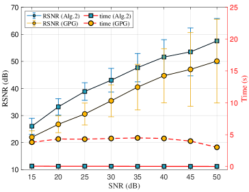
Figure 3.1: Comparison of Algorithm 2 and GPG in accuracy (RSNR) and time for different SNRs (averaged over 100 runs).

Experiment 2.

(support accuracy) We choose a similar setup as in Experiment 1. We test on different sizes for the matrix $\mathbf{A}$ under a fixed SNR = $50$. The original vector $\boldsymbol{x}^{*}$ is generated with approximately 4% nonzero entries.

To quantitatively assess the performance of the algorithms in recovering the support of $\boldsymbol{x}^{*}$, we employ a confusion matrix with a detailed definition in Table 3.1 and compute various metrics, including accuracy, precision, recall, and the F1 score shown below.

		Actual
		Nonzero	Zero
Predicted	Nonzero	True positive (TP)	False positive (FP)	Precision $\frac{\text{TP}}{\text{TP}+\text{FP}}$
	Zero	False negative (FN)	True negative (TN)
	Recall $\frac{\text{TP}}{\text{TP}+\text{FN}}$		Accuracy $\frac{\text{TP}+\text{TN}}{\text{TP}+\text{FN}+\text{FP}+\text{TN}}$
$\textbf{F1}=\displaystyle{2\times\textbf{Precision}\times\textbf{Recall}\over\textbf{Precision}+\textbf{Recall}}$

Table 3.1: Confusion matrix metrics

In our numerical experiment, we set $\varepsilon_{1}=\varepsilon_{2}=10^{-7}$ in Algorithm 2. For the parameters in GPG, we choose a similar setup as in Experiment 1 except for $\texttt{ITmax}=2000$. For the regularization parameters $\lambda$ in Algorithm 2 and $\lambda_{0}$ in GPG [30], we choose the values such that the predicted number of the nonzero elements in the estimated $\hat{\boldsymbol{x}}$ is approximately equal to the actual number of the nonzero elements in $\boldsymbol{x}^{*}$.

The comparative evaluation of the two algorithms is presented in Table 3.2. The results indicate that both algorithms exhibit a high accuracy, signifying their ability to find sparse solutions, given that most elements in $\boldsymbol{x}^{*}$ are zero. Nevertheless, Algorithm 2 demonstrates significantly enhanced precision, recall, and F1 scores compared to GPG. Specifically, for the nonzero elements within $\boldsymbol{x}^{*}$, GPG recovers only half of them, while our algorithm achieves nearly perfect recovery according to their recall and precision. In addition, Algorithm 2 attains substantially lower objective function values within a shorter time.

		accuracy	precision	recall	F1	time (s)	$\frac{1}{2}\|\mathbf{A}\hat{\boldsymbol{x}}-\boldsymbol{b}\|^{2}$
I	Alg. 2	0.994	0.969	0.939	0.949	0.017	$\mathbf{6.50\times 10^{-4}}$
	GPG [30]	0.962	0.556	0.504	0.520	0.088	$2.578\times 10^{-1}$
II	Alg. 2	0.999	0.990	0.988	0.989	0.241	$\mathbf{2.188\times 10^{-5}}$
	GPG [30]	0.961	0.511	0.496	0.501	1.778	$3.656\times 10^{-1}$

Table 3.2: Performance based on different metrics under case I ($\mathbf{A}_{50\times 300}$) and case II ($\mathbf{A}_{170\times 900}$) (average over 100 runs).

The efficacy of Algorithm 2 is vividly depicted in Figure 3.2, which presents a comprehensive overview of the metric performances across various dimensions of the matrix $\mathbf{A}$. Irrespective of the matrix size, Algorithm 2 consistently exhibits high accuracy, suggesting its robust ability to identify TP and TN with remarkable accuracy. In addition, a noteworthy observation is the upward trend in all metrics as the row dimension of the matrix $\mathbf{A}$ expands, especially for the precision, recall, and F1. Finally, as the ratio of the number of rows to the number of columns approaches approximately $0.18$, Algorithm 2 demonstrates a remarkable capability to recover the ground truth vector $\boldsymbol{x}^{*}$.

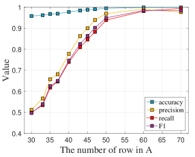
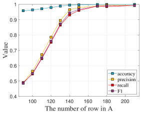
Figure 3.2: (Left) Metrics performance under fixed 300 columns in $\mathbf{A}$ (average over 100 runs). (Right) Metrics performance under fixed 900 columns in $\mathbf{A}$ (average over 100 runs)

Experiment 3.

(efficacy of the L0BPG step in Algorithm 2) We validate the efficacy of Algorithm 2 in picking an element that was not ranked high during the initialization phase. We choose a similar setup as in Experiment 1 with $\mathbf{A}\in\mathbb{R}^{60\times 300}$ without noise. The original vector $\boldsymbol{x}^{*}$ has $15$ nonzero entries, and we will get a vector with $N(<15)$ nonzero elements with the sparsity penalty.

We set $\lambda=1.5$, $N=12$ and $\varepsilon_{1}=\varepsilon_{2}=10^{-8}$. We plot the numerical changes of four elements (12th to 15th largest components in $\boldsymbol{x}^{*}$) in Figure 3.3. Note that we rank the four elements based on the original vector $\boldsymbol{x}^{*}$, and the figure shows that Algorithm 2 picks the original 14th largest element instead of the 12th one.

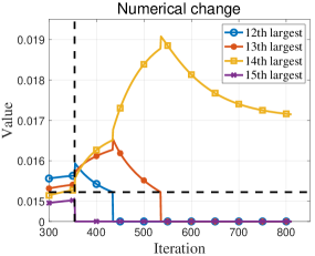
	Alg. 2 keep 14th	keep 12th
$\frac{1}{2}\|\mathbf{A}\hat{\boldsymbol{x}}-\boldsymbol{b}\|^{2}$	0.0176	0.0191

Figure 3.3: (Left) The numerical changes of the four elements ranked from the 12th to the 15th largest of the original $\boldsymbol{x}^{*}$ in Algorithm 2. The dashed vertical and horizon lines indicate the completion of the initialization phase and the minimal value controlled, i.e., $1-e^{-\alpha\lambda}$, respectively. (Right) The error comparison for including the 14th and the 12th elements of $\boldsymbol{x}^{*}$, where $\hat{\boldsymbol{x}}$ is the output vector. Both vectors contain the first 11 largest elements in $\boldsymbol{x}^{*}$.

Given that Algorithm 2 outputs a vector with 12 nonzero elements, we further substantiate that the 14th largest element in $\boldsymbol{x}^{*}$ outperforms the 12th by solving the problem without the sparsity penalty, yet preserving only the top 12 largest elements in $\boldsymbol{x}^{*}$. Both vectors contain the first 11 largest elements in $\boldsymbol{x}^{*}$, and Figure 3.3 shows that including the 14th one has a smaller error than that including the 12th one, which validates the efficacy of Algorithm 2.

3.2 Sparse portfolio optimization

We consider the following portfolio optimization problem:

$$\min_{\boldsymbol{x}\in\mathbb{R}^{n}} \frac{1}{2}\eta\left(\boldsymbol{x}^{\top}\mathbf{\Sigma}\boldsymbol{x}\right)-(1-\eta)\left(\boldsymbol{\mu}^{\top}\boldsymbol{x}\right)$$ (3.1)

subject to $$\mathbf{1}^{\top}\boldsymbol{x}=1,\boldsymbol{x}\geq 0,$$

where $\boldsymbol{\mu}$ and $\mathbf{\Sigma}$ are the expected return and the covariance matrix of the $n$ assets, respectively. Portfolio optimization aims to maximize the expected return ($\boldsymbol{\mu}^{\top}\boldsymbol{x}$) while minimizing the risk ($\boldsymbol{x}^{\top}\mathbf{\Sigma}\boldsymbol{x}$), and the risk aversion parameter $\eta$ balances both objectives. By varying $\eta\in[0,1]$, the optimization problem returns different portfolios that form the efficient frontier in the context of Markowitz’s theory [23]. There are mainly two types of efficient frontiers [16]: the standard efficient frontier, which solves the problem (3.1), and the general efficient frontier, which solves the same problem with an additional sparsity constraint $\|\boldsymbol{x}\|_{0}\leq K$ for a given $K$.

We use the benchmark datasets for portfolio optimization from the OR-Library. The datasets have weekly prices of some assets from five financial markets (Hang Seng in Hong Kong, DAX 100 in Germany, FTSE 100 in the UK, S&P 100 in the USA, and Nikkei 225 in Japan) between March 1992 and September 1997. The numbers of assets in the five markets were 31, 85, 89, 98, and 225, respectively. We choose 2000 and 50 evenly spaced $\eta$ values for the standard efficient frontiers (SEF) and the general efficient frontiers (GEF), respectively. We also set $K=10$ in the general efficient frontier. To compare these two frontiers, we employ three criteria: mean Euclidean distance, variance of return (risk) error, and mean return error [32, 13]. These three metrics describe the overall distance between these two frontiers, the risk’s relative error, and the mean return’s relative error. They are referred to as distance, variance, and mean, respectively, in Table 3.3.

Table 3.3 demonstrates that the general efficient frontier closely approximates the standard efficient frontier, as indicated by the low values of mean Euclidean distance, variance of return error, and mean return error. We also plot the general and standard efficient frontier in Figure 3.4, which visualizes the distance between these two frontiers. In these figures, the points with sparsity 10 are still very close to the curve without sparsity.

index	Hang Seng	DAX 100	FTSE 100	S&P 100	Nikkei
assets	31	85	89	98	225
distance ($\times 10^{-6}$)	$1.683$	$1.311$	$1.269$	$9.448$	$1.583$
variance (%)	0.058	0.251	0.248	0.637	0.043
mean (%)	0.0263	0.027	0.025	0.527	1.970
time (s)	0.397	0.549	0.509	0.720	13.761

Table 3.3: The numerical results for sparse portfolio optimization problem. The last row is the total time for calculating these two frontiers.

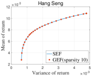
(a)

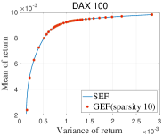
(b)

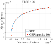
(c)

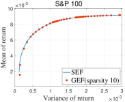
(d)

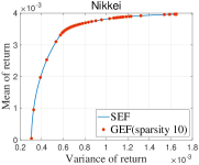
(e)

Figure 3.4: (a) Efficient frontier for Hang Seng. (b) Efficient frontier for DAX 100. (c) Efficient frontier for FTSE 100. (d) Efficient frontier for S&P 100. (e) Efficient frontier for Nikkei.

4 Conclusion

This paper addresses the $\ell_{0}$-sparse optimization problem subject to a probability simplex constraint. We introduce an innovative algorithm that leverages the Bregman proximal gradient method to progressively induce sparsity by explicitly solving the associated subproblems. Our work includes a rigorous convergence analysis of this proposed algorithm, demonstrating its capability to reach a local minimum with a convergence rate of $O(1/k)$. Additionally, the empirical results illustrate the superior performance of the proposed algorithm. Finally, Future work will delve into strategies for reintroducing important elements that have been set to zero during the algorithmic process and the design of an adaptive regularized parameter.

Declarations

Acknowledgements This work was partially supported by the Guangdong Key Lab of Mathematical Foundations for Artificial Intelligence and Shenzhen Science and Technology Program ZDSYS20211021111415025.

Data availability The data generated in Subsection 3.1 are available at https://github.com/PanT12/Efficient-sparse-probability-measures-recovery-via-Bregman-gradient.
The data that support Subsection 3.2 are openly available in http://people.brunel.ac.uk/~mastjjb/jeb/orlib/portinfo.html.
Conflict of interest The authors declare that they have no conflict of interest.

References

- [1] Auslender, A., Teboulle, M.: Interior gradient and proximal methods for convex and conic optimization. SIAM Journal on Optimization 16(3), 697–725 (2006)
- [2] Bauschke, H.H., Bolte, J., Teboulle, M.: A descent lemma beyond Lipschitz gradient continuity: first-order methods revisited and applications. Mathematics of Operations Research 42(2), 330–348 (2017)
- [3] Beck, A., Teboulle, M.: Mirror descent and nonlinear projected subgradient methods for convex optimization. Operations Research Letters 31(3), 167–175 (2003)
- [4] Beck, A., Teboulle, M.: Gradient-based algorithms with applications to signal recovery. Convex optimization in signal processing and communications pp. 42–88 (2009)
- [5] Ben-Tal, A., Margalit, T., Nemirovski, A.: The ordered subsets mirror descent optimization method with applications to tomography. SIAM Journal on Optimization 12(1), 79–108 (2001)
- [6] Bertsimas, D., Cory-Wright, R.: A scalable algorithm for sparse portfolio selection. Informs journal on computing 34(3), 1489–1511 (2022)
- [7] Birnbaum, B., Devanur, N.R., Xiao, L.: Distributed algorithms via gradient descent for Fisher markets. In: Proceedings of the 12th ACM conference on Electronic commerce, pp. 127–136 (2011)
- [8] Blumensath, T., Davies, M.E.: Iterative thresholding for sparse approximations. Journal of Fourier analysis and Applications 14, 629–654 (2008)
- [9] Blumensath, T., Davies, M.E.: Iterative hard thresholding for compressed sensing. Applied and computational harmonic analysis 27(3), 265–274 (2009)
- [10] Blumensath, T., Davies, M.E.: Normalized iterative hard thresholding: Guaranteed stability and performance. IEEE Journal of selected topics in signal processing 4(2), 298–309 (2010)
- [11] Bolte, J., Sabach, S., Teboulle, M., Vaisbourd, Y.: First order methods beyond convexity and Lipschitz gradient continuity with applications to quadratic inverse problems. SIAM Journal on Optimization 28(3), 2131–2151 (2018)
- [12] Boyd, S.P., Vandenberghe, L.: Convex optimization. Cambridge university press (2004)
- [13] Cura, T.: Particle swarm optimization approach to portfolio optimization. Nonlinear analysis: Real world applications 10(4), 2396–2406 (2009)
- [14] Eckstein, J.: Nonlinear proximal point algorithms using Bregman functions, with applications to convex programming. Mathematics of Operations Research 18(1), 202–226 (1993)
- [15] Esmaeili Salehani, Y., Gazor, S., Kim, I.M., Yousefi, S.: -norm sparse hyperspectral unmixing using arctan smoothing. Remote Sensing 8(3), 187 (2016)
- [16] Fernández, A., Gómez, S.: Portfolio selection using neural networks. Computers & operations research 34(4), 1177–1191 (2007)
- [17] Fornasier, M., Rauhut, H.: Compressive sensing. Handbook of mathematical methods in imaging 1, 187–229 (2015)
- [18] Hanzely, F., Richtarik, P., Xiao, L.: Accelerated Bregman proximal gradient methods for relatively smooth convex optimization. Computational Optimization and Applications 79, 405–440 (2021)
- [19] Jiang, X., Vandenberghe, L.: Bregman three-operator splitting methods. Journal of Optimization Theory and Applications 196(3), 936–972 (2023)
- [20] Krichene, W., Bayen, A., Bartlett, P.L.: Accelerated mirror descent in continuous and discrete time. Advances in neural information processing systems 28 (2015)
- [21] Lu, H., Freund, R.M., Nesterov, Y.: Relatively smooth convex optimization by first-order methods, and applications. SIAM Journal on Optimization 28(1), 333–354 (2018)
- [22] Ma, S., Goldfarb, D., Chen, L.: Fixed point and Bregman iterative methods for matrix rank minimization. Mathematical Programming 128(1-2), 321–353 (2011)
- [23] Markowits, H.M.: Portfolio selection. Journal of finance 7(1), 71–91 (1952)
- [24] Natarajan, B.K.: Sparse approximate solutions to linear systems. SIAM journal on computing 24(2), 227–234 (1995)
- [25] Nemirovskij, A.S., Yudin, D.B.: Problem complexity and method efficiency in optimization (1983)
- [26] Pan, L., Zhou, S., Xiu, N., Qi, H.D.: A convergent iterative hard thresholding for nonnegative sparsity optimization. Pacific Journal of Optimization 13(2), 325–353 (2017)
- [27] Salehani, Y.E., Gazor, S., Kim, I.M., Yousefi, S.: Sparse hyperspectral unmixing via arctan approximation of L0 norm. In: 2014 IEEE Geoscience and Remote Sensing Symposium, pp. 2930–2933. IEEE (2014)
- [28] Tang, W., Shi, Z., Duren, Z.: Sparse hyperspectral unmixing using an approximate L0 norm. Optik 125(1), 31–38 (2014)
- [29] Tibshirani, R.: Regression shrinkage and selection via the lasso. Journal of the Royal Statistical Society Series B: Statistical Methodology 58(1), 267–288 (1996)
- [30] Xiao, G., Bai, Z.J.: A geometric proximal gradient method for sparse least squares regression with probabilistic simplex constraint. Journal of Scientific Computing 92(1), 22 (2022)
- [31] Xu, L., Lu, C., Xu, Y., Jia, J.: Image smoothing via L0 gradient minimization. In: Proceedings of the 2011 SIGGRAPH Asia conference, pp. 1–12 (2011)
- [32] Yin, X., Ni, Q., Zhai, Y.: A novel PSO for portfolio optimization based on heterogeneous multiple population strategy. In: 2015 IEEE Congress on Evolutionary Computation (CEC), pp. 1196–1203. IEEE (2015)
- [33] Zhang, J.Y., Khanna, R., Kyrillidis, A., Koyejo, O.O.: Learning sparse distributions using iterative hard thresholding. Advances in Neural Information Processing Systems 32 (2019)
- [34] Zhang, P., Xiu, N., Qi, H.D.: Sparse SVM with hard-margin loss: a Newton-augmented lagrangian method in reduced dimensions. arXiv preprint arXiv:2307.16281 (2023)
- [35] Zhao, C., Xiu, N., Qi, H., Luo, Z.: A Lagrange–Newton algorithm for sparse nonlinear programming. Mathematical Programming 195(1-2), 903–928 (2022)
- [36] Zhou, S., Xiu, N., Qi, H.D.: Global and quadratic convergence of Newton hard-thresholding pursuit. The Journal of Machine Learning Research 22(1), 599–643 (2021)