Simulations of galaxies in an expanding Universe with modified Newtonian dynamics (MOND) and with modified gravitational attractions (MOGA)

Abstract

The stability of galaxies is either explained by the existence of dark matter or caused by a modification of Newtonian acceleration (MOND). Here we show that the modification of the Newtonian dynamics can equally well be obtained by a modification of Newton’s law of universal gravitational attraction (MOGA), by which an inverse square attraction from a distant object is replaced with an inverse attraction. This modification is often proposed in the standard model, and with the modification of the attraction caused by dark matter. The recently derived algorithm, Eur. Phys. J. Plus 137 99 (2022); Class. Quantum Grav. 39 225006 (2022), for classical celestial dynamics is used to simulate models of the Milky Way in an expanding universe and with either MOND or MOGA. The simulations show that the galaxies with MOND dynamics are unstable whereas MOGA stabilizes the galaxies. The rotation velocities for objects in galaxies with classical Newtonian dynamics decline inversely proportional to the square root of the distance $r$ to the center of the galaxy. But the rotation velocities is relatively independent of $r$ for MOGA and qualitatively in agreement with experimentally determined rotation curves for galaxies in the Universe. The modification of the attractions may be caused by the masses of the objects in the central part of the galaxy by the lensing of gravitational waves from far-away objects in the galaxy.

I Introduction.

The evolution of the Universe, the kinematics, and the stability of galaxies is usually explained by the presence of Dark Matter (DM) Swart2017 . The standard model used is the $\Lambda$ Cold Dark Matter ($\Lambda$CDM) model, in which the galaxies’ rotation velocities as well as their stability is ensured by DM Bullock2017 ; Perivolaropoulos2022 . The Newtonian inverse square gravitational attraction from baryonic matter is, however, not included in the standard model, and this has given rise to a series of proposed modifications of Newton’s inverse square law (ISL) for gravitational attraction with the intention of unifying gravity with particle physics Fischbach2001 ; Adelberger2003 ; Lee2020 ; Henrichs2021 .

The rotation velocities of galaxies deviate from the Classical Mechanics rotation velocities Rubin1980 ; Rubin1985 ; Gentile2011 ; Corbelli2000 which decline inversely proportional to the square root of the distance $r$ to the center of the galaxy. This behavior is taken into account in the theories that have led to the assumption of the existence of DM in the Universe Bertone2018 . Another attempt to explain the stability and the dynamics of galaxies is the MOND theory, where the stability of the galaxies and their rotation velocities is caused by modified Newtonian dynamics at small accelerations Milgrom1983 . The Newtonian dynamics can either be changed by modifying the accelerations of baryonic objects at small accelerations (MOND) or by modifying the gravitational attractions (MOGA) from objects located far away Bekenstein1984 . The MOND theory is reviewed in Famaey2012 .

Modifications of the gravitational attraction (MOGA) have been proposed for a long time, and modified gravity are reviewed in Clifton2012 ; Mendoza2015 . The modification could be caused by the general relativistic gravitational lensing (GL) which deals with the effect of wave deflection caused by baryonic objects. GL is reviewed in Bartelmann2010 ; Mukherjee2021 . Gravitational waves were first detected in 2016 Abbott2016 . Simultaneously detection of gravitational and electromagnetic waves from the coalescence of binary neutron stars rules, however, out a class of MOND theories Boran2018 .

The kinematics of the galaxies is determined by radiation from the galaxies or by simulations. Simulations of galaxies have been performed for many decades. The dynamics of baryonic objects can be solved by the Particle-Particle/Particle-Mess (PPPM) method Hockney1974 ; Klypin1983 ; Centrella1983 , which is a mean-field approximation where each mass unit is moving in the collective field of all the others, and the Poison equation for the PPPM grid is solved numerically. The dynamics are determined for Zeldovich’s adiabatic expansion of the Einstein-de Sitter universe Zeldovich1970 . Later, simulations with large scaled computer packages with PPPM (GADGET, PHANTOM, RAMSES, AREPO) Springel2005 ; Price2018 ; Weinberger2020 are with many billions of mass units. The evolution of galaxies has been obtained from hydrodynamical large-scaled cosmological simulations Schaye2010 ; Dubois2014 ; Vogelsberger2014 , and with co-evolving dark matter gas and stellar objects Dubois2016 ; Ludlow2021 . Simulations of galaxies with MOND dynamics have also been performed by (approximated) Poisson solvers and Angus2014 ; Angus2014a ; Lughausen2014 . Cosmological simulations of galaxy formation are reviewed in Vogelsberger2020 .

Here we simulate models of galaxies with the modified Newtonian dynamics, MOND, and with modified gravitational attraction, MOGA. The MOND acceleration is obtained from the interpolation function(s) Milgrom1983 ; Gentile2011 , and the modified gravitational attraction, MOGA, is obtained by replacing Newton’s gravitational inverse square attraction (ISL) with an inverse attraction (IA) for large distances. The simulations of galaxies in an expanding Universe are performed by use of a recent extension of Newton’s discrete algorithm Newton1687 ; Toxvaerd2020 ; Toxvaerd2022 ; Toxvaerd2022a . The algorithm is absolutely stable and without any approximations, and the dynamics with the discrete algorithm have the same invariances as Newton’s analytic dynamics, and thus the discrete dynamics is exact in the same sense as the exact solution of Newton’s analytic second-order differential equations for classical celestial mechanics. The dynamics with Newton’s discrete algorithm is reviewed in Toxvaerd2023 , and the algorithm and the proof that Newton’s discrete dynamics has the same invariances as his analytic dynamics is given in the Appendix. The advantage of using Newton’s discrete algorithm is that the classical dynamics are without any approximations, and the disadvantage is that it is only possible to perform the exact long-time simulations for small ensembles of objects in bound rotations around their common mass center.

The Newtonian dynamics with MOND and with MOGA are formulated in the next section. The acceleration in MOND is modified when the acceleration of an object is below a certain threshold, $a_{0}$, and $independent$ of the individual attractions from the objects which together cause the small acceleration. Unlike MOGA, MOND no longer conserves the momentum and angular momentum for a conservative system(see the Appendix, Eq. (A.7), Figure A.1, and Felten1984 ), and the present simulations reveal that MOND is unstable. Section 3 presents the results of the MOND and MOGA simulations of galaxies for times corresponding to the age of the Universe. The simulations show that the MOND dynamics is unstable and releases the bound objects in the galaxies with time, whereas MOGA not only stabilizes the bound rotations of the objects in the galaxies but also changes the rotation velocities in the way proposed by Milgrom Milgrom1983 ; Bekenstein1984 .

II Modified acceleration, MOND, and modified gravitational attraction, MOGA.

Newtonian dynamics for celestial objects is given by Newton’s classical dynamics and his ISL law of gravitation

$$\textbf{F}_{i}(t)=m_{i}\textrm{a}_{i}\hat{\textbf{a}}_{i}(t)=\textrm{F}_{i}\hat{\textbf{a}}_{i}=-\sum_{j\neq i}^{N}{\frac{m_{i}m_{j}G}{r_{ij}^{2}(t)}\hat{\textbf{r}}_{ij}(t)}$$ (1)

for the force $\textbf{F}_{i}(t)$ and the acceleration $\textbf{a}_{i}(t)=\textrm{a}_{i}\hat{\textbf{a}}_{i}(t)$ for the object $i$ in the ensemble of $N$ objects, caused by baryonic objects $j$ with mass $m_{j}$ at distances $r_{ij}(t)$ and at time $t$.

The MOND theory was published in 1983 by M. Milgrom Milgrom1983 . The acceleration $\textbf{a}_{i}(t)$ in classical Newtonian dynamics is modified for a small acceleration caused by the sum of interactions with the $N-1$ baryonic objects located at large distances $r_{ij}$ from $i$. The transition from the Newtonian acceleration to MOND occurs for a small acceleration $a_{i}\approx a_{0}=\mid\textbf{a}_{0}\mid$. This can only happen if $all$ the attractions with object $i$ from the other $N-1$ baryonic objects are for large distances so that the sum of attractions results in a small acceleration $a_{i}<a_{0}$

$$a_{i}\rightarrow\mu(a_{i}/a_{0})a_{i}.$$ (2)

According to Bekenstein and Milgrom Bekenstein1984 the modification can either be performed by modifying the law of inertia (MOGA) or by modifying the acceleration (MOND). The modification, $\mu$, of the acceleration $\mid\textbf{a}_{i}\mid$ is obtained with the ”standard interpolation function”

$$\mu(\textrm{a}/a_{0})=\sqrt{\frac{1}{1+(\frac{a_{0}}{\textrm{a}})^{2}}},$$ (3)

The MOND acceleration is given by

$$\textrm{F}_{i}/m_{i}=\textrm{a}_{i}\sqrt{\frac{\textrm{a}_{i}^{2}}{\textrm{a}_{i}^{2}+a_{0}^{2}}},$$ (4)

or the interpolation function proposed by Gentile2011

$$\mu(\textrm{a}/a_{0})=\frac{\mid\textrm{a}\mid}{\mid\textrm{a}\mid+a_{0}},$$ (5)

with the modification given by

$$\textrm{F}_{i}/m_{i}=\textrm{a}_{i}\frac{\mid\textrm{a}_{i}\mid}{\mid\textrm{a}_{i}\mid+a_{0}},$$ (6)

and acceleration

$$\textrm{a}_{i}(\textrm{MOND})=\frac{\textrm{F}_{i}}{2m_{i}}(1+\sqrt{1+4m_{i}a_{0}/\mid\textrm{F}_{i}\mid}).$$ (7)

The MOND modifications, Eq. (4) or Eq. (6), change the acceleration from the classical Newtonian acceleration $\mid\textbf{a}\mid>>a_{0}$ at short distances to a modified acceleration

$$\mid\textbf{a}_{i}(\textrm{MOND})\mid=\sqrt{\mid\textrm{F}_{i}\mid a_{0}/m_{i}}$$ (8)

for $\mid\textbf{a}\mid<<a_{0}$.

The asymptotic modified acceleration for an isolated object $i$ with only one gravitational interaction, $\textrm{F}_{i}(r_{ij})=-m_{i}m_{j}G/r_{ij}^{2}$, with another object, No. $j$, is obtained from F${}_{i}(r_{ij})$ and Eq.(8) as

$$\textrm{a}_{i}(\textrm{MOND})=-\frac{\sqrt{m_{j}Ga_{0}}}{r_{ij}}.$$ (9)

MOND is a modification of Newtonian acceleration. But in this case, the modification might as well be formulated as a modification of Newton’s ISL law of universal gravitational attraction, where the inverse square attraction asymptotically is replaced with an inverse attraction (IA). If this modified gravitational attraction is a universal law, MOGA, the gravitational force is modified to

$$\textbf{F}_{i}(\textrm{MOGA})=-\sum^{N}_{j\neq i}\frac{m_{i}m_{j}G}{r_{ij}^{2}}(1+\frac{r_{ij}}{r_{0}})\hat{\textbf{r}}_{ij}(t)$$ (10)

with $r_{0}=\sqrt{m_{j}G/a_{0}}$.

The modified gravitational attraction, Eq. (10), is a specific example of a general modification of the force field Bekenstein1984 . Newtonian dynamics and Newton’s discrete algorithm used in the next section are time reversible, symplectic and with the dynamical invariances: momentum, angular momentum, and energy for a conservative system Toxvaerd2023 . MOGA with Newton’s discrete algorithm, maintains these qualities, whereas MOND does not conserve momentum and angular momentum (see Appendix A.2 and Figure A1) Felten1984 . The Hubble expansion of the space destroys the invariances Toxvaerd2022a , but MOND and MOGA dynamics are, however, still time reversible.

Modifications of the Newtonian ISL attraction have been proposed for a long time in an attempt to obtain the stability of galaxies by the standard model Fischbach2001 ; Adelberger2003 ; Henrichs2021 . The Newtonian gravitational potential $u(r)$ is modified by a Yukawa potential

$$v_{ij}(r)=u(r_{ij})[1+\alpha exp(-r_{ij}/\lambda)],$$ (11)

and the corresponding modified gravitational forces are

$$\textrm{F}_{i}=-\sum^{N}_{j\neq i}\frac{m_{i}m_{j}G}{r_{ij}^{2}}[1+\alpha exp(-r_{ij}/\lambda)(1+r_{ij}/\lambda)].$$ (12)

The parameter $\lambda$ corresponds to the parameter $r_{0}$ in MOGA, and a possible deviation from the ISL gravity was investigated for $\lambda$ in the range $\lambda\in[30,8000]$ nm Chen2016 ; Bimonte2021 ; Baeza-Ballesteros2022 , and the rotation velocities of stars in the Milky Way were used to determine a possible Yukawa correction, Eq. (11) to the gravitational attraction Henrichs2021 . So far, however, there is no direct experimental evidence for deviation from the ISL gravitational attraction.

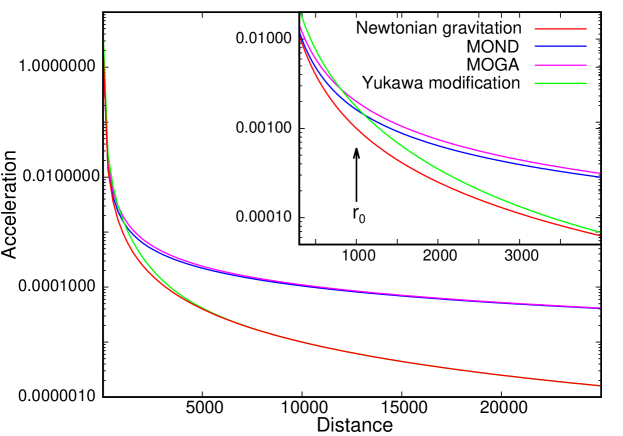
Figure 1: An illustrative figure of the modified accelerations a=F/$m$ of an object as a function of the distance $r$ to a heavy object with a mass $M=1000m$. Length unit is in parsec and force (F=$mMG/r^{2})$ is in units of $m$ and $G$. The MOND acceleration (Eq. 7) is in blue, the MOGA acceleration (Eq. 10) is in magenta, and the acceleration with the modified Yukawa attraction (Eq. 12) is in green. The accelerations are for $r_{0}=\lambda$=1000 parsec. The Newtonian acceleration with the ISL (Eq. 1) is shown in red. The inset enlarges the differences at $r\approx r_{0}$.

An illustrative example of the different accelerations are shown in Figure 1. (Units are with $m_{i}=G=1$ and length unit $1$ corresponds to 1 pc for a galaxy. For units see Toxvaerd2022a ). The accelerations are for $one$ object attracted by a heavy mass center with a mass that is a thousand times heavier than the object and for a modification distance $r_{0}=\lambda=1000$, which corresponds to 1 kpc for the model for the Milky Way in the next section. The Yukawa modification is shown in green, the MOND acceleration is in blue, and the MOGA acceleration in magenta. The MOND and MOGA modifications are rather similar in this case, but MOGA and MOND for galaxies with many gravitational objects are, however, very different. The difference between MOGA and MOND for the dynamics of a galaxy originates from the summation of interactions between the objects. The acceleration in MOND is modified if the interactions of an object with $all$ the other baryonic objects result in an acceleration below a certain threshold, whereas the contribution to the acceleration from the attractions of all faraway objects is modified in MOGA. The green curve is the force from the modification with the Yukawa potential, Eq. (12), and with $\alpha=1$ and $\lambda=$1000. If there exist dark matter this modified force will be effective on a much shorter length scale with baryonic attractions from dark matter in the galaxies and their halos.

The mean rotation velocities of stars in galaxies are rather constant and independent of the distance to the centers of rotation as opposed to a system of rotating baryonic objects with classical Newtonian dynamics Milgrom1983 ; Gentile2011 . This led Milgrom to propose the modification, Eq. (3) (or Eq. (5)) of the Newtonian classical acceleration, and with the asymptotic modification Eq. (8). By adjusting the modified acceleration to one (isolated) baryonic object in rotation at a gravitational center he determined a value for the constant $a_{0}$. Milgrom found $a_{0}\approx 1.2\times 10^{-10}$ ms^-2 to be optimal, and later investigation of the rotation curves for stars in 12 galaxies confirmed this value Gentile2011 . For a MOND modification caused by only one baryonic object with mass $m_{j}$ equal to the mass of our Sun: $m_{j}=m_{\textrm{Sun}}$=1.989$\times 10^{30}$ kg and with the gravitational constant $G=6.647\times 10^{-11}$ N m² kg^-2 the constant $a_{0}$ corresponds to a distance

$$r_{0}=\sqrt{\frac{m_{j}G}{a_{0}}}=\sqrt{\frac{1.99\times 10^{30}\times 6.65\times 10^{-11}}{1.2\texttimes 10^{-10}}}$$

$$=1.05\times 10^{15}\textrm{m}=\frac{1.05\times 10^{15}\textrm{m}}{3.09\times 10^{16}\textrm{m}\textrm{parsec}^{-1}}$$

$$=0.033\textrm{parsec},$$ (13)

The example is for one interaction from an object with mass equal to our Sun. The modification distance is proportional with the square root of the masses, $m_{j}$, and the distance is much larger for a modification caused by many heavy objects far away. The Milky Way is a barred spiral galaxy. The extension of the barred disk is 2.5-3 kpc Rix2013 and the extension of the halos is $\approx$ 100-300 kpc Deason2020 ; Li2021 , so the galaxy will be affected by a modification of the gravitational attractions or the accelerations.

III Simulations of galaxies with MOGA and with MOND.

Simulations of galaxies have been performed for many decades Aerseth1963 , but the simulations here of models of galaxies deviate from the main part of the simulations in that they are pure Newtonian N-body simulations. Such simulations have, however, also been simulated for a long time. But one has performed a series of approximations, such as variable time steps and mean field approximations, because these simulations are very time-consuming. But the approximations ruin the exactness of the simulations. The simulations below are exact N-body Newtonian simulations without any approximations. The algorithm with the conserved dynamic invariances is given in the Appendix and in a recent review article about Newton’s exact discrete dynamics Toxvaerd2023 .

A galaxy and the Milky Way contain hundreds of billions of stars, and a substantial amount of baryonic gas Gupta2012 ; Bergma2018 , and it is not possible to obtain the exact dynamics with MOGA or with MOND of a galaxy with this number of objects. We have instead of simulated models of small ”galaxies” of hundred of objects in orbits around their center of gravity, and in an expanding space with various values of $r_{0}$ or $a_{0}$. A recent article describes how a system of baryonic objects with Newtonian discrete dynamics spontaneously creates a system with the objects in rotation about their center of gravity Toxvaerd2022 . The algorithm is extended to also include the dynamics with the Hubble expansion of the space Toxvaerd2022a . (The relations between the units for length $l$: 1 pc, time $t$: 1 Gyr and Hubble expansion coefficient $H=72.1\pm 2.0\ \textrm{km}\textrm{s}^{-1}\textrm{Mpc}^{-1}$ Soltis2021 in the Universe and the corresponding units for the MD models of galaxies are: 1 pc $\hat{=}$ 1 MD length unit, 1 Gyr $\hat{=}6\times 10^{5}$ MD time units and $72.1\textrm{km}\textrm{s}^{-1}\textrm{Mpc}^{-1}\hat{=}5.\times 10^{-8}$ in MD units Toxvaerd2022a .)

The algorithm is used to simulate models of a galaxy with the Hubble expansion and with MOGA and MOND, respectively. An ensemble of gravitational objects with Newtonian dynamics at time $t$=0 might spontaneously create a ”galaxy” system with many of the objects in a bound rotation around the center of gravity, and one can either start the simulations with MOGA or MOND at $t=0$, or alternatively at a later time $t$ where a Newtonian galaxy is created and it is in a rather stable state. The data reported below for twelve galaxies are started from a stable Newtonian galaxy. The twelve galaxies with the data reported below are for $r_{0}=1,10,100,1000,10000,100000$ and $a_{0}=1,10^{-2},10^{-4},10^{-6},10^{-8},10^{-10},$ respectively, and each (stable) galaxy are simulated $3.2\times 10^{9}$ time steps corresponding to $t=8\times 10^{6}\approx$ 13.4 Gyr or the age of the Universe. Each simulation with the $3.2\times 10^{9}$ time steps took $\approx$ 1000 hours on a fast CPU in the CPU-cluster, and the total amount of simulations for different values of $r_{0},a_{0},H$, and start configurations is fifty-three.

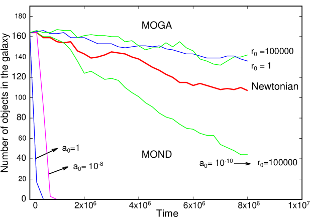
Figure 2: The number of objects with mean distances $r(\textrm{mean})<100000$ parsec to the center of mass as a function of time $t\in[0,8\times 10^{6}]\approx$ 13.4 Gyr where the galaxies are exposed to either MOND or MOGA. The red curve is for Newtonian dynamics without any modification of accelerations or attractions. The green curves are for a very weak/long range modification $a_{0}=10^{-10}$ (MOND) corresponding to $r_{0}=100000$ (MOGA), and the blue curves are for a strong/short range modification $a_{0}=r_{0}=1$. The magenta curve is MOND dynamics with $a_{0}=10^{-8}$.

III.1 Stability of galaxies with MOGA or with MOND.

The dynamical effect of the modifications of the accelerations or gravitational forces is obtained by exposing the objects in a galaxy to MOGA or to MOND. The results reported below are obtained by exposing the objects in a Newtonian galaxy which is in a rather stable state and with an occasional release of an object before the modifications (Curve in red in Figure 2). At the start of the modifications the system contains 460 objects with 165 with a mean distances $r(\textrm{mean})<100000)$ parsec to the center of mass, and 295 objects with mean distances $r\textrm{(mean})>100000\approx 100$ kpc. The number of objects with mean distances $r(\textrm{mean})<100000)$ in the galaxy after the change of dynamics is shown in Figure 2.

The stars in the halos of a galaxy are not in a stable and bound rotation, and this fact has led to the hypothesis about the existence of dark matter in the Universe. The simulations of Newtonian galaxies show, however, that the release of stars in the outer edge of a Newtonian galaxy is rare, and that the Newtonian galaxies are rather stable over time periods of many Gyr (red curve in Figure 2) Toxvaerd2022a . By changing the Newtonian dynamics to MOND the enhanced MOND acceleration destabilizes the galaxy and results in a release of the bound objects, whereas the MOGA dynamics has the opposite effect. The number of bound objects with $r_{0}=a_{0}$=1 is shown in blue, and the number with $a_{0}=10^{-10}$ (MOND) and correspondingly $r_{0}$=100000 (MOGA) is shown in green in Figure 2. MOGA stabilizes the galaxy even for a very weak modification with $r_{0}\approx 10000-100000$ corresponding to a modification of the attractions at distances $\approx$ 10-100 kpc for the Milky Way. The galaxies with MOGA still release objects, but this is very rare and the galaxies contain still more than 135 bound objects after a time $\Delta t=8\times 10^{6}$ corresponding to 13.4 Gyr, or the age of the Universe. The simulations are performed for $r_{0}=1(136),10(143),100(142),1000(156),10000(156)$ and $100000(142)$, respectively, and with the number of objects with mean distances $r(\textrm{mean})<100000$ at the end of the simulations indicated in the parentheses. The number of objects in the Newtonian galaxy with $r_{0}=\infty$ at the end of the simulation (red curve in Figure 2) is $N=$107, so the MOGA galaxies contain significantly more bound objects than the Newtonian galaxy. The stability of the galaxy given by the number of bound objects with MOGA is not sensitive to the range $r_{0}$ of the modification of the gravitational attraction.

The number of bound objects ($r(\textrm{mean})<100000$) with MOND dynamics is also shown in Figure 2. The MOND dynamics releases the objects even for a very low threshold for the modified acceleration, given by $a_{0}=1/r_{0}^{2}$. It was only possible to maintain some bound objects for a very weak modification of the Newtonian accelerations with $a_{0}=10^{-10}\rightarrow r_{0}=100000$ (green MOND curve in Figure 2). All the bound objects were released for a stronger MOND modification of the acceleration.

Galaxies with MOGA or with MOND dynamics were simulated with other start distributions of the baryonic objects and for $H=0$ (i.e. without a Hubble expansion of the space). The simulations showed unanimously, that MOGA dynamics has a stabilizing effect on the objects in the galaxies even for a big value of $r_{0}$ corresponding to that only the stars in the halos of a galaxy are affected by the modified gravitational attraction. All the MOND simulations were unstable and released the bound objects sooner or later. MOND does not conserve the angular momentum of the ensemble (see Appendix A.2., Eqn. (A.7) and (A.9) and Figure A1), and the increased MOND acceleration has the opposite effect, it destabilizes the bound objects in the galaxies even for the very small value of $a_{0}=10^{-10}$ and the MOND galaxies release the objects from their regular orbits in the galaxies. The same was thru for dynamics without a Hubble expansion ($H=0$), where the galaxies were stable for MOGA, but unstable for MOND.

III.2 Rotation velocity of the stars in a galaxy.

There is a discrepancy between the mean rotation velocities of the stars in the galaxies and the corresponding mean velocities of the objects in the simulated galaxies with pure Newtonian dynamics. The mean rotation velocities of the stars in a galaxy as a function of the distance to the center of rotation increase for short distances, but are rather constant at larger distances to the center of the galaxies. Corbelli2000 ; Gentile2011 ; Famaey2005 . But the velocity $v(r)$ of objects with pure Newtonian dynamics in mean declines as $v(r)\approx(M/r)^{0.5}$ with the distance $r$ to the mass center of the galaxy with mass $M$. The rotation velocity of stars in the Milky Way at the distances $r\in[6.72,8.40]$ kpc is $v(r)\in[203,240]$ km s^-1 Camarillo2018 . One of the results in Toxvaerd2022a from the simulation of galaxies with pure Newtonian dynamics was, that the velocities of objects for distances $r\in[15000,100000]$ to the center were not located near a line with $v(r)=(M/r)^{0.5}$, but were diffusely distributed. But a determination of the rotation velocities over a longer time interval with the root mean square (rms), obtained from 22 consecutive time intervals of the mean velocities, reveals that the distribution of the mean rotation velocities is rather Newtonian, and disagrees with the $\approx$ constant rotation velocity in galaxies (Figure 3).

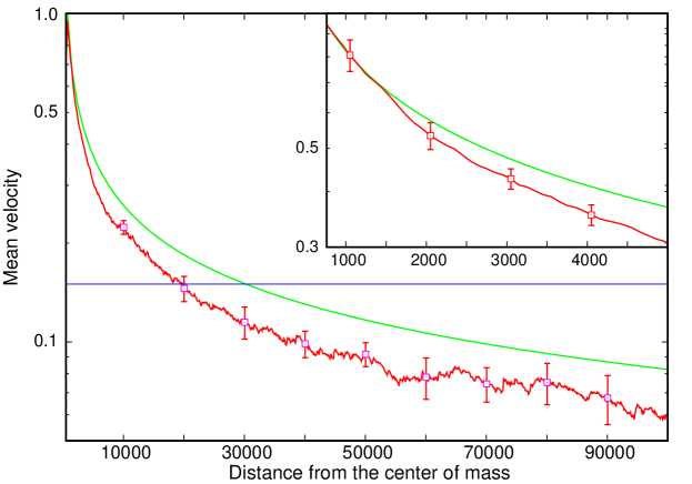
Figure 3: Mean rotation velocities of the objects in the galaxy with Newtonian dynamics in red (i.e. without a modification of accelerations or attractions). Distances are in parsec and velocities are in MD units where $v(r)=0.15$ corresponds to $v=220$ km/s in the Milky Way. In green is the Newtonian rotation velocity $v(r)=(M/r)^{0.5}$ for one bound object attracted by a heavy mass center. The blue line is $v(r)=0.15$. The standard deviations for (representative) selected distances are obtained from 22 consecutive time subsets of the mean rotation velocities in the subsets. The inset shows the mean velocities at short mean distances.

The rotation velocities of the objects in a galaxy with pure Newtonian dynamics is shown in Figure 3. The rotation velocities in red and standard deviation with magenta are obtained in the time interval $t\in[0,8\times 10^{6}]$. The green curve is the function $v(r)=(680/r)^{0.5}$ for one object in circulation around a mass center with a mass M=680 times the mass of the object. The blue straight line is $v=0.15$ and it corresponds to $v=220$ km/s for stars in the Milky Way Camarillo2018 . The rotation velocities decline even more rapidly with the distance to the center of rotation than given by $v(r)=(680/r)^{0.5}$, and in disagreement with the observed mean rotation velocities of the stars in galaxies.

The dynamics with MOGA increase the rotation velocities at distances $r>r_{0}$ to the center of the galaxy. The rotation velocities for MOGA dynamics and for different values of $r_{0}$ are shown in the next figure. The rotation velocities are for the bound objects with the distances $r<100000$. The mean velocities of the objects in Figure 4 are determined in the time interval $t\in[0,8\times 10^{6}]$. They are constant within the accuracy of the simulations already for a modified attraction with $r_{0}=10000$ corresponding to 10 kpc for the Milky Way and a smaller value of the distance $r_{0}$ for the onset of the modification only increases the constant mean velocity. So a modification of the ISL attraction to an inverse attraction not only stabilizes the galaxy, (Figure 2) but also increases the rotation velocities at large distances and make them rather constant with respect to the distance to the center of rotation.

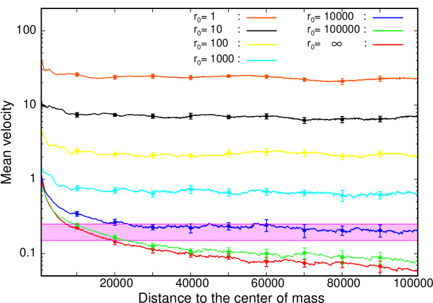
Figure 4: The MOGA ($log-$) rotation velocities of the objects in the galaxy models of the Milky Way as a function of the distances to their center of mass in the galaxies and for various values of the distance $r_{0}$ for the onset of the inverse attraction. Distance is in parsec and the velocities are in MD units where a mean velocity $\bar{v}\approx 0.15-0.25$ corresponds $\bar{v}=220$ km s^-1 in the Milky Way. The velocity interval in magenta is for velocities that correspond to rotation velocities $v\in[0.15,0.25]$.

The rotation velocity of stars in the Milky Way can be related to the rotation velocities in the MOGA models of a galaxy. The relation between lengths is obtained from the sizes of the galaxies, and the relation between velocities is obtained from the rotation time and velocity in the Milky Way and the corresponding rotation time and velocities in the models of galaxies. The rotation velocity of stars in the Milky Way at the distances $r\in[6.72,8.40]$ kpc is $v(r)=220\pm 10$ km s^-1 Camarillo2018 . An estimate of the mean velocity of the objects in the models for a galaxy is associated with uncertainty. The mean rotation velocity $\bar{v}\approx 0.15-0.25$ in the galaxy models is determined to correspond to the mean rotation velocity $v=220$ km s^-1 in the Milky Way Toxvaerd2022a , and the colored area in Figure 4 is for mean rotation velocities in the interval $v\in[0.15,0.25]$. The IA attractions increase systematically the mean velocities of the baryonic objects, and the rotation velocities in the MOGA galaxies only agree with the observed velocities in the Milky Way for a large value of the modification distance $r_{0}$. The simulations indicate that the stability of a galaxy with a rather constant rotation velocity which corresponds to $\approx$ the rotation velocity in the Milky Way can be obtained by a modification of the attractions for far away objects with distances corresponding to $r\geq 10$ kpc (blue curve in Figure 4). The estimation is with a big uncertainty, but one can, however, exclude a significantly shorter value of the modification range $r_{0}$. A smaller value than $r_{0}$= 10 kpc will according to the results in Figure 4 lead to an unrealistic high rotation velocity. The enhanced accelerations (MOND) or attractions (MOGA) for $r_{0}\leq 1000\rightarrow a_{0}\geq 1.0\times 10^{-6}$ result in a too high mean rotation velocity for MOGA, and in the case of MOND, the galaxy is spontaneously destabilized.

IV Conclusion

The modification of the gravitational attraction from a Newtonian ISL attraction to an IA attraction for pairs of baryonic objects at distances $r\geq r_{0}$ stabilizes the objects in the galaxy (Figure 2). Furthermore, it changes the mean rotation velocity of objects in the galaxy from a classical Newtonian/Kepler behavior to a rather constant velocity with respect to the distance to the center of rotation in the galaxy (Figure 4). The rotation velocity in the galaxies with MOGA is in qualitative agreement with the observed rotation velocity in the Milky Way and in galaxies in the Universe Corbelli2000 ; Gentile2011 ; Camarillo2018 . The Hubble expansion results in that the MOGA galaxies occasionally lose a bound object, whereas the galaxies with the corresponding MOND dynamics are unstable.

A galaxy and the Milky Way contain hundreds of billions of stars and a substantial amount of baryonic gas Gupta2012 ; Bergma2018 , and it is not possible to determine the exact discrete dynamics for MOND or MOGA for a system with this number of objects. The question is if one can extrapolate the qualitative behavior of the exact dynamics for a system of only a few hundred bound objects in rotations around their mass center to the behavior of a baryonic system of hundreds of billions of stars. And if so, what can then explain the change of the gravitational attraction from a Newtonian ISL attraction to an IA attraction? Modifications of the Newtonian ISL to an IA-like attraction have been proposed for a long time in an attempt to obtain the stability of galaxies by the standard model Fischbach2001 ; Adelberger2003 ; Henrichs2021 . Here I would like to propose another possibility, viz gravitational lensing Bartelmann2010 ; Abbott2016 ; Mukherjee2021 and focusing, caused by heavy centers of mass in the galaxy of the gravitational waves from objects in the galaxy that are located at long distances from the object.

Appendix A The discrete algorithm

The classical mechanical simulations of the dynamics of interacting objects are performed by using Newton’s algorithm for discrete classical dynamics Newton1687 . Simulations of molecular and atomic systems are named ”Molecular Dynamics” (MD), and almost all MD simulations and many simulations in celestial mechanics are performed using Newton’s algorithm, but with the name ”Leap-frog” or the ”Verlet algorithm” Verlet1967 , and the algorithm also appears under a variety of other names. It was, however, Isaac Newton who first formulated the Discrete Molecular Dynamics algorithm, when he in PHILOSOPHIÆ NATURALIS PRINCIPIA MATHEMATICA $(Principia)$ derived his second law for classical mechanics Newton1687 ; Toxvaerd2020 ; Toxvaerd2023 .

A.1 Newton’s Discrete Molecular Dynamics algorithm

In Newton’s discrete dynamics a new position $\textbf{r}_{i}(t+\delta t)$ at time $t+\delta t$ of an object $i$ with the mass $m_{i}$ is determined by the force $\textbf{f}_{i}(t)$ acting on the object at the discrete positions $\textbf{r}_{i}(t)$ at time $t$, and the position $\textbf{r}_{i}(t-\delta t)$ at $t-\delta t$ as

$$m_{i}\frac{\textbf{r}_{i}(t+\delta t)-\textbf{r}_{i}(t)}{\delta t}=m_{i}\frac{\textbf{r}_{i}(t)-\textbf{r}_{i}(t-\delta t)}{\delta t}+\delta t\textbf{f}_{i}(t),$$ (14)

where the momenta $\textbf{p}_{i}(t+\delta t/2)=m_{i}(\textbf{r}_{i}(t+\delta t)-\textbf{r}_{i}(t))/\delta t$ and $\textbf{p}_{i}(t-\delta t/2)=m_{i}(\textbf{r}_{i}(t)-\textbf{r}_{i}(t-\delta t))/\delta t$ are constant in the time intervals in between the discrete positions. Newton begins Principia by postulating Eq. (A.1) in Proposition I, and he obtained his second law as the limit $lim_{\delta t\rightarrow 0}$ of the equation.

Usually, the algorithm, Eq. (A.1), is presented as the Leap-frog algorithm for the velocities

$$\textbf{v}_{i}(t+\delta t/2)=\textbf{v}_{i}(t-\delta t/2)+\delta t/m_{i}\textbf{f}_{i}(t),$$ (15)

and the positions are determined from the discrete values of the momenta/velocities as

$$\textbf{r}_{i}(t+\delta t)=\textbf{r}_{i}(t)+\delta t\textbf{v}_{i}(t+\delta t/2).$$ (16)

The rearrangement of Eq. (A.1) gives the Verlet algorithm Verlet1967

$$\textbf{r}_{i}(t+\delta t)=2\textbf{r}_{i}(t)-\textbf{r}_{i}(t-\delta t)+\delta t\textbf{f}_{i}(t)^{2}/m_{i}.$$ (17)

A.2 The invariances in Classical Mechanics, Discrete Molecular Dynamics, MOND and MOGA

Classical analytic dynamics are time-reversible and symplectic and a conservative system of $N$ baryonic objects has three invariances: conserved momentum, angular momentum, and energy. Newton’s discrete Molecular Dynamics is also reversible and symplectic and has the same invariances. MOGA and MOND are time-reversible and symplectic, but only MOGA maintains the three invariances, whereas MOND does not ensure momentum and angular momentum conservation. The proof is given below.

Newton’s discrete dynamics for a system of $N$ spherically symmetrical objects with masses $m^{N}\equiv m_{1},m_{2},..,m_{i},..,m_{N}$ and positions r${}^{N}(t)\equiv$ r${}_{1}(t)$, r${}_{2}(t),..,$r${}_{i}(t),..$r${}_{N}(t)$ is obtained by Eqn. (A.1). Let the force, $\textbf{F}_{i}$ on object No $i$ be a sum of pairwise forces $\textbf{f}_{ij}$ between pairs of objects $i$ and $j$

$$\textbf{F}_{i}=\sum_{j\neq i}^{N}\textbf{f}_{ij}.$$ (18)

Newton’s discrete dynamics, Eq. (A.1) is a central difference algorithm and it is time symmetrical, so the discrete dynamics is time reversible and symplectic Friedman1991 . MOND and MOGA with Eq. (A.1) are also time reversible and symplectic.

The momentum for a conservative system with the discrete dynamics, Eq. (A.1) of the $N$ objects is conserved since

$$\sum_{i}^{N}m_{i}\frac{\textbf{r}_{i}(t+\delta t/2)-\textbf{r}_{i}(t)}{\delta t}=\sum_{i}^{N}\textbf{p}_{i}(t+\delta t/2)=$$ (19)

$$\sum_{i}^{N}\textbf{p}_{i}(t-\delta t/2)+\delta t\sum_{i,j\neq i}^{N}\textbf{f}_{ij}(t)=\sum_{i}^{N}\textbf{p}_{i}(t-\delta t/2),$$

where $\sum_{i,j\neq i}^{N}\textbf{f}_{ij}(t)=0$ with $\textbf{f}_{ij}(t)=-\textbf{f}_{ji}(t)$ due to Newton’s third law. But only the discrete dynamics and MOGA conserve the momentum, whereas MOND does not because (see Eq. (7)) Felten1984

$$\textbf{f}_{ij}(t)\sqrt{1+4m_{i}a_{0}/\mid F_{i}\mid}\neq-\textbf{f}_{ji}(t)\sqrt{1+4m_{j}a_{0}/\mid F_{j}\mid}.$$ (20)

The shortcoming of MOND with respect to momentum conservation is independent of the algorithm because the momentum conservation in analytic dynamics is also ensured by $\sum_{i,j\neq i}^{N}\textbf{f}_{ij}(t)=0$.

The discrete positions and momenta are not known simultaneously. An expression for the angular momentum of the conservative system is

$$\textbf{L}(t)=\sum_{i}^{N}\textbf{r}_{i}(t)\times(\textbf{p}_{i}(t+\delta t/2)+\textbf{p}_{i}(t-\delta t/2))/2$$

$$=\sum_{i}^{N}\textbf{r}_{i}(t)\times(m_{i}\textbf{r}_{i}(t+\delta t)-m_{i}\textbf{r}_{i}(t-\delta t))/2\delta t).$$ (21)

The angular momentum is conserved since (using $\textbf{r}_{i}(t)\times(\textbf{f}_{ij}(t)+\textbf{f}_{ji}(t))=0,$ $\textbf{a}\times\textbf{a}=0,$ $\textbf{a}\times\textbf{b}=-\textbf{b}\times\textbf{a}$ and Eq. (A.4) )

$$2\delta t\textbf{L}(t)=\sum_{i}^{N}\textbf{r}_{i}(t)\times(m_{i}\textbf{r}_{i}(t+\delta t)-m_{i}\textbf{r}_{i}(t-\delta t))$$

$$=\sum_{i}^{N}m_{i}\textbf{r}_{i}(t)\times(2\textbf{r}_{i}(t)-2\textbf{r}_{i}(t-\delta t))=\sum_{i}^{N}m_{i}\textbf{r}_{i}(t-\delta t)\times(\textbf{r}_{i}(t)+\textbf{r}_{i}(t))$$

$$=\sum_{i}^{N}m_{i}\textbf{r}_{i}(t-\delta t)\times(\textbf{r}_{i}(t)-\textbf{r}_{i}(t-2\delta t))=2\delta t\textbf{L}(t-\delta t).$$ (22)

MOGA fulfils Newton’s third law with $\sum_{i,j\neq i}^{N}\textbf{f}_{ij}(t)=0$ and conserves the angular moment whereas MOND does not conserve this invariance.

The energy in analytic dynamics is the sum of potential energy $U(\textbf{r}^{N}(t))$ and kinetic energy $K(t)$, and it is an invariance for a conservative system. The kinetic energy at time $t$ in the discrete dynamics is, however, ill-defined since the velocities change at time $t$. The energy invariance in the discrete dynamics can, however, be seen by considering the change in kinetic energy, $\delta K([t-\delta t/2,t+\delta t/2])$ and potential energy and $\delta U([t-\delta t/2,t+\delta t/2])$ in the time interval $[t-\delta t/2,t+\delta t/2]$.

The loss in potential energy, $-\delta U$ is defined as the work done by the forces at a move of the positions Goldstein . An expression for the work, $W$ done in the time interval by the discrete dynamics from the position $(\textbf{r}_{i}(t)+(\textbf{r}_{i}(t-\delta t))/2$ at $t-\delta t/2$ to the position $(\textbf{r}_{i}(t+\delta t)+\textbf{r}_{i}(t))/2$ at $t+\delta t/2$ is Toxvaerd2023

$$-\delta U=W=\sum_{i}^{N}\textbf{f}_{i}(t)(\frac{\textbf{r}_{i}(t+\delta t)+\textbf{r}_{i}(t)}{2}-\frac{\textbf{r}_{i}(t)+\textbf{r}_{i}(t-\delta t)}{2})$$ (23)

$$=-\sum_{i}^{N}\textbf{f}_{i}(t)(\textbf{r}_{i}(t+\delta t)-\textbf{r}_{i}(t-\delta t))/2.$$

By rewriting Eq. (A.4) to

$$\textbf{r}_{i}(t+\delta t)-\textbf{r}_{i}(t-\delta t)=2(\textbf{r}_{i}(t)-\textbf{r}_{i}(t-\delta t))+\frac{\delta t^{2}}{m_{i}}\textbf{f}_{i}(t),$$ (24)

and inserting in Eq. (A.10) one obtains an expression for the total work in the time interval

$$-\delta U=W=\sum_{i}^{N}[(\textbf{r}_{i}(t)-\textbf{r}_{i}(t-\delta t))\textbf{f}_{i}(t)+\frac{\delta t^{2}}{2m_{i}}\textbf{f}_{i}(t)^{2}].$$ (25)

The change in kinetic energy in the time interval $[t-\delta t/2,t+\delta t/2]$ is

$$\delta K=\sum_{i}^{N}\frac{1}{2}m_{i}[\frac{(\frac{\textbf{r}_{i}(t+\delta t)+\textbf{r}_{i}(t)}{2}-\textbf{r}_{i}(t))^{2}}{(\delta t/2)^{2}}-\frac{(\textbf{r}_{i}(t)-\frac{\textbf{r}_{i}(t)+\textbf{r}_{i}(t-\delta t)}{2})^{2}}{(\delta t/2)^{2}}]$$ (26)

$$=\sum_{i}^{N}\frac{1}{2}m_{i}[\frac{(\textbf{r}_{i}(t+\delta t)-\textbf{r}_{i}(t))^{2}}{\delta t^{2}}-\frac{(\textbf{r}_{i}(t)-\textbf{r}_{i}(t-\delta t))^{2}}{\delta t^{2}}].$$

By rewriting Eq. (A.4) to

$$\textbf{r}_{i}(t+\delta t)-\textbf{r}_{i}(t)=\textbf{r}_{i}(t)-\textbf{r}_{i}(t-\delta t)+\frac{\delta t^{2}}{m_{i}}\textbf{f}_{i}(t)$$ (27)

and inserting the squared expression for $\textbf{r}_{i}(t+\delta t)-\textbf{r}_{i}(t)$ in Eq. (A.13), the change in kinetic energy is

$$\delta K=\sum_{i}^{N}[(\textbf{r}_{i}(t)-\textbf{r}_{i}(t-\delta t))\textbf{f}_{i}(t)+\frac{\delta t^{2}}{2m_{i}}\textbf{f}_{i}(t)^{2}].$$ (28)

The energy invariance in Newton’s discrete dynamics is expressed by Eqn. (A.12), and Eq. (A.15) as Toxvaerd2023

$$\delta E=\delta U+\delta K=0.$$ (29)

The energy invariance is due to the time symmetry, and it is valid for any discrete force. It does not rely on the existence of an analytic force with an analytic potential.

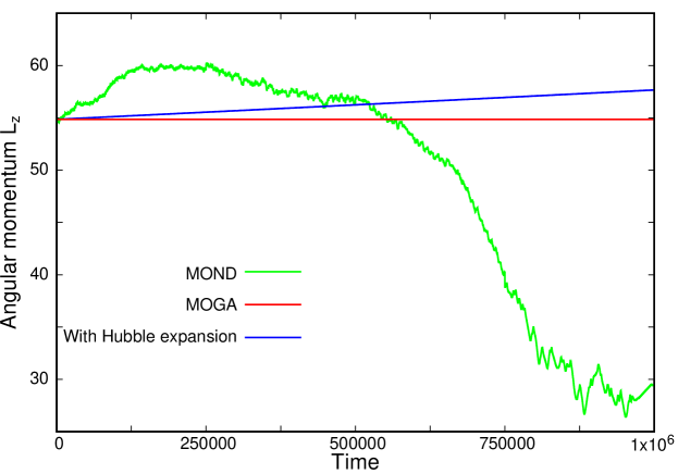
Figure 5: Time evolution of the z-component, $\textrm{L}_{z}$, of the angular momentum of the galaxies. In green is $\textrm{L}_{z}$ for MOND with $a_{0}=10^{-10}$. The red line is the conserved $\textrm{L}_{z}$ for the Newtonian and MOGA dynamics without a Hubble expansion. The corresponding evolution of $\textrm{L}_{z}$ with the Hubble expansion included is shown in blue.

A.3 The simulations with Discrete Molecular Dynamics, MOND and MOGA

The simulations are started with various start configurations of positions $\textbf{r}(0)^{N}$ and with the small time increment $\delta t=0.0025$. Each simulations are performed for $3.2\times 10^{9}$ time steps corresponding to a reduced time $t=8.0\times 10^{6}\approx$ 13.4 Gyr Toxvaerd2022 . The exact algorithm is absolutely stable and all the simulations are performed without any constraints or adjustments. The algorithm and the explanation of the stability of Newton’s discrete algorithm are explained in a recent review of Discrete Molecular Dynamics Toxvaerd2023 .

MOND is simulated with the modified acceleration, Eq. (7), and MOGA with the modified forces, Eq.(10). All the simulations conserve energy, Newtonian dynamics, and MOGA conserve also momentum and angular momentum, but MOND does not. Figure A1 shows the time evolution for $4.\times 10^{8}$ time-steps in green of the z-component of the angular momentum with MOND dynamics for the galaxies shown in the previous figures, together with the corresponding components with pure Newtonian or MOGA dynamics and without Hubble expansion in red, and with the Hubble expansion in blue. The simulations are started with a disk-like configuration $\textbf{r}(0)^{N}$ with $\textrm{L}_{x}\approx 0$ and $\textrm{L}_{y}\approx 0$ and with $\textrm{L}_{z}=54.85$. The simulation with MOND in green is for the small value $a_{0}=10^{-10}$ with the number of objects in the galaxy shown in green in Figure 2. The momentum and the angular momentum with MOND vary with time, whereas the momentum and angular momentum with Newtonian dynamics and with MOGA without the Hubble expansion is conserved. The Hubble expansion and with Newtonian dynamics or with MOGA (blue line) increases the angular momentum monotonically, but very slowly. The MOND angular momentum shown in Figure A1 is for $a_{0}=10^{-10}$. The values of the angular momentum for larger values of $a_{0}$ fluctuate with amplitudes that are decades bigger and the objects are released from the galaxy (Figure 2).


Acknowledgements This work was supported by the VILLUM Foundation Matter project, grant No. 16515.

Data Availability Statement Data will be available on request.

References

- (1) J. G. de Swart, G. Bertone and J.van Dongen, Nat. Astron., 1 0059 (2017).
- (2) J. S. Bullock and M. Boylan-Kolchin, Annu. Rev. Astron. Astrophys., 55 343 (2017).
- (3) L. Perivolaropoulos and F. Skara, New Astron. Rev., 95 101659 (2022).
- (4) E. Fischbach, D. E. Krause, V. M. Mostepanenko and M. Novello, Phys. Rev. D, 64 075010 (2001).
- (5) E. G. Adelberger, B. R. Heckel and A. E. Nelson, Annu. Re. Nucl. Part. Sci., 53 77 (2003).
- (6) J. G. Lee, E. G. Adelberger, T. S. Cook, S. M. Fleischer and B. R. Heckel, Phys. Rev. Lett., 124 101101 (2020).
- (7) J. Henrichs, M. Lembo, F. Iocco and L. Amendola, Phys. Rev. D, 104 043009 (2021).
- (8) V. C. Rubin, W. K. Ford Jr. and N. Thonnard, Astrophys. J., 238 471 (1980).
- (9) V. C. Rubin, D. Burstein, W. K. Ford Jr. and N. Thonnard N 1985 Astrophys. J. 289 81 (1985).
- (10) G .Gentile, B. Famaey and W. J. G. de Blok, A&A, 527 A76 (2011).
- (11) E. Corbelli and P. Salucci, Mon. Not. R. Astron. Soc., 311 441 (2000).
- (12) G. Bertone, D. Hooper, Rev. Mod. Phys., 90 045002 (2018).
- (13) M. Milgrom, Apj, 270 371 (1983).
- (14) J. D. Berkenstein and M. Milgrom, Astrophys. J., 286 7 (1984).
- (15) B. Famaey and S. McGaugh, Living Rev. Relativity, 15 10 (2012).
- (16) T. Clifton, P. G. Ferreira, A. Padilla and C.Skordis, Phys. Rep., 5 (2012).
- (17) S. Mendoza, Can. J. Phys., 93 217 (2015).
- (18) M. Bartelmann, Clas. Quantum Grav., 27 233001 (2010).
- (19) S.Mukherjee, B. D. Wandelt, S. M. Nissanke and A. Silvestri, Phys. Rev. D, 103 043520 (2021).
- (20) B. P. Abbott et al., Phys. Rev. Lett., 116 061102 (2016).
- (21) S. Boran, S. Desai, E. O. Kahya and R. P. Woodard, Phys. Rev. D, 97 041501(R) (2018).
- (22) R. W. Hockney, S. P. Goel and J. W. Eastwood, J. Comput. Phys., 14 148 (1974).
- (23) A. A. Klypin and S. F. Shandarin, MNRAS, 204 891 (1983).
- (24) J. Centrella and A. L. Melott, Nature, 305 196 (1983).
- (25) Ya. B. Zeldovich, Astrom. & Astrophys., 5 84 (1970).
- (26) V. Springel, MNRAS, 364 1105 (2005).
- (27) D. J. Price et al, Publ. Astron. Soc. Aust., 35 e031 (2018).
- (28) R. Weinberger, V.Springel and R. Pakmor, Astrophys. J., Suppl. Ser., 248 :32 (2020).
- (29) J. Schaye et al., MNRAS, 402 1536 (2010).
- (30) Y. Dubois, M.Volonteri and J. Silk, MNRAS, 440 1590 (2014).
- (31) M. Vogelsberger et al., MNRAS, 444 1518 (2014).
- (32) Y. Dubois et al., MNRAS, 463 3948 (2016).
- (33) A. D. Ludlow, S. M. Fall, J.Schaye and D. Obreschkow, MNRAS, 508 5114 (2021).
- (34) G. W. Angus, G. Gentile, A. Diaferio, B. Famaey and K.J. van der Heyden, MNRAS, 440 746 (2014).
- (35) G. W. Angus, A. Diaferio, B. Famaey and K.J. van der Heyden, J. Astrophys. Astron., 10 079 (2014).
- (36) F. Lüghausen, B. Famaey and P Kroupa, MNRAS, 441 2497 (2014).
- (37) M. Vogelsberger, F. Marinacci, P.Torrey and E. Puchwein, Nat. Rev. Phys, 2 42 (2020).
- (38) I. Newton , PHILOSOPHIÆ NATURALIS PRINCIPIA MATHEMATICA. LONDINI, Anno MDCLXXXVII. Second Ed.1713; Third Ed. (1726)
- (39) S. Toxvaerd, Eur. Phys. J. Plus, 135 267 (2020).
- (40) S. Toxvaerd, Eur. Phys. J. Phys., 137 :99 (2022).
- (41) S. Toxvaerd, Class. Quantum Grav., 29 22500 (2022).
- (42) S. Toxvaerd, Comprehensive Computational Chemistry, 3 329 (2023).
- (43) J. E. Felten, Astron. J., 286 3 (1984).
- (44) Y-J. Chen, W. K. Tham, D. E. Krause, D. López, E. Fischback and R. S. Decca, Phys. Rev. Lett., 116 221102 (2016).
- (45) G. Bimonte, B. Spreng, P. A. Maia Neto, G-L. Ingold, G. L. Klimchitskaya, V. M. Mostepanenko and R. S. Decca, Universe, 7 93 (2021).
- (46) J. Baeza-Ballesteros, A. Donini and S. Nadal-Gisbert, Eur. Phys. J. C, 82: 154 (2022).
- (47) H-W. Rix and J. Bovy, Astron. Astrophys. Rev., 21 61 (2013).
- (48) A. J. Daeson et al., MNRAS, 496 3929 (2020).
- (49) Z-Z. Li and J. Han, Astrophys. J. Lett., 915 L18 (2021).
- (50) S. J. Aerseth, MNRAS, 126 223 (1963).
- (51) A. Gupta, S. Mathur, Y. Krongold, F. Nicastro and M. Galeazzi, Astrophys. J. Lett., 756 :L8 (2012).
- (52) J. N. Bergma, M. E. Anderson, M. J. Miller, E. Hodges-Kluck, X. Dai, J-T. Li, Y. Li and Z. Qu, Astrophys. J., 862 :3 (2018).
- (53) J. Soltis, S. Casertano and A. G. Riess, Astrophys. J. Lett., 908 L5 (2021).
- (54) B. Famaey and J. Binney, MNRAS, 363 603 (2005).
- (55) T. Camarillo, P. Dredger and B. Ratra, Astrophys. Space Sci., 363 :268 (2018).
- (56) L. Verlet, Phys. Rev., 159, 98 (1967).
- (57) A. Friedman and S. P. J. Auerbach S P J, J. Comput. Phys., 93 177, 93 189 (1991).
- (58) H. Goldstein, Classical Mechanics, (Addison-Wesley Press Second Ed. 1980), Chap. 1.