OORD: The Oxford Offroad Radar Dataset

Abstract

There is a growing academic interest as well as commercial exploitation of millimetre-wave scanning radar for autonomous vehicle localisation and scene understanding. Although several datasets to support this research area have been released, they are primarily focused on urban or semi-urban environments. Nevertheless, rugged offroad deployments are important application areas which also present unique challenges and opportunities for this sensor technology. Therefore, the Oxford Offroad Radar Dataset (OORD) presents data collected in the rugged Scottish highlands in extreme weather. The radar data we offer to the community are accompanied by GPS/INS reference – to further stimulate research in radar place recognition. In total we release over $90\text{\,}\mathrm{GiB}$ of radar scans as well as GPS and IMU readings by driving a diverse set of four routes over $11$ forays, totalling approximately $154\text{\,}\mathrm{km}$ of rugged driving. This is an area increasingly explored in literature, and we therefore present and release examples of recent open-sourced radar place recognition systems and their performance on our dataset. This includes a learned neural network, the weights of which we also release. The data and tools are made freely available to the community at oxford-robotics-institute.github.io/oord-dataset

Figure 1: Our data collection site is in the Scottish Highlands, with comprehensive coverage of Ardverikie Estate, close to the historic boundary between Lochaber and Badenoch. This image is taken on Lochan na h-Earba from our LABEL:DA1 and LABEL:DA2 datasets (Secs. III-D and III-E), showing unpaved terrain over, uneven landscape next to the vehicle, and the inclement weather. Images, GPS traces, and example radar scans for more specific areas of Ardverikie Estate are provided in Figs. 3 and 8.

I Introduction

Compared to cameras and LiDARs, radar systems offer distinct advantages, including extended-range perception and resilience to lightning and various weather conditions. Full reviews of millimetre-wave radar applications in autonomous vehicle tasks are available in e.g. [1, 2]. In brief, scanning radar-based motion estimation [3, 4, 5, 6, 7, 8, 9, 10], pose estimation [11, 12, 13], place recognition [14, 15, 11, 16, 17, 18, 19, 20, 21, 22, 23], and full simultaneous localisation and mapping (SLAM) [24, 25] are increasingly popular in the literature. This dataset is designed to support that work, and to prompt an extension into naturalistic, rugged environments, which have not yet been explored.

Natural environments are important because off-road autonomous vehicles have many essential applications across industries operating on rugged terrain. This technology is essential for tasks such as agricultural operations, search and rescue missions, and exploration in remote areas, where human intervention may be impractical or hazardous. Also, autonomous hauling or resource extraction is important in mining, autonomous tractors for planting and harvesting can optimise crop yields, tree planting and logging can reduce environmental impact and risk to workers, autonomous grading and excavation can enhance efficiency and safety in construction, search and rescue missions can leverage autonomous drones to locate missing persons in hazardous locations, and autonomous vehicles can be of great use in environmental monitoring and disaster response.

In deploying autonomous machines to these sites, place recognition is vital for navigation and localisation. For this, more robust sensors are crucial to enhancing place recognition accuracy and reliability. Radar in particular can handle challenging conditions like low-light environments.

We therefore present an offroad radar dataset with a focus on relocalisation, with Fig. 1 showing an example location from our collection site. Our contributions are as follows:

1. Offroad scanning radar data We release the first radar dataset focusing on off-road, difficult terrain and naturalistic environments,

2. Poor weather and lighthing conditions including collection after thick snowfall and in total darkness (being in the wilderness),

3. Place recognition ground truth Our raw data is referenced against good GPS as a ground truth for the place recognition task,

4. Open-sourced radar place recognition implementations For the first time, we release open-source a set of trained weights for a deep neural network which solves the radar place recognition,

5. Software development kit We release software tools for making the use of this dataset in some pre-existing, non-learned open-source radar place recognition implementations easy, as well as pipelines to accelerate new learning solutions.

In Sec. III we describe and justify the choice of collection sites. Sec. IV describes the data collection platform, sensor format including radar as well as the GPS/INS synchronised with this main sensor, and the download data structure for how to interact with the dataset. Sec. V presents several useful software tools which make it easy to apply this data, e.g. with common performance metrics and data formats. Finally, Sec. VI shows examples based off of the tools in Sec. V for several publicly available place recognition algorithms as tested against this dataset.

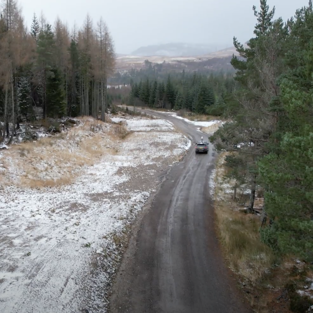
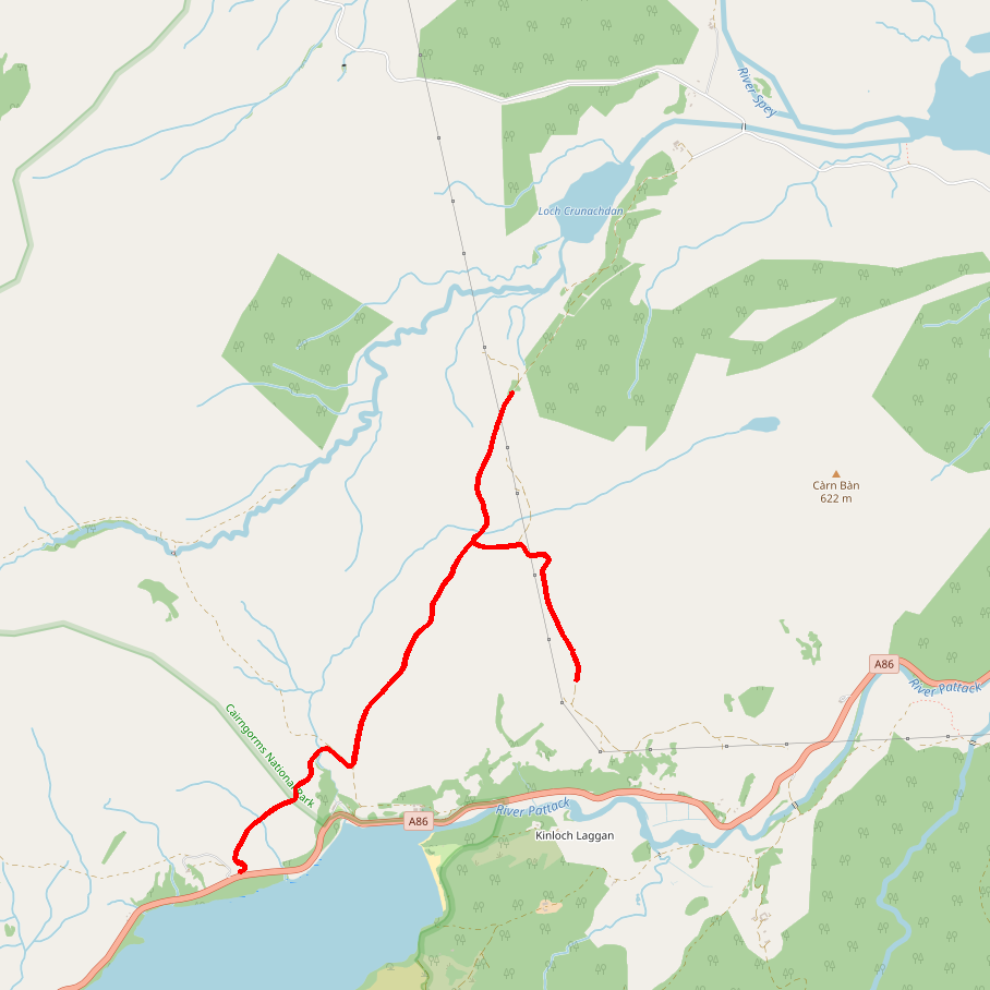
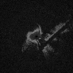
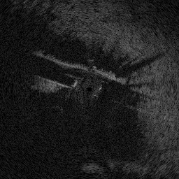
(a) The bellmouth dataset is on gravel tracks ascending and descending a mountail tail, with the descent along the same path but in the opposite direction.

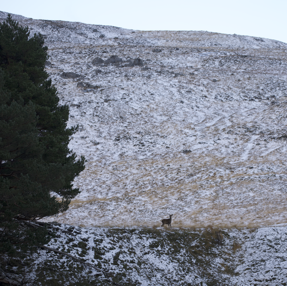
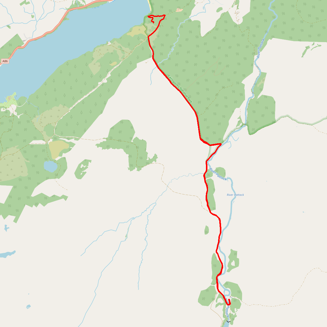
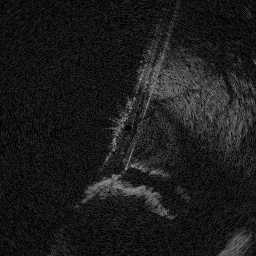
(b) The hydro dataset ascends to the highest elevation of all of our routes, and descends along the same track. Much of the route is along the River Pattack.

Figure 3: The twolochs and bellmouth datasets, with GPS traces, trajectory-to-trajectory ground truth GPS matrices, and some sample radar scans.

Dataset	Variable terrain	Poor weather	Scene diversity	Repeat traversals
Radar RobotCar	✗	✗	✗	✓
Marulan	✓	✓	✓	✓
MulRan	✗	✗	✓	✓
RADIATE	✗	✓	✓	✗
Boreas	✗	✓	✓	✓
OSDaR23	✗	✗	✓	✗
OORD (Ours)	✓	✓	✓	✓

TABLE I: Comparison of features of our dataset in comparison to other radar datasets in literature. Marulan is closest in characteristics to ours, but is collected with a short-range sensor, $40\text{\,}\mathrm{m}$ as opposed to our $165\text{\,}\mathrm{m}$ range.

II Related Work

II-A Radar datasets

Datasets featuring a similar class of millimetre-wave scanning radar include Marulan [26] by Peynot et al, which is furthermore also collected in natural environments, as is ours. This data, however, only has range of up to $40\text{\,}\mathrm{m}$. Several recent radar datasets use the same radar class – from the same manufacturer – as used in our work, including the Oxford Radar RobotCar Dataset [27] by Barnes et al, MulRan [14] by Kim et al, RADIATE [28] by Sheeny et al, Boreas [29] by Burnett et al, and OSDaR23 [30] by Tagiew et al. The Oxford Radar RobotCar Dataset [27] is purely urban and features many repeat traversals, useful in investigating place recognition. The ground truth provided in [27], however, is prepared for radar odometry rather than place recognition. MulRan [14] presents more diversity in scenery, having been collected in several distinct parts of Daejeon, South Korea. We similarly attend to generalisation-sensitive training/testing data and collect at many sites, albeit offroad and more widespread across a country rather than a city. Our repeat traversals are also more numerous than for MulRan. RADIATE [28], presenting vehicle detection and tracking ground truth, is similarly lacking in overlapping traversals and not geared towards place recognition, although a diversity in weather makes this dataset interesting for exploring this sensor’s robustness. Closest to our work is Boreas by Burnett et al [29], who collect multi-season data including a Navtech CIR304-H scanning radar. Our work is in part inspired by this, with ours featuring highly non-planar offroad driving as opposed to purely urban.

Tab. I summarises the characteristics of our dataset as compared to these.

II-B Radar place recognition

Owing to its inherent resilience in sensing capabilities, radar has attracted considerable attention for its adeptness in the face of adverse weather, demonstrating a capacity to navigate and operate effectively in inclement conditions. This is because radar systems typically use electromagnetic waves in the radio or microwave frequency range. Unlike visible light, these waves can penetrate through various weather elements like rain, snow, fog, and clouds without significant distortion or attenuation. Radar place recognition has thus been explored in [15, 11, 31, 16, 18, 19, 32, 33, 34, 23].

This has included simultaneous localisation and mapping [32, 33] with loop closure detection mechanisms, where for example in [32] loop candidates are rejected by principal components analysis to focus on distinct structural layouts.

There are also several methods for learning to vectorise radar scans with neural networks  [15, 11, 19, 16, 18, 23], including supervised [15, 11, 16, 16] and self-supervised approaches [23, 19] and learned uncertainty [23].

Finally, some approaches are non-learned [14, 31, 34, 35], instead relying largely on transformation-vinvariant integral transforms (e.g. Fourier, Fourier-Mellin, Radon) as in [34, 35], pooling operations such as max/min/mean to achieve rotation invariance and to reduce the representation dimensionality [14, 35], and circular cross-correlation for an alignment/similarity score [14, 34].

This area is therefore of increasing interest, but far from mature, and this dataset should therefore contribute to establishing useful benchmarks for the community.

III Off-road routes & collection sites

Route	Distance	# Radar	# GPS	Size
Bellmouth $\times 4$	$8.98\text{\,}\mathrm{km}$	$7781$	$7091$	$6.65\text{\,}\mathrm{GiB}$
Hydro $\times 3$	$13.65\text{\,}\mathrm{km}$	$11094$	$11054$	$8.93\text{\,}\mathrm{GiB}$
Maree $\times 2$	$16.87\text{\,}\mathrm{km}$	$11462$	$11427$	$9.05\text{\,}\mathrm{GiB}$
Two Lochs $\times 2$	$20.62\text{\,}\mathrm{km}$	$14938$	$14922$	$11.70\text{\,}\mathrm{GiB}$

TABLE II: Summary statistics for the various routes to the sites they represent. Quantities in each row are from an example foray on that route – the total distance driven in our dataset is approximately $154\text{\,}\mathrm{km}$ and approximately $90\text{\,}\mathrm{GiB}$.

Figs. 3 and 8 show a detailed overview of the datasets we provide, at various areas of the Ardverikie Estate. Data has been gathered in the region encompassing Loch Laggan and Lochan na h-Earba. The position of these lochs can be particularly well understood by referring to the caption of Fig. 8(b).

Loch Laggan, a freshwater loch located about $10\text{\,}\mathrm{km}$ west of Dalwhinnie in the Scottish Highlands, extends in a nearly northeast to southwest direction for approximately $11\text{\,}\mathrm{km}$. The name Lochan na h-Earba actually refers to two lochs positioned south of Loch Laggan. These lochs are situated in a slender glen that runs from southwest to northeast, running roughly parallel to Loch Laggan. The Binnein Shuas range of hills separates them from Loch Laggan.

Each of Figs. 8(b), 3(a), 8(a) and 3(b) is arranged as follows: Top Left: Photograph of each dataset collection location (handheld camera, not on-board imagery). Top Middle: GPS trace of route driven. Top Right: Ground truth match matrix for a pair of trajectories at that site. Bottom: Example radar scans from various points along the route (Cartesian).

We release data from four areas of the Ardverikie Estate. These feature distinct landscape (therefore typical radar returns) as well as driving conditions. We refer to the sites as Two Lochs, Bellmouth, Maree, and Hydro. Each of these is discussed below. Tab. II summarises the collection sites and routes. Fig. 4 compares the elevation along each route.

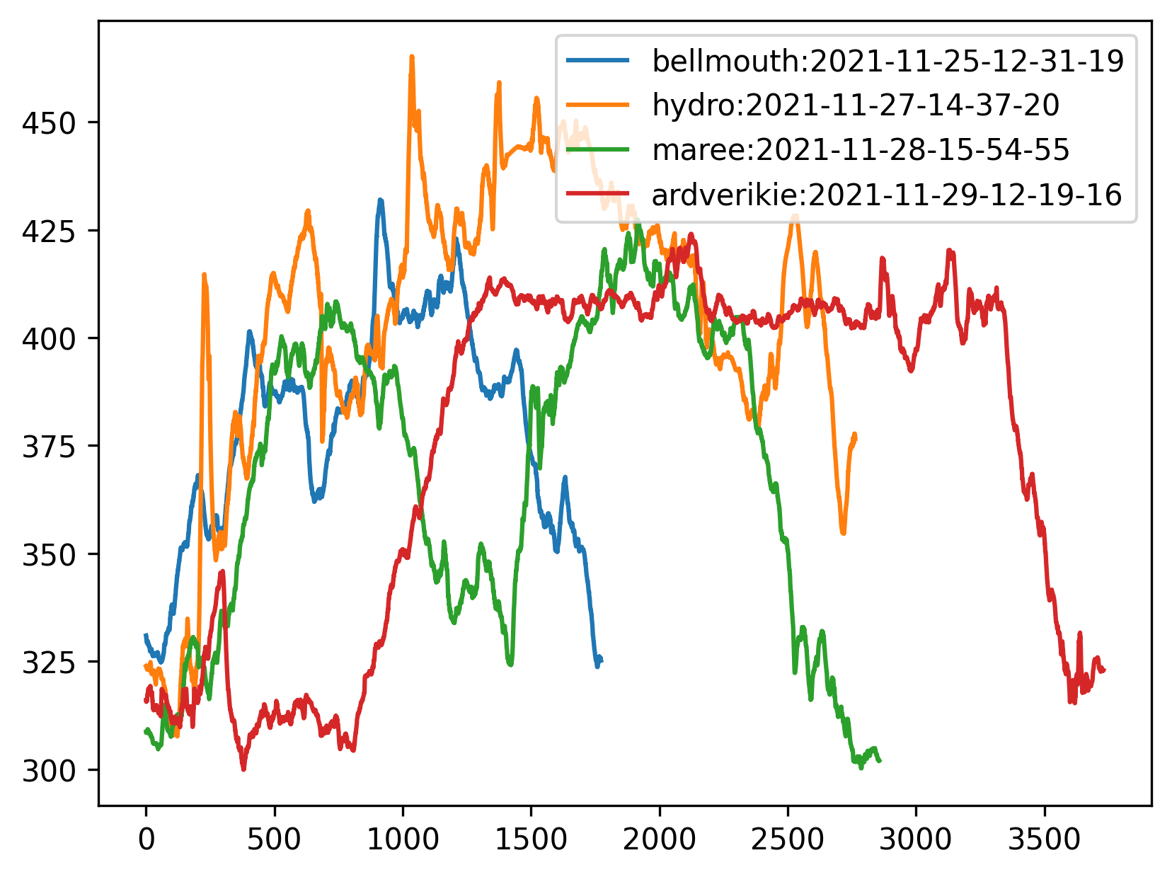
Figure 4: Changes in elevation (measured as UTM down) for example forays from each challenge site.

III-A Route 1: Bellmouth

This is a $8.98\text{\,}\mathrm{km}$ route. The route is completely landlocked, heading away from and then back towards Loch Laggan, see Fig. 3(a) (Top Middle. The ascent and descent are reflected by a somewhat symmetrical elevation change in Fig. 4 – climbing for the first half of the route, and descending for the second half. The vehicle is always on a gravel track. Figs. 5(b), 5(a), 5(d) and 5(c) show images from the vehicle’s perspective from four outings along this route. The first two these outings is prior to any snow falling in the Ardverikie Estate area (Figs. 5(a) and 5(b)). The next two of these outings show significant snow dump (Figs. 5(c) and 5(d)). The outings are in the same direction, as per the ground truth matrix in Fig. 8(b) (Top Right), but within each outing itself we double back (c.f. the off diagonal matches in three parts of this matrix).

III-B Route 2: Hydro

This is a $13.65\text{\,}\mathrm{km}$ route. As shown in Fig. 4 this route reaches the highest elevation of all or our collection sites – ascending a gravel track to maximum elevation and then descending along the same route. For parts of the route, we travel along a mountain river, as per Fig. 3(b) (Top Middle). The snow coverage is significant (Figs. 5(e), 5(f) and 5(g)), but not as thick as for Maree below.

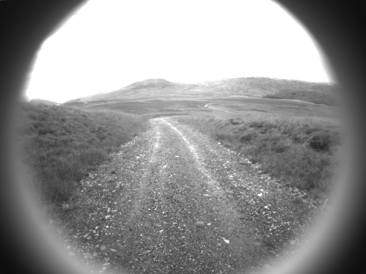
(a) LABEL:DB1

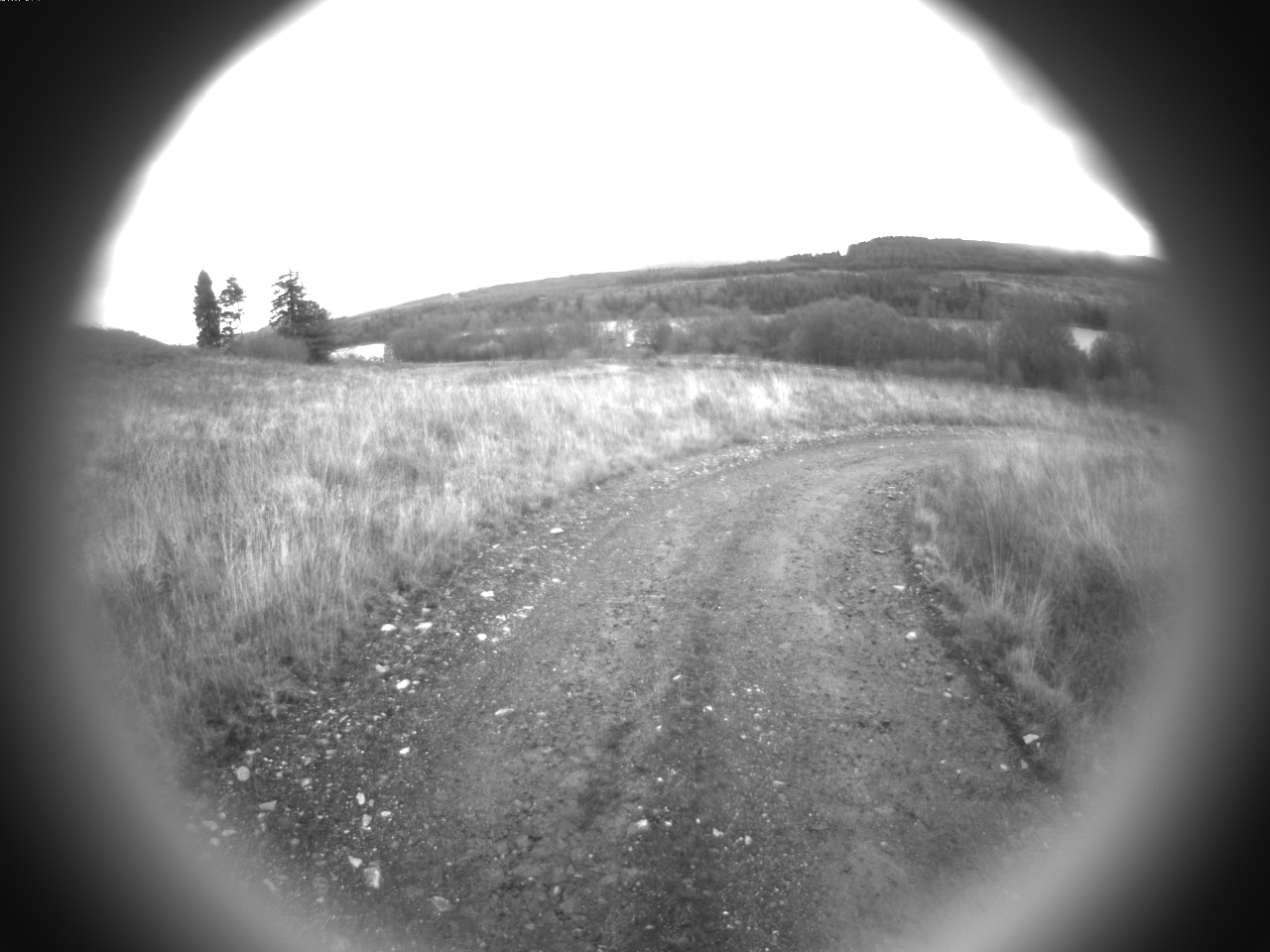
(b) LABEL:DB2

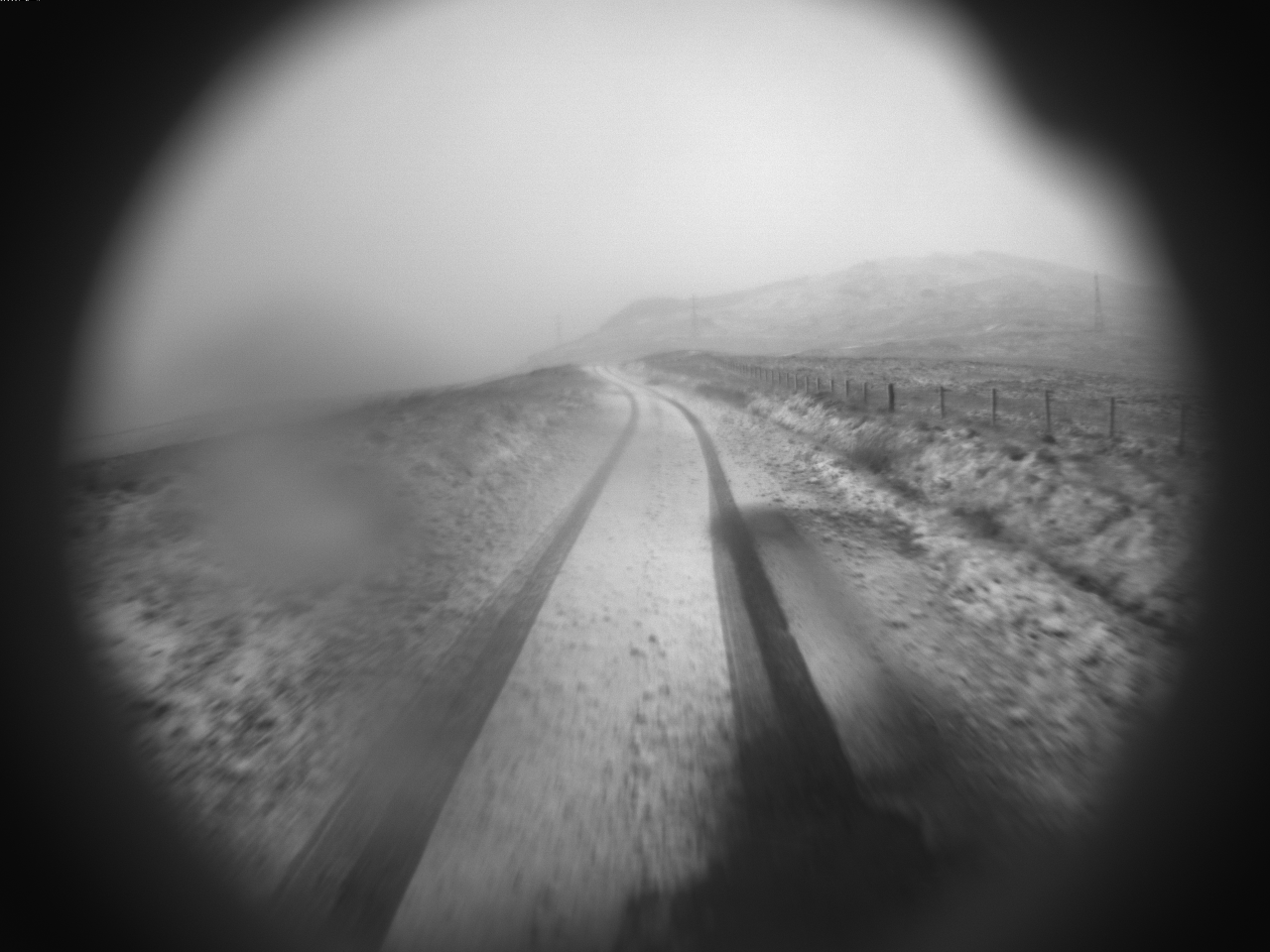
(c) LABEL:DB3

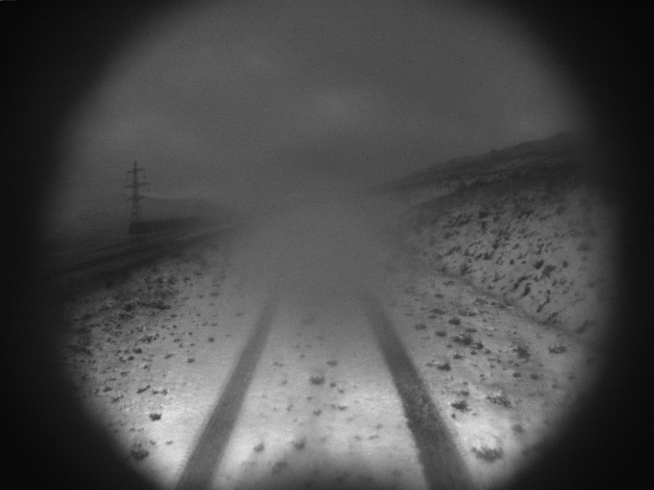
(d) LABEL:DB4

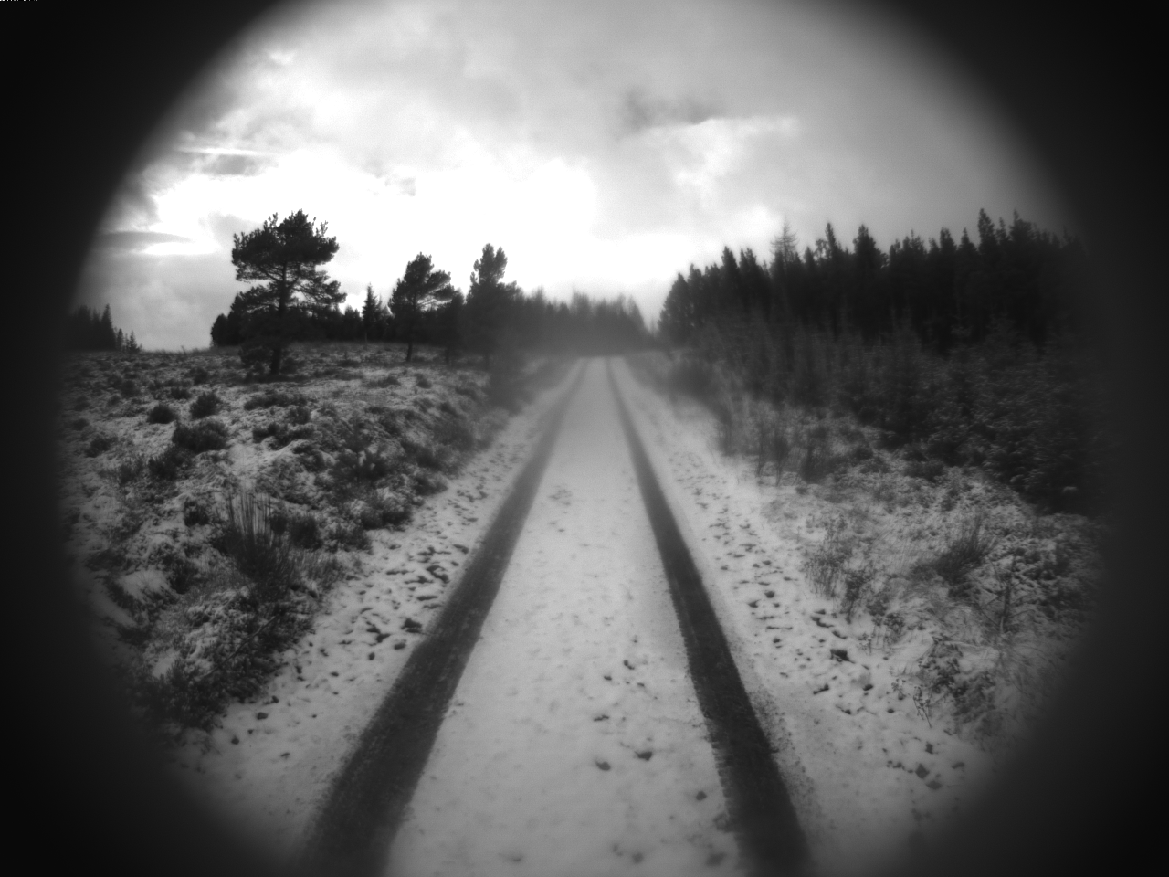
(e) LABEL:DH1

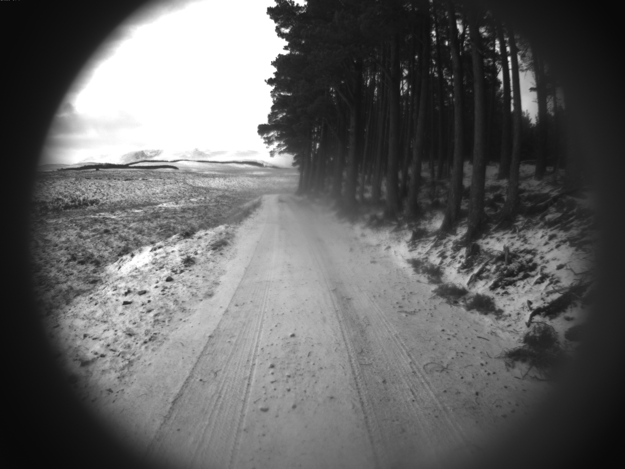
(f) LABEL:DH2

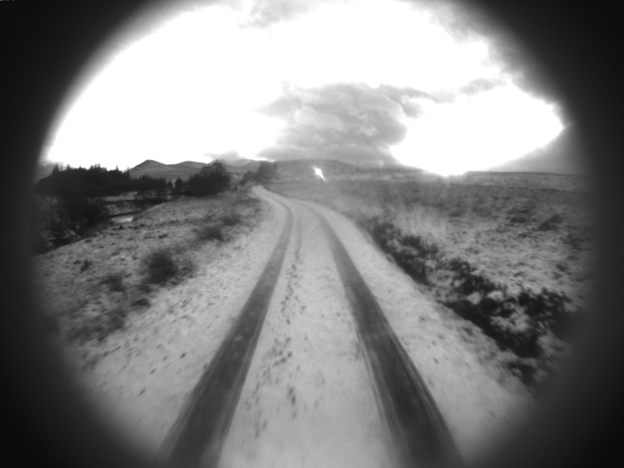
(g) LABEL:DH3

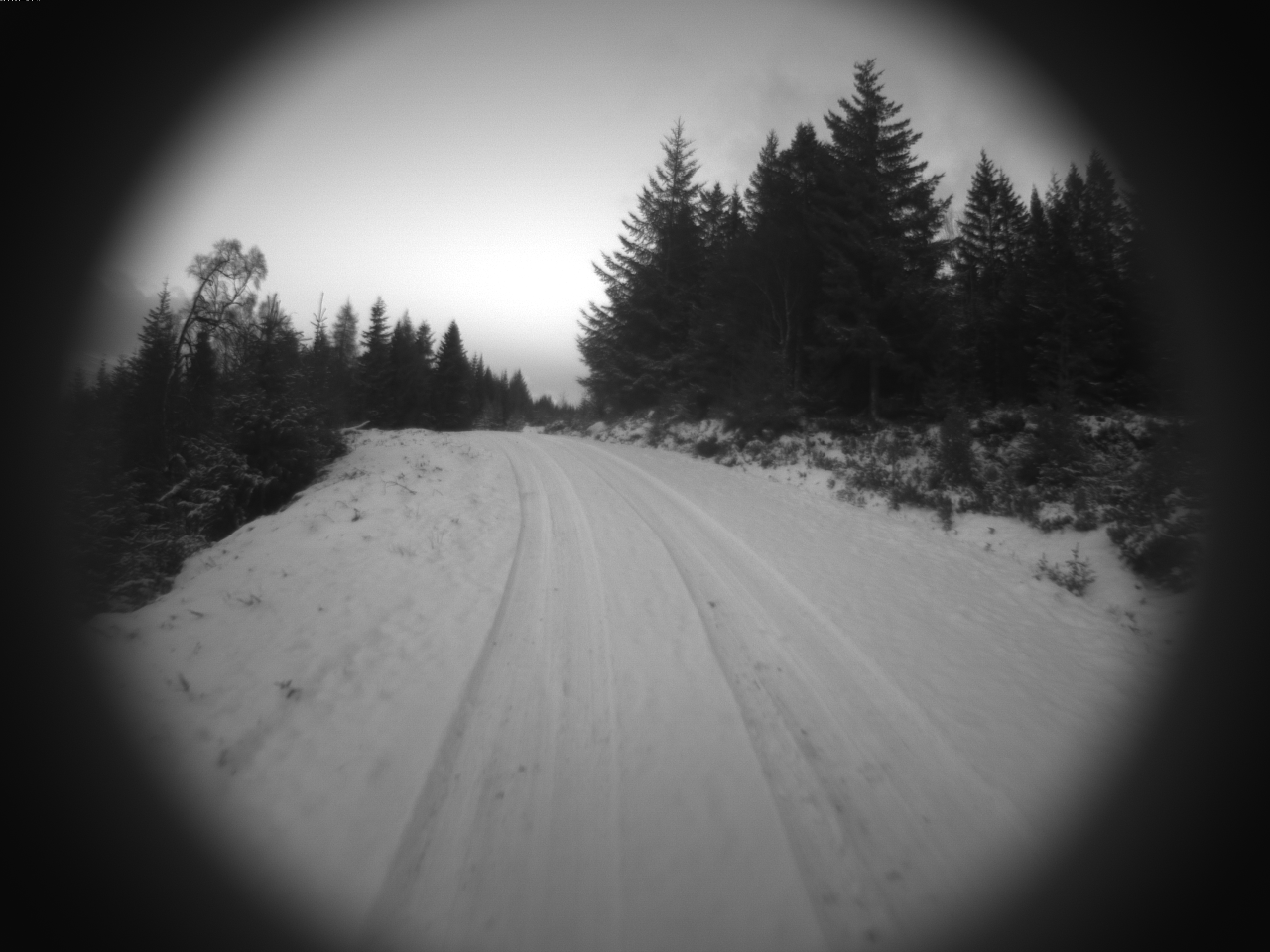
(h) LABEL:DM1

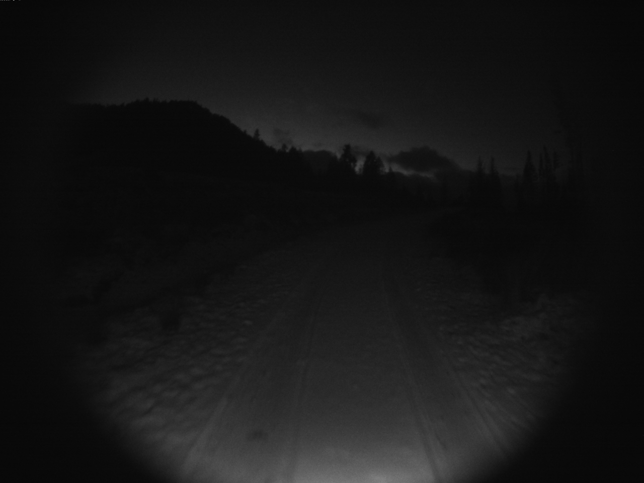
(i) LABEL:DM2

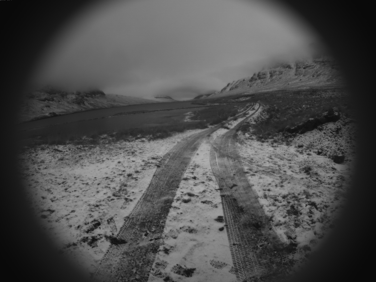
(j) LABEL:DA1

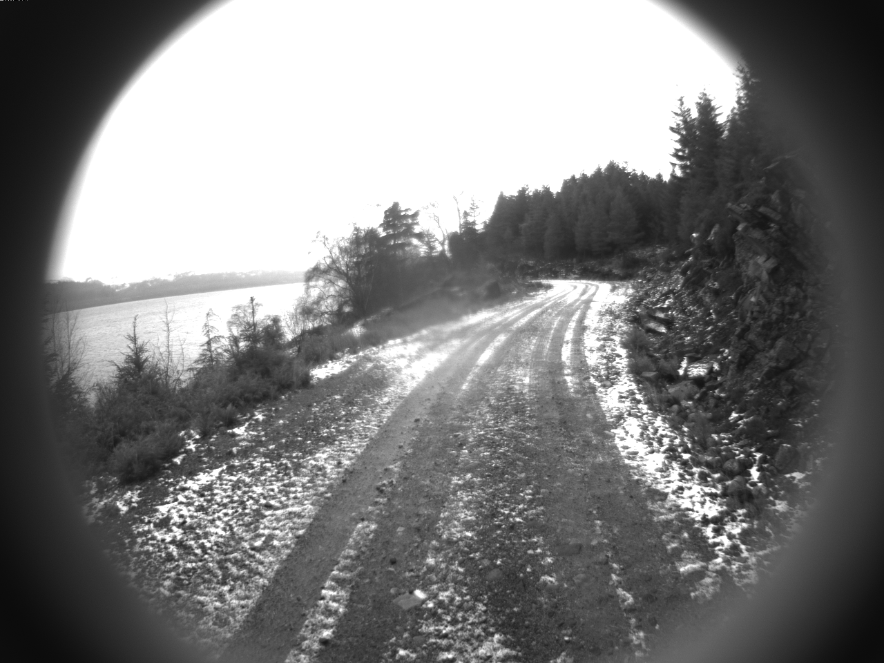
(k) LABEL:DA2

Figure 5: On-board camera images for each released foray in Sec. III-E. Note that as this dataset is radar-focused, we do not release these camera images, but they are included here to give a sense of the inclement collection conditions.

III-C Route 3: Maree

This is a $16.87\text{\,}\mathrm{km}$ route. The route is mountainous, in the elevated area to the south of Loch Laggan, see Fig. 8(a) (Top Middle). There are two ascents and descents as can be seen in Fig. 4 – with a descent halfway through the journey, and another at the end of the journey. The vehicle is primarily on a gravel track. Figs. 5(h) and 5(i) show images from the vehicle’s perspective from two outings along this route. Both of these feature heavy snow, with a completely covered track. In Fig. 5(i) the vehicle is driving in total darkness (with no artificial illumination beyond the vehicle’s spotlights as this is a very remote and isolated natural collection site). The outings are in the same direction, as per the ground truth matrix in Fig. 8(a) (Top Right), but within each outing itself we double back on parts of the route and return to the starting point along the same route we took to begin the route (c.f. the off diagonal matches in three parts of this matrix).

III-D Route 4: Two Lochs

This is a $20.62\text{\,}\mathrm{km}$ route across the entire estate. The route is alongside two lochs (Loch Laggan and Lochan na h-Earba), see Fig. 8(b) (Top Middle, where the lochs are on top of and the bottom of the image, respectively). Referring to the route in an anti-clockwise sense, while going alongside Loch Laggan the vehicle is on tarmac – it is otherwise on unpaved road for the rest of the route. Figs. 5(k) and 5(j) show images from the vehicle’s perspective of our two outings – these are completed after snow has fallen (in previous days), so melted somewhat, but while it is still very visible on the ground etc. The outings are in the opposite direction as shown by the off-diagonal matches in the ground truth matrix in Fig. 8(b) (Top Right). Note that the red elevation profile in Fig. 4 corresponds to the foray shown in Fig. 8(b) (Top Middle), and is very flat at approximately $400\text{\,}\mathrm{m}$ as the vehicle traverses alongside Lochan na h-Earba.

III-E Summary: Datasets provided

In summary, the datasets provided are listed below, including the date-string for the collection time and the site that they were collected at, with colours corresponding to Fig. 4.

• (Dataset 1)[DB1]: 2021-11-25-12-01-20 (Bellmouth)

• (Dataset 2)[DB2]: 2021-11-25-12-31-19 (Bellmouth)

• (Dataset 3)[DB3]: 2021-11-26-15-35-34 (Bellmouth)

• (Dataset 4)[DB4]: 2021-11-26-16-12-01 (Bellmouth)

• (Dataset 5)[DH1]: 2021-11-27-14-37-20 (Hydro)

• (Dataset 6)[DH2]: 2021-11-27-15-24-02 (Hydro)

• (Dataset 7)[DH3]: 2021-11-27-16-03-26 (Hydro)

• (Dataset 8)[DM1]: 2021-11-28-15-54-55 (Maree)

• (Dataset 9)[DM2]: 2021-11-28-16-43-37 (Maree)

• (Dataset 10)[DA1]: 2021-11-29-11-40-37 (Two Lochs)

• (Dataset 11)[DA2]: 2021-11-29-12-19-16 (Two Lochs)

These are shown in Fig. 5. We note that, beyond the weather and illumination effects discussed for each route above, some forays have lens adherents on the on-board camera (e.g. Figs. 5(c) and 5(d) in particular), motivating the use of radar in this sort of domain and for the localisation task.

IV Sensors & dataset format

At oxford-robotics-instiute.github.io/oord-dataset we provide for download time-stamped synchronised radar and GPS/INS.

IV-A Radar

This sensor is the same as that used for the Oxford Radar RobotCar Dataset [27], i.e. a Navtech CTS350-X Millimetre-Wave frequency-modulated continuous wave radar, $4\text{\,}\mathrm{Hz}$, $400\text{\,}$ measurements per rotation, $163\text{\,}\mathrm{m}$ range, $4.38\text{\,}\mathrm{cm}$ range resolution, $1.8\text{\,}\mathrm{\SIUnitSymbolDegree}$ beamwidth. The radar was mounted at the centre of the vehicle aligned to the vehicle axes.

Radar scans are stored as lossless-compressed PNG files in polar form with each row representing the sensor reading at each azimuth and each column representing the raw power return at a particular range.

IV-B GPS/INS

We use a Microstrain 3DM-RQ1-45 GPS/INS. This sensor has direct satellite and inertial measurements, and computes position, velocity, and attitude. To provide accurate readings, it uses a triaxial accelerometer, gyroscope, magnetometer, and temperature sensors, as well as a pressure altimeter. Furthermore, dual on-board processors run a Extended Kalman Filter (EKF).

V Software & experimental tools

At github.com/mttgdd/oord-dataset and huggingface.co/mttgdd/oord-models we provide a software tools to support the use of this dataset.

V-A Downloads & data loaders

Similarly to [27], we provide data loaders to work with the radar data format, which as per Sec. IV-A are released in raw polar format, but can be easily transformed into Cartesian format with our SDK.

For working with driven sequences, we provide a basic iterable Dataset class which returns each radar scan paired with its closest (in a timestamp sense) GPS/INS reading (Sec. IV-B).

We also provide a batch download script to rapidly access the data.

V-B Radar place recognition evaluation

We evaluate place recognition performance by comparing “distance matrices” in the ground truth space given by GPS, as shown by example in Figs. 3 and 8 (Top Right) to distance matrices composed of e.g. pairwise distances between vectors representing radar scans (see Sec. VI) or some other similarity measurement. These matrices have heights given by the number of radar scans in a “query” foray and widths similarly for a “reference” foray. Highlighted regions are such that those radar scan pairs have locations given by GPS which are within $25\text{\,}\mathrm{m}$ (this threshold being configurable in our SDK). In these, interesting features to note are the off-diagonal revisits, which represent traversals in the opposite direction. This is especially important in the radar modality as the sensor has a $360\text{\,}\mathrm{\SIUnitSymbolDegree}$ field-of-view.

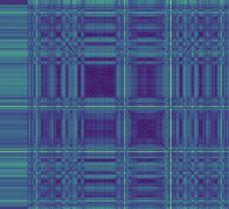
(a) RingKey, LABEL:B1

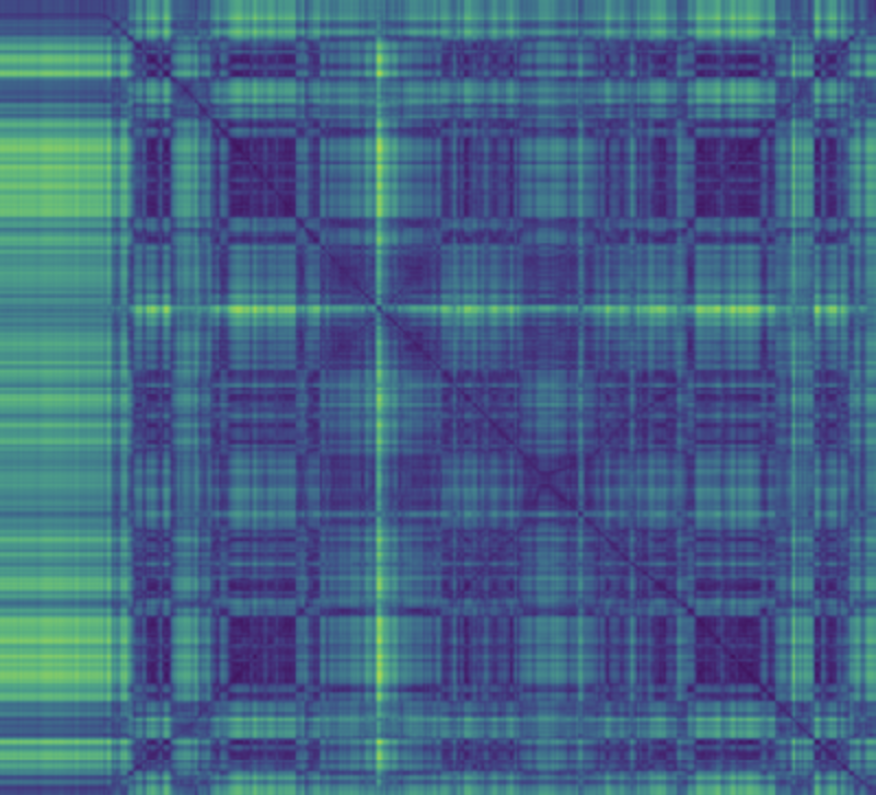
(b) AlexNet, LABEL:B8

(c) RaPlace, LABEL:B2

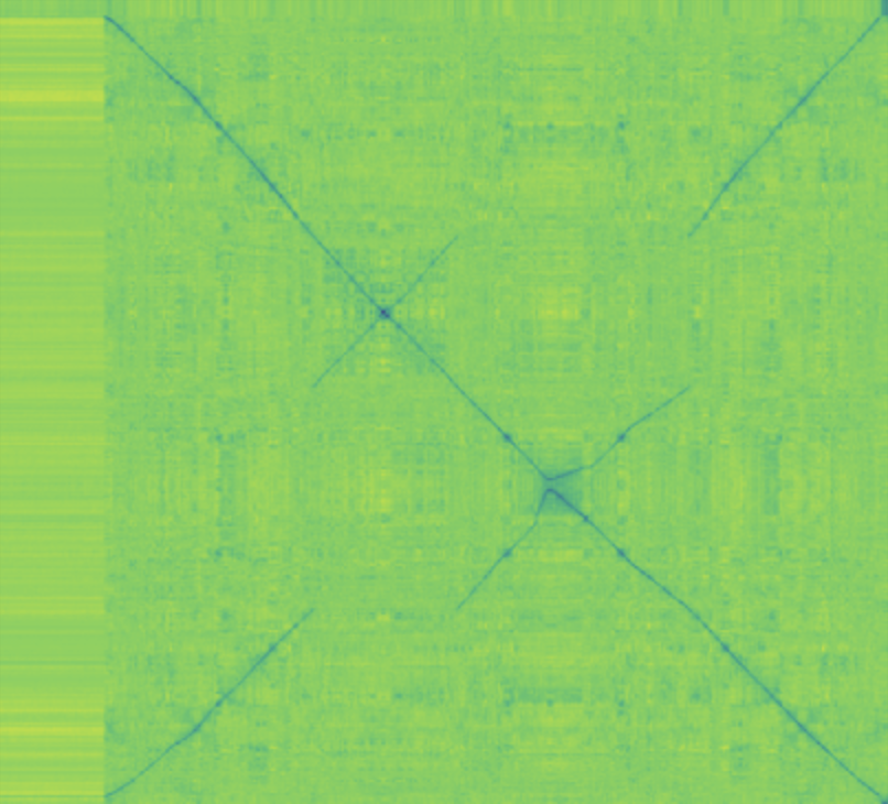
(d) RadVLAD, LABEL:B3

Figure 6: Example embedding distance matrices between a live trajectory (rows) and a reference trajectory (columns) in this case 2021-11-25-12-31-19 and 2021-11-25-12-01-20 from bellmouth, respectively. LABEL:B2 and LABEL:B3 are the most distinctive, being radar-specific methods.

Then, Recall@N refers to the percentage of query scans which result in at least one successful localisation (i.e. resulting in a returned location within $25\text{\,}\mathrm{m}$ of the query location) when accepting as candidates all of the $N$ nearest neighbours in the embedding space. This is a commonly used metric and threshold, as in visual place recognition [36, 37]. Note that in Figs. 3 and 8 the true positives are “thickened” for visualisation purposes, to $100\text{\,}\mathrm{m}$, but we experiment in Sec. VII with $25\text{\,}\mathrm{m}$.

For this we use a “difference matrix” in Fig. 6 with the embedding distances (Euclidean) between live and map features. Localisation is successful if the nearest neighbour for a query embedding (rows) is a reference embedding (column) which is in truth (c.f. the ground truth matrices in Fig. 3(a) Top Right) is close to the query location in physical space.

V-C Radar place recognition with neural networks

As will be discussed below, we evaluate a family of learned methods on our dataset. This includes a pretrained and frozen backbone feature extractor along with a pooling layer which is fine-tuned on radar data from this dataset, and we release these weights at huggingface.co/mttgdd/oord-models , with this being, to our knowledge, the first open-sourced learned radar place recognition system.

V-D Open-source radar place recognition methods

As below in Sec. VI, our SDK includes either (1) new implementations of or (2) imports, as submodules, of other open-source radar place recognition systems [14, 22, 35]. Experiments on novel systems can be quickly run over all pairs of trajectories discussed in Sec. III-E, and prepared in the format of Tab. III, by a common .yaml configuration format.

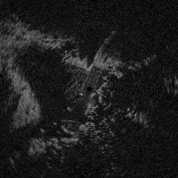
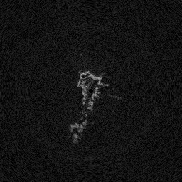
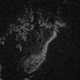
(a) The maree dataset shares outgoing and incomings routes in opposite directions, with a single-direction loop midway.

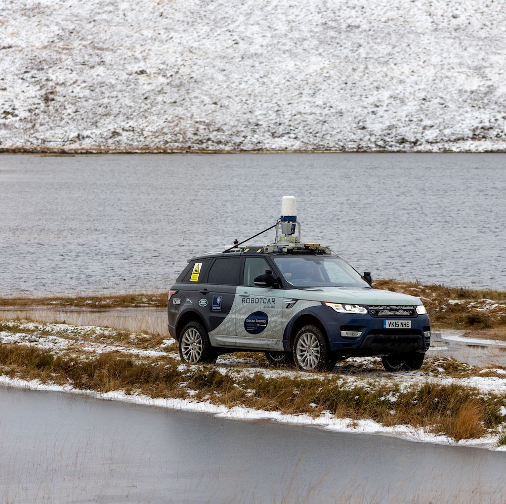
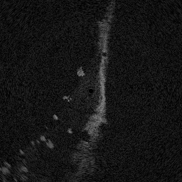
(b) The twolochs dataset is the most extensive we provide, and is collected over a journey featuring (1) a tarmac road under tree cover alongside a Loch Laggan (top), (2) a gravel track over the shoulder of a mountain, (3) a partially submerged track fording a loch, (4) a gravel track alongside Lochan na h-Earba, and (5) a gravel track descending a mountainside to the start location.

Figure 8: The hydro and maree datasets, with GPS traces, ground truth matrices, and sample scans.

VI Examples

We demonstrate the utility of our dataset as a novel radar place recognition benchmark using the evaluation method described in Sec. V-B. We also show that the GPS/INS described in Sec. IV-B can be put to good use in supervising learned radar place recognition methods.

Therefore, we demonstrate implementations of the following methods with our dataset:

• (Baseline 1)[B1]: RingKey as a component of ScanContext [38] averages point cloud contents at a fixed distance around the vehicle (thus being rotation invariant). Note, for this we do not use the orientation refinement of ScanContext, as distances between row-reduced vectors and orientation scores are separate, i.e. these form a hierarchy of localisers. To be clear, this is different to LABEL:B2 below, where the maximum circular cross-correlation is the score used for similarity between scans (with no initial score used to reduce the candidate set).

• (Baseline 2)[B2]: RaPlace [22] measures the similarity score between radar scans by using Radon-transformed sinogram images and cross-correlation in the frequency domain. This gives rigid transform invariance during place recognition, and supresses the effects of radar multipath and ring noises.

• (Baseline 3)[B3]: Open-RadVLAD [35] uses only the polar representation. Also, for partial translation invariance and robustness to signal noise, it uses only a 1D Fourier Transform along radial returns. It also achieves rotational invariance and a very discriminative descriptor space by building a vector of locally aggregated descriptors (VLAD).

• (Baseline 4)[B4]: Here we train radar-specific neural network models – using ResNet18 [39] as a backbone feature extractor and NetVLAD [36] as a pooling layer (with $64$ clusters). Inputs are polar radar scans of $128\times 128$ resolution and embeddings are $128$-dimensional. The radar returns are replicated $3$ times at the input in order to form a $3$-channel image. We start with pretrained weights learned against ImageNet [40] and then, in an unsupervised learning step, initialise the NetVLAD cluster centres by k-means++ [41] over the deep features extracted from the reference trajectory radar frames.

• (Baseline 5)[B5], (Baseline 6)[B6], (Baseline 7)[B7], (Baseline 8)[B8], (Baseline 9)[B9]: Here we show that the plug-and-play ability of our dataset with respect to widely available pretrained networks, to accelerate research in this area. We use specifically the pytorch/vision:v0.10.0 models available at pytorch.org/hub as well as the gmberton/cosplace models available at github.com/gmberton/CosPlace . This covers MobileNet [42] LABEL:B6, GoogleNet [43] LABEL:B7, AlexNet [44] LABEL:B8, and VGG19 [45] LABEL:B9, which are all trained for ImageNet classification and thus not specialised for place recognition but represent inputs in terms of wide variety of concepts and features. It also covers CosPlace (ResNet18-512) [37] LABEL:B5 which is specifically trained for place recognition – but not specifically for the radar modality, in contrast to LABEL:B4.

Sec. VII presents a comprehensive comparison of these example baselines over all pairs of trajectories from our dataset.

	LABEL:DB2-vs-LABEL:DB1	LABEL:DH1-vs-LABEL:DH2	LABEL:DH1-vs-LABEL:DH3	LABEL:DM1-vs-LABEL:DM2	LABEL:DA2-vs-LABEL:DA1
LABEL:B1	94.29 / 97.53 / 98.24	91.15 / 93.57 / 93.78	94.06 / 95.80 / 96.00	91.76 / 97.22 / 98.42	72.96 / 82.28 / 84.71
LABEL:B2	98.45 / 98.73 / 98.94	92.65 / 93.89 / 93.94	95.34 / 95.85 / 95.85	94.28 / 99.15 / 99.40	85.82 / 87.69 / 88.25
LABEL:B3	98.87 / 99.79 / 99.93	93.51 / 94.10 / 94.16	96.00 / 96.16 / 96.16	96.88 / 99.06 / 99.32	84.27 / 87.36 / 88.25
LABEL:B4	97.67 / 98.52 / 98.87	93.78 / 94.26 / 94.37	95.70 / 99.59 / 99.95	97.14 / 99.06 / 99.44	5.41 / 10.98 / 16.23
LABEL:B5	90.49 / 97.25 / 98.10	92.76 / 93.83 / 93.83	94.72 / 95.85 / 95.85	89.11 / 97.91 / 98.72	4.53 / 10.10 / 15.51
LABEL:B6	90.70 / 97.04 / 98.45	91.96 / 93.62 / 93.83	93.14 / 95.49 / 95.75	87.92 / 96.67 / 98.25	17.55 / 40.07 / 50.44
LABEL:B7	94.50 / 98.38 / 98.80	92.28 / 93.83 / 93.83	93.70 / 95.54 / 95.80	90.61 / 97.27 / 98.42	23.18 / 47.19 / 58.22
LABEL:B8	74.91 / 92.39 / 95.28	82.79 / 91.31 / 92.60	83.91 / 92.78 / 94.62	65.16 / 86.93 / 92.10	14.74 / 35.87 / 47.08
LABEL:B9	72.73 / 90.49 / 94.71	81.29 / 90.40 / 91.96	84.07 / 93.14 / 94.31	69.43 / 87.15 / 91.97	9.71 / 21.80 / 31.29

TABLE III: Recall@1/5/10 localisation success rate (%) for all example methods defined in Sec. VI and discussed in Sec. VII over $5$ pairs of trajectories from our dataset.

VII Results

As can be seen in Tab. III, considering that all of each of the routes is at minimum $9\text{\,}\mathrm{km}$ in length (seeTab. II), all radar-specific methods perform very well, with in excess of $90\text{\,}\mathrm{\char 37\relax}$ for even Recall@1 i.e. when relying on only a single nearest neighbour in embedding space look up.

Overall the best performing methods are LABEL:B3 Open-RadVLAD [35], LABEL:B4 ResNet18-NetVLAD, and LABEL:B2 RaPlace [22].

There is in fact a precipitous drop in localisation success rate for all methods in LABEL:DA1-vs-LABEL:DA2 in twolochs. We attribute this to twolochs (Sec. III-D) being the longest route (there therefore being more candidate scans to match to – i.e. the search space being larger). In Fig. 8(b) this can be seen in the ground truth matrix (Top Right) by the large region to the right of the white strip, where the query trajectory ends at Loch Laggan and therefore only overlaps with the reference trajectory (Middle Right in Fig. 8(b)) for approximately $40\text{\,}\mathrm{\char 37\relax}$ of the route, with the reference trajectory continuing north-east all the way along both bodies of water in Loch Laggan. This may also be due to the long periods driven along either Loch Laggan or Lochan na h-Earba where there is a dearth of distinctive scenery in an entire hemisphere of the radar scan. An example scan from this type of scene can be seen in the third Cartesian frame in Fig. 8(b) (Bottom). Therefore, twolochs is a useful test setting for robust recognition with vast maps as well as with featureless scenery, as radar place recognition matures. For this challenging route, only radar-specific methods perform well and we have LABEL:B2 RaPlace performing best, with LABEL:B3 Open-RadVLAD matching it in Recall@10. LABEL:B4 ResNet18-NetVLAD performs poorly on this pair of trajectories, likely due to clustering of the reference trajectory features, many of which are irrelevant to the query trajectory.

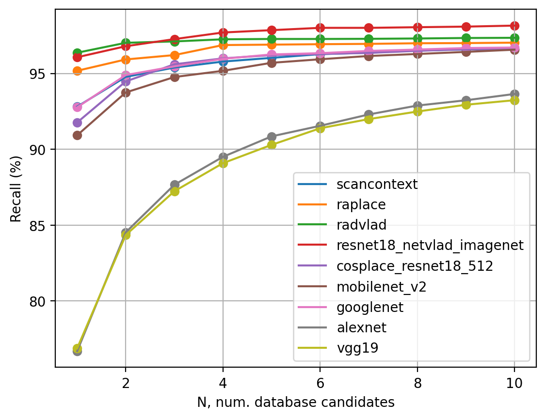
Figure 9: Recall@N localisation success rate, as described in Sec. V-B. LABEL:B2 (RaPlace), LABEL:B3 (RadVLAD), and LABEL:B4 (ResNet18-NetVLAD) perform best. The approach customised to radar data, LABEL:B4, outstrips others when more database candidates are retrieved.

Fig. 9 shows the Recall@N curves corresponding to Tab. III, averaged over all pairs of trajectories. From this we can see that LABEL:B3 Open-RadVLAD and LABEL:B4 ResNet18-NetVLAD perform best with LABEL:B3 Open-RadVLAD slightly better at lower recalled candidates (and thus perhaps being better suited to efficient deployment) but LABEL:B4 ResNet18-NetVLAD performing slightly better when more candidates are recalled. LABEL:B2 RaPlace is worse than either of these at fewer recalled candidates but approaches LABEL:B3 Open-RadVLAD when more database candidates are retrieved.

VIII Conclusion

We have presented a novel radar dataset, carefully gathered under unique and challenging conditions. This dataset has been crafted to catalyse advancements in the emerging field of radar place recognition. We explored the use of our dataset in this task over a series of comprehensive experiments and evaluations, carried out across various open-source radar place recognition systems. This was not only to showcase the dataset but also to establish a robust platform for future research in this evolving area.

In the future, we would like to document new radar place recognition performance against this benchmark, and plan to do this online at e.g. paperswithcode.com/datasets .

References

- [1] K. Harlow, H. Jang, T. D. Barfoot, A. Kim, and C. Heckman, “A new wave in robotics: Survey on recent mmwave radar applications in robotics,” arXiv preprint arXiv:2305.01135, 2023.
- [2] A. Venon, Y. Dupuis, P. Vasseur, and P. Merriaux, “Millimeter wave fmcw radars for perception, recognition and localization in automotive applications: A survey,” IEEE Transactions on Intelligent Vehicles, vol. 7, no. 3, pp. 533–555, 2022.
- [3] S. H. Cen and P. Newman, “Precise ego-motion estimation with millimeter-wave radar under diverse and challenging conditions,” in IEEE International Conference on Robotics and Automation (ICRA), 2018, pp. 6045–6052.
- [4] D. Barnes, R. Weston, and I. Posner, “Masking by moving: Learning distraction-free radar odometry from pose information,” arXiv preprint arXiv:1909.03752, 2019.
- [5] Y. S. Park, Y.-S. Shin, and A. Kim, “Pharao: Direct radar odometry using phase correlation,” in 2020 IEEE International Conference on Robotics and Automation (ICRA). IEEE, 2020, pp. 2617–2623.
- [6] P.-C. Kung, C.-C. Wang, and W.-C. Lin, “A normal distribution transform-based radar odometry designed for scanning and automotive radars,” in 2021 IEEE International Conference on Robotics and Automation (ICRA). IEEE, 2021, pp. 14 417–14 423.
- [7] K. Burnett, A. P. Schoellig, and T. D. Barfoot, “Do we need to compensate for motion distortion and doppler effects in spinning radar navigation?” IEEE Robotics and Automation Letters, vol. 6, no. 2, pp. 771–778, 2021.
- [8] D. Adolfsson, M. Magnusson, A. Alhashimi, A. J. Lilienthal, and H. Andreasson, “Cfear radarodometry-conservative filtering for efficient and accurate radar odometry,” in 2021 IEEE/RSJ International Conference on Intelligent Robots and Systems (IROS). IEEE, 2021, pp. 5462–5469.
- [9] K. Burnett, D. J. Yoon, A. P. Schoellig, and T. D. Barfoot, “Radar odometry combining probabilistic estimation and unsupervised feature learning,” arXiv preprint arXiv:2105.14152, 2021.
- [10] R. Aldera, M. Gadd, D. De Martini, and P. Newman, “What goes around: Leveraging a constant-curvature motion constraint in radar odometry,” IEEE Robotics and Automation Letters, vol. 7, no. 3, pp. 7865–7872, 2022.
- [11] D. Barnes and I. Posner, “Under the radar: Learning to predict robust keypoints for odometry estimation and metric localisation in radar,” in International Conference on Robotics and Automation (ICRA), 2020.
- [12] H. Yin, Y. Wang, L. Tang, and R. Xiong, “Radar-on-lidar: metric radar localization on prior lidar maps,” in 2020 IEEE International Conference on Real-time Computing and Robotics (RCAR). IEEE, 2020, pp. 1–7.
- [13] H. Yin, R. Chen, Y. Wang, and R. Xiong, “Rall: end-to-end radar localization on lidar map using differentiable measurement model,” IEEE Transactions on Intelligent Transportation Systems, 2021.
- [14] G. Kim, Y. S. Park, Y. Cho, J. Jeong, and A. Kim, “Mulran: Multimodal range dataset for urban place recognition,” in International Conference on Robotics and Automation (ICRA), 2020.
- [15] Ş. Săftescu, M. Gadd, D. De Martini, D. Barnes, and P. Newman, “Kidnapped radar: Topological radar localisation using rotationally-invariant metric learning,” in 2020 IEEE International Conference on Robotics and Automation (ICRA). IEEE, 2020, pp. 4358–4364.
- [16] W. Wang, P. P. de Gusmo, B. Yang, A. Markham, and N. Trigoni, “RadarLoc: Learning to Relocalize in FMCW Radar,” in IEEE International Conference on Robotics and Automation (ICRA), 2021.
- [17] H. Yin, X. Xu, Y. Wang, and R. Xiong, “Radar-to-lidar: Heterogeneous place recognition via joint learning,” Frontiers in Robotics and AI, 2021.
- [18] J. Komorowski, M. Wysoczanska, and T. Trzcinski, “Large-scale topological radar localization using learned descriptors,” in Neural Information Processing: 28th International Conference, ICONIP 2021, Sanur, Bali, Indonesia, December 8–12, 2021, Proceedings, Part II 28. Springer, 2021, pp. 451–462.
- [19] M. Gadd, D. De Martini, and P. Newman, “Contrastive learning for unsupervised radar place recognition,” in 2021 20th International Conference on Advanced Robotics (ICAR). IEEE, 2021, pp. 344–349.
- [20] S. Lu, X. Xu, H. Yin, Z. Chen, R. Xiong, and Y. Wang, “One ring to rule them all: Radon sinogram for place recognition, orientation and translation estimation,” in 2022 IEEE/RSJ International Conference on Intelligent Robots and Systems (IROS). IEEE, 2022, pp. 2778–2785.
- [21] K. Cait, B. Wang, and C. X. Lu, “Autoplace: Robust place recognition with single-chip automotive radar,” in 2022 International Conference on Robotics and Automation (ICRA). IEEE, 2022, pp. 2222–2228.
- [22] H. Jang, M. Jung, and A. Kim, “Raplace: Place recognition for imaging radar using radon transform and mutable threshold,” arXiv preprint arXiv:2307.04321, 2023.
- [23] J. Yuan, P. Newman, and M. Gadd, “Off the Radar: Variational Uncertainty-Aware Unsupervised Radar Place Recognition for Introspective Querying and Map Maintenance,” in IEEE/RSJ International Conference on Intelligent Robots and Systems (IROS), 2023.
- [24] Z. Hong, Y. Petillot, and S. Wang, “Radarslam: Radar based large-scale slam in all weathers,” in IEEE/RSJ International Conference on Intelligent Robots and Systems (IROS), 2020.
- [25] D. Wang, Y. Duan, X. Fan, C. Meng, J. Ji, and Y. Zhang, “Maroam: Map-based radar slam through two-step feature selection,” arXiv preprint arXiv:2210.13797, 2022.
- [26] T. Peynot, S. Scheding, and S. Terho, “The marulan data sets: Multi-sensor perception in a natural environment with challenging conditions,” The International Journal of Robotics Research, vol. 29, no. 13, pp. 1602–1607, 2010.
- [27] D. Barnes, M. Gadd, P. Murcutt, P. Newman, and I. Posner, “The oxford radar robotcar dataset: A radar extension to the oxford robotcar dataset,” in International Conference on Robotics and Automation (ICRA), 2020.
- [28] M. Sheeny, E. De Pellegrin, S. Mukherjee, A. Ahrabian, S. Wang, and A. Wallace, “Radiate: A radar dataset for automotive perception in bad weather,” in 2021 IEEE International Conference on Robotics and Automation (ICRA). IEEE, 2021, pp. 1–7.
- [29] K. Burnett, D. J. Yoon, Y. Wu, A. Z. Li, H. Zhang, S. Lu, J. Qian, W.-K. Tseng, A. Lambert, K. Y. Leung et al., “Boreas: A multi-season autonomous driving dataset,” The International Journal of Robotics Research, vol. 42, no. 1-2, pp. 33–42, 2023.
- [30] R. Tagiew, M. Köppel, K. Schwalbe, P. Denzler, P. Neumaier, T. Klockau, M. Boekhoff, P. Klasek, and R. Tilly, “Osdar23: Open sensor data for rail 2023,” arXiv preprint arXiv:2305.03001, 2023.
- [31] M. Gadd, D. De Martini, and P. Newman, “Look around you: Sequence-based radar place recognition with learned rotational invariance,” in 2020 IEEE/ION Position, Location and Navigation Symposium (PLANS). IEEE, 2020, pp. 270–276.
- [32] Z. Hong, Y. Petillot, A. Wallace, and S. Wang, “Radarslam: A robust simultaneous localization and mapping system for all weather conditions,” The International Journal of Robotics Research, 2022.
- [33] D. Adolfsson, M. Karlsson, V. Kubelka, M. Magnusson, and H. Andreasson, “Tbv radar slam: trust but verify loop candidates,” arXiv preprint arXiv:2301.04397, 2023.
- [34] H. Jang, M. Jung, and A. Kim, “RaPlace: Place Recognition for Imaging Radar using Radon Transform and Mutable Threshold,” in IEEE/RSJ International Conference on Intelligent Robots and Systems (IROS), 2023.
- [35] M. Gadd and P. Newman, “Open-RadVLAD: Fast and Robust Radar Place Recognition,” arXiv preprint arXiv:2401.15380, 2024.
- [36] R. Arandjelovic, P. Gronat, A. Torii, T. Pajdla, and J. Sivic, “Netvlad: Cnn architecture for weakly supervised place recognition,” in IEEE Conference on Computer Vision and Pattern Recognition, 2016.
- [37] G. Berton, C. Masone, and B. Caputo, “Rethinking visual geo-localization for large-scale applications,” in IEEE/CVF Conference on Computer Vision and Pattern Recognition, 2022, pp. 4878–4888.
- [38] G. Kim and A. Kim, “Scan context: Egocentric spatial descriptor for place recognition within 3d point cloud map,” in IEEE/RSJ International Conference on Intelligent Robots and Systems (IROS), 2018.
- [39] K. He, X. Zhang, S. Ren, and J. Sun, “Deep residual learning for image recognition,” in Proceedings of the IEEE conference on computer vision and pattern recognition, 2016, pp. 770–778.
- [40] J. Deng, W. Dong, R. Socher, L.-J. Li, K. Li, and L. Fei-Fei, “Imagenet: A large-scale hierarchical image database,” in 2009 IEEE conference on computer vision and pattern recognition. Ieee, 2009, pp. 248–255.
- [41] D. Arthur and S. Vassilvitskii, “K-means++ the advantages of careful seeding,” in eighteenth annual ACM-SIAM symposium on Discrete algorithms, 2007, pp. 1027–1035.
- [42] M. Sandler, A. Howard, M. Zhu, A. Zhmoginov, and L.-C. Chen, “Mobilenetv2: Inverted residuals and linear bottlenecks,” in IEEE conference on computer vision and pattern recognition, 2018.
- [43] C. Szegedy, W. Liu, Y. Jia, P. Sermanet, S. Reed, D. Anguelov, D. Erhan, V. Vanhoucke, and A. Rabinovich, “Going deeper with convolutions,” in IEEE conference on computer vision and pattern recognition, 2015.
- [44] A. Krizhevsky, I. Sutskever, and G. E. Hinton, “Imagenet classification with deep convolutional neural networks,” Advances in neural information processing systems, vol. 25, 2012.
- [45] K. Simonyan and A. Zisserman, “Very deep convolutional networks for large-scale image recognition,” arXiv preprint arXiv:1409.1556, 2014.