Model	$\psi(\boldsymbol{y};\boldsymbol{\Lambda})$	Boundary growth condition on $\boldsymbol{\Lambda}$
GBM	$(2\pi)^{-\frac{d}{2}}(\operatorname{det}(\boldsymbol{\tilde{\Sigma}}))^{-\frac{1}{2}}\exp\left(-\frac{1}{2}(\boldsymbol{y}^{\prime}\boldsymbol{\tilde{\Sigma}}^{-1}\boldsymbol{y})\right)$	$T\boldsymbol{\Sigma}-\boldsymbol{\tilde{\Sigma}}^{-1}\succeq 0$
VG	$\frac{\Gamma\left(\frac{\tilde{\nu}+d}{2}\right)}{\Gamma\left(\frac{\tilde{\nu}}{2}\right)\tilde{\nu}^{\frac{d}{2}}\pi^{\frac{d}{2}}\sqrt{\operatorname{det}(\boldsymbol{\tilde{\Sigma}})}}\left(1+\frac{1}{\tilde{\nu}}\left(\boldsymbol{y}^{\prime}\boldsymbol{\tilde{\Sigma}}\boldsymbol{y}\right)\right)^{-\frac{\tilde{\nu}+d}{2}}$	$\tilde{\nu}=\frac{2T}{\nu}-d$,   and   $\boldsymbol{\Sigma}-\boldsymbol{\tilde{\Sigma}}^{-1}\succeq 0$   or $\tilde{\nu}\leq\frac{2T}{\nu}-d$,   and   $\boldsymbol{\tilde{\Sigma}}=\boldsymbol{\Sigma}^{-1}$.
NIG	$(2\pi)^{-\frac{d}{2}}(\operatorname{det}(\boldsymbol{\tilde{\Sigma}}))^{-\frac{1}{2}}\left(\frac{\boldsymbol{y}^{\prime}\boldsymbol{\tilde{\Sigma}}^{-1}\boldsymbol{y}}{2}\right)^{\frac{v}{2}}K_{v}\left(\sqrt{2\boldsymbol{y}^{\prime}\boldsymbol{\tilde{\Sigma}}^{-1}\boldsymbol{y}}\right)$	$\delta^{2}T^{2}\boldsymbol{\Delta}-2\boldsymbol{\tilde{\Sigma}}^{-1}\succeq 0$

3.2.1 Domain transformation for the GBM model

Case of independent assets:

To simplify the preliminary analysis, we considered the case in which the stock price processes are independent. Consequently, the characteristic function of the pricing model can be written as the product of univariate characteristic functions; hence, ϕ^GBM_X_T(z) = ∏_j = 1^d ϕ^GBM_X^j_T(z_j), z∈C^d, ℑ[z] ∈δ^GBM_X where ϕ^GBM_X^j_T(z_j) := exp(rT - i σj2T2z_j - σj2T2z_j^2), z_j ∈C, ℑ[z_j] ∈δ^GBM_X Because $\phi^{GBM}_{X^{j}_{T}}(z_{j})$ is a Gaussian function, it is natural to propose that the domain transformation density is also Gaussian, in the form of $\psi^{nor}(\boldsymbol{y})=\prod_{j=1}^{d}\psi^{nor}_{j}(y_{j})$, where ψ^nor_j(y_j) := exp(- yj22~σ2j)2 ~σj2,  y_j ∈R,   ~σ_j ¿ 0, and applying the change of variable (LABEL:eq:change_of_variable), the transformed integrand is

(3.5) $$\small\tilde{g}(\boldsymbol{u}):=(2\pi)^{-d}e^{-rT}e^{-\boldsymbol{R}^{\prime}\boldsymbol{X}_{0}}\Re\left[e^{\mathrm{i}(\Psi_{nor}^{-1}(\boldsymbol{u}))^{\prime}\boldsymbol{X}_{0}}\widehat{P}(\Psi_{nor}^{-1}(\boldsymbol{u})+\mathrm{i}\boldsymbol{R})\prod_{j=1}^{d}\frac{\phi^{GBM}_{X^{j}_{T}}(\Psi_{nor}^{-1}(u_{j})+\mathrm{i}R_{j})}{\psi^{nor}_{j}(\Psi_{nor}^{-1}(u_{j}))}\right]\boldsymbol{u}\in[0,1],\boldsymbol{R}\in\delta^{GBM}_{V}.$$

After specifying the functional form of $\psi^{nor}_{j}(y_{j})$, the aim is to determine an appropriate choice of the parameters $\{\tilde{\sigma}_{j}\}_{j=1}^{d}$. The function $r^{GBM}_{j}(\cdot)$ is defined as the ratio of the characteristic function of the variable $X^{j}_{T}$ and the artificially introduced density $\psi^{nor}_{j}(\cdot)$: r^GBM_j(u_j) := ϕGBMXjT(Ψnor-1(uj)+ i Rj)ψnorj(Ψnor-1(uj)), u_j ∈[0,1], R ∈δ^GBM_V. The parameters $\{\tilde{\sigma}_{j}\}_{j=1}^{d}$ should be set to control the growth of the function $r^{GBM}_{j}(\cdot)$ near the boundary of $[0,1]$ as follows: lim_u_j →0 ∣r^GBM_j(u_j) ∣¡ ∞,   ∀  j ∈I_d ⇔lim_u_j →0 ∣~g(u) ∣¡ ∞,   ∀  j ∈I_d. By symmetry of the integrand $g(\cdot)$ and the proposal density $\psi^{nor}(\cdot)$ around the origin, it is sufficient to control the behavior of the transformed integrand as $u_{j}\to 0$ to ensure that it is also controlled at all $2^{d}$ corners of $[0,1]^{d}$. Moreover, we set $\boldsymbol{R}\in\delta_{P}$ (see Section LABEL:sec:Problem_Setting_and_Pricing_Framework); thus, $e^{-\langle\boldsymbol{R},\cdot\rangle}P(\cdot)\in L^{1}(\mathbb{R}^{d})\Rightarrow\widehat{P}(\cdot+\mathrm{i}\boldsymbol{R})$ is bounded because $||\widehat{P}(\cdot+\mathrm{i}\boldsymbol{R})||_{L^{\infty}(\mathbb{R}^{d})}\leq||e^{-\langle\boldsymbol{R},\cdot\rangle}P(\mathbf{\cdot})||_{L^{1}(\mathbb{R}^{d})}$, which is a property of Fourier transforms. Consequently, the entire transformed integrand is bounded near the boundary.

To determine the appropriate range of parameters $\{\tilde{\sigma}_{j}\}_{j=1}^{d}$, we replaced the characteristic function and proposed density with explicit expressions. Thus, $r^{GBM}_{j}(\cdot)$ can be written as follows: rGBMj(uj)= exp(rT - i Tσj22(Ψnor-1(uj) + i Rj)- Tσj22(Ψnor-1(uj) + iRj)2)×2π~σj2exp((Ψnor-1(uj))22 ~σj2)= ⏟~σjexp(-(Ψnor-1(uj))2(Tσj22- 12 ~σj2)):= hGBM1(uj)×
⏟2πexp(- i Ψnor-1(uj) (T σj22- T σj2Rj)+ rT - TRjσj22+ T Rj2σj22):= hGBM2(uj), where the function $h^{GBM}_{2}(u_{j})$ is bounded $\forall\;u_{j}\in[0,1]$, and the function $h^{GBM}_{1}(u_{j})$ determines the growth of the integrand at the boundary of $[0,1]$. Depending on the values of $\{\tilde{\sigma}_{j}\}_{j=1}^{d}$, we enumerate three possible cases

(3.6) $$\lim_{u_{j}\to 0}h^{GBM}_{1}(u_{j})=\left\{\begin{array}[]{l}+\infty\;\text{if}\;\tilde{\sigma}_{j}<\frac{1}{\sqrt{T}\sigma_{j}}\quad(i),\\ \tilde{\sigma}_{j}<\infty\;\text{if}\;\tilde{\sigma}_{j}=\frac{1}{\sqrt{T}\sigma_{j}}\quad(ii),\\ 0\;\text{if}\;\tilde{\sigma}_{j}>\frac{1}{\sqrt{T}\sigma_{j}}\quad(iii),\\ \end{array}\right.$$

To summarize, a suitable choice for $\tilde{\sigma}_{j}$ is $\tilde{\sigma}_{j}=\overline{\sigma}_{j}+\epsilon_{j}$, where $\overline{\sigma}_{j}=\frac{1}{\sqrt{T}\sigma_{j}}$ defines the critical value, and $\epsilon_{j}\geq 0$. However, different values of $\tilde{\sigma}_{j}$ satisfying (ii) and (iii) may lead to differing error rates of the RQMC method, as demonstrated in Section LABEL:sec:_num_exp_results. Although a higher value for $\epsilon_{j}$ accelerates the integrand decay, selecting an arbitrarily large $\epsilon_{j}$ is not advisable because it amplifies the integrand peak around the origin and augments the magnitude of the mixed first partial derivatives of the integrand. These factors substantially influence the performance of RQMC, as illustrated in Section LABEL:sec:_num_exp_results. Moreover, in Case (ii) in (3.6), the dominant term in the characteristic function vanishes, and the integrand decays at the speed of the payoff transform.

The previous derivation of the rule for the domain transformation relies on the assumption of the independence of assets. In this simplified framework, the performance of RQMC is classically studied; however, in practical applications, the variables may be correlated. Figure 3.2 demonstrates that, when the assets are correlated, the proposed rule must be generalized to account for the correlation parameters; otherwise, the boundary growth conditions are violated, and the performance of RQMC significantly deteriorates. In the uncorrelated case, the rate of convergence of $\mathcal{O}(N^{-1.48+\epsilon})$ is achieved. In contrast, in the positively correlated case, $\rho=0.7$, the rate of RQMC is substantially smaller, $\mathcal{O}(N^{-0.69+\epsilon})$, and the size of the implied constant is much larger than in the uncorrelated case. To overcome this problem, in the second part of this section, we derive a domain transformation in the general case of dependent assets. Figure 3.3 illustrates that the optimal rate of RQMC is retained in the correlated setting.

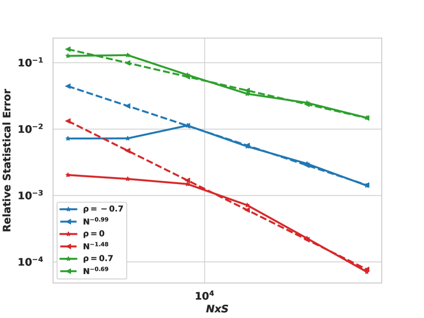
Figure 3.2: Effect of the correlation parameter, $\rho$, on the convergence of RQMC for a two-dimensional call on the minimum option under the GBM model with $S_{0}^{j}=100$, $K=100$, $r=0$, $T=1$, $\sigma_{j}=0.2$, $j=1,2$, and $\boldsymbol{C}=\begin{bmatrix}1&\rho\\ \rho&1\\ \end{bmatrix}$. For the domain transformation, $\tilde{\sigma}_{j}=\frac{1}{\sqrt{T}\sigma_{j}}=5$, where $j=1,2$. $N$: number of QMC points; $S=32$: number of digital shifts.

Case of dependent assets:

For dependent stocks, the joint characteristic function cannot be decomposed into the product of univariate characteristic functions, and

(3.7) $$\phi^{GBM}_{\boldsymbol{X}_{T}}(\boldsymbol{z}):=\operatorname{exp}\left(\mathrm{i}\boldsymbol{z}^{\prime}\left(\boldsymbol{r}-\frac{1}{2}\operatorname{diag}(\boldsymbol{\Sigma})\right)T-\frac{T}{2}\boldsymbol{z}^{\prime}\boldsymbol{\Sigma}\boldsymbol{z}\right),\boldsymbol{z}\in\mathbb{C}^{d},\Im[\boldsymbol{z}]\in\delta^{VG}_{X}.$$

Consequently, we select the proposal density $\psi^{nor}(\cdot)$ corresponding to the multivariate normal PDF, given by ψ^nor(y) = (2π)^-d2(det( ~Σ))^-12 exp(- 12(y^′ ~Σ^-1 y ) ),  y ∈R^d,   ~Σ ⪰0 where the matrix $\boldsymbol{\tilde{\Sigma}}$ may have nonzero off-diagonal components. In this case, the singularity of the integrand is controlled by the function, $r^{GBM}(\boldsymbol{u})$, defined as r^GBM(u) := ϕXT(Ψnor-1(u) + i R) ψnor( Ψnor-1(u)) ,  u ∈[0,1]^d, R ∈δ^VG_V. By substituting in the explicit expressions of the characteristic function and proposal density, we obtain the following expression for $r^{GBM}(\boldsymbol{u})$: $r^{GBM}(\boldsymbol{u})$,

(3.8) $$r^{GBM}(\boldsymbol{u}) =\underbrace{(\operatorname{det}(\boldsymbol{\tilde{\Sigma}}))^{\frac{1}{2}}\exp\left(-\frac{1}{2}(\Psi_{nor}^{-1}(\boldsymbol{u}))^{\prime}\left(T\boldsymbol{\Sigma}-\boldsymbol{\tilde{\Sigma}}^{-1}\right)(\Psi_{nor}^{-1}(\boldsymbol{u}))\right)}_{:=h_{1}^{GBM}(\boldsymbol{u})}$$

$$\times\underbrace{(2\pi)^{\frac{d}{2}}\operatorname{exp}\left(\mathrm{i}\left(\Psi_{nor}^{-1}(\boldsymbol{u})+\mathrm{i}\boldsymbol{R}\right)^{\prime}\left(\boldsymbol{r}-\frac{1}{2}\operatorname{diag}(\boldsymbol{\Sigma})\right)T+\frac{T}{2}\boldsymbol{R}^{\prime}\boldsymbol{\Sigma}\boldsymbol{R}\right)}_{:=h^{GBM}_{2}(\boldsymbol{u})}.$$

From (3.8), the function $h^{GBM}_{2}(\boldsymbol{u})$ is bounded for $\boldsymbol{u}\in[0,1]^{d}$; hence, the part controlling the boundary growth of the integrand is given by $h_{1}^{GBM}(\boldsymbol{u})$. Similarly to (3.6), we enumerate three possible limits, depending on the choice of $\boldsymbol{\tilde{\Sigma}}$:

(3.9) $$\lim_{u_{j}\to 0}h_{1}^{GBM}(\boldsymbol{u})=\left\{\begin{array}[]{l}+\infty\;\ \text{if}\;\boldsymbol{\Sigma}-\frac{1}{T}\boldsymbol{\tilde{\Sigma}}^{-1}\prec 0\;(i),\\ (\operatorname{det}(\boldsymbol{\tilde{\Sigma}}))^{\frac{1}{2}}<\infty\;\text{if}\;\boldsymbol{\tilde{\Sigma}}=\frac{1}{T}\boldsymbol{\Sigma}^{-1}\;(ii),\\ 0\;\text{if}\;\boldsymbol{\Sigma}-\frac{1}{T}\boldsymbol{\tilde{\Sigma}}^{-1}\succ 0\;(iii).\\ \end{array}\right.$$

From (3.9), an appropriate choice of the matrix $\boldsymbol{\tilde{\Sigma}}$ satisfies either Condition (ii) or (iii). However, Condition (iii) does not result in a unique choice of the matrix $\boldsymbol{\tilde{\Sigma}}$. The transformed integrand is multiplied by the factor $(\operatorname{det}(\boldsymbol{\tilde{\Sigma}}))^{\frac{1}{2}}$; thus, the aim is to select a matrix $\boldsymbol{\tilde{\Sigma}}$ to satisfy Condition (iii), with the minimum possible determinant to avoid high peaks of the integrand around the origin, which was motivated by previous findings (see [bayer2022optimal]). Optimally, the choice of $\boldsymbol{\tilde{\Sigma}}$ is given by the following constrained optimization problem:

(3.10) $$\boldsymbol{\tilde{\Sigma}}^{*} =\operatorname*{arg\,min}_{\boldsymbol{\tilde{\Sigma}}}\det(\mathbf{\tilde{\Sigma}})$$

$$\text{s.t}\;\boldsymbol{\Sigma}-\frac{1}{T}\boldsymbol{\tilde{\Sigma}}^{-1}\succeq 0$$

Instead, we propose the following construction of the matrix $\boldsymbol{\tilde{\Sigma}}$. The matrix $\boldsymbol{\Sigma}$ is real symmetric; thus, by the spectral theorem, it has an eigenvalue decomposition (EVD) (i.e., $\boldsymbol{\Sigma}=\boldsymbol{P}\boldsymbol{D}\boldsymbol{P}^{-1}$, with $\boldsymbol{D}=\operatorname{diag}(\lambda_{1},\ldots,\lambda_{d})$ and $\lambda_{j}>0,j=1,\ldots d$) because $\boldsymbol{\tilde{\Sigma}}\succ 0$. To simplify the problem in (3.10), we selected the matrix $\boldsymbol{\tilde{\Sigma}}$ to be in the form of $\boldsymbol{\tilde{\Sigma}}:=\boldsymbol{P}\boldsymbol{\tilde{D}}\boldsymbol{P}^{-1}$, where $\boldsymbol{\tilde{D}}=\operatorname{diag}(\tilde{\lambda}_{1},\ldots,\tilde{\lambda}_{d})$. In this case, we can express the constraint in (3.10) as follows: P (D - 1T ~D^-1 ) P^-1 ⪰0 ⇔~λ_j ≥1λjT,   j ∈I_d Hence, a suboptimal choice for $\boldsymbol{\tilde{\Sigma}}$ is $\boldsymbol{\tilde{\Sigma}}=\boldsymbol{P}\operatorname{diag}(\frac{1}{\lambda_{1}T},\ldots,\frac{1}{\lambda_{d}T})\boldsymbol{P}^{-1}=\frac{1}{T}\boldsymbol{\Sigma}^{-1}$, which is the choice adopted in this work.

Another challenge is the numerical evaluation of $\Psi_{nor}^{-1}(\boldsymbol{u};\boldsymbol{\tilde{\Sigma}})$, for which no closed-form expression or sufficiently fast approximation exists. To circumvent this problem, we expressed the multivariate normal RV with a zero mean and covariance matrix $\boldsymbol{\tilde{\Sigma}}$, $\mathbf{X}\sim\mathcal{N}_{d}(\mathbf{0},\boldsymbol{\tilde{\Sigma}})$, as $\mathbf{X}=\boldsymbol{\tilde{L}}\mathbf{Z}$, where $\boldsymbol{\tilde{L}}\boldsymbol{\tilde{L}}^{\prime}=\boldsymbol{\tilde{\Sigma}}$ is computed via the Cholesky decomposition of $\boldsymbol{\tilde{\Sigma}}$ or $\boldsymbol{\tilde{L}}=\boldsymbol{P}\boldsymbol{D}^{\frac{1}{2}}$. In addition, $\boldsymbol{\tilde{\Sigma}}=\boldsymbol{P}\boldsymbol{D}\boldsymbol{P}^{-1}$ is the EVD of the matrix $\boldsymbol{\tilde{\Sigma}}$, and $\mathbf{Z}\sim\mathcal{N}_{d}(\mathbf{0},\boldsymbol{I}_{d})$. Based on this representation, we obtained the following relation: $\Psi_{nor}^{-1}(\boldsymbol{u};\boldsymbol{\tilde{\Sigma}})=\boldsymbol{\tilde{L}}\Psi_{nor}^{-1}(\boldsymbol{u};\boldsymbol{I_{d}})$, where $\Psi_{nor}^{-1}(\boldsymbol{u};\boldsymbol{I_{d}})$ can be computed elementwise using the univariate ICDF. In conclusion, the option price can be obtained by approximating the following integral using RQMC:

∫_R^dg(y) dy = ∫_[0,1]^d g (~LΨnor-1(u; Id) )ψnor(~LΨnor-1(u; Id) )d u.

Figure 3.3 reveals the importance of using the general rule for the domain transformation (i.e., $\boldsymbol{\tilde{\Sigma}}=\frac{1}{T}\Sigma$) compared to the rule $\tilde{\sigma}_{j}=\frac{1}{\sqrt{T}\sigma_{j}},j=1,\ldots d$, where assets are correlated. The former rule retains the optimal convergence rate of RQMC.

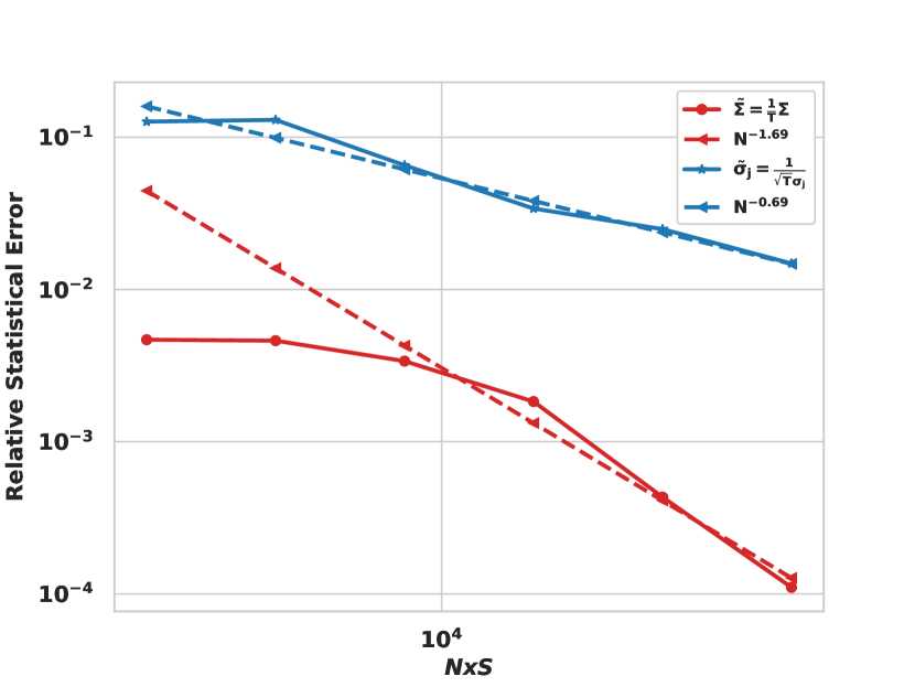
(a)

Figure 3.3: Convergence of the RQMC error for various domain transformations in the case of a two-dimensional call on the minimum option under the GBM model with $S_{0}^{j}=100$, $K=100$, $r=0$, $T=1$, $\sigma_{j}=0.2$, $j=1,2$, and $\boldsymbol{C}=\begin{bmatrix}1&0.7\\ 0.7&1\\ \end{bmatrix}$. $N$: number of QMC points; $S=32$: number of digital shifts.

Remark 3.1.

Alternative approaches to deal with the multivariate ICDF can rely on the Rosenblatt transformation [rosenblatt1952remarks], Nataf transformation [lebrun2009innovating] or the copula theory [nelsen2006introduction]. Investigating the efficiency of these alternatives is left for future work.

3.2.2 Domain transformation for the VG model

In this section we follow the same steps as in Section 3.2.1 to obtain an appropriate domain transformation for the VG model.

Case of independent assets

This section follows the same steps as in Section 3.2.1 to obtain an appropriate domain transformation for the VG model.

Case of independent assets:

We considered the case in which the underlying assets are independent; hence, the multivariate characteristic function can be factored into the product of the univariate characteristic functions, leading to the following relation:

ϕ^VG_X_T(z) = ∏_j = 1^d ϕ^VG_X_T(z_j), z ∈C^d, ℑ[ z ]∈δ^VG_X, where ϕ^VG