Are Dense Labels Always Necessary for
3D Object Detection from Point Cloud?

Abstract

Current state-of-the-art (SOTA) 3D object detection methods often require a large amount of 3D bounding box annotations for training. However, collecting such large-scale densely-supervised datasets is notoriously costly. To reduce the cumbersome data annotation process, we propose a novel sparsely-annotated framework, in which we just annotate one 3D object per scene. Such a sparse annotation strategy could significantly reduce the heavy annotation burden, while inexact and incomplete sparse supervision may severely deteriorate the detection performance. To address this issue, we develop the SS3D++ method that alternatively improves 3D detector training and confident fully-annotated scene generation in a unified learning scheme. Using sparse annotations as seeds, we progressively generate confident fully-annotated scenes based on designing a missing-annotated instance mining module and reliable background mining module. Our proposed method produces competitive results when compared with SOTA weakly-supervised methods using the same or even more annotation costs. Besides, compared with SOTA fully-supervised methods, we achieve on-par or even better performance on the KITTI dataset with about 5× less annotation cost, and 90% of their performance on the Waymo dataset with about 15× less annotation cost. The additional unlabeled training scenes could further boost the performance. The code will be available at https://github.com/gaocq/SS3D2.

Abstract

In this supplementary material, we firstly present more analysis of visualization comparison, containing different results on the KITTI dataset and the Waymo dataset for the proposed method as well as other ones. Besides, we provide more analysis of pseudo instances to comprehensively explore the influences. Finally, we demonstrate the algorithm of the learning process from streaming unlabeled scenes to ease the reproduction of the proposed method.

1 Introduction

Autonomous driving, which aims to enable vehicles to perceive the surrounding environments intelligently and move safely with little or no human effort, has attracted much attention recently [16]. As one of the fundamental problems in autonomous driving, detecting 3D objects accurately from a point cloud is crucial for real-world applications. With the advances of deep learning techniques in computer vision and robotics, a number of approaches [14, 23, 15, 12, 28] based on either voxel-wise or point-wise features have been proposed and achieved state-of-the-art (SOTA) performance on large-scale benchmark datasets [13, 9].

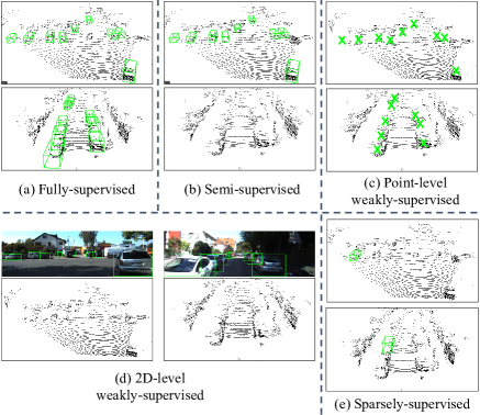
Figure 1: Illustration of annotation setup for different supervision forms. The green boxes represent 3D or 2D box annotations and the green crosses represent point-level center annotations in the BEV point cloud map. In this paper, we explore a sparse annotation setup in which we just annotate one 3D object in each scene, as shown in Fig. (e).

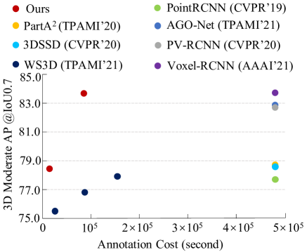
Figure 2: Illustration of 3D moderate AP (Average Precision) vs. annotation cost, tested on KITTI  [13] validation set and the AP is calculated with 11 recall positions at IoU 0.7 for the car to compare with the previous methods. Compared with SOTA fully-supervised detectors, our SS3D++ yields promising results with a far lower annotation demand. Besides, when providing less annotations than the remarkably weakly-supervised WS3D [24], our SS3D++ still shows profitable detection performance.

However, most of the proposed 3D object detectors require large-scale, precisely densely-annotated datasets. Unfortunately, collecting high-quality 3D annotations is often time-consuming and labor-intensive compared with 2D image object annotations, in which annotators have to switch viewpoints or zoom in and out throughout a 3D scene carefully for annotating each 3D object, and take hundreds of hours to annotate just one hour of driving data [24]. This poses a huge challenge faced by 3D object detection systems in real-world settings, which requires massive, exhaustively-labeled 3D densely-supervised training data. Therefore, in order to promote the deployment of current 3D object detection systems, it is necessary and significant to reduce the cumbersome data annotation process, and meanwhile achieve 3D object detectors with on-par fully-supervised detection performance.

To mitigate this challenge, some weakly-supervised and semi-supervised approaches [59, 24, 11, 60] have been proposed, which attempt to learn 3D object detection from relatively easily acquired annotations, e.g, leveraging a few high-quality labeled and much unlabeled data [11], center-click point annotation [24] or 2D image-level bounding box annotation [59], as depicted in Fig. 1. Though these methods have substantially reduced the heavy data annotation burden, there exist several deficiencies for applying them in practice. On the one hand, as shown in Fig. 2, their performances have a large margin deterioration compared with the SOTA results of fully-supervised methods. Such dissatisfied performances would not meet the requirements for autonomous driving and practical applications. On the other hand, these low-cost annotations are hardly directly trained using current SOTA fully-supervised detectors, e.g., WS3D [24] need to additionally elaborately designed detector architecture, 3DIoUMatch [11] needs to use additive IoU-estimation module to predict 3D IoU value. These specific detector designs for various weakly-supervised forms relatively restrict the potential to benefit from up-to-date SOTA fully-supervised 3D detectors. Both of the above two aspects may prevent the applicability of these weakly-supervised approaches in real-world settings.

To further promote the deployment of 3D object detection systems, in this paper, we propose a novel sparsely-supervised method that learns 3D object detectors from sparse annotation data in which we just annotate one 3D object per scene, as illustrated in Fig. 1. Intuitively, such novel weakly-supervised annotation form facilitates learning information of unlabeled objects, since infra-scene information transfer is much easier than cross-scene information transfer. Comparatively, semi-supervised scenario [11] may fall into the suboptimal solution due to limited information transfer from labeled to large discrepancy unlabeled scenes, and existing weakly-supervised scenarios may suffer intractable location issues due to significant disparity between 2D-level [59] or point-level [24] weak annotations and 3D-level annotations. Therefore, the proposed sparse annotation strategy has the potential to achieve better performance.

However, such sparsely annotated training data provides inexact and incomplete supervision, naturally raising several new challenges. (1) The missing-annotated instances and the region near those instances may be incorrectly marked as background, which can easily deteriorate the detector under the guidance of incorrect negative samples; (2) To eliminate the negative effect of inexact supervision from positive samples, we are required to generate reliable pseudo-annotated instances (high precision), and find possibly many newly annotated instances (high recall); (3) The sparsely-annotated object in each scene is randomly chosen, while the hardness of learning different objects has great differences. This possibly hinders the knowledge transfer from labeled objects to unlabeled objects, and thus impairs the performance on unlabeled instances.

To address these challenges, we propose a novel and effective method for sparsely annotated 3D object detection, namely SS3D++, which can be applied to any existing off-the-shelf fully-supervised 3D detectors. The main idea of our SS3D++ is to progressively mine positive instances and backgrounds with high confidence using the proposed reliable background mining module and missing-annotated instance mining module, and further use them to generate confident fully-annotated scenes by the GT (ground-truth) Sampling [10] data augmentation strategy. Such a strategy could guarantee that generated pseudo annotations of training instances with high recall provide sufficient knowledge for training the 3D detector. By leveraging the mutual amelioration between high-quality training scene generation and 3D detector training, compared with the 3D detector trained with the fully annotated dataset, our SS3D++ can achieve comparable or even better performance on the KITTI dataset [13] with $5\times$ less annotations, and obtain 90% performance with $15\times$ less annotations on the Waymo dataset [9].

Our sparsely-supervised framework has three appealing characteristics. First, we can achieve high performance approaching or even surpassing SOTA fully-supervised methods, as presented in Table I and Table III about experimental results of the KITTI [13] and Waymo datasets [9]. However, we only require $5\times$ less annotations than fully-supervised methods on KITTI dataset [13], as shown in Fig. 2. Besides, our annotation cost is similar or even less than existing weakly-supervised approaches [59, 24, 11]. Specifically, under the similar number of 3D annotation objects, our annotations are relatively more easily acquired than existing weakly-supervised methods, since it is often easy to just annotate one 3D object per scene. Comparatively, 3DIoUMatch [11] needs to annotate dense 3D objects traversing the entire scene, and WS3D [24] needs to additionally provide center-click point annotations for each 3D object in the entire training scene data. Despite its simplicity in annotation manner, our SS3D++ method is able to achieve substantially better performance, and tends to bridge the performance gap between weakly-supervised learning and strong fully-supervised learning. The detailed experimental results can refer to Fig. 11 and Table IV.

Second, our method is detector-agnostic, which can easily benefit from advanced fully-supervised 3D detectors. As illustrated in Tables I and III, we directly use several existing off-the-shelf advanced fully-supervised 3D detectors to train with sparsely annotated data, resulting in a severe deterioration of the detection performance. While we instantiate our SS3D++ framework as these off-the-shelf fully-supervised 3D detectors without modifying the architectures of the detectors, which consistently improves the performance approaching or even surpassing the fully-supervised results. This property is promising to apply our framework into the autonomous driving system, since it is simple and convenient to adapt to up-to-date 3D detectors and refresh the system to obtain better performance. However, existing weakly-supervised methods [59, 24, 11] elaborately designing specific architectures of detectors to address such imperfect information, relatively hardly benefit from advanced fully-supervised 3D detectors.

Third, our SS3D++ method is hopeful to learn from additional unlabeled training scenes. On the one hand, if we have access to additional unlabeled training scenes in an offline manner, as presented in Fig. 11, we can further boost the performance of a 3D detector by making use of these unlabeled data without additional annotation costs. This implies that our method is capable of generating confident pseudo annotations for easily obtained unlabeled point cloud scenes. On the other hand, if additional unlabeled training scenes arrive in an online manner, we can also continuously improve the performance of the 3D detector by making use of these streaming unlabeled data, as shown in Fig. 15 (c). This property is potentially useful for autonomous driving system, which is required to perceive the changing environment and incrementally improve itself.

This work builds upon our conference paper [52] and expands it in various aspects. Firstly, we introduce the hardness of learning different objects to eliminate the influence of randomly selecting a sparse-annotated object in a scene in Section 4.2.1. Secondly, we rigorously formulate the missing positive instances mining process as a multi-criteria sample selection process, and use sample selection curriculum setups to help to adaptively determine high-confidence positive instances involved in the training pool in Section 4.2. Thirdly, we improve the previous algorithm by leveraging the mutual benefit between 3D detector training and confident fully-annotated scene generation in Section 4.4. Fourthly, extensive ablation studies (see Sections 5.5 and 5.7) and experiments on large-scale Waymo Open Dataset (see Table III) are conducted to demonstrate the effectiveness and universality of our method. Fifthly, we make an in-depth comparison with other weakly-supervised methods in Section 5.4. Finally, we show that the proposed method has the potential for utilizing additional unlabeled training scenes to ameliorate the model in Section 5.6.

2 Related Work

Fully-supervised 3D object detection. The existing 3D detection methods can be broadly categorized into two types: voxel-based methods [10, 12, 28, 27, 33, 65] and point-based methods [64, 29, 25, 20, 32, 30]. Thanks to the seminal PointNet series [34, 36], point-based methods directly take the raw irregular points as input to extract local and global features. PointRCNN [14] directly generated 3D proposals from raw points in a bottom-up manner. Part-A² [15] further improved the PointRCNN by exploring the rich information in intra-object part locations. For voxel-based methods, voxelization is a common measure for irregular point clouds to apply traditional 2D or 3D convolution. PV-RCNN [6] extended the SECOND [10] by leveraging a keypoints branch to learn discriminative features. PV-RCNN++ [56] proposed the VectorPool aggregation module and sectorized keypoints sampling strategy to further enhance the PV-RCNN. Voxel-RCNN [23] achieved a careful balance between performance and efficiency based on the voxel representations. CenterPoint [63] firstly used a keypoint detector to detect centers of objects and then regressed to other attributes.

Prior works have made significant progress and achieved impressive performance, while these results deeply depend on the large-scale manually precisely densely-annotated 3D data, which are time-consuming and labor-intensive. We make an attempt towards weakly supervised 3D object detection considering the sparse annotation strategy which just annotates one object per scene. This enables a much faster and easier data labeling process compared to notoriously densely full supervision, and we can achieve comparable or better performance. Moreover, our method is detector-agnostic, which can easily benefit from advanced fully-supervised voxel-based or point-based detectors. We will instantiate the SS3D++ as above fully-supervised 3D detectors to demonstrate the effectiveness of our method in the experimental section.

Weakly/Semi-supervised 3D object detection. To reduce annotations of 3D objects, the weakly-supervised learning strategy is adopted in WS3D [24], which is achieved by a two-stage architecture based on the click-annotated scheme. WS3D[24] generated cylindrical object proposals by click-annotated scenes in stage-1 and refined the proposals to get cuboids using slight well-labeled instances in stage-2. However, the supervision information provided by the weakly-supervised point annotation is too weak, so that a certain amount of full annotations have to be provided additionally. Meanwhile, some semi-supervised methods [26, 67, 66, 68] leveraged the mutual teacher-student framework to transfer information from labeled scenes to unlabeled scenes. 3DIoUMatch [11] conducted a pioneering work for outdoor scenes, which estimate 3D IoU as a localization metric and set a self-adjusted threshold to filter pseudo labels. Though these methods have substantially reduce the heavy data annotation burden, they have a large margin performance gap with fully-supervised methods, and relatively hardly benefit from advanced 3D detectors. All of these prevent potential practical applicability of 3D object detection. In this paper, we attempt to explore a new weakly-supervised form, sparse supervision, and facilitate 3D object detection close to practical applications.

Sparsely-supervised 2D object detection. Due to that a part of instances are missing-annotated, weight updated of the network may be misguided significantly when gradients back-propagated. To address this issue, existing 2D detection methods employed re-weight or re-calibrates strategy on the loss of RoIs (regions of interest) to eliminate the effect of unlabeled instances. Soft sampling [21] utilized overlaps between RoIs and annotated instances to re-weight the loss. Background recalibration loss[18] based on focal loss[7] regarded the unlabeled instances as hard-negative samples and re-calibrates their losses, which is only applicable to single-stage detectors. Especially, part-aware sampling[19] ignored the classification loss for part categories by using human intuition for the hierarchical relation between labeled and unlabeled instances. Co-mining [17] proposed a co-generation module to convert the unlabeled instances as positive supervisions. However, these sparsely annotated object detection methods are all for 2D image objects. Due to the modal difference between 2D images and 3D point cloud, these methods can not be directly applied to our 3D object detection task. For example, in KITTI [13], 3D objects are naturally separated, which means the overlaps among objects are zero and the hierarchical relation between objects does not exist. Compare with the re-weight and re-calibrates methods, in this paper, we propose a novel method for sparsely annotated 3D object detection which leverages a simple but effective background mining module and a missing-annotated instance mining module to mine confident positive instances and backgrounds, which is key for training detectors with high performance.

Curriculum learning for object detection. Curriculum learning [37, 43, 47] is a training strategy that trains a machine learning model in a meaningful order, demonstrating that learning from easy to hard examples can be beneficial. This strategy has been successfully employed in object detection[38, 39, 48, 49, 51, 55, 54]. [38] proposed a curriculum learning strategy to feed training images into the weakly supervised object localization learning loop in an order from images containing bigger objects down to smaller ones. Based on [50], C-SPCL[49] proposed a novel collaborative self-paced curriculum learning framework for weakly supervised object detection, which combined the instance-level confidence inference, the image-level confidence inference, and the self-paced learning mechanism to increase the learning robustness. Under very few annotated samples, [58] embedded multi-modal learning and curriculum learning to ameliorate the trade-off between precision and recall in training data production. Different from these methods tackling 2D object detection, we explore curriculum learning to 3D object detection.

Our proposed method also is inspired by self-paced learning (SPL) [53], so we provide a brief overview here. Let $\mathcal{D}=\left\{x_{i},y_{i}\right\}_{i=1}^{N}$ indicates the training set, where $x_{i}$ and $y_{i}$ denote the feature and label of sample $i$, respectively. The model $f$ with weight parameters $\phi$ map each $x_{i}$ to the prediction $f(x_{i},\phi)$, and $l_{i}=L(f(x_{i},\phi),y_{i})$ denotes the loss, where $L$ is the learning objective. Then the goal is to minimize the loss on the whole training set:

$$\min_{\phi;\boldsymbol{v}\in[0,1]^{N}}\mathbb{E}(\phi,\boldsymbol{v};\lambda)=\sum_{i=1}^{N}v_{i}l_{i}-\lambda\sum_{i=1}^{N}v_{i},$$ (1)

where $\lambda$ is the age parameter for controlling the learning pace, and $\boldsymbol{v}=\left[v_{1},v_{2},\ldots,v_{N}\right]^{\top}\in[0,1]^{N}$ is the latent weight variable. The above learning objective is generally optimized with ACS (Alternative Convex Search) [50]. Concretely, it alternatively optimize $\phi$ and $\boldsymbol{v}$ while fixing the other. With the fixed $\boldsymbol{v}$, the global optimum $\phi^{*}$ can be learned by the existing off-the-shelf supervised learning. Then, with fixed $\phi$, the close-formed optimal solution for $\boldsymbol{v}^{*}$ can be obtained by solving:

$$v_{i}^{*}=\left\{\begin{array}[]{lr}1,&l_{i}<\lambda,\\ 0,&\text{ otherwise. }\end{array}\right.$$ (4)

This solution exists an intuitive explanation: if a sample has a loss $l_{i}$ less than the threshold $\lambda$, then it is taken as an easy sample for the current model, and will be selected in training (i.e., $v_{i}^{*}=1$). Otherwise, it is hard and unselected (i.e., $v_{i}^{*}=0$). Initially, $\lambda$ should be set suitable to ensure that a small proportion of easy sample are selected. When the model becomes more mature, $\lambda$ should grow and more harder samples get involved in the training process.

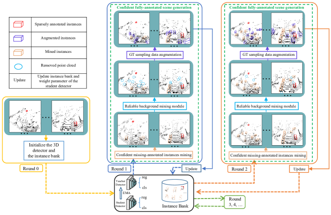
Figure 3: The pipeline of our SS3D++ algorithm. We alternatively improve 3D detector training and confident fully-annotated scene generation in a unified learning scheme. To efficiently train the 3D detector, we construct confident fully-annotated scenes based on the missing-annotated instance mining module, the reliable background mining module , and the GT sampling data augmentation strategy. By leveraging the mutual amelioration between high-quality training scene generation and 3D detector training, the obtained 3D detector becomes more robust and well-performing.

3 Preliminaries

3.1 3D Object Detector and Notation

In this paper, we focus on the 3D object detection in autonomous driving scenarios which aims to predict the attributes of 3D objects from point cloud inputs. Formally, we denote the 3D object detector model as $F$, and the 3D object detection task can be formulated as

$$E_{i}=F(P_{i};\phi),i=1,\cdots,M,$$ (5)

where $E_{i}=\{E_{ij}\},j=1,\cdots,N_{i}$ is a set of detected 3D objects in the $i$-th scene with an input scene $P_{i}\in\mathbb{R}^{N\times 3}$ containing $N$ points, $\phi$ is the weight parameter of $F$, $M$ is the total number of point cloud scenes in the dataset, and $E_{ij}$ can be written as

$$E_{ij}=(r,p),r=[x,y,z,l,w,h,\theta],$$ (6)

where $r$ is the 3D bounding box and $p$ denotes the predicted probability of belonging to the class $c$. In this paper, we consider a 3D bounding box represented in the LiDAR coordinate system, in which $(x,y,z)$ is the 3D center coordinate , $(l,w,h)$ is the length, width, and height of a cuboid, respectively, and $\theta$ is the orientation from the bird’s view.

3.2 Fully-Supervised 3D Object Detection

Considering the fully-supervised setting, it is often given a training dataset $\mathcal{D}=\{(P_{1},G_{1}),\ldots,(P_{M},G_{M})\}$ and the corresponding ground-truth, where $G_{i}=\left\{\left(b_{ij},y_{ij}\right)\right\},j=1,\cdots,N_{i}$, and for each $(b_{ij},y_{ij})$, $b_{ij}$ is the oriented 3D bounding box of the $j$-th object instance in a point cloud scene $P_{i}$, and $y_{ij}\in\{1,\ldots,C\}$ is the class label. Based on the training dataset $\mathcal{D}$, the 3D object detector model $F$ can be learned by the following loss function

$$\mathcal{L}_{F}=\mathcal{L}_{cls}+\mathcal{L}_{reg},$$ (7)

where classification loss $\mathcal{L}_{cls}$ is used to learn the classifier to predict the category of a 3D object, and $\mathcal{L}_{reg}$ is utilized to learn the location, size and heading angle of the 3D object. If we take the proposal-based two-stage 3D detector Voxel-RCNN [23] as an example, the Eq. (7) degenerates as

$$\mathcal{L}_{F}=\mathcal{L}_{cls}^{RPN}+\mathcal{L}_{reg}^{RPN}+\mathcal{L}_{cls}^{Head}+\mathcal{L}_{reg}^{Head},$$ (8)

where $\mathcal{L}_{cls}^{RPN}$ is the Focal Loss [7] for classification in the region proposal network (RPN) stage, $\mathcal{L}_{cls}^{Head}$ is the Binary Cross Entropy Loss for confidence prediction in the detection head stage, and Huber Loss is exploited in $\mathcal{L}_{reg}^{RPN}$ and $\mathcal{L}_{reg}^{Head}$ for box regression.

4 Sparsely-Supervised 3D Object Detection Framework and Learning Algorithm

Though fully-supervised 3D object detection obtains impressive performance, they require large-scale, precisely densely-annotated 3D training data. This data collection process is quite time-consuming and labor-intensive, which prevents the potential applicability of 3D object detection in real-world settings. In this work, we study the following sparsely annotated 3D object detection setting, i.e., we have only access to one 3D bounding box annotation $\tilde{G}_{i}=\{(b_{i1},y_{i1})\}$ for any scene $P_{i}$, and the annotations of remaining object instances are missing. Such inexact and incomplete supervision greatly saves annotation efforts. In contrast to prior weakly-supervised attempts [59, 24, 11] (as shown in Fig. 1), our novel sparse supervision form introduces more potential practical and commercial benefits, while bringing some new challenges (please refer to Section 1). In this section, we will present the proposed SS3D++ method to address these challenges.

4.1 Overview SS3D++ Framework and Modeling

We aim to facilitate the learning strategy of a 3D detector to obtain the optimal detection performance when training from scratch on the sparsely annotated dataset $\tilde{\mathcal{D}}=\{(P_{1},\tilde{G}_{1}),\ldots,(P_{M},\tilde{G}_{M})\}$. However, such sparsely annotated data provides inexact and incomplete supervision, inevitably raising the severe deterioration of fully-supervised 3D detectors, as shown in Tables I and III.

To reduce the negative influence of inexact and incomplete supervised information, it is encouraged to generate pseudo annotations for those missing-annotated instances. Without loss of generality, we consider the formulation for the $i$-th scene, which can be easily applied to all training scenes by cancelling out the index $i$. Note that the use of $i$ is for the easy clarity, the actual optimization is carried out through minibatch. To mine more confident missing-annotated positive samples, we propose to use a meaningful multi-criteria sample selection curriculum (Eqs. (11), (12), and (13)), and further improve the 3D detector using the selected positive instances in Eq. (10). To sum up, our approach can be formulated as the following optimization objective:

$$\ \mathbf{u}_{i}^{*},\mathbf{v}_{i}^{*},\mathbf{k}_{i}^{*} =\mathop{\arg\min}_{\mathbf{u}_{i},\mathbf{v}_{i},\mathbf{k}_{i}}\mathcal{E}(\mathbf{u}_{i},\mathbf{v}_{i},\mathbf{k}_{i};\phi^{*},\lambda)$$

$$\triangleq\mathcal{L}_{c\lambda}+\mathcal{L}_{r\lambda}+\mathcal{L}_{d\lambda},$$ (9)

$$\phi^{*},\tilde{U}_{i}^{*}=\mathop{\arg\min}_{\phi,\tilde{U}_{i}}\mathcal{E}(\phi,\tilde{U}_{i};\mathbf{u}_{i}^{*},\mathbf{v}_{i}^{*},\mathbf{k}_{i}^{*})\triangleq\mathcal{L}_{s}+\mathcal{L}_{p},$$ (10)

where

$$\mathcal{L}_{c\lambda}=\sum_{j=2}^{N_{i}}\sum_{c=1}^{C}u_{ijc}\mathcal{L}^{c}_{cls}(p_{ij}(\phi^{*}),\tilde{y}_{ij}^{*})-\sum_{j=2}^{N_{i}}\sum_{c=1}^{C}\lambda^{u}_{ic}u_{ijc},$$ (11)

$$\mathcal{L}_{r\lambda}=\sum_{j=2}^{N_{i}}\sum_{c=1}^{C}v_{ijc}\mathcal{L}^{c}_{reg}(\mathcal{A}(r_{ij}(\phi^{*})),\tilde{r}_{ij})-\sum_{j=2}^{N_{i}}\sum_{c=1}^{C}\lambda^{v}_{ic}v_{ijc},$$ (12)

$$\mathcal{L}_{d\lambda}=\sum_{j=2}^{N_{i}}\sum_{c=1}^{C}k_{ijc}d^{c}(r_{ij}(\phi^{*}))-\sum_{j=2}^{N_{i}}\sum_{c=1}^{C}\lambda^{k}_{ic}k_{ijc},$$ (13)

denote three different curriculum learning objectives,

$$\mathcal{L}_{s}=\mathcal{L}_{F}(E_{i1}(\phi),\tilde{G}_{i1}),$$ (14)

$$\mathcal{L}_{p}=\sum_{j=2}^{N_{i}}\sum_{c=1}^{C}u_{ijc}v_{ijc}k_{ijc}\mathcal{L}^{c}_{F}(E_{ij}(\phi),\tilde{U}_{ij}),$$ (15)

are the loss for sparse annotation and pseudo instances, respectively, $\tilde{G}_{i1}=(b_{i1},y_{i1})$ is the given sparse supervision of the $i$-th scene, $\tilde{U}_{ij}=(\tilde{b}_{ij},\tilde{y}_{ij})$ and $\tilde{U}_{i}^{*}$ represent the previously generated pseudo instances and the currently generated pseudo instances, respectively, while $\tilde{b}_{ij}$ and $\tilde{y}_{ij}$ are bounding boxes and class prediction for the mined $j$-th positive instance, respectively. $\phi$ is the weight parameter of detector $F$, which can be instantiated as any existing off-the-shelf fully-supervised 3D object detectors (please see Section 5). $u_{ijc},v_{ijc},k_{ijc}\in\{0,1\}$ are the learnable sample selection variables encoding whether the detected result in the $i$-th scene are determined as reliable positive instances to further train the detector, and $\mathbf{u}_{i},\mathbf{v}_{i},\mathbf{k}_{i}$ are weight matrix, $\mathbf{u}_{i},\mathbf{v}_{i},\mathbf{k}_{i}\in\{0,1\}^{(N_{i}-1)\times C}$, denoting the collection of the selection variables $u_{ijc},v_{ijc},k_{ijc}$ for all mined positive instances with different class $c$. $\lambda^{u}_{ic},\lambda^{v}_{ic},\lambda^{k}_{ic}$ are the hyperparameter for the SPL regularization term [53, 42], which enables the possible selection of high-confidence images during optimization. $r_{ij},\tilde{r}_{ij}$ are the predicted bounding boxes of the detector $F$ by inputting scenes $P_{i}$ and $\mathcal{A}(P_{i})$, respectively, where $\mathcal{A}(\cdot)$ is a set of global augmentation strategies including random rotation, flipping, and scaling. $d(r_{ij}(\phi))$ represents the reciprocal of the density estimation of the predicted bounding boxes $r_{ij}$ by the detector $F(\cdot,(\phi))$, which is the cardinality of $S_{ij}$, i.e., the number of the points inside the 3D bounding box.

Actually, above formation is a bi-level optimization objective [40]. Calculating the optimal detector $F$ in the inner-loop can be very expensive. This motivates us to adopt online iterative updation by the sequence $\phi,\tilde{U}_{i},\mathbf{u}_{i},\mathbf{v}_{i},\mathbf{k}_{i}$, until the maximum iteration round number is reached. Next we show how to solve each parameter as follows.

Update $\mathbf{u}_{i},\mathbf{v}_{i},\mathbf{k}_{i}$. For each training iteration, we can obtain $\mathbf{u}_{i},\mathbf{v}_{i},\mathbf{k}_{i}$ for the $i$-th scene by solving Eqs. (11), (12), and (13) based on last step $\phi^{(t)}$ and $\tilde{U}_{i}^{(t)}$. Then the closed-form solution is

$$u^{(t+1)}_{ijc} =\left\{\begin{array}[]{ll}1&\mathcal{L}^{c}_{cls}(p_{ij},y_{ij}^{(t)};\phi^{(t)})<\lambda^{u}_{ic}\\ 0&\mathcal{L}^{c}_{cls}(p_{ij},y_{ij}^{(t)};\phi^{(t)})\geq\lambda^{u}_{ic}\end{array},\right.$$ (18)

$$v^{(t+1)}_{ijc} =\left\{\begin{array}[]{ll}1&\mathcal{L}^{c}_{reg}(\mathcal{A}(r_{ij}),\tilde{r}_{ij};\phi^{(t)})<\lambda^{v}_{ic}\\ 0&\mathcal{L}^{c}_{reg}(\mathcal{A}(r_{ij}),\tilde{r}_{ij};\phi^{(t)})\geq\lambda^{v}_{ic}\end{array},\right.$$ (21)

$$k^{(t+1)}_{ijc} =\left\{\begin{array}[]{ll}1&d^{c}(r_{ij};\phi^{(t)})<\lambda^{k}_{ic}\\ 0&d^{c}(r_{ij};\phi^{(t)})\geq\lambda^{k}_{ic}\end{array},\right.$$ (24)

and the implementation details of this multi-criteria sample selection process can be refer to Section 4.2.

Update $\tilde{U}_{i}$. The next step is to update pseudo instances $\tilde{U}_{i}$ of the training scene $P_{i}$ by solving the following minimization sub-problem:

$$\tilde{U}_{i}^{*}=\mathop{\arg\min}_{\tilde{U}_{i}}\mathcal{L}_{p}.$$ (25)

It is easy to see that the global optimum of the above problem can be obtained by directly setting the pseudo annotations equal to the predictions of the detector. Here, we adopt teacher network with EMA predictions for each of the training instances to generate high quality of pseudo annotations $\tilde{U}_{i}^{(t+1)}$, which is the commonly used technique in semi-supervised learning [46].

Update $\phi$. Finally, we train the 3D object detector given $\mathbf{u}^{(t+1)}_{i},\mathbf{v}^{(t+1)}_{i},\mathbf{k}^{(t+1)}_{i}$ and $\tilde{U}_{i}^{(t+1)}$. Specifically, after obtaining pseudo instances from the teacher detector, we can formulate the loss of student detector as follows:

$${\phi}_{s}^{*}=\mathop{\arg\min}_{{\phi}}(\mathcal{L}_{s}+\mathcal{L}_{p}).$$ (26)

Then, the the weight parameter $\phi_{s}$ of the student detector is updated via stochastic gradient descent:

$$\phi_{s}\leftarrow\phi_{s}-\gamma\frac{\partial(\mathcal{L}_{s}+\mathcal{L}_{p})}{\partial\phi_{s}},$$ (27)

where $\gamma$ is the learning rate. Next, we apply the effective EMA [46] approach which has been shown to be effective in many existing works to update the learned weight $\phi_{m}$ of the teacher detector as follows:

$$\phi_{m}\leftarrow\alpha\phi_{m}+(1-\alpha)\phi_{s},$$ (28)

where $\alpha$ is the EMA coefficient. Note that the training data are the union set of initial sparse annotated instances and selected instances ($u_{ij}=v_{ij}=k_{ij}=1$) with the pseudo annotation $\tilde{U}_{i}$. To increase the learning efficiency of the detector, we further generate confident fully-annotated scenes based on the mined reliable background and confident missing-annotated instances. The details can refer to Section 4.4. Thus, this step can be solved by the existing standard off-the-shelf 3D object detector, described as PointRCNN [14], Part-A²[15], PV-RCNN[6], Voxel-RCNN[23], etc.

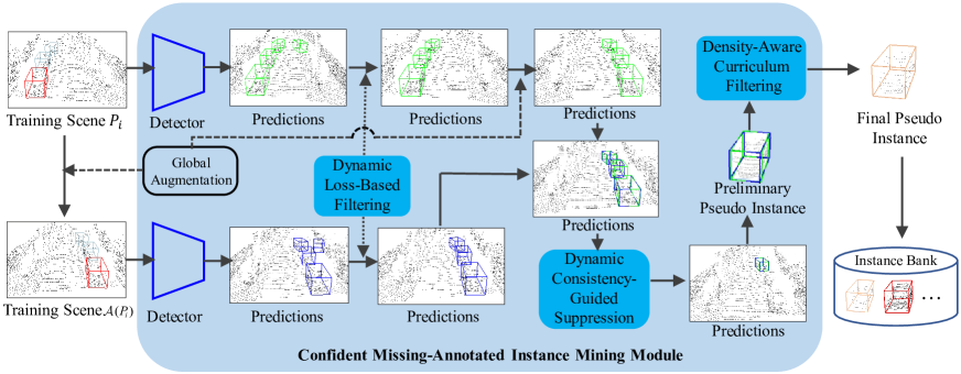
Figure 4: Illustration of proposed confident missing-annotated instance mining module. The scene $P_{i}$ and the corresponding augmented scene $\mathcal{A}({P}_{i})$ are input into the 3D detector. Then we leverage the dynamic loss-based filtering to remove the predictions of $P_{i}$ and $\mathcal{A}({P}_{i})$ with a low confidence score (i.e., large classification loss). Further, the dynamic consistency-guided suppression is proposed to filter out low-quality predictions. Lastly, we carry out the density-aware curriculum filtering process and store the remaining predictions into the instance bank as confident pseudo instances.

Algorithm 1 Algorithm of Our SS3D++ Method.

0:  Teacher detector $F_{m}$, student detector $F_{s}$, total rounds $\mathcal{T}$, instance bank ${\mathcal{B}}$, sparsely annotated dataset $\tilde{\mathcal{D}}$, global augmentation strategies $\mathcal{A}$;

1:  Initialize the instance bank ${\mathcal{B}}^{(0)}$ with given sparse annotations;

2:  Pre-train $F_{m}$ with dataset $\tilde{\mathcal{D}}$ via Eq. (7), and initialize the $F_{s}$ with the same pre-trained weight parameters;

3:  Get initial density vector $d_{0}$ via Eq. (30) in Section 4.2.2;

4:  for  $t=1$ to $\mathcal{T}$  do

5:     if $t$ >$1$ then

6:        Perform multi-criteria sample selection curriculums via Eqs. (18), (21), and (24);

7:        Using $F_{m}$ to generate pseudo instances $\tilde{U}_{i}$ via Eq. (25) and updating instance bank ${\mathcal{B}^{(t)}}$;

8:     end if

9:     Perform reliable background mining process (Algorithm 3) via the $F_{m}$ to obtain broken scene set $\tilde{P}^{(t)}$ with reliable background;

10:     while detector not converge do

11:        Perform confident fully-annotated scene generation to get $\tilde{\mathcal{D}_{c}}^{(t)}$ based on $\tilde{P}^{(t)}$ and ${\mathcal{B}^{(t)}}$;

12:        Train $F_{s}$ via Eq. (27) based on $\tilde{\mathcal{D}_{c}}^{(t)}$;

13:        Update $F_{m}$ via Eq. (28);

14:     end while

15:  end for

15:  Learned student detector $F_{s}$.

With the above analysis, it is clear to see that our approach aims to automatically select confident instances for generating pseudo instances (i.e., Eqs. (18), (21), and (24)) , and update the weight parameter $\phi$ in the above formulation with an iteratively-learning manner. The overall algorithm of our SS3D++ algorithm for sparsely-supervised 3D object detection framework is shown in Algorithm 1. Given a 3D teacher detector, initially, we train the detector from the scratch on the sparsely annotated dataset $\tilde{\mathcal{D}}$ (i.e., step 2). To increase the diversity of training data and eliminate the negative impact of missing-annotated instances, we leverage the teacher detector to mine reliable missing-annotated instances in a meaningful curriculum learning order through the missing-annotated instance mining module with strict multi-criteria sample selection curriculums through Eqs. (18), (21), and (24) (step 6, refer to Algorithm 2 and Fig. 4). Furthermore, we add the mined high quality missing-annotated instances into the instance bank. Then, we use the teacher detector to get the broken scene with mined reliable background through the reliable background mining module (details can refer to Algorithm 3 and Fig. 7), which aims to further prevent missing-annotated instances and the region near those instances from being mistaken as background. To efficiently train the student detector with sufficient knowledge, we further construct confident fully-annotated scenes based on the mined reliable background and confident missing-annotated instances (step 11, refer Section 4.4 for details). By this iteratively learning style of reliable background mining, confident missing-annotated instances mining, confident fully-annotated scene generation, and detector updating through Eqs. (27) and (28), more confident fully-annotated scenes are obtained, and the teacher/student detector becomes more robust and well-performing.

4.2 Confident Missing-Annotated Instances Mining

In this section, we detailedly illustrate the multi-criteria sample selection curriculums in Eqs. (18), (21), and (24). We implement these curriculums via a confident missing-annotated instance mining module, shown in Fig. 4, to effectively mine missing-annotated instances for each scene. Specifically, the collectively choosing process of confident instances is influenced by three critical mechanisms: dynamic loss-based filtering, dynamic consistency-guided suppression, and density-aware curriculum filtering. Then the updating equation of the pseudo instances can be formulated by updating $\mathbf{u}_{i}$, $\mathbf{v}_{i}$, and $\mathbf{k}_{i}$ along the iteratively learning process.

Next, we will delve into the detailed explanation of the multi-criteria sample selection process and corresponding adaptive sample selection curriculum setups, thereby fundamentally comprehending the origins of the three variables: $\mathbf{u}_{i}$, $\mathbf{v}_{i}$ and $\mathbf{k}_{i}$.

4.2.1 Multi-Criteria Sample Selection Process

As shown in Fig. 4, it can be seen that three selection variables $\mathbf{u}_{i},\mathbf{v}_{i},\mathbf{k}_{i}$ play distinct roles, which correspond to the following three-criteria sample selection curriculums.

• Dynamic loss-based filtering. Eq. (18) tries to filter out samples with large classification loss, which means that we tend to select instances with high-confident prediction. Along with the amelioration of detector, more high-confident prediction gradually involves in training to further boost the detector.

• Dynamic consistency-guided suppression. Inspired by the consistency-based semi-supervised learning [35], we further require that the generated bounding boxes should have fine consistency property. Specifically, we compute the mismatch between the prediction $\tilde{r}_{ij}$ of the augmented input scene and the augmented prediction $\mathcal{A}(r_{ij})$ under a same global augmentation strategy $\mathcal{A}$. As demonstrated in Eq. (21), we suppress the effect of low consistent predictions (i.e., large regression loss) during the training process, which helps to reduce the effect of noisy bounding boxes, and thus improve the performance of the detector.

• Density-aware curriculum filtering. As shown in Fig. 5, due to the occlusion, truncation and the distance from the LiDAR sensor, the objects possess different densities. The lower density of objects may contain less spatial information, which may make detector hard to extract fine features at the initial training stage. To this goal, we mine the confident objects by considering the hardness of learning different objects. Specifically, we use Eq. (24) to progressively select mined instances from easier objects (high density) to harder objects (low density) during the training process. The density $d(r_{ij}(\phi^{(t)}))$ of generated bounding boxes $r_{ij}$ can be computed using the cardinality of $S_{ij}$. Through controlling the instances involving in training from “easy” to “hard” order in terms of the density, we can obtain a more robust detector with these newly generated annotated training data.

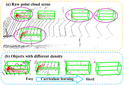
Figure 5: (a) Illustration of learning hardness (i.e., density) of different 3D objects on the KITTI dataset. (b) We select mined 3D objects in a meaningful order from “easy” to “hard”. The red represents the foreground points and the green represents the ground-truth bounding boxes.

4.2.2 Adaptive Sample Selection Curriculum Setups

Note that hyperparameters $\lambda^{u}_{ic},\lambda^{v}_{ic},\lambda^{k}_{ic}$ in Eqs. (18), (21), and (24) are related to how many instances of each class are used to train the detector. We propose the following curriculum setups to adaptively determine appropriate hyperparameters $\lambda^{u}_{ic},\lambda^{v}_{ic},\lambda^{k}_{ic}$ to guarantee that the instances involving in the training pool can robustly increase the detector’s performance during the training process.

• Adaptive loss curriculum setup. Notice that the range of loss predictions varies greatly for different detectors. To overcome this, we use the histogram of classification loss distribution to adaptively determine the proper $\lambda^{u}_{ic}$ during the training process. Specifically, we first compute the classification loss $\mathcal{L}_{cls}(p_{i\cdot}(\phi^{(t)}),y_{i\cdot}^{(t)})$ in Eq. (18) of all candidate bounding boxes based on the current detector $F(\cdot;\phi^{(t)})$. Then we calculate the histogram of the loss distribution, and then find the point with the fastest frequency decay rate of adjacent bins. We then set the parameter $\lambda^{u}_{ic}$ as this breakpoint (marked by the blue arrow), as shown in Fig. 6(a). Finally, we select the bounding boxes with classification loss values smaller than this breakpoint involving in training.

• Adaptive consistency curriculum setup. We adopt similar curriculum setup as the loss-base one. As shown in Fig. 6(b), we first calculate the regression loss $\mathcal{L}_{reg}(\mathcal{A}(r_{ij}(\phi^{(t)})),\tilde{r}_{ij})$ in Eq. (21), and then find the breakpoint (marked by the blue arrow) based on the histogram of the regression loss distribution to set $\lambda^{v}_{ic}$. Bounding boxes with regression loss values larger than this breakpoint are removed.

  

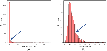
  Figure 6: Setting of dynamic threshold based on the histogram. (a) and (b) show the histogram of confidence score group and paired IoU group, respectively. The blue arrow points correspond to the steepest descent point, i.e., the selection of the dynamic threshold.

• Adaptive density curriculum setup. Different datasets are collected by different quality of LiDAR, resulting in drastic density variations in the point clouds. To enable the model to adapt to different datasets, we propose to use the following linear curriculum function to set $\lambda^{k}_{ic}$:

  $$\lambda^{k}_{ic}(t)=\max(d_{min}^{c},d_{0}^{c}-\frac{d_{0}^{c}-d_{min}^{c}}{\mathcal{T}_{\text{down}}}\cdot t),$$ (29)

  where the initial density value $d_{0}^{c}$ for class $c$ of a training scene can be written as

  $$d_{0}^{c}=\frac{1}{\sum_{i=1}^{M}N_{i}}\sum_{i=1}^{M}\sum_{j=1}^{N_{i}}d(r_{ij}^{c}(\phi^{(0)})),c=1,\cdots,C.$$ (30)

  We use $d_{0}=(d_{0}^{1},\cdots,d_{0}^{C})$ to denote initial density value vector for all classes. Here, $\phi^{(0)}$ represents the model weight of the detector trained directly on the sparsely annotated dataset $\tilde{D}$, $r_{ij}^{c}$ is the bounding box generated by the detector $F(\cdot;\phi^{(0)})$. Besides, $d_{min}^{c}$ denotes the minimum density of the hardest instances, and ${\mathcal{T}_{\text{down}}}$ denotes the preset training iteration steps (We set it as the four-fifth of the total training steps). By this formulation, different classes are separately handled by considering their inherently different densities, and we filter out the bounding box predictions whose densities are less than $\lambda^{k}_{ic}(t)$ for class $c$ at the $t$-th training round.

Algorithm 2 Algorithm of Confident Missing-Annotated Instance Mining.

0:  Teacher detector $F_{m}$ with weight parameter $\phi^{(t)}$ at round $t$, instance bank ${\mathcal{B}^{(t)}}$, sparsely annotated dataset $\tilde{\mathcal{D}}$, initial density $d_{0}$, global augmentation strategies $\mathcal{A}$;

1:  for  $P_{i}$ in $\tilde{\mathcal{D}}$  do

2:     Obtain $\hat{P}_{i}=\mathcal{A}({P}_{i})$ by applying global augmentation strategies $\mathcal{A}$ to original scene $P_{i}$;

3:     Obtain ${E}_{i}$ and $\hat{{E}}_{i}$ by inputting $P_{i}$ and $\hat{P}_{i}$ to the detector $F_{m}(\cdot;\phi^{(t)})$ based on Eq. 5;

4:     Set $\lambda^{u}_{ic},\lambda^{v}_{ic},\lambda^{v}_{ic}$ by adaptive sample selection curriculum setups in Section 4.2.2;

5:     Perform joint multi-criteria sample selection process via Eq. 18, Eq. 21 and Eq. 24;

6:     Generate high quality of pseudo annotations $\tilde{U}_{i}$ for selected instances via Eq. 25;

7:     Update instance bank $\mathcal{B}_{i}^{(t)}$ by adding newly selected confident missing-annotated instances, denoted by $\mathcal{B}_{i}^{(t+1)}$.

8:  end for

8:  Updated instance bank $\mathcal{B}_{i}^{(t+1)}$

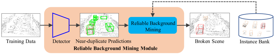
Figure 7: Illustration of the proposed reliable background mining module. To start, we feed the original point cloud to the detector without NMS to produce near-duplicate predictions, and leverage the instances stored in the instance bank to filter out unreliable 3D object points. This will lead to broken scene with reliable background, which is further processed through the GT sampling data augmentation in Section 4.4.

The illustration of the confident missing-annotated instance mining process can be found in Fig. 4, and the algorithm for this process is shown in Algorithm 2. The final selected pseudo instances are stored in the instance bank $\mathcal{B}$, with their point cloud inside the 3D bounding boxes and predicted class labels. By these sample selection curriculums, when the detector becomes more mature (i.e., in the subsequent iterations), the negative influence of missing-annotated instances gradually decreases and our instance bank can store more and more confident positive instances to further support the reliable background mining process. Noted that we do not perform pseudo instance mining in the first iteration, since many missing-annotated instances bring poor detection performance at the early training stage.

Remark. Different from traditional SPL [53, 42] modelling selection variables and model parameter in the same-level optimization problem, we formulate selection variables and model parameter as outer- and inner-level optimization, respectively, which is a typical bi-level optimization problem [40, 41]. More recently, several works attempt to learn selection variables using an unbiased meta data [44, 45, 5, 8] in a meta-learning manner. Comparatively, we regard the well-studied SPL model as meta-knowledge [1] to help promote better multi-criteria sample selection process. More importantly, we use multi-criteria sample selection curriculums to jointly mine confident missing-annotated instances, which is more effectively and robustly to filter out unreliable 3D object instances compared with previous single-criteria methods [54, 58].

Though the confident missing-annotated instances mining module mines some high-quality positive instances, there are still omissions, which naturally lead to the detector overfitting to the unreliable background (the missing-annotated instances and the region near those instances may be incorrectly marked as background). Hence, we propose a reliable background mining module to possibly mine reliable background.

4.3 Reliable Background Mining

In this section, the principles and mechanisms of step 9 in Algorithm 1 are elaborated in detail. To reduce the possibility of wrongly labeling positive instances as background, it is encouraged to mine potential foreground points as far as possible, and then the remains should be the reliable background. To this goal, we propose the reliable background mining module shown in Fig. 7. Specifically, we firstly set a low confidence score threshold for the detector. Then, to eliminate the foreground points omissions issue caused by inaccurate location boxes, frequently occurring at the initial training phase of the detector, we remove the Non-Maximum Suppression (NMS) operation [61, 62] to get near-duplicate prediction results as illustrated in Fig. 8. Those two simple strategies can guarantee that the produced results contain potential foreground points as far as possible, and the detailed recall rate analysis can be seen in Fig. 15 (a).

As illustrated in Fig. 7, we construct an instance bank which initially just stores the sparsely annotated instances and then progressively stores mined highly confident pseudo instances (please see in Section 4.2). Specifically, we denote the predicted 3D bounding boxes as $R_{i}$, and the bounding boxes of the scene $P_{i}$ in instance bank $\mathcal{B}$ as $\mathcal{B}_{i}$, which contains the sparsely annotated instance and previously mined pseudo instances. And then we delete all points of the predicted bounding boxes $R_{i}$ in the scene $P_{i}$ to get the confident scene $\tilde{P}_{i}$. Next, the bounding boxes and corresponding points stored in the instance bank $\mathcal{B}_{i}$ of the $i$-th scene will fill into the scene $P_{i}$. The instance bank helps to avoid wrongly discarding reliable 3D objects whilst removing the ambiguous points for each training scene.

The whole pipeline is illustrated in Fig. 7, and the learning process is presented in Algorithm 3. The final obtained broken scenes via Algorithm 3 contain reliable background and some confident foreground objects.

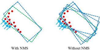
Figure 8: Illustration of detection results with NMS (left) and without NMS (right), where the green and blue dashed boxes represent the ground truth and predicted bounding box, respectively. To handle the omission of foreground points (red points pointed by blue arrows) due to inaccurate location boxes, we remove the NMS operation from the detector.

Algorithm 3 Algorithm of Reliable Background Mining.

0:  Teacher detector $F_{m}$ with weight parameter $\phi^{(t)}$ at round $t$, instance bank ${\mathcal{B}^{(t)}}$, sparsely annotated dataset $\tilde{\mathcal{D}}$, low score threshold $\tau_{low}$;

1:  Initialize empty scene set $\tilde{P}^{(t)}$;

2:  for  $P_{i}$ in $\tilde{\mathcal{D}}$  do

3:     Obtain ${E}_{i}$ via Eq. (5) by setting the detector $F_{m}$ w/o NMS operation and w/ threshold $\tau_{low}$;

4:     Fetch 3D objects ${\mathcal{B}_{i}}$ from instance bank $\mathcal{B}^{(t)}$;

5:     Delete all points of ${E}_{i}$ for the scene $P_{i}$;

6:     Generate the confident scene $\tilde{P}_{i}^{(t)}$ by filling all points of ${\mathcal{B}_{i}}$ for the scene $P_{i}$;

7:     $\tilde{P}^{(t+1)}$ = $\tilde{P}^{(t)}\cup\tilde{P}_{i}^{(t)}$;

8:  end for

8:  Broken scenes set $\tilde{P}^{(t+1)}$ with reliable background.

4.4 Confident Fully-Annotated Scene Generation

While reliable background mining eliminates most of the ambiguity in supervision, the point cloud scene may only contain a few instances of ground truth, and the distribution of these instances may differ significantly from that of real scenes. This can significantly degrade the network’s performance if they are used directly for training. Following the idea of GT-Sampling [10] data augmentation, we propose to generate confident fully-annotated scenes by combining mined positive instances from constantly updated instance bank and generating broken scenes with reliable background, which enables the the 3D detector to learn from high-quality fully-annotated scenes supervision signals under challenging sparsely-annotated setting. Now, the training process of teacher and student detector can be obtained via Eqs. (27) and (28).

TABLE I: Comparison with different detectors trained with full annotations and extremely sparse split (20% instances of full annotations) on KITTI val split, where green numbers represent decrease, red numbers represent increase. We report the mAP with 40 recall positions.

Method	Data	3D Detection (Car)			BEV Detection (Car)			3D Detection (Ped.)			BEV Detection (Ped.)			3D Detection (Cyc.)			BEV Detection (Cyc.)
		Easy	Mod	Hard	Easy	Mod	Hard	Easy	Mod	Hard	Easy	Mod	Hard	Easy	Mod	Hard	Easy	Mod	Hard
1. PointRCNN[14]	Full	89.66	80.59	78.05	93.19	89.13	86.84	61.58	54.58	47.93	66.27	58.26	51.57	89.03	70.61	66.34	91.99	71.90	69.53
2. PointRCNN[14]	Sparse (20%)	64.33	54.91	53.97	77.50	71.31	70.84	39.35	32.41	28.40	42.14	36.13	31.03	60.46	46.95	43.45	63.17	48.34	44.61
3. SS3D++ (Ours)	Sparse (20%)	91.80	79.85	77.65	95.83	88.37	86.48	63.95	55.98	48.13	67.25	59.98	51.39	89.84	74.13	70.51	92.87	77.30	72.65
4. Improved 2 $\rightarrow$ 1	-	-25.33	-25.68	-24.08	-15.69	-17.82	-16.00	-22.23	-22.17	-19.53	-24.13	-22.13	-20.54	-28.57	-23.66	-22.89	-28.82	-23.56	-24.92
5. Improved 3 $\rightarrow$ 1	-	+2.14	-0.74	-0.40	+2.64	-0.76	-0.36	+2.37	+1.40	+0.20	+0.98	+1.72	-0.18	+0.81	+3.52	+4.17	+0.88	+5.40	+3.12
1. Part-A2[15]	Full	92.15	82.91	81.99	92.90	90.06	88.35	66.88	59.67	54.62	70.53	64.19	59.24	90.34	70.13	66.92	91.95	74.63	70.63
2. Part-A2[15]	Sparse (20%)	78.54	68.81	67.03	85.05	79.63	78.03	45.73	41.37	38.40	50.32	45.95	43.17	73.61	55.10	50.76	75.09	57.77	53.26
3. SS3D++ (Ours)	Sparse (20%)	92.74	82.19	81.11	95.93	89.32	87.83	68.86	62.40	57.26	71.51	65.80	60.12	92.35	74.77	70.87	93.46	75.75	71.60
4. Improved 2 $\rightarrow$ 1	-	-13.61	-14.10	-14.96	-7.85	-10.43	-10.32	-21.15	-18.30	-16.22	-20.21	-18.24	-16.07	-16.73	-15.03	-16.16	-16.86	-16.86	-17.37
5. Improved 3 $\rightarrow$ 1	-	+0.59	-0.72	-0.88	+3.03	-0.74	-0.52	+1.98	+2.73	+2.64	+0.98	+1.61	+0.88	+2.01	+4.64	+3.95	+1.51	+1.12	+0.97
1. PV-RCNN[6]	Full	92.10	84.36	82.48	93.02	90.32	88.53	63.12	54.84	51.78	65.18	59.41	54.51	89.10	70.38	66.01	93.45	74.53	70.10
2. PV-RCNN[6]	Sparse (20%)	74.25	64.72	62.78	82.19	77.23	76.25	54.97	49.89	45.62	58.45	53.37	49.94	81.73	61.27	56.90	84.49	65.65	61.24
3. SS3D++ (Ours)	Sparse (20%)	92.54	84.40	82.28	95.91	90.59	88.43	58.94	54.44	49.66	61.76	57.55	52.89	91.61	76.21	71.46	94.62	78.18	73.62
4. Improved 2 $\rightarrow$ 1	-	-17.85	-19.64	-19.70	-10.83	-13.09	-12.28	-8.15	-4.95	-6.16	-6.73	-6.04	-4.57	-7.37	-9.11	-9.11	-8.96	-8.88	-8.86
5. Improved 3 $\rightarrow$ 1	-	+0.44	+0.04	-0.20	+2.89	+0.27	-0.10	-4.18	-0.40	-2.12	-3.42	-1.86	-1.62	+2.51	+5.83	+5.45	+1.17	+3.65	+3.52
1. Voxel-RCNN[23]	Full	92.38	85.29	82.86	95.52	91.25	88.99	-	-	-	-	-	-	-	-	-	-	-	-
2. Voxel-RCNN[23]	Sparse (20%)	75.55	64.67	62.43	83.34	76.75	73.50	-	-	-	-	-	-	-	-	-	-	-	-
3. SS3D++ (Ours)	Sparse (20%)	93.59	83.83	82.79	96.71	91.70	89.26	-	-	-	-	-	-	-	-	-	-	-	-
4. Improved 2 $\rightarrow$ 1	-	-16.83	-20.62	-20.43	-12.18	-14.50	-15.49	-	-	-	-	-	-	-	-	-	-	-	-
5. Improved 3 $\rightarrow$ 1	-	+1.21	-1.46	-0.07	+1.19	+0.45	+0.27	-	-	-	-	-	-	-	-	-	-	-	-

TABLE II: Comparison with SS3D [52] trained with extremely sparse split on KITTI val split. The 3D detection and BEV detection are evaluated by mean average precision with 11 recall positions. The IoU thresholds are 0.7 for car and 0.5 for cyclist, respectively.

Method	Data	3D Detection (Car)			BEV Detection (Car)			3D Detection (Cyc.)			BEV Detection (Cyc.)			Average
		Easy	Mod	Hard	Easy	Mod	Hard	Easy	Mod	Hard	Easy	Mod	Hard
SS3D (PointRCNN-based [14])	Sparse	87.18	77.10	76.13	89.74	87.41	85.71	86.62	73.22	66.92	87.21	74.27	71.54	80.25
SS3D++ (PointRCNN-based [14])	Sparse	88.63	77.90	77.13	90.26	87.65	86.10	86.73	74.81	70.28	87.76	74.64	71.81	81.14
SS3D (PV-RCNN-based [6])	Sparse	89.49	79.30	78.28	90.45	87.98	87.00	88.01	70.35	67.40	89.72	72.33	70.14	80.87
SS3D++ (PV-RCNN-based [6])	Sparse	89.32	83.42	78.67	90.23	87.91	87.33	88.33	76.13	70.72	93.99	77.54	72.42	82.89

5 Experiments

5.1 Datasets and Evaluation Metrics

Following the SOTA methods [56, 57], we evaluate our SS3D++ on two widely acknowledged 3D object detection datasets: KITTI [13] and Waymo Open Dataset [9].

KITTI Dataset The KITTI 3D and BEV object detection benchmark [13] are widely used for performance evaluation. There are 7,481 samples for training and 7,518 samples for testing and we further divide the training samples into a train split of 3,712 samples and a val split of 3,769 samples as a common practice [6]. In addition, due to the occlusion and truncation levels of objects, the KITTI benchmark has three difficulty levels in the evaluation: easy, moderate, and hard. As for sparsely annotated dataset generation, we randomly keep one annotated object in each 3D scene from train split to generate the extremely sparse split. Compared with the full annotation of all objects on KITTI, the extremely sparse split only needs to be annotated with 20% of objects. For fair comparisons with previous methods, we report the mAP with 40 or 11 recall positions  [24, 56], with a 3D overlap threshold of 0.7, 0.5, and 0.5 for the three classes: car, pedestrian, and cyclist, respectively. All the models are evaluated on the val split.

Waymo Open Dataset The Waymo Open Dateset is a large-scale benchmark that includes point cloud and RGB images from a LiDAR sensor and five cameras, respectively. The dataset contains 798 training sequences with around 160k point cloud samples, and 202 validation sequences with 40k point cloud samples, which are annotated in a 360-degree field. Based on an IoU threshold of 0.7 for vehicles and 0.5 for pedestrians/cyclists. The official 3D detection evaluation metrics including 3D bounding box mean average precision (mAP) and mAP weighted by heading accuracy (mAPH) are used to benchmark the performance for objects of two difficulty levels (LEVEL_1 and LEVEL_2). Following the experiments setting of PV-RCNN++[56] in OpenPCDet [22], we sample 20% of data (about 32k samples) with a frame interval of 5, which includes 1,412k annotated 3D bounding boxes. Following sparsely annotated dataset generation in the KITTI dataset, we randomly keep one annotated object in each scene to generate the extremely sparse split. Compared with the full annotation of all objects on the Waymo dataset, the extremely sparse split only needs to be annotated with about 2.2% of objects.

5.2 Implementation Details

We implement our method following OpenPCDet [22] with the extremely sparse split, and keep the default supervised loss and configurations as the used detector. At the training stage, for the KITTI and Waymo, we also adopt the default optimization setting of the original detector (e.g., ADAM optimizer and cosine annealing learning rate[31]) with the total rounds of 10 and 6, respectively. We set the low score threshold $\tau_{l}$ as 0.01 in reliable background selection. In our global augmentation, we randomly flip each scene along X-axis and Y-axis with 0.5 probability, and then scale it with a uniformly sampled factor from $[0.8,1.2]$. Finally, we rotate the point cloud around Z-axis with a random angle sampled from $\left[-\frac{\pi}{4},\frac{\pi}{4}\right]$.

TABLE III: Comparison on 202 validation sequences with different detectors trained with fully annotated and extremely sparse annotated Waymo Open Dataset. All detectors are implemented based on [22]. †: with centerhead [63].

Method	Data	Veh.(LEVEL_1)		Veh.(LEVEL_2)		Ped.(LEVEL_1)		Ped.(LEVEL_2)		Cyc.(LEVEL_1)		Cyc.(LEVEL_2)		Avg.
		mAP	mAPH	mAP	mAPH	mAP	mAPH	mAP	mAPH	mAP	mAPH	mAP	mAPH
PartA2[15]	Full	74.66	74.12	65.82	65.32	71.71	62.24	62.46	54.06	66.53	65.18	64.05	62.75	65.74
PartA2[15]	Sparse	43.95	42.40	38.35	37.00	24.27	19.51	20.37	16.36	49.92	48.46	48.02	46.61	36.27
Ours (PartA2-based)	Sparse	66.27	65.35	58.03	57.02	52.54	45.68	44.37	38.46	60.71	58.80	58.12	56.67	55.17
†Voxel-RCNN [23]	Full	76.13	75.66	68.18	67.74	78.20	71.98	69.29	63.59	70.75	69.68	68.25	67.21	70.56
†Voxel-RCNN [23]	Sparse	47.83	46.32	41.83	40.51	25.88	20.73	21.78	17.44	50.29	48.48	48.38	46.65	38.01
Ours(Voxel-RCNN-based)	Sparse	65.99	65.29	57.50	56.90	53.44	48.89	46.41	42.37	60.13	58.93	57.40	56.26	55.79
PV-RCNN++ [56]	Full	77.82	77.32	69.07	68.62	77.99	71.36	69.92	63.74	71.80	70.71	69.31	68.26	71.33
PV-RCNN++ [56]	Sparse	29.96	29.20	25.95	25.29	12.26	10.35	10.20	8.61	43.66	42.54	41.99	40.91	26.74
Ours (PV-RCNN++-based)	Sparse	65.73	64.96	57.34	56.67	53.62	48.51	45.33	41.01	59.78	58.36	57.06	55.72	55.34
CenterPoint [63]	Full	71.33	70.76	63.16	62.65	72.09	65.49	64.27	58.23	68.68	67.39	66.11	64.87	66.25
CenterPoint [63]	Sparse	32.98	32.33	28.82	28.24	20.22	16.91	17.30	14.47	28.84	27.90	27.74	26.84	25.22
Ours(CenterPoint-based)	Sparse	63.49	62.93	55.30	54.81	48.93	43.89	41.53	37.22	51.87	50.81	50.07	49.04	50.82

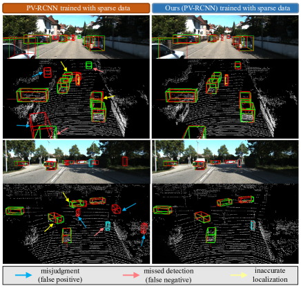
Figure 9: Qualitative comparison results of the PV-RCNN [6] and our SS3D++ method (PV-RCNN-based) trained with sparsely-annotated data. The ground truth 3D bounding boxes of cars, cyclists, and pedestrians are drawn in green, yellow, and cyan, respectively. We set the predicted bounding boxes in red and project boxes in the point cloud back onto the color images for visualization.

5.3 Comparisons with Fully-Supervised Methods

Comparison with fully-supervised methods on KITTI. To evaluate our SS3D++ framework on the highly-competitive KITTI dataset, we compare the proposed method with four SOTA fully-supervised methods: PointRCNN [14], Part-A² [15], PV-RCNN [6], Voxel-RCNN [23], with fully-annotated train split and the extremely sparse train split, respectively, where these detectors trained on the extremely sparse split are used as the initial detectors of our method. The results of different methods are shown in Table I. From this table, it can be seen that the four fully-supervised detectors trained on the sparsely annotated dataset produce a significant performance degradation due to the extremely inexact and incomplete supervision. For example, PointRCNN has an average performance decrease of approximately 25% points on “car” 3D detection, 21% points on “pedestrian” 3D detection, and 25% points on “cyclist” 3D detection. Even for the competitive PV-RCNN detector, it exhibits an average decline of about 19% points on “car” 3D detection, 6% points on “pedestrian” 3D detection, and 8% points on “cyclist” 3D detection. In the left column of Fig. 9, we visualize the detection results of PV-RCNN on the KITTI dataset. As shown, there exist some typical mistakes for the PV-RCNN detector, e.g., the background wrongly detected as an object (indicated by blue arrows), missing object detection (pink arrows), inaccurate localization (yellow arrows), etc.

Our SS3D++ method is detector-agnostic and can be easily used to further improve these off-the-shelf 3D fully-supervised detectors with sparse supervision. Table I shows that our SS3D++ method can substantially boost the detection performance of different fully-supervised detectors for each category across different difficulty levels, and approaches or even surpasses the results of these methods with full supervision. This highlights the significant advantage of the proposed method in eliminating the negative influence of sparse supervision. The visual qualitative analysis of detection results is shown in the right column of Fig. 9. As can be seen, the SS3D++ method effectively overcomes the mistakes of the PV-RCNN detector, and achieves fine detection results. The visualization results of other detectors can be found in Appendix Fig. 1. This further validates the effectiveness of iterations between detector amelioration and confident fully-annotated scene generation.

Table II further compares the SS3D++ method with our previous conference method SS3D. The novel SS3D++ method outperforms the previous SS3D method by a margin on three different difficulty levels for all categories. These consistent improvements demonstrate the effectiveness of the mutual benefit of our SS3D++ between 3D detector training and confident fully-annotated scene generation.

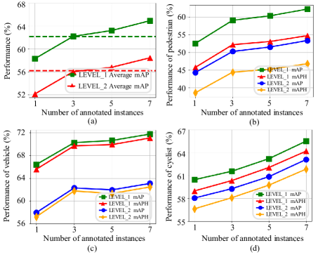
Figure 10: Detection performance against the number of annotated instances per scene on the Waymo dataset.

Comparison with fully-supervised methods on Waymo. The Waymo dataset is larger than the KITTI dataset and the scene is very crowded, with an average of 44 objects in each scene. Thus it is relatively difficult and expensive to provide full precise annotations. The proposed framework of using extremely sparse annotation can effectively reduce the workload to a greater extent (about 2.2% points). However, such sparse annotation significantly deteriorates the existing fully-supervised detectors. As shown in Table III, PartA² and Voxel-RCNN have an average performance decrease of beyond 29% and 32% points, respectively. To further verify the generalizability of our SS3D++, we also replace the base detector with two latest networks that are different from those in the KITTI experiment, i.e., PV-RCNN++[56] and CenterPoint [63]. While they encounter an average performance decrease of beyond 44% and 41% points, respectively.

Nonetheless, our SS3D++ method can still achieve about 80% performance compared with the detectors trained with full supervision and improves the average detection performance of PartA², Voxel-RCNN, PV-RCNN++, and CenterPoint by 18.90%, 17.76%, 28.60%, 25.60% points, respectively. This demonstrates that SS3D++ method can achieve a consistent performance improvement across different datasets/detectors. Observing that we only have access to only 2.2% precise annotations, this implies that the SS3D++ method is hopeful to be readily applied to real-world 3D object detection that requires low-cost annotations. The qualitative comparison results on the Waymo Open dataset can be found in Appendix Fig. 2.

Due to the crowded nature of the Waymo dataset, the distribution of objects within the scenes is usually dense. When we only annotate one instance per scene, it poses significant challenges for detection learning. The large number of missing annotated instances results in seriously incomplete supervision, which causes a detrimental performance. We further attempt to annotate more instances for each scene to improve the performance. Fig. 10 illustrates the varying curve of average detection performance as the number of annotated instances increase per scene. It can be observed that we could achieve about 90% of the performance achieved by fully supervised methods (as depicted by the dashed line in Fig. 10 (a)) with only additionally annotating two objects per scene. Especially, we only require about $15\times$ less annotation cost compared with full annotation. We also show the varying curve of detection performance in terms of the vehicle, pedestrian, and cyclist categories in Fig. 10 (b, c, d). It can be seen that the detection performance of different categories can be progressively improved as the number of annotated instances increase per scene. This implies that the SS3D++ method is capable of boosting performance by employing more annotation information.

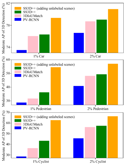
Figure 11: Performance comparison on KITTI val split with semi-supervised 3DIoUMatch [11] method trained with 1% or 2% labeled data. Both SS3D++ and 3DIoUMatch methods are based on PV-RCNN [6]. We report the mAP with 40 recall positions for a fair comparison.

TABLE IV: Performance comparison on KITTI val split with center-click weakly-supervised WS3D [24] method. We report the mAP with 11 recall positions. ‘*’ denotes the scenes with center-click annotations and ‘${\dagger}$’ denotes precisely-annotated instances.

Training Data	Method	3D Detection (Car)			BEV Detection (Car)			Avg.
		Easy	Mod	Hard	Easy	Mod	Hard
500* scenes + 534† instances	WS3D [24]	85.04	75.94	74.38	88.95	85.83	85.03	82.52
534† instances	Ours (PointRCNN-based [14])	84.69	71.93	67.06	89.57	84.07	78.81	79.36
	Ours (PartA2-based [15])	88.56	77.91	72.46	90.00	86.45	82.28	82.94
	Ours (Voxel-RCNN-based [23])	88.37	77.72	75.07	90.19	87.33	84.28	83.83
	Ours (PV-RCNN-based [6])	89.26	78.8	76.55	90.19	87.24	85.05	84.52

5.4 Comparisons with Weakly-Supervised Methods

Comparison with the semi-supervised method. We compare the proposed SS3D+ method with semi-supervised method 3DIoUMatch [11], which is based on the advanced detector PV-RCNN [6]. To make a fair comparison, we also adopt the PV-RCNN as the base detector and keep all methods trained with the same number of annotated objects. Specifically, in the KITTI train split, there are 3,712 scenes and these scenes contain a total of 17,289 objects for cars, pedestrians, and cyclists. For semi-supervised methods, 1% labeled data means 37 ($3712\times 1\%$) scenes, which include an average of 172 ($17289\times 1\%$) labeled objects used for training. So as for 1% labeled data in our extremely sparse split, we randomly select 172 scenes including 172 labeled objects for training. We also test the case of 2% labeled training data for both methods. Generally, our sparse annotation strategy may provide an easier way to annotate objects from point cloud scenes compared to a dense annotation strategy for semi-supervised methods. The detection results with different ratios of labeled data can be seen in Fig. 11. As we can see, our SS3D++ (the green bar) significantly outperforms the current SOTA semi-supervised method, 3DIoUMatch, for three different classes with all ratios of labeled training data split. Fig. 12 illustrates the comparison of mining pseudo instances by 3DIoUMatch and SS3D++ methods. The 3DIoUMatch method may easily fall into a suboptimal solution due to limited information transfer from labeled to large discrepancy unlabeled scenes, while the SS3D++ method can encourage easier intra-scene information transfer due to the proposed sparse annotation strategy, in which each scene has one object annotation. In fact, the results of the green bar in Fig. 11 only use 172 (or 344) scenes for training, while 3DIoUMatch has access to all 3712 scenes involved in training. This illustrates the potential of the SS3D++, and we can further boost the performance of the SS3D++ by utilizing the remaining unlabeled scenes, and obtain more improvements as depicted by the yellow bar in Fig. 11, outperforming 3DIoUMatch method by a large margin (more details can refer to Section 5.6).

Comparison with the center-click weakly-supervised method. For the weakly-supervised method, WS3D [24], trains the detector with the first 500 scenes with center-click labels, mixed with randomly selected 534 precisely-annotated instances. Since the standard detectors are not applicable with center-click labels, we only use the same number of (534) precisely-annotated instances randomly chosen from the first 534 scenes to train our proposed SS3D++ method. From Table IV, we can easily observe that the SS3D++ method is able to achieve better performance than WS3D for three different base detectors. WS3D may suffer from the significant disparity between point-level weak annotations and 3D precise annotations, which we only have access to precisely-annotated instances, without point-level annotation efforts, which prevents detectors from overfitting the disparity. Moreover, it is worth noting that we can obtain better performance gains when we use more powerful detectors, e.g., from PointRCNN to PartA². This highlights the advantage of our detector-agnostic framework, hinting at the potential of our method which employs advanced SOTA detectors to achieve competitive performance. Besides, the SS3D++ method can employ additional unlabeled scenes to further boost the performance (refer to Section 5.6), while WS3D cannot. This makes our SS3D++ easily apply to real-world 3D detection.

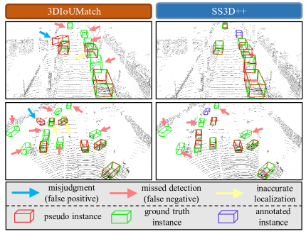
Figure 12: Qualitative comparison of mining pseudo instances by 3DIoUMatch [11] and SS3D++ methods.

5.5 Ablation Study and Analysis

In this section, we present a series of ablation studies to analyze the effects of different modules in our proposed SS3D++ method. Following the aforementioned setting, all models are trained on the KITTI dataset with an extremely sparse split and evaluated on the val split. We take PointRCNN[14] as an example base detector to conduct our ablation study, and our methods can obtain similar results for other detectors. Table V summarizes the ablation results on our reliable background mining module (RBMM) and confident missing-annotated instances mining module (CMIM). All results are reported by the mAP with 40 recall positions under moderate difficulty.

Effect of the reliable background mining module. In the $1^{st}$ row of Table V, we discarded both modules, so it represents the standard PointRCNN detector trained with the extremely sparse split, whose performances have significant degradation compared with full annotations. In the $2^{nd}$ row, we leverage the reliable background mining module to extract reliable backgrounds. It can be observed that the performance of the three categories is significantly improved, especially for the ”car” category, which has shown a substantial increase. This is due to that the autonomous driving dataset usually contains the largest number of cars. Therefore, under the sparsely-supervised setting, the detector trained with massive missing-annotated instances like cars may severely degenerate detection performance. Fortunately, the proposed reliable background mining module could reduce the risk of treating the missing-annotated instances as background, and thereby facilitate the robust training of the detector by eliminating the negative influence of noise background in the point cloud scenes.

Furthermore, we analyze different operations of the reliable background mining module via the recall rate of removing noisy foreground points, which indicates how many point clouds belonging to missing-annotated instances in the scene are identified and then removed. The results, as illustrated in Fig. 15 (a), reveal that the joint operations of utilizing a ”low threshold“ and ”No NMS“ bring a substantial improvement in terms of recall rate. In the end, it achieves a 98% elimination of noisy foreground points and thus reduces the negative impact on the detector caused by massive missing-annotated instances.

TABLE V: Ablation study of different components for our proposed SS3D++ method. We report the mAP with 40 recall positions. RBMM: reliable background mining module. CMIM: confident missing-annotated instances mining module.

RBMM	CMIM	3D Detection (Mod.)			Avg.
		Car	Ped.	Cyc.
-	-	54.91	32.41	46.95	44.76
✓	-	79.35	47.26	66.67	64.43
-	✓	69.25	49.29	67.04	61.86
✓	✓	79.85	55.98	74.13	69.99

TABLE VI: Ablation study of different components for CMIM of our proposed SS3D++ method. We report the mAP with 40 recall positions. DLF: dynamic loss-based filtering. DCS: dynamic consistency-guided suppression. DCF: density-aware curriculum filtering.

DLF	DCS	DCF	3D Detection (Mod.)			Avg.
			Car	Ped.	Cyc.
-	-	-	79.35	47.26	66.67	64.43
✓	-	-	79.00	44.74	67.91	63.88
-	✓	-	79.62	39.90	64.10	61.21
✓	✓	-	78.94	49.49	71.36	66.66
✓	✓	✓	79.85	55.98	74.13	69.99

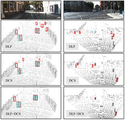
Figure 13: Qualitative comparison of mining pseudo instances for different components in the CMIM module. For ease of viewing, we only show the key instances that need to be analyzed. The ground truth 3D bounding boxes and pseudo instances of ”pedestrian” are shown in cyan and red, respectively. The combination of DLF and DCS can effectively filter out the most of erroneous pseudo instances.

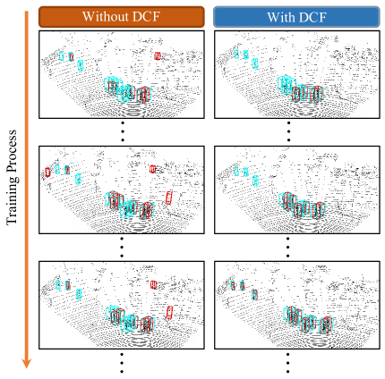
Figure 14: Visualization of pseudo instance mining with and without the DCF module. The visualization settings are similar to Fig. 13. The design of the DCF enables the discovery of more pseudo instances and significantly reduces the occurrence of false positives.

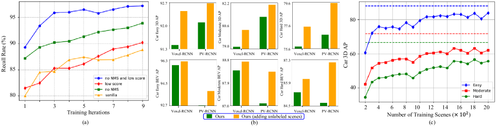
Figure 15: (a): Analysis of removal recall rate for missing-annotated foreground points with different RBMM settings. (b) Whether to add unlabeled data for performance (R40) comparison when conducting experiments with 534 sparsely annotated scenes. (c) Changing tendencies in terms of AP for SS3D++ with streaming unlabeled scenes (The dash lines represent the results learned from all unlabeled scenes in an offline manner).

Effect of the confident missing-annotated instance mining module. As shown in the $3^{rd}$ row of Table V, the confident missing-annotated instance mining module can also improve the baseline by mining high-quality instances. We can observe that the performance of the three categories is significantly improved, especially for the “pedestrian” and “cyclist” categories, which have shown better improvement compared with only RBMM. Actually, both of “pedestrian” and “cyclist” categories are relatively hard to detect compared with the ”car” category, naturally leading to more noisy pseudo-annotated instances. Our multi-criteria sample selection process can effectively filter out noisy pseudo-annotated instances, and thereby brings more robust detection performance. Therefore, it could bring mutual amelioration when we combine CMIM and RBMM ($4^{th}$ row), and achieves better performances than using either of the two.

To comprehend the roles of different components in CMIM, we further conduct a series of ablation experiments, as shown in Table VI. From the 2^nd and 3^rd row of Table VI, we can see that DLF or DCS severely deteriorates the performance of the “pedestrian” category. This is because “pedestrian” category tends to be smallest object in the training scenes, implying that the pseudo annotations are extremely noisy (even under the full supervision, the mAP score is about 60%). Both DLF and DCS depend on the quality of pseudo annotations, and thus their performance may degenerate for the “pedestrian” category with noisy pseudo annotations. While we combine DLF and DCS strategy (the 4^th row of Table VI), the mAP of the “pedestrian” category reaches +2.23% point compared with the baseline (1^st row). As shown in Fig. 13, using DLF or DCS alone leads to a significant number of erroneous pseudo instances for ”pedestrian”. However, combining both components can greatly mitigate this issue.

A large performance gain for “pedestrian” (+6% point) can be obtained when we additionally employ the DCF strategy (from the 4^th row to the 5^th row of Table VI). Meanwhile, Fig. 14 shows the quality improvement of pseudo instances by embedding the DCF with the easy-to-hard curriculum manner.

5.6 Learning from Unlabeled Training Scenes

We have studied the situation where every training scenes have sparse annotations above. Here, we consider a more practical setting, i.e., we only have access to a small number of training scenes with sparse annotations, and a large pool of unlabeled training scenes. We study two different scenarios exploiting unlabeled training scenes in the following.

Learning from unlabeled training scenes in an offline manner. In Section 5.4, our SS3D++ method only employs the sparse annotated scenes. Here, we explore to additionally exploit the remaining unlabeled scenes to train the detector. Observing from the yellow bar in Fig. 11 and Fig. 15 (b), we can see that our SS3D++ method can achieve a large improvement by utilizing additional unlabeled scenes, making it superior over weakly-supervised 3DIoUMatch [11] and WS3D [24] methods. Specifically, comparing our method with the 3DIoUMatch [11] in terms of the coverage of generated pseudo instances for unlabeled scenes, we find that 3DIoUMatch achieves only 28% coverage, while our method achieves about 60% coverage. The corresponding accuracy of mined instances in terms of the car, pedestrian, and cyclist can reach 92%, 85%, and 88% for the SS3D++ method. This highlights the potential practical value of exploiting unlabeled scenes. Additional analysis of generating pseudo-annotated instances can be found in Appendix Fig. 3 and Fig. 4. Compared with WS3D [24], our sparse supervision is easy to annotate and universal, making our method capable of generating confident pseudo annotations for easily obtained unlabeled point cloud scenes.

Learning from unlabeled training scenes in an online manner. For an autonomous driving system, it is necessary for the intelligent agent to continually acquire training data and accumulate knowledge, so as to effectively adapt to dynamic environments and driving conditions. Here, we focus on a simple preliminary attempt that incrementally learns the detector from streaming unlabeled data. Specifically, we simulate this scenario by considering a system with a memory constraint of 100 point cloud scenes. The initial model is firstly trained on 200 sparsely annotated scenes and subsequently received training scenes in an online manner. We set the online batch size to 100. Our SS3D++ method can generate reliable pseudo-annotated instances for the sequential unlabeled training scenes. After updating the detector, we randomly select the generated full-annotated scenes to update the memory, and remove the remaining training scenes. The detailed algorithm description is summarized in Appendix Algorithm 1.

Fig. 15 (c) shows the changing tendencies of mAP in sequentially involved unlabeled training scenes. As can be seen, our method can continually improve the detection performance even when we can only have access to streaming unlabeled scenes with limited memory. This result implies that our method is potentially useful for the autonomous driving system, which is required to perceive the changing environment and incrementally improve itself.

TABLE VII: Annotation analysis of three different sparsely-annotated forms.

Method	Data	Car - 3D Detection			Car - BEV Detection
		Easy	Mod	Hard	Easy	Mod	Hard
Voxel-RCNN[23]	Full	92.38	85.29	82.86	95.52	91.25	88.99
Voxel-RCNN[23]	(1) Sparse	72.97	63.05	60.23	81.64	74.91	71.93
Ours	(1) Sparse	93.50	84.36	82.64	96.63	91.31	89.02
Voxel-RCNN[23]	(2) Sparse	88.86	63.04	47.90	93.61	70.82	52.77
Ours	(2) Sparse	92.89	83.46	79.81	96.40	91.63	86.73
Voxel-RCNN[23]	(3) Sparse	29.15	42.92	49.62	35.81	53.83	60.90
Ours	(3) Sparse	94.24	84.11	82.44	96.65	91.38	88.99

5.7 Annotation Analysis

In our sparsely-annotated framework, we just annotate one 3D object per scene. One natural question is to choose which object to annotate. In practice, most annotators may be more inclined to choose the easiest object to annotate, e.g., no occluded objects or high-density objects. To further evaluate the robustness of our SS3D++ method against the hardness of annotated objects, we design the following three different annotated strategies: (1) randomly choose one object from the scene to annotate as default; (2) prioritize choosing one ‘easy’ (close and no truncated) object from the scene; (3) prioritize choosing one ‘hard’ (remote and truncated) object from the scene. Besides, we repeat the experiment 3 times and average the results to eliminate the influence of experimental randomness. From Table VII, we can observe that the hardness of annotated objects has a significant impact on the performance of the fully supervised detector, in which annotated strategy (3) severely deteriorates the detectors. However, by employing the proposed SS3D++ method, regardless of different annotated strategies, such annotation bias can be almost eliminated. Especially, the SS3D++ can achieve on-par performance compared to detectors trained with fully-supervised data for all cases. This shows our method could perform robustly with different annotated strategies, which highlights the capability of our method to effectively address such low-quality annotations. This further substantiates the potential practical value.

6 Conclusion

In this work, we study a novel weakly-annotated framework for 3D object detection from point cloud. Compared with existing densely-annotated information, we only need to annotate one object per scene. This sparse annotation strategy provides an opportunity to substantially reduce the heavy data annotation burden. We design a SS3D++ method that alternately generates high-quality fully-annotated scenes and updates the 3D detector, thereby achieving progressive amelioration of the detection model. We present extensive comparative evaluations of the SS3D++ method on the classic KITTI and more challenging Waymo Open benchmarks, and prove its capability of achieving promising performance with significantly reducing annotation cost. An important characteristic of the proposed method is detector-agnostic, which implies that it can easily benefit from advanced fully-supervised 3D detectors. Besides, the SS3D++ method is able to utilize additional unlabeled training scenes to ameliorate the model. The above results show our framework is potentially useful to help make it practical and low-budget for 3D object detection.

Though impressive results are obtained, there is still large room for further improvement. For example, it is challenging to generate high-quality pseudo-annotated instances for training scenes with crowded objects in our sparsely-supervised framework. Also, designing an effective approach to better make use of massive unlabeled training scenes is an important step towards practice. Especially, given a large number of algorithmic breakthroughs over the past few years, like meta-learning [2], foundation models [3, 4], etc, we would expect a flurry of innovation towards this promising direction.

Supplementary Material for
”Are Dense Labels Always Necessary for
3D Object Detection from Point Cloud?”

Chenqiang Gao, Chuandong Liu, Jun Shu, Fangcen Liu, Jiang Liu, Luyu Yang, Xinbo Gao, and Deyu Meng

C. Gao is with the School of Intelligent Systems Engineering, the Shenzhen Campus of Sun Yatsen University, Sun Yat-sen University, Shenzhen, Guangdong 518107, China. E-mail: gaochq6@sysu.edu.cn. C. Liu is with the School of Computer Science, Wuhan University, Wuhan 430072, China. E-mail: chuandong.liu@whu.edu.cn. J. Shu and D. Meng are with School of Mathematics and Statistics and Ministry of Education Key Lab of Intelligent Networks and Network Security, Xi’an Jiaotong University, Shaanxi 710049, China. E-mail: xjtushujun@gmail.com, dymeng@mail.xjtu.edu.cn. F. Liu and X. Gao are with School of Communication and Information Engineering, Chongqing University of Posts and Telecommunications, Chongqing 400065, China. E-mail: gaoxb@cqupt.edu.cn, liufc67@gmail.com. J. Liu is with Meta, Menlo Park 94025, USA. E-mail: jiangliu@meta.com. L. Yang is with University of Maryland, College Park 20742, USA. E-mail: loyo@umiacs.umd.edu. Manuscript received April 19, 2005; revised August 26, 2015.

Appendix A Additional Analysis of Visualization Comparison

A.1 Comparison on the KITTI Dataset

The detection results of PointRCNN [14] and PartA² [15] are shown above the dashed line in Fig. 16. As can be seen, the proposed SS3D++ method can obviously improve the detection performance and overcome the various error cases with different detector, which further demonstrates the superiority of the detector-agnostic property.

A.2 Comparison on the Waymo Open Dataset

To further verify the efficiency of our SS3D++ on the large-scale 3D autonomous driving dataset, we qualitatively show the visualization achieved by different approaches below the dashed line in Fig. 16 on the validation set of the Waymo dataset. Clearly, the SS3D++ method can effectively detect more foreground objects and prevent the missed detection, especially for the objects with small sizes (e.g., pedestrian), as well as objects far away from the LiDAR sensors. Moreover, from the analysis of the two different scenarios in the KITTI and Waymo datasets, it can be observed that directly training the original detector on sparsely annotated dataset leads to significant variations in detection errors. For example, the most common error in the KITTI dataset is false positive detection (i.e., detecting the background as foreground shown in Fig. 16), while in the Waymo dataset, the most common error is missed detection. However, our SS3D++ method greatly reduces the occurrence of these errors, further demonstrating the generalization capability of our approach. The visualization of other detectors on the Waymo can be find in Fig. 17.

Appendix B Additional Analysis of Pseudo Instances

To intuitively explore the influence of pseudo instances, we provide qualitative results of failure pseudo instance cases during the training process on 2% KITTI dataset, and the results are illustrated in Fig. 18. For ease of viewing, we only show the key instances that need to be analyzed. As we can seen, the pseudo instances of car categories is usually accurate, and common errors occur in categories that are relatively similar, such as trucks and vans (see the top box in Fig. 18). Besides, due to the small spatial size of pedestrians, it is difficult to extract corresponding features, so the common error case is low IoU caused by inaccurate localization (the middle box in Fig. 18). A similar situation occurs for cyclists. Additionally, as the bottom box shown in Fig. 18, traffic signs and poles with similar point cloud features are mistaken for pedestrians. In our future work, addressing these errors will be the focus of our research. More interestingly, our pseudo instances can also identify some instances that were manually omitted in the original dataset, as shown in Fig. 19. This situation of missed annotations typically occurs due to overcrowding of objects (such as occlusion or truncation) or insufficient lighting conditions, which may lead to the objects being overlooked by the annotator. Hence, this discovery highlights the tremendous potential of our method as an annotation tool to enhance the quality of annotations.

Appendix C Additional Analysis of Learning from Unlabeled Training Scenes in An Online Manner

For an autonomous driving system in practice, the 3D detection needs to perceive the changing environment with non-stationary data distribution and incrementally improve itself. Algorithm 4 summarizes that SS3D++ method learns from unlabeled training scenes in an online manner. In our implementation, we take Voxel-RCNN [23] as our base detector and initialize the SS3D++ method with 200 sparsely annotated sequential point cloud scenes.

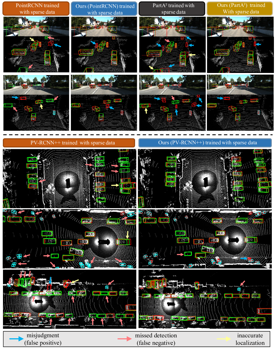
Figure 16: The qualitative comparison results on the KITTI dataset of the PointRCNN [14]/PartA² [15] and our SS3D++ method trained with sparsely-annotated data are shown above the dashed line, while the qualitative comparison results on the Waymo dataset of the PV-RCNN++ [56] and our SS3D++ method trained with sparsely-annotated data are shown below the dashed line. The ground truth 3D bounding boxes of cars, cyclists, and pedestrians are drawn in green, yellow, and cyan, respectively. For the KITTI, we set the predicted bounding boxes in red and project boxes in point cloud back onto the color images for visualization.

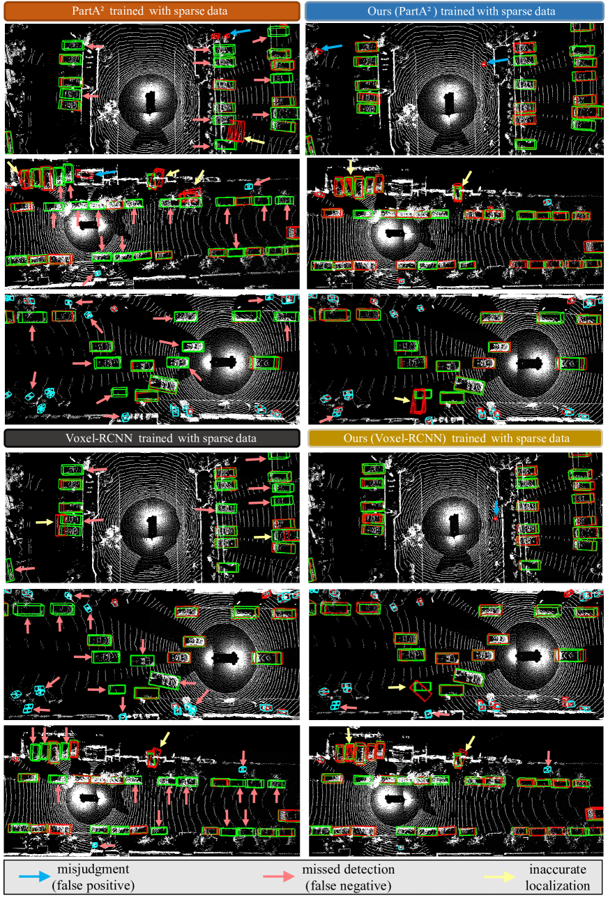
Figure 17: Qualitative comparison results of the original PartA² [15]/Voxel-RCNN [23] and our SS3D++ method trained with sparsely-annotated data on the Waymo Open dataset. The ground truth 3D bounding boxes of car and pedestrian are drawn in green and cyan, respectively. And we set the predicted bounding boxes in red.

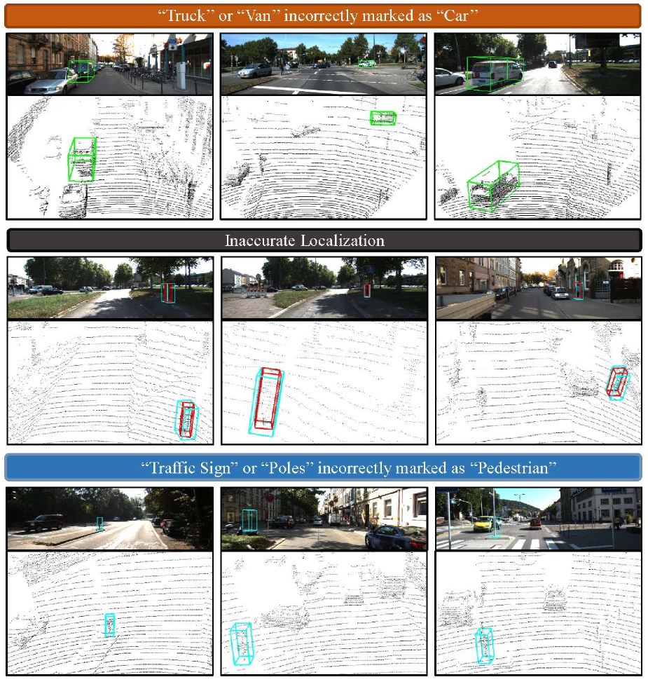
Figure 18: Visualization of failure cases of pseudo instances during the SS3D++ training process on 2% labeled data. Pseudo instance of car and pedestrian are drawn in green and red, respectively. The ground truth of pedestrian is drawn in cyan.

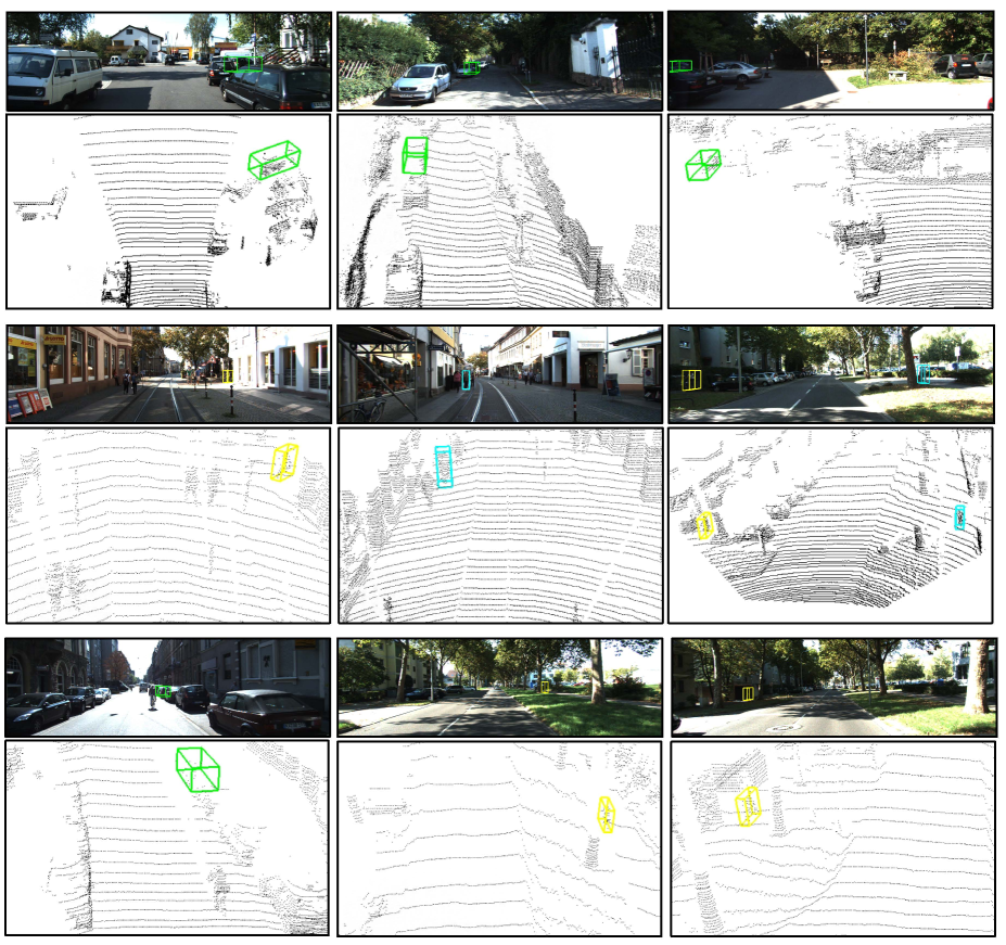
Figure 19: Visualization of interesting cases of pseudo instances during the SS3D++ training process on 2% labeled data. The pseudo instance 3D bounding boxes of car, cyclist, and pedestrian are drawn in green, yellow, and cyan, respectively.

Algorithm 4 Algorithm of Learning from Streaming Unlabeled Scenes.

0:  $\mathcal{S}_{t}$: stream unlabeled scenes at time $t$, $\mathcal{M}$: scenes stored in memory, $T$: the number of streaming tasks, 3D detector $F$ with weight parameter $\phi$.

1:  Initialize 3D detector $F$ using the SS3D++ method with initial sparsely annotated scenes and update weight parameter $\phi$;

2:  for  $t=1$ to $T$  do

3:     Fetch current streaming unlabeled scenes $\mathcal{S}_{t}$ and memory scenes $\mathcal{M}$;

4:     Alternatively improve 3D detector training and confident fully-annotated scene generation using the SS3D++ method based on $\mathcal{S}_{t}\cup\mathcal{M}$.

5:     Update memory $\mathcal{M}$ by randomly selecting generated full-annotated scenes, and remove the remaining training scenes.

6:  end for

6:  Learned 3D detector $F$

References

- [1] J. Shu, X. Yuan, D. Meng, and Z. Xu, “Dac-mr: Data augmentation consistency based meta-regularization for meta-learning,” arXiv preprint arXiv:2305.07892, 2023.
- [2] J. Shu, D. Meng, and Z. Xu, “Learning an explicit hyperparameter prediction function conditioned on tasks,” Journal of Machine Learning Research, 2023.
- [3] R. Bommasani, D. A. Hudson, E. Adeli, R. Altman, S. Arora, S. von Arx, M. S. Bernstein, J. Bohg, A. Bosselut, E. Brunskill et al., “On the opportunities and risks of foundation models,” arXiv preprint arXiv:2108.07258, 2021.
- [4] A. Kirillov, E. Mintun, N. Ravi, H. Mao, C. Rolland, L. Gustafson, T. Xiao, S. Whitehead, A. C. Berg, W.-Y. Lo et al., “Segment anything,” arXiv preprint arXiv:2304.02643, 2023.
- [5] J. Shu, X. Yuan, and D. Meng, “Cmw-net: an adaptive robust algorithm for sample selection and label correction,” National Science Review, vol. 10, no. 6, p. nwad084, 2023.
- [6] S. Shi, C. Guo, L. Jiang, Z. Wang, J. Shi, X. Wang, and H. Li, “Pv-rcnn: Point-voxel feature set abstraction for 3d object detection,” in CVPR, 2020, pp. 10 529–10 538.
- [7] T.-Y. Lin, P. Goyal, R. Girshick, K. He, and P. Dollár, “Focal loss for dense object detection,” in ICCV, 2017, pp. 2980–2988.
- [8] J. Shu, D. Meng, and Z. Xu, “Meta self-paced learning,” Scientia Sinica Informationis, vol. 50, no. 6, pp. 781–793, 2020.
- [9] P. Sun, H. Kretzschmar, X. Dotiwalla, A. Chouard, V. Patnaik, P. Tsui, J. Guo, Y. Zhou, Y. Chai, B. Caine et al., “Scalability in perception for autonomous driving: Waymo open dataset,” in CVPR, 2020, pp. 2446–2454.
- [10] Y. Yan, Y. Mao, and B. Li, “Second: Sparsely embedded convolutional detection,” Sensors, vol. 18, no. 10, p. 3337, 2018.
- [11] H. Wang, Y. Cong, O. Litany, Y. Gao, and L. J. Guibas, “3dioumatch: Leveraging iou prediction for semi-supervised 3d object detection,” in CVPR, 2021, pp. 14 615–14 624.
- [12] W. Zheng, W. Tang, L. Jiang, and C.-W. Fu, “Se-ssd: Self-ensembling single-stage object detector from point cloud,” in CVPR, 2021, pp. 14 494–14 503.
- [13] A. Geiger, P. Lenz, C. Stiller, and R. Urtasun, “Vision meets robotics: The kitti dataset,” Int. J. Rob. Res., vol. 32, no. 11, pp. 1231–1237, 2013.
- [14] S. Shi, X. Wang, and H. Li, “Pointrcnn: 3d object proposal generation and detection from point cloud,” in CVPR, 2019, pp. 770–779.
- [15] S. Shi, Z. Wang, J. Shi, X. Wang, and H. Li, “From points to parts: 3d object detection from point cloud with part-aware and part-aggregation network,” IEEE TPAMI, vol. 43, no. 8, pp. 2647–2664, 2021.
- [16] J. Mao, S. Shi, X. Wang, and H. Li, “3d object detection for autonomous driving: A review and new outlooks,” arXiv:2206.09474, 2022.
- [17] T. Wang, T. Yang, J. Cao, and X. Zhang, “Co-mining: Self-supervised learning for sparsely annotated object detection,” in AAAI, vol. 35, no. 4, 2021, pp. 2800–2808.
- [18] H. Zhang, F. Chen, Z. Shen, Q. Hao, C. Zhu, and M. Savvides, “Solving missing-annotation object detection with background recalibration loss,” in ICASSP, 2020, pp. 1888–1892.
- [19] Y. Niitani, T. Akiba, T. Kerola, T. Ogawa, S. Sano, and S. Suzuki, “Sampling techniques for large-scale object detection from sparsely annotated objects,” in CVPR, 2019, pp. 6510–6518.
- [20] C. R. Qi, O. Litany, K. He, and L. J. Guibas, “Deep hough voting for 3d object detection in point clouds,” in ICCV, 2019, pp. 9277–9286.
- [21] Z. Wu, N. Bodla, B. Singh, M. Najibi, R. Chellappa, and L. S. Davis, “Soft sampling for robust object detection,” in BMVC, 2019, p. 225.
- [22] O. D. Team, “Openpcdet: An open-source toolbox for 3d object detection from point clouds,” https://github.com/open-mmlab/OpenPCDet, 2020.
- [23] J. Deng, S. Shi, P. Li, W. Zhou, Y. Zhang, and H. Li, “Voxel r-cnn: Towards high performance voxel-based 3d object detection,” in AAAI, vol. 35, no. 2, 2021, pp. 1201–1209.
- [24] Q. Meng, W. Wang, T. Zhou, J. Shen, Y. Jia, and L. Van Gool, “Towards a weakly supervised framework for 3d point cloud object detection and annotation,” IEEE Transactions on Pattern Analysis and Machine Intelligence, vol. 44, no. 8, pp. 4454–4468, 2021.
- [25] Z. Yang, Y. Sun, S. Liu, and J. Jia, “3dssd: Point-based 3d single stage object detector,” in CVPR, 2020, pp. 11 040–11 048.
- [26] N. Zhao, T.-S. Chua, and G. H. Lee, “Sess: Self-ensembling semi-supervised 3d object detection,” in CVPR, 2020, pp. 11 079–11 087.
- [27] A. H. Lang, S. Vora, H. Caesar, L. Zhou, J. Yang, and O. Beijbom, “Pointpillars: Fast encoders for object detection from point clouds,” in CVPR, 2019, pp. 12 697–12 705.
- [28] W. Zheng, W. Tang, S. Chen, L. Jiang, and C.-W. Fu, “Cia-ssd: Confident iou-aware single-stage object detector from point cloud,” in AAAI, vol. 35, no. 4, 2021, pp. 3555–3562.
- [29] Z. Yang, Y. Sun, S. Liu, X. Shen, and J. Jia, “Std: Sparse-to-dense 3d object detector for point cloud,” in ICCV, 2019, pp. 1951–1960.
- [30] Y. Zhang, D. Huang, and Y. Wang, “Pc-rgnn: Point cloud completion and graph neural network for 3d object detection,” in AAAI, vol. 35, no. 4, 2021, pp. 3430–3437.
- [31] I. Loshchilov and F. Hutter, “SGDR: stochastic gradient descent with warm restarts,” in ICLR, 2017.
- [32] W. Shi and R. Rajkumar, “Point-gnn: Graph neural network for 3d object detection in a point cloud,” in CVPR, 2020, pp. 1711–1719.
- [33] C. He, H. Zeng, J. Huang, X.-S. Hua, and L. Zhang, “Structure aware single-stage 3d object detection from point cloud,” in CVPR, 2020, pp. 11 873–11 882.
- [34] C. R. Qi, H. Su, K. Mo, and L. J. Guibas, “Pointnet: Deep learning on point sets for 3d classification and segmentation,” in CVPR, 2017, pp. 652–660.
- [35] K. Sohn, D. Berthelot, N. Carlini, Z. Zhang, H. Zhang, C. Raffel, E. D. Cubuk, A. Kurakin, and C. Li, “Fixmatch: Simplifying semi-supervised learning with consistency and confidence,” in NeurIPS, 2020.
- [36] C. R. Qi, L. Yi, H. Su, and L. J. Guibas, “Pointnet++: Deep hierarchical feature learning on point sets in a metric space,” in NeurIPS, 2017, pp. 5099–5108.
- [37] Y. Bengio, J. Louradour, R. Collobert, and J. Weston, “Curriculum learning,” in ICML, 2009, pp. 41–48.
- [38] M. Shi and V. Ferrari, “Weakly supervised object localization using size estimates,” in ECCV, 2016, pp. 105–121.
- [39] J. Wang, X. Wang, and W. Liu, “Weakly-and semi-supervised faster r-cnn with curriculum learning,” in ICPR, 2018, pp. 2416–2421.
- [40] R. Liu, J. Gao, J. Zhang, D. Meng, and Z. Lin, “Investigating bi-level optimization for learning and vision from a unified perspective: A survey and beyond,” IEEE Transactions on Pattern Analysis and Machine Intelligence, 2021.
- [41] L. Franceschi, P. Frasconi, S. Salzo, R. Grazzi, and M. Pontil, “Bilevel programming for hyperparameter optimization and meta-learning,” in International Conference on Machine Learning, 2018, pp. 1568–1577.
- [42] D. Meng, Q. Zhao, and L. Jiang, “A theoretical understanding of self-paced learning,” Information Sciences, vol. 414, pp. 319–328, 2017.
- [43] X. Wang, Y. Chen, and W. Zhu, “A survey on curriculum learning,” TPAMI, 2021.
- [44] J. Shu, Q. Xie, L. Yi, Q. Zhao, S. Zhou, Z. Xu, and D. Meng, “Meta-weight-net: Learning an explicit mapping for sample weighting,” in Advances in neural information processing systems, vol. 32, 2019.
- [45] J. Shu, X. Yuan, D. Meng, and Z. Xu, “Cmw-net: Learning a class-aware sample weighting mapping for robust deep learning,” PAMI, 2023.
- [46] A. Tarvainen and H. Valpola, “Mean teachers are better role models: Weight-averaged consistency targets improve semi-supervised deep learning results,” in Advances in neural information processing systems, vol. 30, 2017.
- [47] P. Soviany, R. T. Ionescu, P. Rota, and N. Sebe, “Curriculum learning: A survey,” arXiv preprint arXiv:2101.10382, 2021.
- [48] A. Shrivastava, A. Gupta, and R. Girshick, “Training region-based object detectors with online hard example mining,” in CVPR, 2016, pp. 761–769.
- [49] D. Zhang, J. Han, L. Zhao, and D. Meng, “Leveraging prior-knowledge for weakly supervised object detection under a collaborative self-paced curriculum learning framework,” IJCV, vol. 127, no. 4, pp. 363–380, 2019.
- [50] L. Jiang, D. Meng, Q. Zhao, S. Shan, and A. G. Hauptmann, “Self-paced curriculum learning,” in AAAI, 2015.
- [51] S. Li, X. Zhu, Q. Huang, H. Xu, and C.-C. J. Kuo, “Multiple instance curriculum learning for weakly supervised object detection,” arXiv preprint arXiv:1711.09191, 2017.
- [52] C. Liu, C. Gao, F. Liu, J. Liu, D. Meng, and X. Gao, “Ss3d: Sparsely-supervised 3d object detection from point cloud,” in CVPR, 2022, pp. 8428–8437.
- [53] M. Kumar, B. Packer, and D. Koller, “Self-paced learning for latent variable models,” in NeurIPS, 2010.
- [54] E. Sangineto, M. Nabi, D. Culibrk, and N. Sebe, “Self paced deep learning for weakly supervised object detection,” IEEE transactions on pattern analysis and machine intelligence, vol. 41, no. 3, pp. 712–725, 2018.
- [55] P. Soviany, R. T. Ionescu, P. Rota, and N. Sebe, “Curriculum self-paced learning for cross-domain object detection,” Computer Vision and Image Understanding, vol. 204, p. 103166, 2021.
- [56] S. Shi, L. Jiang, J. Deng, Z. Wang, C. Guo, J. Shi, X. Wang, and H. Li, “Pv-rcnn++: Point-voxel feature set abstraction with local vector representation for 3d object detection,” arXiv preprint arXiv:2102.00463, 2021.
- [57] L. Du, X. Ye, X. Tan, E. Johns, B. Chen, E. Ding, X. Xue, and J. Feng, “Ago-net: Association-guided 3d point cloud object detection network,” IEEE Transactions on Pattern Analysis and Machine Intelligence, 2021.
- [58] X. Dong, L. Zheng, F. Ma, Y. Yang, and D. Meng, “Few-example object detection with model communication,” IEEE transactions on pattern analysis and machine intelligence, vol. 41, no. 7, pp. 1641–1654, 2018.
- [59] Y. Wei, S. Su, J. Lu, and J. Zhou, “Fgr: Frustum-aware geometric reasoning for weakly supervised 3d vehicle detection,” in 2021 IEEE International Conference on Robotics and Automation (ICRA). IEEE, 2021, pp. 4348–4354.
- [60] Z. Qin, J. Wang, and Y. Lu, “Weakly supervised 3d object detection from point clouds,” in Proceedings of the 28th ACM International Conference on Multimedia, 2020, pp. 4144–4152.
- [61] N. Bodla, B. Singh, R. Chellappa, and L. S. Davis, “Soft-nms–improving object detection with one line of code,” in Proceedings of the IEEE international conference on computer vision, 2017, pp. 5561–5569.
- [62] X. Wang, R. Zhang, T. Kong, L. Li, and C. Shen, “Solov2: Dynamic and fast instance segmentation,” Advances in Neural information processing systems, vol. 33, pp. 17 721–17 732, 2020.
- [63] T. Yin, X. Zhou, and P. Krahenbuhl, “Center-based 3d object detection and tracking,” in Proceedings of the IEEE/CVF conference on computer vision and pattern recognition, 2021, pp. 11 784–11 793.
- [64] C. R. Qi, W. Liu, C. Wu, H. Su, and L. J. Guibas, “Frustum pointnets for 3d object detection from rgb-d data,” in 2018 IEEE/CVF Conference on Computer Vision and Pattern Recognition, 2018, pp. 918–927.
- [65] H. Wang, C. Shi, S. Shi, M. Lei, S. Wang, D. He, B. Schiele, and L. Wang, “Dsvt: Dynamic sparse voxel transformer with rotated sets,” in Proceedings of the IEEE/CVF Conference on Computer Vision and Pattern Recognition (CVPR), June 2023, pp. 13 520–13 529.
- [66] J. Park, C. Xu, Y. Zhou, M. Tomizuka, and W. Zhan, “Detmatch: Two teachers are better than one for joint 2d and 3d semi-supervised object detection,” in Computer Vision–ECCV 2022: 17th European Conference, Tel Aviv, Israel, October 23–27, 2022, Proceedings, Part X. Springer, 2022, pp. 370–389.
- [67] C. Liu, C. Gao, F. Liu, P. Li, D. Meng, and X. Gao, “Hierarchical supervision and shuffle data augmentation for 3d semi-supervised object detection,” in Proceedings of the IEEE/CVF Conference on Computer Vision and Pattern Recognition, 2023, pp. 23 819–23 828.
- [68] J. Yin, J. Fang, D. Zhou, L. Zhang, C.-Z. Xu, J. Shen, and W. Wang, “Semi-supervised 3d object detection with proficient teachers,” in Computer Vision–ECCV 2022: 17th European Conference, Tel Aviv, Israel, October 23–27, 2022, Proceedings, Part XXXVIII. Springer, 2022, pp. 727–743.