Translationally invariant shell model calculation of the quasielastic $(p,2p)$ process at intermediate relativistic energies

Abstract

Relativistic beams of heavy ions interacting with various nuclear targets allow to study a broad range of problems starting from nuclear equation of state to the traditional nuclear structure. Some questions which were impossible to answer heretofore – can be addressed nowadays by using inverse kinematics. These includes the structure of short-lived nuclei and the precision study of exclusive channels with production of residual nuclei in certain quantum states. Theoretical understanding such processes is so far based on factorization models which combine the single-step amplitude of the reaction on a bound nucleon or nuclear cluster with a certain wave function of its relative motion with respect to the residual nucleus. The nuclear structure information is encoded in the spectroscopic amplitude, calculable within nuclear many-body theories. In this work, we use for this purpose the translationally-invariant shell model with configuration mixing and demonstrate that it successfully reproduces the single-differential and integrated cross sections of the quasielastic proton knockout, ${}^{12}\mbox{C}(p,2p)^{11}\mbox{B}$, with outgoing ¹¹B in the ground state and low-lying excited states measured at GSI at 400 MeV/nucleon.

1 Introduction

Quasielastic (QE) knock-out reactions are the most direct way to access the momentum distribution of the valence nucleons given by the square of their wave function (WF) in momentum space. In the low-momentum region, the WFs are determined by nuclear mean field potential. Distortions of the incoming and outgoing proton waves including absorption effects are governed by nuclear optical potential that is mostly imaginary at high momenta and proportional to the local nuclear density. The nuclear mean field and optical potentials are rather well known for ordinary stable nuclei but represent a major uncertainty for exotic ones close to the neutron drip line. The studies of the structure of exotic nuclei using inverse kinematics with proton target at rest are in a focus of experiments at RIKEN Kondo et al. (2009) and GSI Holl et al. (2019). One of the most important questions is the quenching of single-particle strength and the dependence of this effect on the isospin asymmetry, see Ref. Aumann et al. (2021) for a recent review. As a first step, before being extended towards exotic nuclear region, any theoretical model of $(p,pN)$ reactions should be tested for $\beta$-stable nuclear beams where a number of uncertainties in the model parameters is minimal.

In this work, we address the proton knock-out reaction ${}^{12}\mbox{C}(p,2p)^{11}\mbox{B}$ measured in Ref. Panin et al. (2016) with 400 MeV/nucleon ¹²C beam colliding with proton target. We apply the translationally-invariant shell model (TISM) Neudatchin and Smirnov (1969) which allows to calculate the spectroscopic amplitudes of the virtual decay ${}^{12}\mbox{C}\to p\,^{11}\mbox{B}$ for the given relative WF of the proton and residual nucleus and internal state of the residual nucleus. The present study is complementary to our previous work Larionov and Uzikov (2023) where the TISM has been used to analyse the proton knock-out from a short-range correlated $pN$ pair in the ¹²C nucleus by a proton that yielded a good agreement with the BM@N data Patsyuk et al. (2021).

In sec. 2, the basic elements of our model are described starting from the amplitude in the impulse approximation (IA) and then adding the initial- and final state interactions (ISI/FSI) in the eikonal approximation. Explicit expression for the spectroscopic factor is derived from the TISM in the harmonic oscillator (HO) basis. Configuration mixing is accounted for within the intermediate coupling model Balashov et al. (1964); Boyarkina (1973). Sec. 3 contains results of our calculations of ${}^{12}\mbox{C}(p,2p)^{11}\mbox{B}$ process at 400 MeV/nucleon in comparison with experimental data Panin et al. (2016). In sec. 4, we discuss various calculations of the spectroscopic factor and other sources of theoretical uncertainties. Sec. 5 summarizes the main results of the present work.

2 The model

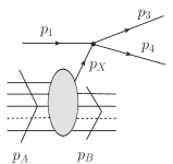
Figure 1: The amplitude of the process $A(p,2p)B$. The lines are marked with four-momenta of the particles: the initial ($p_{A}$) and final ($p_{B}$) nuclei, incident proton ($p_{1}$), struck proton ($p_{X}$), outgoing protons ($p_{3}$ and $p_{4}$).

In the Feynman diagram representation, the amplitude of the studied process is shown in Fig. 1 which gives the following invariant matrix element:

$$M=M_{\rm el}(p_{3},p_{4},p_{1})\frac{i\Gamma_{A\to XB}(p_{A},p_{B})}{p_{X}^{2}-m^{2}+i\epsilon}~{},$$ (1)

where $M_{\rm el}(p_{3},p_{4},p_{1})$ is the invariant matrix element of elastic $pp$ scattering amplitude, $\Gamma_{A\to XB}(p_{A},p_{B})$ is the nuclear virtual decay vertex, and $m$ is the nucleon mass. The sum over all intermediate state quantum numbers is implicitly assumed in Eq.(1). For the residual nucleus $B$ on the mass shell, in the rest frame (r.f) of the initial nucleus $A$, the decay vertex can be expressed as follows:

$$\frac{i\Gamma_{A\to XB}(p_{A},p_{B})}{p_{X}^{2}-m^{2}+i\epsilon}=S_{A}^{X}\left(\frac{2E_{B}m_{A}}{p_{X}^{0}}\right)^{1/2}(2\pi)^{3/2}\psi_{nl}^{m_{l}}(-\boldsymbol{p}_{X})~{},$$ (2)

where $\psi_{nl}^{m_{l}}(-\boldsymbol{p}_{X})$ is the WF of the relative motion of the struck proton $X$ and the nucleus $B$ in momentum space with $n$ being the HO main quantum number, $l$ – the relative orbital momentum, and $m_{l}$ – the magnetic quantum number. The WF is normalized as follows:

$$\int d^{3}p_{X}|\psi_{nl}^{m_{l}}(-\boldsymbol{p}_{X})|^{2}=1~{}.$$ (3)

$S_{A}^{X}$ is the spectroscopic amplitude, i.e. the virtual decay amplitude $A\to XB$ expressed via the overlap integral of the WF of the nucleus $A$ and the antisymmetrized product of the WF of the nucleus $B$ and the relative WF of the proton $X$ and nucleus $B$ Smirnov and Tchuvil’sky (1977); Uzikov and Uvarov (2022):

$$S_{A}^{X}([f]LSTJMM_{T};[f_{B}]L_{B}S_{B}T_{B}J_{B}M_{B}M_{T_{B}};m_{l},\sigma)=A^{1/2}\langle\Psi_{A}|\Psi_{B},nl\rangle$$ (8)

$$= A^{1/2}\sum_{J_{0}M_{0}}\left\{\begin{array}[]{lll}L_{B}&S_{B}&J_{B}\\ l&1/2&J_{0}\\ L&S&J\end{array}\right\}\sqrt{(2L+1)(2S+1)(2J_{B}+1)(2J_{0}+1)}$$

$$\times\langle AN[f]LST|(A-1)N_{B}[f_{B}]L_{B}S_{B}T_{B};nl\rangle$$

$$\times(J_{B}M_{B}J_{0}M_{0}|JM)\,(lm_{l}\frac{1}{2}\sigma|J_{0}M_{0})\,(T_{B}M_{T_{B}}\frac{1}{2}\tau|TM_{T})~{},$$

where the internal WF of the initial nucleus $|\Psi_{A}\rangle\equiv|AN[f]LSTJMM_{T}\rangle$ is determined by $N$ – the number of the oscillator quanta, $[f]$ – the Young scheme, $L$, $S$, $J$ – the orbital, spin, and total angular momenta, respectively, $T$ – isospin, $M$ and $M_{T}$ – $z$-components of $J$ and $T$, respectively. The internal WF of the final nucleus is determined by similar quantum numbers $|\Psi_{B}\rangle\equiv|(A-1)N_{B}[f_{B}]L_{B}S_{B}T_{B}J_{B}M_{B}M_{T_{B}}\rangle$. The state of the struck nucleon $X$ is determined by the spin, $\sigma$, and isospin, $\tau$, projections. The numbers of oscillator quanta satisfy the sum rule $N=N_{B}+n$. For the WF of relative $X-B$ motion with quantum numbers $n=l=1$, the one-particle fractional parentage coefficient (FPC) of the TISM (the term in the angular brackets in Eq.(8)) can be expressed via the FPC of the conventional shell model as follows Smirnov and Tchuvil’sky (1977):

$$\langle AN[f]LST|(A-1)N_{B}[f_{B}]L_{B}S_{B}T_{B};11\rangle$$

$$=-\left(\frac{A-4}{A-1}\right)^{1/2}\langle p^{A-4}[f]LST|p^{A-5}[f_{B}]L_{B}S_{B}T_{B}\rangle~{}.$$ (9)

The FPC of the conventional shell model can be calculated in a standard way from the tables of Ref. Jahn and van Wieringen (1951) taking into account the correction of phases of some orbital WFs as mentioned in the footnote of Ref. Elliott et al. (1953).

Equation (2) assumes transition from a TISM state of the nucleus $A$ to a TISM state of the nucleus $B$. Eigenstates of a realistic nuclear Hamiltonian should be the superposition of TISM states. This means that actual spectroscopic amplitude for the transition between the physical states of the nuclei $A$ and $B$ is obtained by the weighted sum

$$\sum_{i,j}\alpha_{i}\beta_{j}^{*}S_{A}^{X}([f_{i}]L_{i}S_{i}T_{i}JMM_{T};[f_{j}]L_{j}S_{j}T_{j}J_{B}M_{B}M_{T_{B}};m_{l},\sigma)\equiv S_{A}^{X}(JMM_{T};J_{B}M_{B}M_{T_{B}};m_{l},\sigma)~{},$$ (10)

where the indices $i$ and $j$ enumerate the TISM states which enter the decomposition of the physical states of the nuclei $A$ and $B$, respectively. The corresponding partial amplitudes $\alpha_{i}$ and $\beta_{j}$ are model dependent. We will apply the intermediate coupling model of Ref. Boyarkina (1973) which produces the real-valued partial amplitudes listed for ¹²C ground state in Table 1, and for ¹¹B ground state and two excited states in Table 2.

Table 1: Contributing $(1p)^{8}$ TISM states denoted as $[f]^{(2T+1)(2S+1)}L$ with their partial amplitudes for the ¹²C ground state ($J=T=0$). Taken from Ref. Boyarkina (1973).

$[44]^{11}S$	$[431]^{13}P$	$[422]^{11}S$	$[422]^{15}D$	$[332]^{13}P$
0.840	0.492	0.064	-0.200	0.086

Table 2: Same as in Table 1 but for $(1p)^{7}$ TISM states in ¹¹B. The ground state and two excited states are included. The values of excitation energy are experimental ones. Taken from Ref. Boyarkina (1973).

$E^{*}=0$ MeV, $T=1/2,J=3/2$ $[43]^{22}P$ $[43]^{22}D$ $[421]^{22}P$ $[421]^{24}P$ $[421]^{22}D$ $[421]^{24}D$ $[421]^{24}F$ 0.636 0.566 -0.223 -0.168 -0.087 -0.309 0.198 $[331]^{24}S$ $[331]^{22}D$ $[331]^{24}D$ $[322]^{22}P$ $[322]^{24}P$ $[322]^{26}P$ 0.158 0.123 0.043 -0.016 0.080 0.080

$E^{*}=2.13$ MeV, $T=1/2,J=1/2$

$[43]^{22}P$	$[421]^{22}P$	$[421]^{24}P$	$[421]^{24}D$	$[331]^{22}S$	$[331]^{24}D$	$[322]^{22}P$	$[322]^{24}P$
0.913	0.161	-0.132	-0.314	0.126	-0.088	0.000	0.001

$E^{*}=5.02$ MeV, $T=1/2,J=3/2$

$[43]^{22}P$	$[43]^{22}D$	$[421]^{22}P$	$[421]^{24}P$	$[421]^{22}D$	$[421]^{24}D$	$[421]^{24}F$
-0.532	0.721	-0.061	0.207	0.272	0.036	0.079
$[331]^{24}S$	$[331]^{22}D$	$[331]^{24}D$	$[322]^{22}P$	$[322]^{24}P$	$[322]^{26}P$
-0.166	0.021	0.155	0.048	-0.039	-0.111

So far we discussed the case of IA neglecting ISI/FSI. We will now include the ISI/FSI in the eikonal approximation, similar to Ref. Larionov and Uzikov (2023). This is reached by replacing in Eq. (2)

$$(2\pi)^{3/2}\psi_{nl}^{m_{l}}(-\boldsymbol{p}_{X})\to\int d^{3}r\mbox{e}^{-i\boldsymbol{p}_{X}\boldsymbol{r}}\psi_{nl}^{m_{l}}(-\boldsymbol{r})F_{1}(\boldsymbol{r})F_{3}(\boldsymbol{r})F_{4}(\boldsymbol{r})\equiv(2\pi)^{3/2}\tilde{\psi}_{nl}^{m_{l}}(-\boldsymbol{p}_{X})~{},$$ (11)

where $\boldsymbol{r}=\boldsymbol{R}_{X}-\boldsymbol{R}_{B}$ is the relative position vector of the struck proton and the center-of-mass (c.m.) of the residual nucleus $B$. Thus, Eq.(11) takes into account nuclear absorption introduced via factors

$$F_{j}(\boldsymbol{r})=\exp\left(-\frac{i}{v_{j}}\int\limits_{-\infty}^{0}d\eta\,U_{j}(\boldsymbol{r}\pm\hat{\boldsymbol{p}}_{j}\eta)\right)~{},$$ (12)

where $v_{j}=p_{j}/E_{j}$ is the $j$-th particle velocity in the rest frame (r.f.) of the nucleus $B$, $\hat{\boldsymbol{p}_{j}}\equiv\boldsymbol{p}_{j}/p_{j}$, and $U_{j}(\boldsymbol{r})$ is the optical potential. In Eq.(12), the integral is taken along the trajectory of the $j$-th particle that corresponds to the “+” sign for $j=1$ (incoming proton) and “-” sign for $j=3,4$ (outgoing protons). At relativistic energies, in good approximation, the latter can be expressed as follows:

$$U_{j}(\boldsymbol{r})=-\frac{i}{2}v_{j}\sigma_{NN}(p_{j})\rho(\boldsymbol{r})~{},$$ (13)

where $\sigma_{NN}(p_{j})$ is the total $NN$ cross section, and $\rho(\boldsymbol{r})$ is the nucleon number density of the nucleus $B$ in the point $\boldsymbol{r}$. The resulting absorption factors are then essentially similar to those in the Glauber approximation Van Overmeire et al. (2006).

We will consider the case of unpolarized particles and, thus, the matrix element modulus squared should be averaged over spin magnetic quantum numbers of the initial particles and summed over those of final particles:

$$\overline{|M|^{2}} \equiv \frac{1}{2(2J+1)}\sum_{\sigma_{1},\sigma_{3},\sigma_{4},M,M_{B}}|M|^{2}$$ (14)

$$= \frac{1}{2(2J+1)}\sum_{\sigma_{1},\sigma_{3},\sigma_{4},M,M_{B}}\sum_{\sigma,\sigma^{\prime}}\sum_{m_{l},m_{l}^{\prime}}M_{\rm el}(p_{3},p_{4},p_{1};\sigma_{3},\sigma_{4},\sigma_{1},\sigma)M_{\rm el}^{*}(p_{3},p_{4},p_{1};\sigma_{3},\sigma_{4},\sigma_{1},\sigma^{\prime})$$

$$\times\frac{2E_{B}m_{A}}{p_{X}^{0}}(2\pi)^{3}\tilde{\psi}_{11}^{m_{l}}(-\boldsymbol{p}_{X})\tilde{\psi}_{11}^{m_{l}^{\prime}*}(-\boldsymbol{p}_{X})$$

$$\times S_{A}^{X}(JMM_{T};J_{B}M_{B}M_{T_{B}};m_{l},\sigma)S_{A}^{X*}(JMM_{T};J_{B}M_{B}M_{T_{B}};m_{l}^{\prime},\sigma^{\prime})~{},$$

where we explicitly included summations over intermediate state quantum numbers $\sigma,\sigma^{\prime},m_{l},m_{l}^{\prime}$. To simplify Eq.(14), we, first, neglect the interference terms with $\sigma^{\prime}\neq\sigma$ and replace

$$\frac{1}{2}\sum_{\sigma_{1},\sigma_{3},\sigma_{4}}|M_{\rm el}(p_{3},p_{4},p_{1};\sigma_{3},\sigma_{4},\sigma_{1},\sigma)|^{2}$$

$$\to\overline{|M_{\rm el}(p_{3},p_{4},p_{1})|^{2}}\equiv\frac{1}{4}\sum_{\sigma_{1},\sigma_{3},\sigma_{4},\sigma}|M_{\rm el}(p_{3},p_{4},p_{1};\sigma_{3},\sigma_{4},\sigma_{1},\sigma)|^{2}~{}.$$ (15)

Then, after somewhat lengthy but straightforward derivation we come to the following expression:

$$\overline{|M|^{2}} = \overline{|M_{\rm el}(p_{3},p_{4},p_{1})|^{2}}\,\frac{2E_{B}m_{A}}{p_{X}^{0}}(2\pi)^{3}\,\overline{|\tilde{\psi}_{11}(-\boldsymbol{p}_{X})|^{2}}\,S~{},$$ (16)

where

$$\overline{|\tilde{\psi}_{11}(-\boldsymbol{p}_{X})|^{2}}\equiv\frac{1}{3}\sum_{m_{l}=-1}^{1}|\tilde{\psi}_{11}^{m_{l}}(-\boldsymbol{p}_{X})|^{2}~{}.$$ (17)

The spectroscopic factor in Eq.(16) is expressed as follows:

$$S = A\,(T_{B}M_{T_{B}}\frac{1}{2}\tau|TM_{T})^{2}\,(2J_{B}+1)\,\sum_{J_{0}}(2J_{0}+1)\,|\sum_{i,j}\alpha_{i}\beta_{j}^{*}\left\{\begin{array}[]{lll}L_{j}&S_{j}&J_{B}\\ 1&1/2&J_{0}\\ L_{i}&S_{i}&J\end{array}\right\}$$ (22)

$$\times\sqrt{(2L_{i}+1)(2S_{i}+1)}\,\langle AN[f_{i}]L_{i}S_{i}T|(A-1)N_{B}[f_{j}]L_{j}S_{j}T_{B};11\rangle|^{2}~{}.$$

Equation (17) for the modulus squared of the ISI/FSI-corrected WF is quite involved but can be simplified. Substituting Eq.(11) in Eq.(17) we have:

$$\overline{|\tilde{\psi}_{11}(-\boldsymbol{p}_{X})|^{2}} = \frac{1}{3(2\pi)^{3}}\sum_{m_{l}}\int d^{3}r\int d^{3}r^{\prime}\mbox{e}^{-i\boldsymbol{p}_{X}(\boldsymbol{r}-\boldsymbol{r}^{\prime})}\psi_{11}^{m_{l}}(-\boldsymbol{r})\psi_{11}^{m_{l}*}(-\boldsymbol{r}^{\prime})F_{\rm abs}(\boldsymbol{r})F_{\rm abs}(\boldsymbol{r}^{\prime})$$ (23)

$$\simeq \frac{1}{(2\pi)^{3}}\int d^{3}R\,f_{11}(-\boldsymbol{R},-\boldsymbol{p}_{X})F_{\rm abs}^{2}(\boldsymbol{R})~{},$$

where $F_{\rm abs}(\boldsymbol{r})\equiv F_{1}(\boldsymbol{r})F_{3}(\boldsymbol{r})F_{4}(\boldsymbol{r})$ is the absorption factor, and

$$f_{11}(-\boldsymbol{R},-\boldsymbol{p}_{X})\equiv\frac{1}{3}\sum_{m_{l}}\int d^{3}\xi\mbox{e}^{-i\boldsymbol{p}_{X}\boldsymbol{\xi}}\,\psi_{11}^{m_{l}}(-\boldsymbol{R}-\boldsymbol{\xi}/2)\psi_{11}^{m_{l}\,*}(-\boldsymbol{R}+\boldsymbol{\xi}/2)$$ (24)

is a Wigner function. In Eq.(23), in the last step, we introduced variables $\boldsymbol{R}\equiv(\boldsymbol{r}+\boldsymbol{r}^{\prime})/2$, $\boldsymbol{\xi}\equiv\boldsymbol{r}-\boldsymbol{r}^{\prime}$ and approximately set $\boldsymbol{\xi}=0$ in the product of absorption factors $F_{\rm abs}(\boldsymbol{R}+\boldsymbol{\xi}/2)F_{\rm abs}(\boldsymbol{R}-\boldsymbol{\xi}/2)$ (see Ref. Larionov and Uzikov (2023) for discussion of validity of this approximation).

The TISM WF of the relative $X-B$ motion is

$$\psi_{11}^{m_{l}}(-\boldsymbol{R})=\left(\frac{8}{3\pi^{1/2}R_{0}^{5}}\right)^{1/2}R\,\mbox{e}^{-R^{2}/2R_{0}^{2}}\,Y_{1m_{l}}(-\hat{\boldsymbol{R}})~{},$$ (25)

where $R_{0}=r_{0}[A/(A-1)]^{1/2}$, and $r_{0}=1.581$ fm is the parameter of the conventional HO shell model Alkhazov et al. (1972). The Wigner function (24) can be then easily calculated:

$$f_{11}(-\boldsymbol{R},-\boldsymbol{p}_{X})=8\,\mbox{e}^{-(R^{2}+p_{X}^{2}R_{0}^{4})/R_{0}^{2}}\left[\frac{2}{3R_{0}^{2}}(R^{2}+p_{X}^{2}R_{0}^{4})-1\right]~{}.$$ (26)

This expression can be used in Eq.(23) for numerical calculations of $\overline{|\tilde{\psi}_{11}(-\boldsymbol{p}_{X})|^{2}}$ taking into account ISI/FSI. In the case of IA, one recovers an analytical formula:

$$\overline{|\psi_{11}(-\boldsymbol{p}_{X})|^{2}}=\frac{2R_{0}^{5}}{3\pi^{3/2}}\,p_{X}^{2}\,\mbox{e}^{-p_{X}^{2}R_{0}^{2}}~{}.$$ (27)

The invariant matrix element of elastic $pp$ scattering is related to the differential cross section by a standard formula:

$$\frac{d\sigma_{\rm el}}{dt}=\frac{\overline{|M_{\rm el}(t,s)|^{2}}}{64\pi I_{pp}^{2}}~{},$$ (28)

where $I_{pp}=\sqrt{(s/4-m^{2})s}$ is the flux factor, $s=(p_{3}+p_{4})^{2}$, $t=\max\{(p_{1}-p_{3})^{2},(p_{1}-p_{4})^{2}\}$. By using the high-energy parameterization $d\sigma_{\rm el}/dt\propto\mbox{e}^{bt}$ one obtains the following relation:

$$\overline{|M_{\rm el}(t,s)|^{2}}=64\pi I_{pp}^{2}\,\frac{b\sigma_{\rm el}}{1-\mbox{e}^{bt_{0}}}\,\mbox{e}^{bt}~{},$$ (29)

where $t_{0}=-2(s/4-m^{2})$. The experimental integrated elastic $pp$ cross section, $\sigma_{\rm el}$, and the slope parameter, $b$, are conveniently parameterized in Ref. Cugnon et al. (1996) as functions of the beam momentum, $p_{\rm lab}=I_{pp}/m$, for $p_{\rm lab}\raisebox{-2.15277pt}{$\>\stackrel{{\scriptstyle\textstyle<}}{{\sim}}\>$}5-6$ GeV/c.

For the calculation of the optical potential, Eq.(13), one has to specify the total $pN$ cross section and the nucleon density distribution. We apply the proton/neutron-number-weighted formula

$$\sigma_{pN}=[\sigma_{pp}Z_{B}+\sigma_{pn}(A_{B}-Z_{B})]/A_{B}~{},$$ (30)

where $\sigma_{pp}$ and $\sigma_{pn}$ are, respectively, the total $pp$ and $pn$ cross sections in the parameterizations of Ref. Cugnon et al. (1996) that provide good fits of available experimental data at $p_{\rm lab}\raisebox{-2.15277pt}{$\>\stackrel{{\scriptstyle\textstyle<}}{{\sim}}\>$}3-5$ GeV/c. $A_{B}=A-1$ and $Z_{B}=Z-1$ are, respectively, the mass and charge numbers of the residual nucleus $B$. The nucleon density distribution in the nucleus with $A_{B}$ nucleons in the $s^{4}p^{A_{B}-4}$ configuration is described by the conventional HO shell model formula

$$\rho(r)=\frac{4}{r_{0}^{3}\pi^{3/2}}\left[1+\frac{A_{B}-4}{6}\left(\frac{r}{r_{0}}\right)^{2}\right]\mbox{e}^{-r^{2}/r_{0}^{2}}~{}.$$ (31)

The fully differential cross section of the process $A(p,2p)B$ (see Fig. 1 for notation) is expressed as follows:

$$d\sigma_{1A\to 34B}=\frac{(2\pi)^{4}\overline{|M|^{2}}}{4I_{pA}}\delta^{(4)}(p_{1}+p_{A}-p_{3}-p_{4}-p_{B})\frac{d^{3}p_{3}}{(2\pi)^{3}2E_{3}}\frac{d^{3}p_{4}}{(2\pi)^{3}2E_{4}}\frac{d^{3}p_{B}}{(2\pi)^{3}2E_{B}}~{},$$ (32)

where $I_{pA}=p_{\rm beam}m$ is the flux factor, $p_{\rm beam}$ is the momentum of the nucleus $A$ in the r.f. of the proton 1 which will be called “laboratory frame” below.. The experiment of Ref. Panin et al. (2016) has been performed at $p_{\rm beam}/A=0.951$ GeV/c where the $pp$ elastic cross section is almost isotropic in the effective region of integration over transferred rescattering momentum in the c.m. frame as follows from the used here parameterization Cugnon et al. (1996).

Thus, it is convenient to perform the integration over invariants $d^{3}p_{3}/E_{3}$ and $d^{3}p_{4}/E_{4}$ in the c.m. frame of the protons 3 and 4. On the other hand, the matrix element is proportional to the WF of the relative $X-B$ motion which suppresses large absolute values of the momentum $\boldsymbol{p}_{B}$ of the residual nucleus in the r.f. of the nucleus $A$. Thus, the integration over invariant $d^{3}p_{B}/E_{B}$ is reasonable to perform in the r.f. of the nucleus $A$. As a result, we come to the following expression for the integrated cross section:

$$\sigma_{1A\to 34B}=\frac{1}{32(2\pi)^{5}p_{\rm beam}m}\int\frac{d^{3}p_{B}}{\sqrt{p_{B}^{2}+m_{B}^{2}}}\int\frac{p_{3}d\Omega_{3}}{2\sqrt{p_{3}^{2}+m^{2}}}\overline{|M|^{2}}~{},$$ (33)

where the momentum $\boldsymbol{p}_{B}$ is defined in the r.f. of the nucleus $A$ while the momentum $\boldsymbol{p}_{3}$ and the corresponding solid angle element $d\Omega_{3}$ – in the c.m. frame of the protons 3 and 4. Due to identity of the differential cross section with respect to the interchange of momenta of the 3-d and 4-th protons, the integration over $d\Omega_{3}$ should be performed over the solid angle hemisphere of $2\pi$ (the orientation of the hemisphere does not play a role). Due to rotational symmetry about the beam axis, it is also possible to reduce the integration order by writing in the spherical coordinates with $z$-axis along the 1-st proton momentum in the r.f. of $A$ $d^{3}p_{B}=p_{B}^{2}dp_{B}2\pi d\Theta_{B}$ and perform all integrations in Eq.(33) with arbitrarily fixed value of the azimuthal angle $\phi_{B}$. Finally, the differential cross sections, $d\sigma_{1A\to 34B}/dx$, where $x$ is any kinematic variable determined by the momenta ${\bf p}_{3}$ and ${\bf p}_{B}$, are evaluated by multiplying the integrand of Eq.(33) by the factor $\delta[x-x(\boldsymbol{p}_{B},\boldsymbol{p}_{3})]$.

3 Results

The integrated cross sections are listed in Table 3. One can see from this Table that absorption reduces all partial cross section by a factor of 5.1 but does not change the ratios between the partial cross sections for different states of ¹¹B. The experimental total cross section is reproduced by full calculation surprisingly well, with accuracy of about $3\%$. The strong dominance of ¹¹B production in the ground state is also correctly reproduced. Discrepancies for excited states are quite large. However, this is still satisfactory given the fact that we did not introduce any additional model parameters (like phenomenological spectroscopic factors, see discussion section) to tune our calculations.

Table 3: Integrated cross sections of the process ${}^{12}\mbox{C}(p,2p)^{11}\mbox{B}$ with 400 MeV/nucleon ¹²C beam for the ground state and two excited states of the residual nucleus ${}^{11}\mbox{B}$. Listed are the results of full calculations (including absorption), calculations in the IA, and the spectroscopic factors calculated using Eq.(22). Experimental data are from Ref. Panin et al. (2016). Total errors are given in parentheses.

$E^{*}$ (MeV)	$J^{\pi}$	$\sigma_{\rm exp}$ (mb)	$\sigma_{\rm full}$ (mb)	$\sigma_{\rm IA}$ (mb)	$S$
0.0 (G.S.)	$3/2^{-}$	$15.8(18)$	12.3	62.6	2.82
2.13	$1/2^{-}$	$1.9(2)$	2.9	14.9	0.67
5.02	$3/2^{-}$	$1.5(2)$	3.4	17.5	0.79
Total:		$19.2(3)$	18.6	95.0	4.28

Fig. 2 shows the distribution of opening angle, $\Theta_{\rm opening}=\arccos(\boldsymbol{p}_{3}\boldsymbol{p}_{4}/p_{3}p_{4})$, between outgoing protons in the laboratory frame. The full calculation correctly describes the peak position at $80\degree$ and the distribution at smaller angles, although gives a sharper peak and steeper fall-off at larger angles. The full calculation is slightly shifted to larger opening angles as compared to the calculation in the IA.

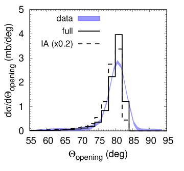
Figure 2: The distribution of opening angle between outgoing protons in the laboratory frame for the process ${}^{12}\mbox{C}(p,2p)^{11}\mbox{B}$ at 400 MeV/nucleon. Solid and dashed histograms show, respectively, the full calculation and the calculation without absorption scaled by a factor of 0.2. The band represents experimental data from Ref. Panin et al. (2016).

Fig. 3 shows the distribution of relative azimuthal angle, $\Delta\phi=\arccos(\boldsymbol{p}_{3t}\boldsymbol{p}_{4t}/p_{3t}p_{4t})$, between the transverse momenta $\boldsymbol{p}_{3t}$ and $\boldsymbol{p}_{4t}$ of outgoing protons. The absorptive ISI/FSI suppress the yield at large deviations of $\Delta\phi$ from $180\degree$ leading to a sharper peak at $\Delta\phi=180\degree$ and better agreement with experiment.

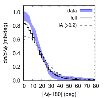
Figure 3: The distribution of the relative azimuthal angle between transverse momenta of outgoing protons for ${}^{12}\mbox{C}(p,2p)^{11}\mbox{B}$ at 400 MeV/nucleon. Line notations are the same as in Fig. 2. The band represents experimental data from Ref. Panin et al. (2016).

Figs. 4,5 and 6 show, respectively, the transverse, longitudinal, and total momentum distributions of the residual nucleus. Absorption leads to the depletion of the yield at large transverse and total momenta shifting the maxima of the $P_{\rm tr}$- and $P_{\rm tot}$ distributions to smaller momenta. This can be understood as follows. In the presence of absorption, the main contribution to the integral in Eq.(23) comes from nuclear periphery (surface ring), since the absorption factor suppresses the integrand deeply inside the nucleus. If the transverse momentum of the residual nucleus is small, then the absorption is in average smaller because both outgoing protons may have small transverse momenta balancing each other and their trajectories avoid the bulk of the nuclear medium. If the transverse momentum of the residual nucleus is large, then at least one of the outgoing protons will have large transverse momentum and, thus, its trajectory will pass through the bulk of the nuclear medium with a larger probability which makes absorption stronger. This is also in-line with stronger absorption at larger deviations of $\Delta\phi$ from $180\degree$ (Fig. 3).

A particular form of the Wigner density for the $n=l=1$ valence nucleon, Eq.(26), acts in the same direction. At small values of $R$ and $p_{X}(=P_{\rm tot})$, the Wigner density becomes negative. It means that absorption should then lead to the enhancement of production which is visible at small values of $P_{\rm tot}$ in Fig. 6.

In the IA calculation, the longitudinal momentum distribution (Fig. 5) is shifted to positive $P_{\rm||}$. This corresponds to the struck proton $X$ moving opposite to the incoming proton 1 in the r.f. of ¹²C giving a larger two-body phase space volume of the protons 3 and 4 (the term $\propto p_{3}/\sqrt{p_{3}^{2}+m^{2}}$ in Eq.(33)). However, with absorption, the $P_{\rm||}$ distribution becomes almost symmetric with respect to the change $P_{\rm||}\to-P_{\rm||}$. This is a consequence of larger average transverse momenta of the 3-d and 4-th protons at $P_{\rm||}>0$ leading to their stronger absorption. This observation also explains the stronger absorption at smaller opening angles (Fig. 2).

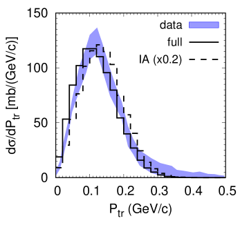
Figure 4: The distribution of the transverse momentum of the residual nucleus for ${}^{12}\mbox{C}(p,2p)^{11}\mbox{B}$ at 400 MeV/nucleon. Line notations are the same as in Fig. 2. The band represents experimental data from Ref. Panin et al. (2016).

Figure 5: The distribution of the longitudinal momentum of the residual nucleus in the r.f. of ¹²C for ${}^{12}\mbox{C}(p,2p)^{11}\mbox{B}$ at 400 MeV/nucleon. Positive values of $P_{\parallel}$ correspond to the direction of the momentum of the incoming proton. Line notations are the same as in Fig. 2.

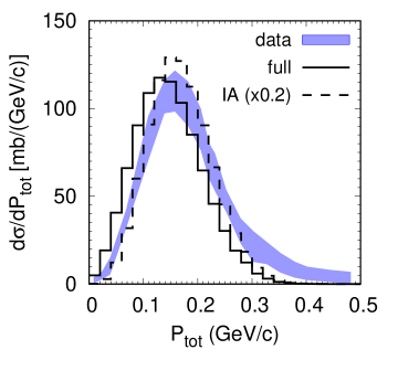
Figure 6: The distribution of the total momentum of the residual nucleus in the r.f. of ¹²C for ${}^{12}\mbox{C}(p,2p)^{11}\mbox{B}$ at 400 MeV/nucleon. Line notations are the same as in Fig. 2. The band represents experimental data from Ref. Panin et al. (2016).

4 Discussion

Table 4 contains results of several other calculations of the spectroscopic factors for the separation of a nucleon from ¹²C in comparison with our results.

Table 4: Spectroscopic factors for the ${}^{12}\mbox{C}\to p^{11}\mbox{B}(n^{11}\mbox{C})$ process calculated in different theoretical models.

$E^{*}$ (MeV)	$J^{\pi}$	Cohen and Kurath (1967)	Singh et al. (1973)	Li et al. (2022)	this work
0.0 (G.S.)	$3/2^{-}$	2.85	3.27	2.50	2.82
2.13	$1/2^{-}$	0.75	0.60	0.48	0.67
5.02	$3/2^{-}$	0.38	0.12		0.79
Total:		3.98	3.99	2.98	4.28

The approach of Ref. Cohen and Kurath (1967) is based on the FPCs of the conventional shell model but in other aspects is quite close to the intermediate coupling model of Refs. Balashov et al. (1964); Boyarkina (1973) applied in our work. In Ref. Singh et al. (1973), the WFs of deformed HO shell model were used without residual interaction taking $K=0$ for ¹²C and $K=1/2,3/2$ for ¹¹B. (In the spherical HO model this corresponds to considering only the Young scheme $[44]$ for ¹²C and $[43]$ for ¹¹B.) In Ref. Li et al. (2022), the no-core shell model was employed in the HO basis with c.m. correction, although the authors state that the dependence of their results on the chosen basis is small. According to Ref. Rodkin and Tchuvil’sky (2021), however, the “old” definition of the spectroscopic amplitude (c.f. our Eq.(8)) relies on the non-normalized WF of the final state and, thus, should be corrected.

Comparison with experimental data for the QE $(p,pN)$ processes depends not only on the spectroscopic factors but also on the ISI/FSI used. In phenomenological DWIA approaches Devins et al. (1979); Aumann et al. (2013), the spectroscopic factor is used as a free parameter to fit experimental cross sections for some fixed ISI/FSI. The latter includes in-medium effects due to Pauli blocking of $NN$ scattering Bertulani and De Conti (2010) (i.e. the antisymmetrization of the full WF of the scattered nucleon and residual nucleus) which can be effectively described by in-medium reduced $NN$ cross sections. It was shown Bertulani and De Conti (2010), that in heavy-ion induced stripping reactions on nuclear targets at $E_{\rm lab}=5-300$ MeV/nucleon, the in-medium effects lead to about 10% change in the nucleon knockout cross sections and momentum distributions. In $(p,pN)$ processes, the in-medium effects are expected to be of the same order or smaller. The in-medium effects should decrease with increasing beam energy rendering Glauber model more natural at $E_{\rm lab}>1$ GeV/nucleon Van Overmeire et al. (2006). Thus, our description of ISI/FSI within Glauber model should be taken with some reservations for possible in-medium corrections.

5 Summary

Based on the TISM, we developed the model for description of fully exclusive $A(p,pp)(A-1)$ reactions at intermediate relativistic energies. The model allows to calculate spectroscopic factors directly from the overlap integral of the WFs. Having in mind future model applications at NICA and FAIR energies, we restricted ourselves to the Glauber model description of the ISI/FSI. As a test case, the model was applied to the reaction ${}^{12}\mbox{C}(p,2p)^{11}\mbox{B}$ at 400 MeV/nucleon measured at GSI Panin et al. (2016) in the inverse kinematics.

The model slightly underestimates the measured integrated cross section for ${}^{11}\mbox{B}$ $3/2^{-}$ ground state, but overpredicts the integrated cross sections for the two excited $1/2^{-}$ and $3/2^{-}$ states. The total integrated cross section for the production of all three ${}^{11}\mbox{B}$ states is well reproduced, however.

The distributions of the outgoing proton pair in the opening angle and relative azimuthal angle, as well as the momentum distributions of the residual nucleus, are reproduced reasonably well. Some deficiency in the production of high-momentum residual nuclei can be attributed to the longitudinal momenta mostly and is probably due to the limited HO WF basis.

Last but not least, the present calculation also puts on a firm ground our previous study of the ${}^{12}\mbox{C}(p,2pN_{s})^{10}\mbox{A}$ exclusive reactions at 48 GeV/c Larionov and Uzikov (2023), where a similar approach has been used.