A Fully-discrete Semi-Lagrangian scheme
for a price formation MFG model

Abstract.

Here, we examine a fully-discrete Semi-Lagrangian scheme for a mean-field game price formation model. We show that the discretization is monotone as a multivalued operator and prove the uniqueness of the discretized solution. Moreover, we show that the limit of the discretization converges to the weak solution of the continuous price formation mean-field game using monotonicity methods. This scheme performs substantially better than standard methods by giving reliable results within a few iterations, as several numerical simulations and comparisons at the end of the paper illustrate.

1. Introduction

This paper investigates first-order price formation mean field games (MFGs), modeling interactions within large populations of agents. Mean field game theory, pioneered by [18, 19] and [17, 16], extends classical optimal control problems to scenarios involving large populations of interacting agents. The price formation problem draws on both optimal control principles [11] and mean-field game techniques to model how individual decisions and market-wide dynamics influence each other.

Price formation MFGs hold the potential to revolutionize how we understand and predict market behavior. By capturing the interactions of many agents, these models can contribute to more efficient resource allocation, improved market stability, and better-informed decision-making for individuals and policymakers. Here, we develop a numerical method for approximating solutions of price formation MFGs using Semi-Lagrangian (SL) schemes.

We consider the following price formation problem.

Problem 1.

Given initial distribution $\bar{m}\in\mathcal{P}(\mathbb{R})$, where $\mathcal{P}(\mathbb{R})$ is the space of probability measures on $\mathbb{R}$, terminal cost $\bar{u}\in C^{2}(\mathbb{R})$, and supply $Q\in C^{2}([0,T])$, and a uniformly convex Hamiltonian, $H\in C^{1}(\mathbb{R}^{2})$. Find functions $u,m:\mathbb{R}\times[0,T]\rightarrow\mathbb{R}$ wwith $m\geq 0$, and $\varpi:[0,T]\rightarrow\mathbb{R}$, satisfying

$$\begin{cases}-u_{t}(x,t)+H(x,\varpi(t)+u_{x}(x,t))=0,&\quad(x,t)\in\mathbb{R}\times[0,T]\\ m_{t}(x,t)-\big{(}D_{p}H(x,\varpi(t)+u_{x}(x,t))m(x,t)\big{)}_{x}=0,&\quad(x,t)\in\mathbb{R}\times[0,T],\\ -\int_{\mathbb{R}}D_{p}H(x,\varpi(t)+u_{x}(x,t))m(x,t)dx=Q(t),&\quad t\in[0,T],\end{cases}$$ (1.1)

subject to initial-terminal conditions

$$\begin{cases}u(x,T)=\bar{u}(x),\qquad x\in\mathbb{R},\\ m(x,0)=\bar{m}(x),\qquad x\in\mathbb{R},\end{cases}$$ (1.2)

In Problem 1, $D_{p}H$ is a partial derivative of $H$ with respect to the second variable. The unknown is the triplet $(u,m,\varpi)$, where the value function, $u$, solves the first equation in the viscosity sense, and the probability distribution of the agents, $m$, solves the second equation in the distributional sense. Finally, the price, $\varpi$, is determined by the balance condition, the third equation in (1.1), which guarantees that supply $Q(t)$ meets demand exactly. A typical agent’s state, represented by $x\in\mathbb{R}$, denotes their assets. At time $t$, the distribution of assets is encoded in the probability measure $m(\cdot,t)$. Every agent trades assets at a price given by the time-dependent function $\varpi(t)$. Section 2 briefly recalls the preceding problem’s derivation and motivation.

Under the assumptions discussed in Section 3, in [11], the authors proved the existence and uniqueness of a solution $(u,m,\varpi)$ to Problem 1. This model assumes deterministic supply, a simplification which aids analysis but limits applicability in scenarios with uncertain supply. Nonetheless, deterministic models offer a foundation for understanding more complex markets and can be directly useful when accurate forecasts are available.

The complexity of these models often renders analytical solutions infeasible. Numerical methods allow for the analysis of richer market dynamics, providing insights into previously unsolvable problems and informing decision-making in practical applications. A significant challenge is the forward-backward nature of traditional MFGs, compounded by the additional balance condition. Researchers have suggested various numerical techniques for solving standard MFG systems; for example, finite difference schemes and Newton-based approaches were presented in [1] and [2], respectively, for standard MFGs without balance conditions. For the specific model considered here, in [5], the authors introduced a potential function that transforms the price formation MFG into a convex variational problem. Using this variational structure, this problem is solved numerically by minimizing a suitable functional discretized with finite differences.

Price problems with a stochastic supply and price were introduced in [14] and [15], respectively. Substantial effort was made to address the issue of common noise with machine learning (ML) techniques. In [13], an ML approach employing dual recurrent neural networks and adversarial training to address the price formation MFG model with common noise is given. An ML training process was developed based on a min-max characterization of control and price variables in [12]. Using the potential transformation, [4] solved the price problem with common noise using a recurrent neural network. These methods are suitable for common noise problems where standard numerical methods fail. However, these methods can be slow for deterministic cases. This was, in fact, one of the original motivations for our work.

Here, in the deterministic case, we develop efficient and accurate methods for deterministic price models. We build on previous work on SL schemes for MFGs. Both semi-discrete and fully discrete SL schemes have been employed for first and second-order MFGs [7], [9], and [8]. In the Hamilton-Jacobi equation, we use a fully discrete SL scheme, and for the transport equation, we use the adjoint of the linearization of the Hamilton-Jacobi equation. For the balance condition, we use a simple numerical quadrature. This discretization and the algorithm to solve it are detailed in Section 4. Properties and estimates related to the discretization are presented in Section 5.

Our approach addresses several key gaps in existing numerical methods for price formation MFG: challenges with computational efficiency, accuracy in nonlinear scenarios, and suitability for large-scale validation of machine learning results. Our SL-based scheme offers advancements in all of these areas: it provides improved computational speed, robust handling of complex market dynamics, and the precision necessary for benchmarking ML models. These advantages are crucial for iterative analysis, policy testing, real-time applications, and the development of reliable, data-driven market insights. A detailed comparison between our fully discrete SL, potential minimization, and ML methods appears in Section 7.

2. Background

This section establishes the foundation for our price formation model. The model examines how prices form within a market where numerous agents interact, each trading motivated by profit maximization (here formulated as cost-minimization). Employing optimal control theory, we analyze how individual agents strategize to minimize costs associated with holding an asset, market impact, storage costs, and risk preferences. Additionally, using mean-field game theory, we track the overall distribution of agents, impacting supply and demand. These individual choices and their aggregate distribution together with a market clearing mechanism form the core mechanism that ultimately drive price dynamics within this model.

Agents have a a state $X(t)\in\mathbb{R}$ which corresponds to the assets they hold. Let $\mathcal{A}_{t}$ be the set of bounded, measurable real-valued functions on the interval $[t,T]$. An admissible control is a function $\alpha\in\mathcal{A}_{t}$. Each agent selects an admissible control which drives its trajectory

$$\begin{cases}dX(s)=\alpha(s)ds,\qquad s\in(t,T),\\ X(t)=x,\end{cases}$$ (2.1)

where $X(t)$ represents the agent’s state at the time $t$. The total cost for an agent is the sum of the terminal cost, $\bar{u}(x)$, and the integral of the running cost, $L(x,t,\alpha)=l_{0}(\alpha)+V(x)+\varpi(t)\alpha(t)$. Here $l_{0}$, the market impact term, represents costs like market impact or other trading expenses. The preference potential, $V(x)$, encodes the agent’s asset level preference and can account for things like storage cost. It can incorporate risk aversion, short-selling constraints, or storage costs. Lastly, $\varpi(t)\alpha(t)$ is the price that agents pay by trading $\alpha$ units at a price $\varpi$. The agent aims to minimize the following cost functional:

$$J(x,t,\alpha)=\int_{t}^{T}L(X(s),s,\alpha(s))ds+\bar{u}(X(T))$$ (2.2)

by selecing appropriate admissible controls.

The value function, $u(x,t)$, is the infimum of the cost functional $J(x,t,\alpha)$ over all $\alpha\in\mathcal{A}_{t}$

$$u(x,t):=\inf_{\alpha\in\mathcal{A}_{t}}.J(x,t,\alpha).$$ (2.3)

The associated Hamiltonian, $H$, is the Legendre-Fenchel transform of $l_{0}+V$, given by

$$H(x,p)=\sup_{\alpha\in\mathbb{R}}\left\{-p\alpha-l_{0}(\alpha)-V(x)\right\}.$$ (2.4)

Viscosity solutions offer a framework to handle potential non-differentiability that arise in such problems [6]. In fact, $u$ is a viscosity solution to the Hamilton-Jacobi equation

$$\begin{cases}-u_{t}(x,t)+H(x,\varpi(t)+u_{x}(x,t))=0,\\ u(x,T)=\bar{u}(x).\end{cases}$$

The dynamic programming principle for (2.3) provides a representation formula for the value function

$$u(x,t-h)=\inf_{\alpha\in\mathcal{A}_{t}}\int_{t-h}^{t}L(X(t-h),t-h,\alpha(s))ds+u(X(t),t),$$ (2.5)

where $X(t)$ solves (2.1). Furthermore, the optimal control $\alpha^{*}$ is given in feedback form by

$$\alpha^{*}(x,t)=-D_{p}H(x,\varpi(t)+u_{x}(x,t)),$$ (2.6)

at all points where $u$ is differentiable.

The transport equation is the adjoint to the linearized Hamilton-Jacobi equation. This transport equation tracks the evolution of the distribution of the states over time and incorporates the initial distribution, $\bar{m}(x)$, as initial condition:

$$\begin{cases}m_{t}(x,t)-\big{(}D_{p}H(x,\varpi(t)+u_{x}(x,t))m(x,t)\big{)}_{x}=0,\\ m(x,0)=\bar{m}(x).\end{cases}$$

More precisely, given $(x,t)\in\mathbb{R}\times[0,T]$, consider the trajectory

$$\Phi_{x,t}(s)=x+\int_{t}^{s}\alpha^{*}(x,r)dr\quad\forall s\in[t,T].$$

We have

$$\begin{cases}d\Phi_{x,t}(s)=\alpha^{*}(\Phi_{x,t}(s),s)ds,\quad\forall s\in(t,T)\\ \Phi_{x,t}(t)=x.\end{cases}$$

Recall that push forward for a probability measure $\mu$ and a map $\psi$, $\psi\#\mu$, is the probability measure defined by

$$\int_{\mathbb{R}}\varphi d(\psi\#\mu)=\int_{\mathbb{R}}\varphi\circ\psi d\mu,$$

for all bounded and continuous functions $\varphi$.

We obtain the density function $m$ from the initial measure $\bar{m}$ by push forward of the flow $\Phi_{\cdot,0}(t)$:

$$m(\cdot,t)=\Phi_{\cdot,0}(t)\#\bar{m}(\cdot).$$

Note that for every $0\leq t\leq t+h\leq T$, we have

$$m(\cdot,t+h)=\Phi_{\cdot,t}(t+h)\#[\Phi_{\cdot,0}(t)\#\bar{m}(\cdot)]=\Phi_{\cdot,t}(t+h)\#m(\cdot,t),$$

that is

$$\int_{\mathbb{R}}\varphi(x)m(x,t+h)dx=\int_{\mathbb{R}}\varphi(\Phi_{x,t}(t+h))m(x,t)dx.$$ (2.7)

Our model presupposes a predefined supply function, denoted by $Q(t)$. The model imposes the equality between supply and demand:

$$\int_{\mathbb{R}}\alpha^{*}(x,t)m(x,t)dx=Q(t).$$ (2.8)

This condition, expressed using the Hamiltonian, becomes

$$-\int_{\mathbb{R}}D_{p}H(x,\varpi(t)+u_{x}(x,t))m(x,t)dx=Q(t).$$ (2.9)

3. Main assumptions

Throughout this paper, we work under the following assumptions as in [11] and ensure that the model is well-posed.

Assumption 1.

Hamiltonian, $H$, is the Legendre-Fenchel transform of a uniformly convex Lagrangian,

$$H(x,p)=\sup_{\alpha\in\mathbb{R}}\left\{-p\alpha-l_{0}(\alpha)-V(x)\right\},$$ (3.1)

where the market impact term, $l_{0}\in C^{2}(\mathbb{R})$, is uniformly convex with a convexity constant $\kappa$; that is, $l_{0}^{{}^{\prime\prime}}(\alpha)\geq\kappa>0$, and the preference potential $V$ is bounded from below.

The assumption that the market impact $l_{0}(\alpha)$ is independent of the agent’s current state $x$ aligns well with price models, where these costs are typically distinct from preference costs $V(x)$. The convexity of $l_{0}$, which penalizes oscillating trading strategies, is fundamental to the stability and uniqueness of the MFG system’s solutions. Without it, the Hamiltonian becomes singular as in (3.1) the supremum could be $+\infty$ if $p\neq 0$.

Assumption 2.

There exist constants $\theta>0$ and $C>0$, such that

$$D^{2}_{pp}H(x,p)>\theta,\qquad|D^{3}_{ppp}H(x,p)|<C,$$

for all $(x,p)\in\mathbb{R}^{2}$.

The uniform convexity of $l_{0}$ yields the strict convexity of $H$ with respect to the second variable and gives an upper bound for $D_{pp}^{2}H$; that is, Assumption 2 implies $|D^{2}_{pp}H(x,p)|<C$. The boundedness of the Hamiltonian’s derivatives is essential for the existence of solutions.

Assumption 3.

The potential $V$, the terminal cost $\bar{u}$, and the initial density $\bar{m}$ belong to $C^{2}(\mathbb{R})$. Furthermore, there exists a constant $C>0$ such that

$$\|V\|_{\mathbb{C}^{2}}\leq C,\quad\|\bar{u}\|_{\mathbb{C}^{2}}\leq C,\quad|\bar{m}^{\prime\prime}|\leq C.$$

Assumption 4.

$V$ and $\bar{u}$ are globally Lipschitz and convex.

The convexity of $V$ and $\bar{u}$ give regularity and uniqueness of solutions, see [11].

Assumption 5.

The supply function, $Q$, belongs to $C^{1}([0,T])$.

The compactness assumption on initial distribution corresponds to the case agent’s assets are bounded for the whole population.

Assumption 6.

The initial distribution function, $\bar{m}$, is compactly supported in $[-\bar{R},\bar{R}]\subset\mathbb{R}$, for some positive number $\bar{R}\in\mathbb{R}$.

Under assumptions 1-5, from [11], we have existence and uniqueness of solution $(u,m,\varpi)$, where $m$ is bounded, $u$ is Lipschitz, semiconcave, and differentiable in $x$. Moreover, from [3], $\varpi$ is Lipschitz continuous. Finally, assumption 6 ensures compact support of the density function $m(x,t)$ up to the terminal time $T$.

4. Discretization

In this section, we construct a discretized version of Problem 1. We use the dynamic programming principle and a fully discrete SL scheme to discretize the value function $u$; for the density function m, we use trajectories of the dynamics (2.1); finally, we discretize the balance condition to get an update rule for the price function $\varpi$. The section concludes by presenting an algorithm to solve the discretized system. In a Semi-Lagrangian scheme, solutions of partial differential equations are approximated by following characteristics. For hyperbolic conservation laws and Hamilton-Jacobi equations, SL schemes are known for their stability and ability to handle sharp gradients or nonsmooth solutions.

To construct the discretization, we introduce the following notations and definitions. Let $\mathbb{R}\subset\mathbb{R}$ be an interval and $T$ a finite time. For given positive numbers $\rho$ and $h$, consider a grid

$$\mathcal{G}_{\rho,h}=\{(x_{i},t_{k})=(i\rho,kh)\,:\,i\in\mathbb{Z},k=0,1,\ldots,N\},$$

such that $t_{N}=Nh=T$.

Consider a set of basis functions $\{\beta_{i}\}_{i\in\mathbb{Z}}$ that consist of compactly supported and infinitely differentiable functions $\beta_{i}\in C^{\infty}_{c}(\mathbb{R})$, each compactly supported in $[x_{i}-\rho,x_{i}+\rho]$, $0\leq\beta_{i}(x)\leq 1$ for $x\in\mathbb{R}$, and $\beta_{i}(x_{j})=\delta_{ij}$, where $\delta_{ij}$ is the Kronecker delta. Furthermore,

$$\sum_{i\in\mathbb{Z}}\beta_{i}(x)=1,\qquad\sum_{i\in\mathbb{Z}}\beta^{\prime}_{i}(x)\leq C^{1}_{\beta}(\rho),\qquad\sum_{i\in\mathbb{Z}}\beta^{\prime\prime}_{i}(x)\leq C^{2}_{\beta}(\rho),$$ (4.1)

for all $x\in\mathbb{R}$, and positive constants $C^{1}_{\beta}(\rho),C^{2}_{\beta}(\rho)$, depending only on $\rho$.

Given values $f(x_{i})$ at the nodes $x_{i}$, we define the interpolation function as

$$I[f](x)=\sum_{i\in\mathbb{Z}}f(x_{i})\beta_{i}(x).$$ (4.2)

This interpolation function is crucial for the Semi-Lagrangian discretization scheme, as it allows for the approximation of a function outside the grid $\mathcal{G}_{\rho,h}$. Moreover our choice of the functions $\beta_{i}$ as a smooth partition of unity, ensures that this approximation is smooth. A well-known estimate (see, e.g., [10, 20]) states that for every bounded Lipschitz function $f$, the following holds:

$$\sup_{x\in\mathbb{R}}\left|I[f](x)-f(x)\right|=O(\rho).$$

Finally, for clarity, we adopt the following notations: for any function $f(x,t)$ and all indices $i\in\mathbb{Z}$, and $k=0,1,\ldots,N$, we denote the value of a function at the node $(x_{i},t_{k})$ by $f_{i,k}$, and the vector $\{f_{i,k}\}_{i\in\mathbb{Z}}$ by $f_{k}$, and for any time-dependent function $g(t)$, $g_{k}:=g(t_{k})$. For any function $f$ we denote its approximation function by $f^{q}$. Because our numerical algorithm is iterative, $f^{q}$ is the approximation of $f$ at $q$-th iteration.

4.1. Hamilton-Jacobi equation

We approximate $u$ by a function $u^{q}$ by replacing the right-hand side of (2.5) with the following Semi-Lagrangian discretization

$$u^{q}(x_{i},t-h)=\inf_{\alpha\in\mathbb{R}}\left\{I[u^{q}(\cdot,t)](y(x_{i},\alpha))+hL(x_{i},t-h,\alpha)\right\},$$ (4.3)

where $y(x,\alpha)=x+h\alpha$ is the discretization of $X(t)$.

For $i\in\mathbb{Z}$ and for $k=N-1,N-2,\ldots,0$ the discrete Hamilton-Jacobi equation is

$$\begin{cases}\displaystyle u^{q}(x_{i},t_{k})=I[u^{q}\lvert_{t=t_{k+1}}](y(x_{i},\alpha^{*q}(x_{i},t_{k})))+hL(x_{i},t_{k},\alpha^{*q}(x_{i},t_{k})),\\ u^{q}(x_{i},t_{N})=\bar{u}(x_{i}).\end{cases}$$ (4.4)

where

$$\alpha^{*q}(x_{i},t_{k}):=\operatorname{arginf}_{\alpha\in\mathbb{R}}\left\{I[u^{q}\lvert_{t=t_{k+1}}](y(x_{i},\alpha))+hL(x_{i},t_{k},\alpha)\right\}.$$ (4.5)

We note that the minimizer in (4.5) may not be unique. This matter can be addressed in one of two ways. Either by the conditions in Lemma 5.3, which ensure the uniqueness of a minimizer, or through the interpretation of the discretized system as a multivalued monotone operator. This last approach is addressed in Section 6. Here, in the remaining of this section, we suppose that $\alpha^{*}$ is unique.

4.2. Continuity equation

The discretization of the Hamilton-Jacobi equation offers a method to approximate the value function. Now, we consider the continuity equation, which complements this, approximating the time evolution of density functions.

Substituting $\varphi(x)$ by $\beta_{i}(x)$ in equation (2.7) , we get

$$\int_{\mathbb{R}}\beta_{i}(x)m(x,t+h)dx=\int_{\mathbb{R}}\beta_{i}(\Phi_{x,t}(t+h))m(x,t)dx.$$

Taking into account that $\beta_{i}(x_{j})=\delta_{ij}$, the preceding expression suggests the discretization formula for $m(x,t)$

$$\begin{cases}m^{q}(x_{i},t_{k+1})=\sum_{j\in\mathbb{Z}}\beta_{i}(\Phi_{x_{j},t_{k}}(t_{k+1}))m^{q}(x_{j},t_{k}),\\ m^{q}(x_{i},t_{0})=\bar{m}(x_{i}),\end{cases}$$ (4.6)

for $i\in\mathbb{Z}$ and $k=1,2,\ldots,N$, where we use the discretized flow given by

$$\Phi_{x_{i},t_{k}}(t_{k+1})=x_{i}+h{\alpha^{*}}^{q}(x_{i},t_{k}).$$

4.3. Balance condition

Here, we address the discretization of the last term in (1.1), the balance condition. This discretization yelds an implicit formula for the price function:

$$-\sum_{i\in\mathbb{Z}}D_{p}H(\varpi^{q+1}_{k}+D_{x}u^{q}_{i,k})m^{q}_{i,k}\Delta x=Q_{k},$$ (4.7)

Notice that, since Hamiltonian is separable; therefore, $D_{p}H$ is a function of $p$ alone. From the feedback formula (2.6) and the definition of $\alpha^{*}$ (4.5), we have

$$D_{x}u^{q}_{i,k}=D_{p}H^{-1}(-\alpha_{i,k}^{*q})-\varpi^{q}_{k}.$$

Substituting into the discretization of the balance condition (4.8), we get an implicit update rule for price, for each iteration $q$,

$$\sum_{i\in\mathbb{Z}}D_{p}H(x,\varpi^{q+1}_{k}-\varpi^{q}_{k}+D_{p}H^{-1}(-\alpha_{i,k}^{*q}))m^{q}_{i,k}\Delta x=-Q_{k},$$ (4.8)

for $k=0,1,\ldots,N-1$.

According to the prior discussion, the discretization of the MFG system (1.1)-(1.2) is represented by the system of equations (4.4), (4.6), and (4.8). We employ an iterative algorithm outlined below to effectively solve this discretized system.

4.4. Algorithm

1. Initialize $q=0$, select an initial guess for the price, $\varpi^{q}$, and fix a tolerance parameter, $\varepsilon>0$.

2. For $k=N-1,N-2,\ldots,0$ and $i\in\mathbb{Z}$, find

   $$\alpha_{i,k}^{*q}=\operatorname{arginf}_{\alpha\in\mathbb{R}}\left\{I[u\lvert_{t=t_{k+1}}](x_{i}+h\alpha)+hL(x_{i},t_{k},\alpha)\right\}$$

   and compute the value function, $u$, using the discretization of the Hamilton-Jacobi equation:

   $$\begin{cases}\displaystyle u^{q}_{i,k}=I[u^{q}\lvert_{t=t_{k+1}}](x_{i}+h\alpha_{i,k}^{*q})+hL(x_{i},t_{k},\alpha_{i,k}^{*q}),\\ u^{q}_{i,N}=\bar{u}_{i}.\end{cases}$$

3. For $k=0,1,\ldots,N-1$ and $i\in\mathbb{Z}$, compute the distribution function, $m^{q}$, using the discretization of the Fokker-Planck equation:

   $$\begin{cases}\displaystyle m^{q}_{i,k+1}=\sum_{j=0}^{M}\beta_{i}\left(x_{j}+h\alpha_{j,k}^{*q}\right)m^{q}_{j,k},\\ m^{q}_{i,0}=\bar{m}_{i}.\end{cases}$$

4. For $k=0,1,\ldots,N-1$, update the price, $q\to q+1$, from the following implicit equation

   $$\sum_{i\in\mathbb{Z}}D_{p}H(x_{i},\varpi^{q+1}_{k}-\varpi^{q}_{k}+D_{p}H^{-1}(-\alpha_{i,k}^{*q}))m^{q}_{i,k}\Delta x=-Q_{k}.$$

5. If

   $$\|\varpi^{q+1}-\varpi^{q}\|_{\infty}<\varepsilon,$$

   stop, otherwise, set $\varpi^{q}:=\varpi^{q+1}$, and repeat steps $1)-4)$.

Observe that the price function is defined up to the $N-1$ time step, since there is no optimization occurs at the terminal time.

To avoid notational clutter, subsequent sections omit the explicit dependence on $q$ for symbols representing approximation functions when the context is clear.

5. Some properties and estimates

This section establishes the theoretical foundation for our discretization scheme. Specifically, we establish several properties crucial to its well-definedness, consistency, and computational behavior. First, we demonstrate the existence and uniqueness of minimizers within the scheme. Next, we derive crucial bounds for the discretized variables, followed by proving that compactly supported initial distributions remains compactly supported.

Let the right-hand side of the value function discretization in (4.4) be denoted by

$$S_{\rho,h}(f,i,k):=\inf_{\alpha\in\mathbb{R}}\left\{I[f\lvert_{t=t_{k+1}}](y(x_{i},\alpha))+hL(x_{i},t_{k},\alpha)\right\}.$$

A well-defined numerical scheme must produce unique outputs and remain computationally tractable. We addresse this in the subsequent lemmas, establishing conditions for the existence of a unique minimizer and providing explicit bounds on this minimizer.

Lemma 5.1.

Under Assumption 1, $S_{\rho,h}(f,i,k)$ enjoys the following properties:

1. [Well-defined] For bounded below function $f$, there exists $\alpha\in\mathbb{R}$, at which the right-hand side attains its infimum.

2. [Monotone] For a fixed price $\varpi$, the discretization is monotone, i.e. if $u\leq v$, we have

   $$S_{\rho,h}(u,i,k)\leq S_{\rho,h}(v,i,k).$$

3. [Consistent] Let $(\rho_{n},h_{n})\to 0$, as $n\to\infty$ and grid points $(x_{i_{n}},t_{k_{n}})$ converge to $(x,t)$, then for every $f\in C^{1}(\mathbb{R}\times[0,T])$, then

   $$\lim_{n\to\infty}\frac{1}{h_{n}}\left[f(x_{i_{n}},t_{k_{n}})-S_{\rho_{n},h_{n}}(f,i_{n},k_{n})\right]=-f_{t}(x,t)+H(x,\varpi+f_{x}).$$

4. [Translation Invariance] For all $K\in\mathbb{R}$

   $$S_{\rho,h}(f+K,i,k)=S_{\rho,h}(f,i,k)+K.$$

Proof.

1. Let $\{\alpha_{n}\}$ be a minimizing sequence, then

   $$I[f\lvert_{t=t_{k+1}}](y(x_{i},\alpha_{n}))+hL(x_{i},t_{k},\alpha_{n})\geq\inf\{f_{k+1}\}+hL(x_{i},t_{k},\alpha_{n})\geq C,$$

   since $L$ is uniformly convex in $\alpha$, by Assumption 1.

2. Let $\alpha^{*}_{i,k}$ and $\tilde{\alpha}^{*}_{i,k}$ be minimizers for $S_{\rho,h}(u,i,k)$ and $S_{\rho,h}(v,i,k)$, respectively. Since $u\leq v$, we have

   $$S_{\rho,h}(u,i,k) \leq I[u_{k+1}](y(x_{i},\tilde{\alpha}^{*}_{i,k}))+hL(x_{i},t_{k},\tilde{\alpha}^{*}_{i,k})$$

   $$\leq I[v_{k+1}](y(x_{i},\tilde{\alpha}^{*}_{i,k}))+hL(x_{i},t_{k},\tilde{\alpha}^{*}_{i,k})=S_{\rho,h}(v,i,k).$$

3. Recall that $H$ is the Legendre-Fenchel transform of $l_{0}+V$ given by (3.1):

   $$\lim_{n\to\infty}\frac{1}{h_{n}}\left[f(x_{i_{n}},t_{k_{n}})-S_{\rho_{n},h_{n}}(f,i_{n},k_{n})\right]$$

   $$= \lim_{n\to\infty}-\inf_{\alpha\in\mathbb{R}}\left\{\frac{I[f\lvert_{t=t_{k_{n}}+h_{n}}](y(x_{i_{n}},\alpha))-f(x_{i_{n}},t_{k_{n}})}{h_{n}}+L(x_{i_{n}},t_{k_{n}},\alpha)\right\}$$

   $$= -\inf_{\alpha\in\mathbb{R}}\left\{f_{t}(x,t)+f_{x}(x,t)\alpha+L(x,t,\alpha)\right\}$$

   $$= -f_{t}(x,t)+\sup_{\alpha\in\mathbb{R}}\left\{-\alpha(f_{x}(x,t)+\varpi(t))-l_{0}(\alpha)-V(x)\right\}$$

   $$= -f_{t}(x,t)+H(x,\varpi(t)+f_{x}(x,t)).$$

   Note that in the above identities, we can switch the limit with the infimum because $f\in C^{1}(\mathbb{R}\times[0,T])$ and by the coercivity of $L$, we can restrict $\alpha$ to a compact set.

4. $f\mapsto I[f]$ is linear and for any constant $K\in\mathbb{R}$, $I[K]=K$.∎

The next lemma shows that the distribution function is a probability measure, and gives uniform estimates on value function and price, which are only dependent on the data of the problem, but not on a grid.

Lemma 5.2.

Suppose Assumptions 1, 3, 4 and 5 hold. Let $(m,u,\varpi)$ be the solution to the discretized system (4.4), (4.6), and (4.8). Then the triplet $(m,u,\varpi)$ satisfies the following properties:

1. $\sum_{i\in\mathbb{Z}}m_{i,k}\Delta x=1$, for all $k=0,\ldots,N$,

2. $\|u_{k}\|_{\infty}\leq C$ and $\operatorname{Lip}(u_{k})\leq\operatorname{Lip}(\bar{u})+T\operatorname{Lip}\left(V\right)$ for all $k=0,\ldots,N$,

3. $\|\varpi\|_{\infty}\leq C$.

Proof.

1. Using the density function discretization (4.6) and property (4.1), we get

   $$\sum_{i\in\mathbb{Z}}m_{i,k+1}\Delta x =\sum_{i\in\mathbb{Z}}\sum_{j\in\mathbb{Z}}\beta_{i}\left(\Phi_{x_{j},t_{k}}(t_{k+1})\right)m_{j,k}\Delta x$$

   $$=\sum_{j\in\mathbb{Z}}m_{j,k}\Delta x\sum_{i\in\mathbb{Z}}\beta_{i}\left(\Phi_{x_{j},t_{k}}(t_{k+1})\right)=\sum_{j\in\mathbb{Z}}m_{j,k}\Delta x.$$

   To finish the proof, note that for $k=0$

   $$\sum_{j\in\mathbb{Z}}m_{j,0}\Delta x=\sum_{j\in\mathbb{Z}}\bar{m}_{j}\Delta x=1.$$

2. The $L^{\infty}$ bound follows from $(i.)$ of Lemma 5.1, which gives us a lower bound, and from the discretization for the value function (4.4), we can get an upper bound taking $\alpha=0$:

   $$u_{N-1} \leq\|\bar{u}\|_{\infty}+h|l_{0}(0)|+h\|V\|,$$

   $$u_{N-2} \leq\|u_{N-1}\|_{\infty}+h|l_{0}(0)|+h\|V\|$$

   $$\leq\|\bar{u}\|_{\infty}+2h|l_{0}(0)|+2h\|V\|,$$

   $$\ldots$$

   $$u_{0} \leq\|\bar{u}\|_{\infty}+T|l_{0}(0)|+T\|V\|.$$

   The Lipschitz estimate is obtained by using the discretization for the value function (4.4), and Assumption 4. At point $x_{j}$, we have

   $$u_{j,N-1}\leq I[\bar{u}]\left(y(x_{j},\alpha_{i,N-1}^{*})\right)+h\,\varpi_{N-1}\alpha_{i,N-1}^{*}+hl_{0}(\alpha_{i,N-1}^{*})+hV_{j}$$

   $$\pm I[\bar{u}]\left(y(x_{i},\alpha_{i,N-1}^{*})\right)\pm hV_{i}$$

   $$\leq u_{i,N-1}+\operatorname{Lip}\left(\bar{u}\right)\left|x_{i}-x_{j}\right|+h\,\operatorname{Lip}\left(V\right)\left|x_{i}-x_{j}\right|.$$

   Because the preceding estimate is symmetric with respect to $i$ and $j$, we get

   $$\operatorname{Lip}\left(u_{N-1}\right)\leq\operatorname{Lip}\left(\bar{u}\right)+h\,\operatorname{Lip}\left(V\right).$$

   Applying iteratively the same procedure for $k=2,3,\ldots,N$, yields:

   $$\operatorname{Lip}\left(u_{N-k}\right) \leq\operatorname{Lip}\left(u_{N-k+1}\right)+h\,\operatorname{Lip}\left(V\right)\leq\operatorname{Lip}\left(\bar{u}\right)+kh\,\operatorname{Lip}\left(V\right)$$

   $$\leq\operatorname{Lip}\left(\bar{u}\right)+T\,\operatorname{Lip}\left(V\right).$$

3. This estimate follows from combining the results of $i.$ and $ii.$, and the discretization for balance condition (4.7). ∎

Next, we prove the uniqueness and boundedness of minimizer in (4.5).

Lemma 5.3.

Suppose Assumptions 1 and 3 hold. Then, there exists a positive constant $C$ that depends only on the problem data, such that, if

$$hC^{2}_{\beta}(\rho)<C,$$

then, $S_{\rho,h}(u,i,k)$ has a unique minimizer $\alpha^{*}_{i,k}\in\mathbb{R}$. Moreover, there exists a positive constant $C(\rho)$, such that

$$|\alpha^{*}_{i,k}|<C(\rho)$$

for all $i,k$.

Proof.

To prove the minimizer uniqueness, it suffices to show that the function

$$g(\alpha):=I[u_{k+1}](y(x_{i},\alpha))+hL(x_{i},t_{k},\alpha)$$

is strictly convex. We need the second derivative of $g(\alpha)$ to be strictly positive

$$g^{\prime\prime}(\alpha) =h^{2}\sum_{i\in\mathbb{Z}}u_{i,k+1}\beta^{\prime\prime}_{i}\left(y(x_{i},\alpha)\right)+hl^{\prime\prime}_{0}(\alpha)$$

$$\geq h^{2}\sum_{i\in\mathbb{Z}}u_{i,k+1}\beta^{\prime\prime}_{i}\left(y(x_{i},\alpha)\right)+h\kappa>0.$$

For strict positivity, we require

$$h\left|\sum_{i\in\mathbb{Z}}u_{i,k+1}\beta^{\prime\prime}_{i}\left(y(x_{i},\alpha)\right)\right|\leq h\|u_{k+1}\|_{\infty}C^{2}_{\beta}(\rho)<\kappa.$$

Now, we show the boundedness of minimizer. Because $\alpha^{*}_{i,k}$ is a minimizer of $g(\alpha)$, we have

$$g^{\prime}(\alpha^{*}_{i,k})=h\sum_{i\in\mathbb{Z}}u_{i,k+1}\beta^{\prime}_{i}\left(y(x_{i},\alpha^{*}_{i,k})\right)+hl^{\prime}_{0}(\alpha^{*}_{i,k})+h\varpi_{k}=0,$$

which gives a bound for $l^{\prime}_{0}$:

$$|l^{\prime}_{0}(\alpha^{*}_{i,k})|\leq\left|\sum_{i\in\mathbb{Z}}u_{i,k+1}\beta^{\prime}_{i}\left(y(x_{i},\alpha^{*}_{i,k})\right)\right|+|\varpi_{k}|\leq\|u_{k+1}\|_{\infty}C^{1}_{\beta}(\rho)+\|\varpi\|_{\infty}.$$

By Assumption 1, the function $l_{0}$ is uniformly convex, so $l^{\prime}_{0}$ is monotone strictly increasing function. Thus, it can be bounded provided that $\alpha^{*}_{i,k}$ is also bounded. ∎

Finally, we show that under the compactness assumption on initial distribution function, $\bar{m}$, there is a space and time discretization relation ensuring that agent’s assets remain bounded.

Lemma 5.4.

Suppose Assumption 6 holds, for some $\bar{R}>0$, and

$$\frac{\rho}{h}<C,$$

for some positive constant $C$. Then, $m_{k}$ is compactly supported, that is there exists a positive constant $R\geq\bar{R}$, such that $\operatorname{supp}m_{k}\subseteq[-R,R]$, for all $k=1,2,\ldots,N$.

Proof.

By the definition of $m_{k+1}$ in (4.6), we have

$$m(x_{i},t_{1})=\sum_{j\in\mathbb{Z}}\beta_{i}(x_{j}+h\alpha^{*}_{j,1})\bar{m}(x_{j}).$$

Recall that $\beta_{i}$ are compactly supported in $[x_{i}-\rho,x_{i}+\rho]$, the initial distribution function, $\bar{m}$, is compactly supported in $[-\bar{R},\bar{R}]$, and from Lemma 5.3, $|\alpha^{*}_{j,k}|<C^{*}$, for some constant $C^{*}>0$. These yield that for $m_{1}$ to have non-zero values the following relations must hold:

$$\begin{cases}&x_{j}-hC^{*}-\rho<x_{i}<x_{j}+hC^{*}+\rho,\\ &-\bar{R}<x_{j}<\bar{R}.\end{cases}$$

Which means that $m_{1}$ may have non-zero values only for $x_{i}\in[-R_{1},R_{1}]$, where

$$R_{1}=\bar{R}+hC^{*}+\rho.$$

Applying iteratively the same reasoning for $k=2,3,\ldots,N$, gives that $m_{k}$ is compactly supported in $[-R_{k},R_{k}]$, where

$$R_{k}=\bar{R}+khC^{*}+k\rho<\bar{R}+TC^{*}+T\frac{\rho}{h}<\bar{R}+TC^{*}+TC.$$

Setting $R=\bar{R}+TC^{*}+TC$ completes the proof. ∎

6. Monotonicity

In this section, we discuss the interpretation of the discretization (4.4), (4.6) and (4.8) as a multivalued map. Then, we show that this map is monotone, which provides uniqueness of the discretized price. Moreover, we show that the limit of the discretization is a weak solution to Problem 1.

In the continuous case, under the convexity condition of the map $p\mapsto H(x,p)$, the operator

$$\mathcal{A}\begin{bmatrix}m\\ u\\ \varpi\end{bmatrix}=\begin{bmatrix}u_{t}(x,t)-H(x,\varpi(t)+u_{x}(x,t))\\ m_{t}(x,t)-\big{(}D_{p}H(x,\varpi(t)+u_{x}(x,t))m(x,t)\big{)}_{x}\\ \int_{\mathbb{R}}D_{p}H(x,\varpi(t)+u_{x}(x,t))m(x,t)dx+Q(t)\end{bmatrix}$$

associated with Problem 1 is monotone; that is, it satisfies

$$\Big{\langle}\mathcal{A}\begin{bmatrix}\tilde{w}\end{bmatrix}-\mathcal{A}\begin{bmatrix}w\end{bmatrix},\begin{bmatrix}\tilde{w}\end{bmatrix}-\begin{bmatrix}w\end{bmatrix}\Big{\rangle}\geq 0,$$ (6.1)

where $w=\{m,u,\varpi\}$ and $\tilde{w}=\{\tilde{m},\tilde{u},\tilde{\varpi}\}$ are arbitrary elements from a proper domain, see [11]. The triplet $w=\{m,u,\varpi\}$ is called a weak solution induced by monotonicity to Problem 1, if

$$\Big{\langle}\mathcal{A}\begin{bmatrix}\tilde{w}\end{bmatrix},\begin{bmatrix}\tilde{w}\end{bmatrix}-\begin{bmatrix}w\end{bmatrix}\Big{\rangle}\geq 0,$$ (6.2)

for every $\tilde{w}$.

6.1. Multivalued map

A multivalued map $F$ from a set $X$ to a set $Y$ is a map such that for each $x\in X$, there exists a non-empty subset $S\subseteq Y$, the value of $F$ at $x$, denoted as $F(x)=S$; that is,

$$F:X\to 2^{Y},$$

where $2^{Y}$ denotes the power set of $Y$.

Let $\Lambda_{i,k}$ be the set of all controls that minimize the discrete cost functional in (4.4), at the point $(x_{i},t_{k})$, for a given price $\varpi$, that is,

$$\Lambda_{i,k}(\varpi)=\left\{\alpha^{*}\in\mathbb{R}:\;I[u_{k+1}](y(x_{i},\alpha^{*}))+hL(x_{i},t_{k},\alpha^{*})=S_{\rho,h}(u,i,k)\right\}.$$

In general, $\Lambda_{i,k}$ may contain multiple values $\alpha^{*}$. Thus, the transport equation discretization depends on the particular choice of $\alpha^{*}$. However, the value $I[u_{k+1}](y(x_{i},\alpha^{*}))+hL(x_{i},t_{k},\alpha^{*})$ is uniquely defined. Thus, it is natural to regard the discretization (4.4), (4.6) and (4.8) as a multivalued map that takes into account all possible choices of optimal controls.

For every $\alpha^{*}\in\Lambda_{i,k}(\varpi)$, we define a multivalued map $A_{i,k}$ that returns a set of Hamilton-Jacobi, transport, and balance equations, as

$$A_{i,k}\begin{bmatrix}m\\ u\\ \varpi\end{bmatrix}=\begin{bmatrix}-u_{i,k}+I[u_{k+1}](y(x_{i},\alpha_{i,k}^{*}))+hL(x_{i},t_{k},\alpha_{i,k}^{*})\\ m_{i,k+1}-\sum_{n=0}^{M}\beta_{i}(y(x_{n},\alpha^{*}_{n,k}))m_{n,k}\\ -h\left(\sum_{i\in\mathbb{Z}}\alpha_{i,k}^{*}m_{i,k}\Delta x-Q_{k}\right)\end{bmatrix}.$$

The third component of $A$ corresponds to the balance condition written in terms of $\alpha^{*}$, as in (2.8). The corresponding discretization, for $k=0,1,\ldots,N-1$, becomes

$$\sum_{i\in\mathbb{Z}}\alpha^{*}(x_{i},t_{k})m(x_{i},t_{k})\Delta x=Q(t_{k}).$$ (6.3)

Note that the factor $h$ in the third line does not change the solutions, but it is needed to make the operator monotone. We define a multivalued operator $A$ as

$$A_{\rho,h}=\{A_{i,k},i\in\mathbb{Z}\}_{k=0}^{N-1}.$$ (6.4)

The subsequent discussion proves $A$ is monotone.

Lemma 6.1.

Under Assumption 1, the operator $A$ in (6.4) is monotone.

Proof.

Let $\tilde{L}(x,t,\alpha):=l_{0}(\alpha)+V(x)+\tilde{\varpi}(t)\alpha$, and let $\tilde{\alpha}^{*}_{i,k}$ be a minimizer for

$$\tilde{S}_{\rho,h}(\tilde{u}_{k+1},i,k):=\inf_{\alpha\in\mathbb{R}}\left\{I[\tilde{u}_{k+1}](y(x_{i},\alpha))+h\tilde{L}(x_{i},t_{k},\alpha).\right\}.$$

The following relations between the Lagrangians $L$ and $\tilde{L}$ hold true:

$$L(x_{i},t_{k},\alpha_{i,k}^{*})-\alpha_{i,k}^{*}\varpi_{k}+\alpha_{i,k}^{*}\tilde{\varpi}_{k}=\tilde{L}(x_{i},t_{k},\alpha_{i,k}^{*}),$$

$$\tilde{L}(x_{i},t_{k},\tilde{\alpha}^{*}_{i,k})-\tilde{\alpha}^{*}_{i,k}\tilde{\varpi}_{k}+\tilde{\alpha}^{*}_{i,k}\varpi_{k}=L(x_{i},t_{k},\tilde{\alpha}^{*}_{i,k}).$$

Further, we observe the following identity

$$\sum_{i\in\mathbb{Z}}\sum_{n\in\mathbb{Z}}\beta_{i}\left(y(x_{n},\alpha_{n,k}^{*})\right)m_{n,k}v_{i,k+1}=\sum_{n\in\mathbb{Z}}m_{n,k}\sum_{i\in\mathbb{Z}}\beta_{i}\left(y(x_{n},\alpha_{n,k}^{*})\right)v_{i,k+1}$$

$$= \sum_{i\in\mathbb{Z}}m_{i,k}\sum_{n\in\mathbb{Z}}\beta_{n}\left(y(x_{i},\alpha_{i,k}^{*})\right)v_{n,k+1}=\sum_{i\in\mathbb{Z}}m_{i,k}I\left[v_{k+1}\right]\left(y(x_{i},\alpha_{i,k}^{*})\right).$$

Now, we show that $A$ satisfies the monotonicity condition, (6.1).

$$\Big{\langle}A_{\rho,h}\begin{bmatrix}\tilde{w}\end{bmatrix}-A_{\rho,h}\begin{bmatrix}w\end{bmatrix},\begin{bmatrix}\tilde{w}\end{bmatrix}-\begin{bmatrix}w\end{bmatrix}\Big{\rangle}$$

$$= \Delta t\sum_{k=0}^{N-1}\Delta x\sum_{i\in\mathbb{Z}}\Big{[}\Big{(}-u_{i,k}+\tilde{u}_{i,k}+I[u_{k+1}](y(x_{i},\alpha_{i,k}^{*}))+hL(x_{i},t_{k},\alpha_{i,k}^{*})\Big{.}\Big{.}$$

$$\left.-I[\tilde{u}_{k+1}](y(x_{i},\tilde{\alpha}^{*}_{i,k}))-h\tilde{L}(x_{i},t_{k},\tilde{\alpha}^{*}_{i,k})\right)(m_{i,k}-\tilde{m}_{i,k})$$

$$+(m_{i,k+1}-\tilde{m}_{i,k+1}-\sum_{n\in\mathbb{Z}}\beta_{i}(y(x_{n},\alpha^{*}_{n,k}))m_{n,k}+\sum_{n\in\mathbb{Z}}\beta_{i}(y(x_{n},\tilde{\alpha}_{n,k}^{*}))\tilde{m}_{n,k})(u_{i,k+1}-\tilde{u}_{i,k+1})$$

$$+\Big{.}h(-\alpha_{i,k}^{*}m_{i,k}+\tilde{\alpha}^{*}_{i,k}\tilde{m}_{i,k})(\varpi_{k}-\tilde{\varpi}_{k})\Big{]}$$

$$= \Delta t\sum_{k=0}^{N-1}\Delta x\sum_{i\in\mathbb{Z}}\Big{[}m_{i,k}\left(I[\tilde{u}_{k+1}](y(x_{i},\alpha_{i,k}^{*}))+hL(x_{i},t_{k},\alpha_{i,k}^{*})-h\alpha_{i,k}^{*}\varpi_{k}+h\alpha_{i,k}^{*}\tilde{\varpi}_{k}\right.$$

$$\left.-I[\tilde{u}_{k+1}](y(x_{i},\tilde{\alpha}^{*}_{i,k}))-h\tilde{L}(x_{i},t_{k},\tilde{\alpha}^{*}_{i,k})\right)$$

$$+\tilde{m}_{i,k}\left(I[u_{k+1}](y(x_{i},\tilde{\alpha}^{*}_{i,k}))+h\tilde{L}(x_{i},t_{k},\tilde{\alpha}^{*}_{i,k})-h\tilde{\alpha}^{*}_{i,k}\tilde{\varpi}_{k}+h\tilde{\alpha}^{*}_{i,k}\varpi_{k}\right.$$

$$\Big{.}\left.-I[u_{k+1}](y(x_{i},\alpha_{i,k}^{*}))-hL(x_{i},t_{k},\alpha_{i,k}^{*})\right)\Big{]}$$

$$= \Delta t\sum_{k=0}^{N-1}\Delta x\sum_{i\in\mathbb{Z}}\Big{[}m_{i,k}\left(I[\tilde{u}_{k+1}](y(x_{i},\alpha_{i,k}^{*}))+h\tilde{L}(x_{i},t_{k},\alpha_{i,k}^{*})\right.$$

$$\left.-I[\tilde{u}_{k+1}](y(x_{i},\tilde{\alpha}^{*}_{i,k}))-h\tilde{L}(x_{i},t_{k},\tilde{\alpha}^{*}_{i,k})\right)$$

$$+\tilde{m}_{i,k}\left(I[u_{k+1}](y(x_{i},\tilde{\alpha}^{*}_{i,k}))+hL(x_{i},t_{k},\tilde{\alpha}^{*}_{i,k})-I[u_{k+1}](y(x_{i},\alpha_{i,k}^{*}))-hL(x_{i},t_{k},\alpha_{i,k}^{*})\right)\Big{]}$$

$$\geq 0.$$

This is nonnegative, because $\alpha^{*}_{i,k}$ and $\tilde{\alpha}^{*}_{i,k}$ are minimizers for $I[u_{k+1}](y(x_{i},\alpha_{i,k}^{*}))+hL(x_{i},t_{k},\alpha_{i,k}^{*})$ and $I[\tilde{u}_{k+1}](y(x_{i},\tilde{\alpha}^{*}_{i,k}))+h\tilde{L}(x_{i},t_{k},\tilde{\alpha}^{*}_{i,k})$, respectively. ∎

6.2. Uniqueness

Here, we show the uniqueness of the solution for the discretized operator $A_{\rho,h}$.

Proposition 6.2.

Suppose Assumptions 1 and 3 hold. Let $w=\{m,u,\varpi\}$ and $\tilde{w}=\{\tilde{m},\tilde{u},\tilde{\varpi}\}$ be two solutions for the operator $A_{\rho,h}$, that is, $A_{\rho,h}[w]=A_{\rho,h}[\tilde{w}]=0$, and the condition in Lemma 5.3 is satisfied. Then $\{m,u,\varpi\}=\{\tilde{m},\tilde{u},\tilde{\varpi}\}$.

Proof.

From the proof of Lemma 6.1, we have

$$I[u_{k+1}](y(x_{i},\tilde{\alpha}^{*}_{i,k}))+hL(x_{i},t_{k},\tilde{\alpha}^{*}_{i,k})=I[u_{k+1}](y(x_{i},\alpha_{i,k}^{*}))+hL(x_{i},t_{k},\alpha_{i,k}^{*})$$

This yields that $\tilde{\alpha}^{*}_{i,k}$ is also a minimizer for $S_{\rho,h}(u_{k+1},i,k)$. Similarly, $\alpha^{*}_{i,k}$ is also a minimizer for $\tilde{S}_{\rho,h}(\tilde{u}_{k+1},i,k)$. Thus, $\alpha^{*}_{i,k}=\tilde{\alpha}^{*}_{i,k}$, by Lemma 5.3. Moreover, we get $m_{i,k+1}=\tilde{m}_{i,k+1}$ by the definition of $m$.

Now, take $k=N-1$ in both $S_{\rho,h}(u_{k+1},i,k)$ and $\tilde{S}_{\rho,h}(u_{k+1},i,k)$, and recall that $u_{i,N}=\tilde{u}_{i,N}=\bar{u}_{i}$:

$$u_{i,N-1}= I[\bar{u}](y(x_{i},\alpha_{i,N-1}^{*}))+hl_{0}(\alpha_{i,N-1}^{*})+hV_{i}+h\varpi_{N-1}\alpha_{i,N-1}^{*},$$

$$\tilde{u}_{i,N-1}= I[\bar{u}](y(x_{i},\alpha_{i,N-1}^{*}))+hl_{0}(\alpha_{i,N-1}^{*})+hV_{i}+h\tilde{\varpi}_{N-1}\alpha_{i,N-1}^{*}.$$

For a given price $\varpi$, the map $\varpi\to\alpha^{*}$ in the functional $S_{\rho,h}(u_{k+1},i,k)$ is injective. This implies $\varpi_{N-1}=\tilde{\varpi}_{N-1}$, which also means $u_{i,N-1}=\tilde{u}_{i,N-1}$. Applying this reasoning iteratively for $k=N-2,N-3,\ldots,0$, we get $\varpi_{k}=\tilde{\varpi}_{k}$ and $u_{i,k}=\tilde{u}_{i,k}$, for every $k$. ∎

6.3. Convergence

Here, we prove that the limit of a solution of $A_{\rho,h}[w]=0$ is a weak solution to Problem 1.

Proposition 6.3.

Suppose Assumptions 1, 3–5 hold. For $n\in\mathbb{N}$, let $\rho_{n}:=\rho/n$, $h_{n}:=h/n$, and $w^{n}=\{m^{n},u^{n},\varpi^{n}\}$ be a solution of operator $A^{n}:=A_{\rho_{n},h_{n}}$. By $\tilde{w}^{n}=\{\tilde{m}^{n},\tilde{u}^{n},\tilde{\varpi}^{n}\}$ denote a step function that has values $\{m^{n}_{i,k},u^{n}_{i,k},\varpi^{n}_{k}\}$ on the domain $[i\rho_{n},(i+1)\rho_{n}]\times[kh_{n},(k+1)h_{n}]$. Then there exist subsequences $\tilde{m}^{n}\rightharpoonup m$ in $\mathcal{P}(\mathbb{R}\times[0,T])$, $\tilde{u}^{n}\rightharpoonup^{*}u$ in $L^{\infty}(\mathbb{R}\times[0,T])$ and $\tilde{\varpi}^{n}\rightharpoonup^{*}\varpi$ in $L^{\infty}([0,T])$, as $n\to\infty$. Moreover $w=\{m,u,\varpi\}$ is a weak solution to Problem 1.

Proof.

From the Lemma 5.2, $\|\tilde{u}^{n}\|_{L^{\infty}(\mathbb{R}\times[0,T])}$ and $\|\tilde{\varpi}^{n}\|_{L^{\infty}([0,T])}$ are uniformly bounded, and $\tilde{m}^{n}$ is a probability measure on $\mathbb{R}\times[0,T]$ by its definition, that is, $\|\tilde{m}^{n}(\cdot,t)\|_{L^{1}(\mathbb{R})}=1$, for all $t\in[0,T]$. Therefore, there exist $m\in\mathcal{P}(\mathbb{R}\times[0,T])$, $u\in L^{\infty}(\mathbb{R}\times[0,T])$ and $\varpi\in L^{\infty}([0,T])$, such that $\tilde{m}^{n}\rightharpoonup m$ in $\mathcal{P}(\mathbb{R}\times[0,T])$, $\tilde{u}^{n}\rightharpoonup^{*}u$ in $L^{\infty}(\mathbb{R}\times[0,T])$ and $\tilde{\varpi}^{n}\rightharpoonup^{*}\varpi$ in $L^{\infty}([0,T])$, taking subsequences as needed, as $n\to\infty$.

Now, fix smooth functions $\mu,v\in C^{\infty}(\mathbb{R}\times[0,T])$ and $\theta\in C^{\infty}([0,T])$, such that $\int_{\mathbb{R}}\mu(x,t)dx=1$ and $\mu\geq 0$. Define $\mu^{n}_{i,k}=\mu(i\rho_{n},kh_{n})$, $v^{n}_{i,k}=v(i\rho_{n},kh_{n})$ and $\theta^{n}_{k}=\theta(kh_{n})$, and denote $\varphi=\{\mu,v,\theta\}$ and $\varphi^{n}=\{\mu^{n},v^{n},\theta^{n}\}$. Because $A^{n}[w^{n}]=0$, from the Lemma 6.1 we have:

$$0\leq \Big{\langle}A^{n}\begin{bmatrix}\varphi^{n}\end{bmatrix},\begin{bmatrix}\varphi^{n}\end{bmatrix}-\begin{bmatrix}w^{n}\end{bmatrix}\Big{\rangle}$$

$$= O\left(\frac{1}{n}\right)+\Big{\langle}\mathcal{A}\begin{bmatrix}\varphi\end{bmatrix},\begin{bmatrix}\varphi\end{bmatrix}-\begin{bmatrix}\tilde{w}^{n}\end{bmatrix}\Big{\rangle}.$$

Then, passing to the limit, when $n\to\infty$ in this expression, concludes the proof. ∎

7. Numerical results

This numerical study aims to validate the accuracy and flexibility of our proposed Semi-Lagrangian scheme using as benchmark a mean-field game with quadratic cost and a fluctuating supply function. To evaluate the accuracy of our method, we use the semi-explicit solutions proposed in [11]. Then, we compare our scheme with other numerical methods: the variational method using a potential transformation given in [5] and a recurrent neural network method given in [4].

7.1. Analytical solution

Consider the quadratic cost

$$l_{0}(\alpha)=\frac{c|\alpha|^{2}}{2},\quad\mbox{and \;}V(x)=\frac{\eta}{2}(x-\tau)^{2},$$

where $\tau\in\mathbb{R}$ and $\eta\geq 0$. In this case, the Hamiltonian, $H$, is

$$H(x,\varpi+u_{x})=\frac{\left|\varpi(t)+u_{x}(x,t)\right|^{2}}{2c}-V(x),$$

leading to the following system

$$\begin{cases}-u_{t}(x,t)+\frac{\left|\varpi(t)+u_{x}(x,t)\right|^{2}}{2c}-V(x)=0,\\ m_{t}(x,t)-\big{(}(\varpi(t)+u_{x}(x,t))m(x,t)\big{)}_{x}=0,\\ -\int_{\mathbb{R}}(\varpi(t)+u_{x}(x,t))m(x,t)dx=Q(t),\end{cases}$$ (7.1)

subject to the initial-terminal conditions (1.2).

For the system (7.1), a semi-explicit solution is given in [11]. The solution $u(x,t)$ is a quadratic function in $x$ with time-dependent coefficients:

$$u(t,x)=a_{0}(t)+a_{1}(t)x+a_{2}(t)x^{2},\quad\text{for}\quad t\in[0,T],~{}x\in\mathbb{R}.$$

These coefficients are solutions to Ricatti-like system of ordinary differential equations. The explicit price formula is given by

$$\varpi(t)=\eta\left(\tau-\int_{\mathbb{R}}x\bar{m}(x)\,dx\right)(T-t)-\eta\int_{t}^{T}\int_{0}^{s}Q(r)\,dr\,ds-cQ(t),$$

for $t\in[0,T]$. And the transport vector-field $b(t,x)$ is defined as

$$b(t,x)=-\frac{1}{c}(\varpi(t)+a_{1}(t)+2a_{2}(t)x),\quad\text{for}\quad t\in[0,T],~{}x\in\mathbb{R},$$

which is used to compute the distribution $m$ by the method of characteristics.

7.2. Fully discrete SL scheme

Fix the terminal time $T=1$, and numerical space domain $[a,b]=[-1,1]$. Set $c=1,\eta=1$ and $\tau=1/4$, then $V(x)=\frac{1}{2}(x-\frac{1}{4})^{2}$. Take $\bar{u}(x)\equiv 0$ and

$$\bar{m}(x)=\frac{\hat{m}(x)}{\int_{-1}^{1}\hat{m}(x)dx},\quad\mbox{where}\quad\hat{m}(x)=\begin{cases}\exp\left(-\frac{1}{1-(2x)^{2}}\right),&-0.5<x<0.5,\\ 0,&\mbox{otherwise}.\end{cases}$$

Finally, the supply function is the solution to the differential equation

$$\begin{cases}\dot{Q}(t)=\overline{Q}(t)-\xi Q(t),&t\in[0,T],\\ Q(0)=q_{0},\end{cases}$$

where, as in [5], we also choose $\overline{Q}(t)=5\sin(3\pi t)$, which denotes the average supply over time, $\xi=4$ is the mean-reversion rate, and $q_{0}=-0.5$ is the initial supply level. These oscillations simulate common market seasonality, allowing us to examine the impact of fluctuating supply on price variations.

We divide $[a,b]$ spatial domain and $[0,T]$ time interval with $M$ and $N$ equal parts, respectively. In our code, for interpolation basis functions we take $\mathbb{P}_{1}$-bases $\{\beta_{i}\}_{i=1}^{M}$, defined by $\beta_{i}(x):=\max\left\{1-|x-x_{i}|/\rho,0\right\}$, which are continuous and compactly supported in $[x_{i}-\rho,x_{i}+\rho]$, $0\leq\beta_{i}(x)\leq 1$, $\beta_{i}(x_{j})=\delta_{ij}$, and $\sum_{i=0}^{M}\beta_{i}(x)=1$, for every point $x\in\mathbb{R}$. While the theory here was developed for $\beta_{i}$ smooth, to ensure the uniqueness of minimizers, this issue did not seem to occur in our examples.

The problem data are set, and now we are ready to modify and solve our algorithm for the system (7.1).

7.2.1. The algorithm

1. For $q=0$, take initial guess for the price, $\varpi^{q}$ (in our code we use $\varpi^{0}=-Q$), and let $\varepsilon>0$ be the desired convergence tolerance for our algorithm.

2. For $k=N-1,N-2,\ldots,0$ and $i=0,1,\ldots,M$, find

   $$\alpha_{i,k}^{*q}=\operatorname{arginf}_{\alpha\in\mathbb{R}}\left\{I[u^{q}_{k+1}](y(x_{i},\alpha))+hL(x_{i},t_{k},\alpha)\right\},$$

   where $y(x_{i},\alpha)=x_{i}+h\alpha$ and compute the value function, $u$, using the discretization of the Hamilton-Jacobi equation:

   $$\begin{cases}\displaystyle u^{q}_{i,k}=I[u^{q}_{k+1}](y(x_{i},\alpha_{i,k}^{*}))+hL(x_{i},t_{k},\alpha_{i,k}^{*q}),\\ u^{q}_{i,N}=\bar{u}_{i}.\end{cases}$$

3. for $k=0,1,\ldots,N-1$ and $i=0,1,\ldots,M$,compute the distribution function, $m$, using the discretization of the transport equation:

   $$\begin{cases}\displaystyle m^{q}_{i,k+1}=\sum_{j=0}^{M}\beta_{i}\left(y(x_{j},\alpha_{j,k}^{*})\right)m^{q}_{j,k},\\ m^{q}_{i,0}=\bar{m}_{i},\end{cases}$$

4. for $k=0,1,\ldots,N-1$ and $p\to p+1$, update the price function, $\varpi^{p}$, using the discretization of the balance condition:

   $$\varpi^{q+1}_{k}=\varpi^{q}_{k}+\sum_{i=0}^{M}\alpha_{i,k}^{*q}\ m^{q}_{i,k}\ \Delta x-Q_{k},$$

5. Check the convergence of the price using the stopping criterion:

   $$\|\varpi^{q+1}-\varpi^{q}\|_{\infty}<\varepsilon,$$

   if satisfied stop, otherwise, set $\varpi^{q}:=\varpi^{q+1}$, and repeat steps $1)-4)$.

Note that the Hamiltonian is quadratic in our particular example, which makes the price function update rule explicit.

The minimization problem for the value function is solved using the FindMin native function in Mathematica software. If the point $y(x_{i},\alpha_{i,k}^{*})$ is outside of the interval $[a,b]$, for example, it exits the interval from the right edge we update the time discretization parameter $h$, such that $y(x_{i},\alpha_{i,k}^{*})=b$, and the same for the left edge $a$.

7.2.2. Approximations and Comparisons

The approximated solutions for $m,u$, and $\varpi$ with the discretization parameters $\rho=h=0.01$, and tolerance parameter $\varepsilon=0.001$ are shown in Figure 1.

(a) $m$

(b) $u$

(c) Price and supply

Fig. 1. Numerical solutions $m,u$ and $\varpi$, and the relation of price with supply function $Q(t)$.

Figures 2, 3, and 4 compare numerical solutions to analytical ones and illustrate absolute errors.

Fig. 2. Approximated and exact solutions for $\varpi$ (left), and their absolute difference (right).

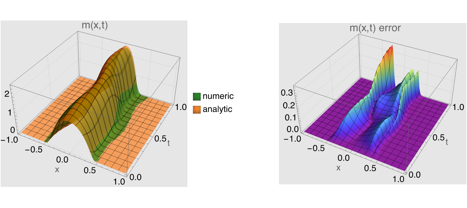
Fig. 3. Approximated and exact solutions for $m$ (left), and their absolute difference (right).

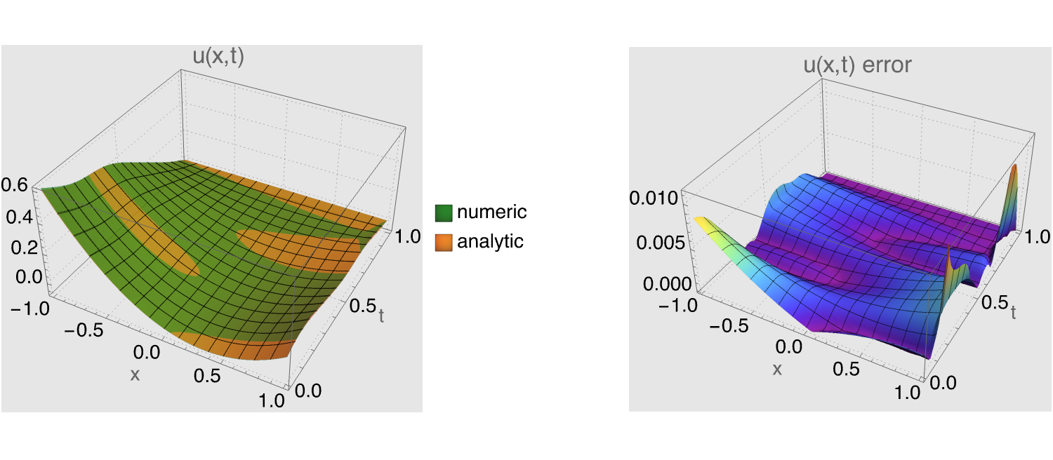
Fig. 4. Approximated and exact solutions for $u$ (left), and their absolute difference (right).

Table 1 presents $l^{\infty}$ error rates for various grid sizes, with all cases converging within 6 iterations for the tolerance parameter $\varepsilon=0.001$.

$\rho$	$h$	err. $\varpi$	err. $u$	err $m$
$1.0\cdot 10^{-1}$	$1.0\cdot 10^{-1}$	$2.4\cdot 10^{-2}$	$4.0\cdot 10^{-2}$	$7.2\cdot 10^{-1}$
$4.0\cdot 10^{-2}$	$4.0\cdot 10^{-2}$	$1.0\cdot 10^{-2}$	$1.6\cdot 10^{-2}$	$5.1\cdot 10^{-1}$
$2.0\cdot 10^{-2}$	$2.0\cdot 10^{-2}$	$5.3\cdot 10^{-3}$	$8.1\cdot 10^{-3}$	$3.6\cdot 10^{-1}$
$1.0\cdot 10^{-2}$	$1.0\cdot 10^{-2}$	$2.8\cdot 10^{-3}$	$3.8\cdot 10^{-3}$	$2.2\cdot 10^{-1}$

Table 1. Comparing errors on different grids, for tolerance parameter $\varepsilon=0.001$.

We also run our scheme with the same discretization parameters $\rho=0.05$ and $h=0.05$ and the same problem data as in [4], where authors used the variational method. Our scheme outperforms the variational method in accuracy for $\varpi$, $u$, and $m$, by approximately 10, 8, 1.5 times.

We also compared our scheme to the recurrent neural network method with the same problem data as given in [5]. With the discretization parameters $\rho=0.01$ and $h=0.01$, our scheme outperforms the recurrent neural network method in accuracy for $\varpi$, $u$, and $m$, by approximately and 15, 10, 3 times respectively.

These results demonstrate the efficacy of the Semi-Lagrangian scheme. We should stress, however, that the machine learning code was partially developed to address common noise problems that our method does not cover.

References

• [1] Y. Achdou, F. Camilli, and I. Capuzzo-Dolcetta. Mean field games: numerical methods for the planning problem. SIAM J. Control Optim., 50(1):77–109, 2012.
• [2] Y. Achdou and I. Capuzzo-Dolcetta. Mean field games: numerical methods. SIAM J. Numer. Anal., 48(3):1136–1162, 2010.
• [3] Y. Ashrafyan, T. Bakaryan, D. Gomes, and J. Gutierrez. A duality approach to a price formation mfg model. Minimax Theory and its Applications, 08(1):1–36, 2023.
• [4] Yuri Ashrafyan, Tigran Bakaryan, Diogo Gomes, and Julian Gutierrez. The potential method for price-formation models. 2022 IEEE 61st Conference on Decision and Control (CDC), pages 7565–7570, 2022.
• [5] Yuri Ashrafyan, Tigran Bakaryan, Diogo Gomes, and Julian Gutierrez. A variational approach for price formation models in one dimension. Communications in Mathematical Sciences, 22(1):227–255, 2024.
• [6] Martino Bardi and Italo Capuzzo-Dolcetta. Optimal Control and Viscosity Solutions of Hamilton-Jacobi-Bellman Equations. Birkhäuser Boston, MA, 1997.
• [7] Fabio Camilli and Francisco Silva. A semi-discrete approximation for a first order mean field game problem. Networks and Heterogeneous Media, 7(2):263–277, 2012.
• [8] E. Carlini and F. J. Silva. Semi-lagrangian schemes for mean field game models. pages 3115–3120, 2013.
• [9] E. Carlini and F. J. Silva. A fully discrete semi-lagrangian scheme for a first order mean field game problem. SIAM Journal on Numerical Analysis, 52(1):45–67, 2014.
• [10] P. G. Ciarlet and J.-L. Lions, editors. Handbook of numerical analysis. Vol. II. Handbook of Numerical Analysis, II. North-Holland, Amsterdam, 1991. Finite element methods. Part 1.
• [11] D. Gomes and J. Saúde. A Mean-Field Game Approach to Price Formation. Dyn. Games Appl., 11(1):29–53, 2021.
• [12] Diogo Gomes, Julian Gutierrez, and Mathieu Laurière. Machine learning architectures for price formation models. 88(23):1–14, 2023.
• [13] Diogo Gomes, Julian Gutierrez, and Mathieu Laurière. Machine learning architectures for price formation models with common noise. pages 4345–4350, 2023.
• [14] Diogo Gomes, Julian Gutierrez, and Ricardo Ribeiro. A mean field game price model with noise. Mathematics in Engineering, 3(4):1–14, 2021.
• [15] Diogo Gomes, Julian Gutierrez, and Ricardo Ribeiro. A random-supply mean field game price model. SIAM Journal on Financial Mathematics, 14(1):188–222, 2023.
• [16] M. Huang, P. E. Caines, and R. P. Malhamé. Large-population cost-coupled LQG problems with nonuniform agents: individual-mass behavior and decentralized $\epsilon$-Nash equilibria. IEEE Trans. Automat. Control, 52(9):1560–1571, 2007.
• [17] M. Huang, R. P. Malhamé, and P. E. Caines. Large population stochastic dynamic games: closed-loop McKean-Vlasov systems and the Nash certainty equivalence principle. Commun. Inf. Syst., 6(3):221–251, 2006.
• [18] J.-M. Lasry and P.-L. Lions. Jeux à champ moyen. I. Le cas stationnaire. C. R. Math. Acad. Sci. Paris, 343(9):619–625, 2006.
• [19] J.-M. Lasry and P.-L. Lions. Jeux à champ moyen. II. Horizon fini et contrôle optimal. C. R. Math. Acad. Sci. Paris, 343(10):679–684, 2006.
• [20] A. Quarteroni, R. Sacco, and F. Saleri. Numerical Mathematics (Second Ed.). Springer, Berlin, 2007.