Data Collaboration Analysis Over Matrix Manifolds

Abstract

The effectiveness of machine learning (ML) algorithms is deeply intertwined with the quality and diversity of their training datasets. Improved datasets, marked by superior quality, enhance the predictive accuracy and broaden the applicability of models across varied scenarios. Researchers often integrate data from multiple sources to mitigate biases and limitations of single-source datasets. However, this extensive data amalgamation raises significant ethical concerns, particularly regarding user privacy and the risk of unauthorized data disclosure. Various global legislative frameworks have been established to address these privacy issues. While crucial for safeguarding privacy, these regulations can complicate the practical deployment of ML technologies. Privacy-Preserving Machine Learning (PPML) addresses this challenge by safeguarding sensitive information, from health records to geolocation data, while enabling the secure use of this data in developing robust ML models. Within this realm, the Non-Readily Identifiable Data Collaboration (NRI-DC) framework emerges as an innovative approach, potentially resolving the ’data island’ issue among institutions through non-iterative communication and robust privacy protections. However, in its current state, the NRI-DC framework faces model performance instability due to theoretical unsteadiness in creating collaboration functions. This study establishes a rigorous theoretical foundation for these collaboration functions and introduces new formulations through optimization problems on matrix manifolds and efficient solutions. Empirical analyses demonstrate that the proposed approach, particularly the formulation over orthogonal matrix manifolds, significantly enhances performance, maintaining consistency and efficiency without compromising communication efficiency or privacy protections.

Keywords Privacy-Preserving Machine Learning  $\cdot$ Data Collaboration Analysis  $\cdot$ Orthogonal Procrustes Analysis  $\cdot$ Matrix Manifold Optimization

1 Introduction

The effectiveness of machine learning (ML) algorithms is deeply intertwined with the quality and diversity of their training datasets. Improved datasets, marked by superior quality, enhance the predictive accuracy and broaden the applicability of models across varied scenarios. Researchers often integrate data from multiple sources to mitigate biases and limitations of single-source datasets. However, this extensive data amalgamation raises significant ethical concerns, particularly regarding user privacy and the risk of unauthorized data disclosure.

The issue of data breaches further escalates these privacy concerns. Emerging research highlights an increasing wariness about the risks associated with the extensive collection and processing of personal data [50]. Additionally, ML models are vulnerable to several inference attacks that malicious entities could exploit. For example, membership inference attacks allow attackers to deduce whether data from specific individuals were used in training datasets [20]. Other significant threats include model inversion attacks [11], property inference attacks [13], and the risk of privacy violations through gradient sharing in distributed ML systems [63].

In response to these privacy issues, legislative frameworks such as the European General Data Protection Regulation (GDPR), the California Consumer Privacy Act (CCPA), and Japan’s amended Act on the Protection of Personal Information (APPI) have been implemented. These regulations, aimed at mitigating privacy challenges, establish stringent protocols for data management. While essential for privacy protection, they introduce complexities that may hinder the practical application of ML technologies. A notable complication is the emergence of ’data islands’ [33], which are isolated data segments within the same sector, often observed in fields like medicine, finance, and government. These segments typically contain limited data, which is insufficient for training comprehensive models representative of larger populations. A collaborative model training on a combined dataset from these islands would be ideal, but this is frequently unfeasible due to the regulations above. The field of Privacy-Preserving Machine Learning (PPML) is dedicated to overcoming this challenge, striving to protect sensitive information, ranging from health records to geolocation data, while facilitating the secure utilization of this data in the development of robust ML models.

Many PPML methodologies have emerged in recent years, driven by various factors: the implementation of established privacy measures, the development of innovative privacy-preserving techniques, the continuous evolution of ML models, and the enforcement of strict privacy regulations. In their comprehensive analysis, [59] provides an overview of current PPML methodologies and underscores the ongoing challenges and open problems in devising an optimal PPML solution:

1. "In terms of privacy protection, how can a PPML solution be assured of adequate privacy protection by the trust assumption and threat model settings? Generally, the privacy guarantee should be as robust as possible from the data owners’ standpoint."

2. "In terms of model accuracy, how can we ensure that the trained model in the PPML approach is as accurate as the model trained in the contrasted vanilla machine learning system without using any privacy-preserving settings?"

3. "In terms of model robustness and fairness, how can we add privacy-preserving capabilities without impairing the model’s robustness and fairness?"

4. "In terms of system performance, how can the PPML system communicate and compute as effectively as the vanilla machine learning system?"

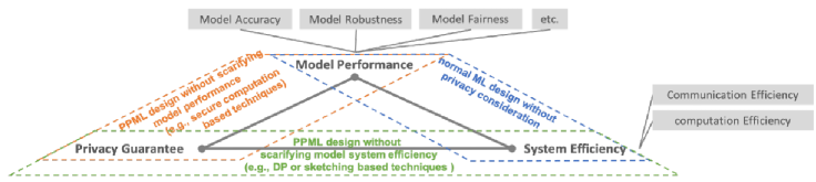
Figure 1: (Figure 4 in [59]) Trade-offs regarding the creation of PPML solutions.

The exploration of trade-offs in PPML, as depicted in Figure 1, highlights the intricate challenges in this field. These challenges primarily revolve around embedding adequate privacy protections into ML frameworks without compromising their core functions, namely model performance and system efficiency. A quintessential example of PPML methodologies stems from the domain of Secure Computation, a concept introduced by Andrew Yao in 1982 [61]. Secure computation aims to enable multiple parties to collaboratively compute an arbitrary function on their respective inputs while ensuring that only the function’s output is disclosed. This approach effectively maintains the confidentiality of the input data.

Several techniques in the field of secure computation stand out for their effectiveness and application. Among these are additive blinding methods [52, 7, 8], which obscure data elements by adding noise; garbled circuits [58, 3], facilitating secure function evaluation; and Homomorphic Encryption, which enables computations on encrypted data [42, 1]. Despite its over forty-year history, secure computation remains crucial in PPML advancements. Its ongoing relevance is demonstrated by its incorporation into contemporary applications [4, 14] and the development of complete PPML frameworks centered around it [51]. However, employing secure computation in PPML frameworks often introduces significant computation and communication overhead challenges. This challenge is particularly evident when handling large datasets or complex functions, even with the most recent implementations [62].

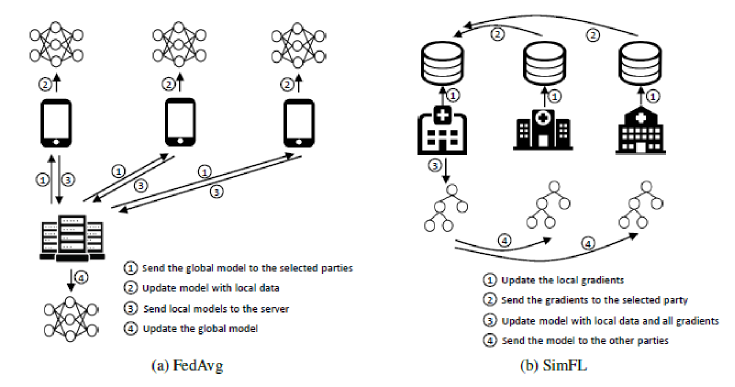
Figure 2: (Figure 2 in [33]) Federated Learning frameworks

Federated Learning (FL) [43, 31] stands out in PPML for its scalable, cross-device capabilities. Its core lies in collaboratively training a global model (or enhanced individual models) across multiple parties while keeping data localized, securely enhancing model performance over individual local models. A notable use case is the Google Keyboard [60], which uses FL for improved query suggestions without compromising privacy. A key FL algorithm is Federated Averaging (FedAvg) [43], where a central server distributes a model to clients for local improvements. The server aggregates these enhancements to refine the global model in an iterative process, as shown in Figure 2a.

SimFL, developed by Li et al. [31], offers a decentralized alternative instead of the centralized FedAvg model. Its key feature is the absence of a central server. Participants in SimFL independently update their local models using their data. Uniquely, instead of sending gradients to a central server after updates, they are shared with a randomly chosen participant. This participant integrates the received gradients into their model, which is then shared network-wide. This gradient exchange and model updating process is repeated for a set number of iterations, culminating in a jointly developed final model, as shown in Figure 2b.

One of the critical open problems in FL is addressing its inherent privacy challenges, as recent surveys and studies have pointed out [29, 41]. Once considered secure, the standard practice in FL of sharing gradients instead of raw data now reveals vulnerabilities to model inference attacks [11] by the potential of data leakage from gradients, as recent research indicates [63]. Moreover, FL is prone to poisoning attacks, where adversaries aim to degrade the model’s accuracy or manipulate its outputs [2]. In response, researchers are exploring hybrid approaches that meld FL with advanced secure computation techniques [55] or the incorporation of differential privacy [9]. While these methods enhance security, they also introduce trade-offs, such as increased computational demands and potential reductions in model performance [59]. These trade-offs exemplify the complexity of achieving robust privacy in FL without impairing the learning models’ efficiency and effectiveness.

Addressing non-identically and independently distributed (non-IID) data is also a significant challenge in FL, as highlighted in recent studies [32]. This challenge becomes particularly pronounced in cross-silo FL, which involves entities like banks, hospitals, and insurance companies, each with large, diverse datasets as ’data islands’. The inherent data heterogeneity in these environments renders assumptions of IID data distributions impractical. Consequently, standard FL techniques, especially FedAvg, face substantial challenges under these non-IID conditions [36]. Recent research has focused on developing advanced FL methods such as FedProx [35], SCAFFOLD [30], FedRobust [49], and FedDF [38], each tailored to manage non-IID data better. Despite these advancements, fully resolving the complexities associated with non-IID data in FL remains a formidable open problem in the field [34].

Specifically in cross-silo FL, another significant challenge is the necessity for iterative communication between institutions during each model training phase. This challenge is especially critical in sectors handling sensitive data, like healthcare, where medical institutions often operate within isolated networks. Traditional FL approaches rely heavily on iterative communication for model training, a bedrock issue in these environments.

In response, Data Collaboration (DC) analysis [24, 26, 23] has emerged as a notable alternative. Unlike typical FL frameworks that focus on model sharing, DC centralizes dimensionally reduced, secure intermediate representations of the raw data, eliminating the need for iterative model update exchanges. Although DC has limitations in cross-device contexts due to computational and scalability constraints, it effectively addresses other issues in cross-silo FL, especially in handling non-IID data distributions [44] and aligning misaligned feature spaces [45]. DC has been proven to have a double layer of privacy protection: the first layer for honest-but-curious participants and the second layer for malicious collusion between participants and man-in-the-middle attacks [22]. A recent variant, Non-Readily Identifiable DC (NRI-DC) analysis [25], further enhances privacy by ensuring that intermediate representations are not easily traceable to individuals or entities, aligning with global data privacy regulations.

The privacy-preserving aspect of DC analysis relies on sharing dimensionally reduced intermediate representations of raw data rather than the raw data itself. Each entity independently generates these representations using its unique, secret dimension reduction functions in this process, creating a robust privacy framework. While this technique is akin to data preprocessing approaches in PPML like differential privacy or k-anonymity [9, 54], it uniquely addresses the common challenge of reduced model utility. DC analysis overcomes this by ’aligning’ these intermediate representations into a unified collaborative representation with minimal distortion to their structures. This collaborative representation is created using a shared anchor dataset uniformly distributed to all entities. Each entity applies the same dimension reduction function to this anchor dataset as used on their raw data. With the anchor datasets being identical, a collaboration function is formulated to align the intermediate representations of the anchor data, aiming to minimize Frobenius norm error. When applied to the raw data’s intermediate representations, this collaboration function yields a collaborative representation suitable for training the global model. Chapter 2 and 3 will explore this methodology in greater detail.

This research is centered on developing an optimized collaboration function, a critical factor for the efficacy of the final ML model in DC frameworks. Constructing this function involves two primary steps: (i) defining a collaboration function optimization problem using the intermediate representations of the anchor data and (ii) resolving this problem efficiently. Present methods in the literature for crafting the collaboration function [24, 64] often exhibit theoretical gaps in their formulation phase, resulting in an unstable performance of ML models. This research endeavors to lay down a theoretically robust framework for the collaboration function’s formulation and to introduce a potent solution approach. The guiding research question is:

Can we develop a collaboration function formularization that is both robust and efficient, such that it not only enhances the performance and stability of the model but also adheres to the constraints of computational efficiency without undermining non-iterative communication and privacy guarantees of the DC framework?

To realize this objective, we propose optimization formulations over matrix manifolds, focusing on maximizing structure retainment of the intermediate representations. We achieve efficient problem-solving by utilizing established Procrustean analysis methods [15] and cutting-edge Riemannian optimization strategies [21, 6]. Our approaches are expected to improve the functionality and stability of the collaboration function significantly.

The key contributions of this research are outlined as follows:

1. Development of a novel and theoretically grounded formulation for the collaboration function in the Non-Readily Identifiable Data Collaboration (NRI-DC) framework.

2. Introduction of a practical solution approach for this formulation using established Procrustean analysis methods and Riemannian optimization algorithms.

3. Empirical evaluation using public datasets and various machine learning models, demonstrating the stable and superior performance of our proposed methods compared to existing approaches within the NRI-DC framework.

The organization of this research is as follows:

Section 2 provides an in-depth review of the Non-Readily Identifiable Data Collaboration (NRI-DC) framework. This section details the privacy-preserving mechanisms integral to the NRI-DC framework. In Section 3, we delve into the detailed process of formulating the collaboration function. We start by examining existing methodologies and then introduce our novel approaches, which include formulating optimization problems over matrix manifolds. We aim to establish that our method provides a more theoretically robust and valid approach to optimizing the collaboration functions, focusing on maximizing structure retainment of the intermediate representations. Section 4 presents empirical studies to assess the effectiveness of our proposed method. Comparing it with current methods using various public datasets and ML models, we aim to empirically show that our approach yields stable results and often excels in performance compared to traditional methods while maintaining computational efficiency. Section 5 concludes the research. This final section summarizes the main findings, discusses their implications, and offers perspectives on future research avenues.

2 Non-Readily Identifiable Data Collaboration Framework

This section examines the Non-Readily Identifiable Data Collaboration (NRI-DC) framework by Imakura et al. [25]. It begins with defining data identifiability and emphasizing its relevance to international data privacy regulations. Subsequently, we delve into the mechanics of the NRI-DC algorithm. We conclude the section with an analysis of the algorithm’s inherent privacy-preserving mechanisms.

2.1 Definition of Identifiability

In data analysis involving personal information, adherence to various privacy laws, professional responsibilities, and custodial obligations is imperative. This adherence becomes particularly critical when such analyses are outsourced, compelling the analytical organization to conform to the exact stringent requirements. The scope of these obligations extends beyond data that is directly identifiable. It also encompasses data that, although not directly linked to personal identifiers, can be amalgamated with other information to identify individuals indirectly. Key global legislations define personal information as follows:

• GDPR (EU): Article 4(1) - "Personal data" means any information relating to an identified or identifiable natural person (’data subject’); an identifiable natural person is one who can be identified, directly or indirectly.

• CCPA (USA): Section 1798.140(o) - "Personal information" means information that identifies, relates to, describes, is capable of being associated with, or could reasonably be linked, directly or indirectly, with a particular consumer or household.

• Amended APPI (Japan): Article 2 - "Personal information" in this Act means that information relating to a living individual . . . (including those which can be readily collated with other information and thereby identify a specific individual).

Given these legislations, the identifiability of shared information emerges as a pivotal element in privacy-preserving analysis since readily identifiable data are subject to the same stringent regulations as personal information. Therefore, for practical privacy preservation in analyses involving multiple datasets that contain personal information, it is imperative to ensure that the shared data are non-readily identifiable from the original data. This approach forms the bedrock of maintaining confidentiality and complying with global data protection standards. [25] provides a mathematical definition for the identifiability of data that follows these standards:

Definition 2.1.

(Definition 1. in [25]) Definition of Identifiability
Let $x^{p}_{i}$ and $x^{np}_{i}$ represent paired data for the $i$-th individual from a set of $n$ people, including and excluding personal information that can directly identify an individual, respectively. Define $\chi^{p}=\{x^{p}_{1},x^{p}_{2},\ldots,x^{p}_{n}\}$ as the dataset of personal information and $\chi^{np}=\{x^{np}_{1},x^{np}_{2},\ldots,x^{np}_{n}\}$ as the dataset of non-personal information, for the same set of $n$ individuals.
The non-personal dataset $\chi^{np}$ is considered "readily identifiable" from the personal dataset $\chi^{p}$, if and only if a third party holds a key (or a precise approximation) that can correctly associate $x^{np}\in\chi^{np}$ with $x^{p}\in\chi^{p}$, or if the data owner can independently derive such a key (or a precise approximation).

Common unique identifiers and specific features can be used as keys to collating data. Furthermore, precise approximations of these features can also act as keys, enabling the correct association of corresponding data elements. [25] also establishes the following property on readily identifiable data:

Proposition 2.2.

(Proposition 1. in [25])
If either of the following conditions holds, we can say $\chi^{np}$ is readily identifiable from $\chi^{p}$.

• The data holder of $\chi^{p}$ possesses or can independently generate a function $v$ (or a precise approximation) such that $x^{np}_{i}=v(x^{p}_{i})$.

• The data holder of $\chi^{np}$ possesses or can independently generate a function $w$ (or a precise approximation) such that $x^{p}_{i}=w(x^{np}_{i})$.

Proof. In the case where the data holder of $\chi^{p}$ holds the function $v$ such that $x^{np}_{i}=v(x^{p}_{i})$ or can generate the function on their own, they can obtain pairs of $(x^{p}_{i},x^{np}_{i})$ corresponding to any $x^{p}_{i}\in\chi^{p}$ using the function $v$. Therefore, using $x^{np}_{i}$ as a key, for non-personal information $x^{np}\in\chi^{np}$, the corresponding personal information $x^{p}\in\chi^{p}$ can be collated accurately.

In the same manner, in the case where the data holder of $\chi^{np}$ holds the function $w$ such that $x^{p}_{i}=w(x^{np}_{i})$ or can generate the function by their own, they can obtain pairs of $(x^{p}_{i},x^{np}_{i})$ corresponding to any $x^{np}_{i}\in\chi^{np}$ using the function $w$. Therefore, using $x^{p}_{i}$ as a key, for non-personal information $x^{np}\in\chi^{np}$, the corresponding personal information $x^{p}\in\chi^{p}$ can be collated accurately. ∎

A counter-intuitive example of Proposition 2.2 is the case of datasets encrypted for homomorphic encryption computation. Such datasets are deemed readily identifiable despite the encryption because the original data owner possesses encryption and decryption capabilities. Indeed, privacy-preserving machine learning frameworks that ensure the shared datasets are non-readily identifiable from the raw data have a significant advantage in social implementation regarding the current global legislation.

2.2 NRI-DC Algorithm

Input: For worker-side: $X_{i}\in\mathbb{R}^{n_{i}\times m}$, $Y_{i}\in\mathbb{R}^{n_{i}\times l}$, and $X_{i}^{\mathrm{test}}\in\mathbb{R}^{n_{i}^{\mathrm{test}}\times m}$ individually.

Output: For worker-side: $Y_{i}^{\mathrm{pred}}$ ($i=1,2,\ldots,c$).

         Worker-side ($i=1,2,\ldots,c$)

  ——————————————————————————–

1. Generate $X^{\mathrm{anc}}\in\mathbb{R}^{r\times m}$ and share to all workers.

2. Generate random permutation matrix $P_{i}\in\mathbb{R}^{n_{i}\times n_{i}}$

that cannot be reconstructed.

Generate random matrix $E_{i}\in\mathbb{R}^{n_{i}\times m}$ that cannot be

reconstructed and choose perturbation parameter $\delta_{i}$.

Generate PCA linear dimension reduction function

$F_{i}\in\mathbb{R}^{m\times\tilde{m}}$ based on $X_{i}+\delta_{i}E_{i}$.

Compute $\tilde{X^{\prime}_{i}}=P_{i}X_{i}F^{\prime}_{i}$, $\tilde{X}^{\mathrm{anc}}_{i}=X^{\mathrm{anc}}F^{\prime}_{i}$, and $\tilde{Y_{i}}=P_{i}Y_{i}$. 6. Erase $F^{\prime}_{i}$ and $P_{i}$. 7. Share $\tilde{X^{\prime}_{i}}$, $\tilde{X}^{\mathrm{anc}}_{i}$, and $\tilde{Y^{\prime}_{i}}$ to master and erase them. Master-side

              ————————————————————–

1. $\searrow$      Obtain $\tilde{X^{\prime}_{i}}$, $\tilde{X}^{\mathrm{anc}}_{i}$, and $\tilde{Y^{\prime}_{i}}$ for all $i$.

2. ​Compute $G_{i}\in\mathbb{R}^{\tilde{m}\times\tilde{m}}$ from $\tilde{X}^{\mathrm{anc}}$ for all $i$.

3. ​Compute ${\hat{X}}_{i}=\tilde{X^{\prime}_{i}}G_{i}$ for all $i$, and set ${\hat{X}}^{\prime},Y^{\prime}$.

4. ​Analyze ${\hat{X}}^{\prime}$ to obtain $h$ such that $Y^{\prime}\approx h({\hat{X}}^{\prime})$.

5. ​Compute $Y^{\mathrm{anc}}_{i}=h({\hat{X}^{\mathrm{anc}}}_{i})$.

6. $\swarrow$      Return $Y^{\mathrm{anc}}_{i}$ to each worker.

         Worker-side ($i=1,2,\ldots,c$)

  ——————————————————————————–

1. Obtain $Y^{\mathrm{anc}}_{i}$.

2. Analyze $X^{\mathrm{anc}}$ to obtain $t_{i}$ such that $Y^{\mathrm{anc}}_{i}\approx t_{i}(X^{\mathrm{anc}})$.

3. Compute $Y_{i}^{\mathrm{pred}}=t_{i}(X_{i}^{\mathrm{test}})$.

Algorithm 1 (Algorithm 2 in [25]) Overview of the NRI-DC algorithm

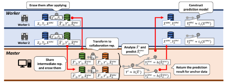
Figure 3: (Figure 2 in [25]) Overview of the non-readily identifiable DC framework

This section reviews the NRI-DC framework proposed by Imakura et al. [25]. This framework focuses on supervised machine learning for classification tasks for multiple entities, each with strict privacy protocols. The goal is to construct a prediction or classification model from labeled training datasets.

Consider a dataset $X^{\mathrm{all}}$ consisting of $n$ training samples with $m$ features each and a corresponding label set $Y^{\mathrm{all}}$ with $l$ labels. Specifically, $X^{\mathrm{all}}=[x_{1},x_{2},\ldots,x_{n}]^{\top}\in\mathbb{R}^{n\times m}$ and $Y^{\mathrm{all}}=[y_{1},y_{2},\ldots,y_{n}]^{\top}\in\mathbb{R}^{n\times l}$ represent the training data and labels, respectively. For privacy-preserving analysis across multiple entities, we examine a scenario where the dataset is horizontally partitioned across $c$ different entities. This partitioning is formalized as:

$$X^{\mathrm{all}}=\begin{bmatrix}X_{1}\\ X_{2}\\ \vdots\\ X_{c}\end{bmatrix},\quad Y^{\mathrm{all}}=\begin{bmatrix}Y_{1}\\ Y_{2}\\ \vdots\\ Y_{c}\end{bmatrix},$$

where each entity $i$ possesses a subset of the data, $X_{i}\in\mathbb{R}^{n_{i}\times m}$ and labels $Y_{i}\in\mathbb{R}^{n_{i}\times l}$, with the total number of samples given by $n=\sum_{i=1}^{c}n_{i}$. Note that the NRI-DC framework can be applied to more sophisticated distributions such as partially common features [45] and horizontally or (and) vertically partitioned data [26].

The framework operates with two roles: worker and master. Workers have their private dataset and corresponding ground truth, $X_{i}$ and $Y_{i}$, and aim to improve their local classification model by using insights from other workers’ data without sharing their own. The master facilitates this process.

Initially, each worker creates a common anchor dataset, denoted as $X^{\mathrm{anc}}\in\mathbb{R}^{r\times m}$. This dataset comprises either public data or synthetically generated dummy data. Generally, a random matrix is effective for this purpose [24, 26, 27]. Importantly, this anchor data remains concealed from the master.

Each worker then creates a row-wise dimension reduction function $f^{\prime}_{i}:\mathbb{R}^{p\times m}\rightarrow\mathbb{R}^{p\times\tilde{m}}$ (where $p$ denotes an arbitrary number of rows) that transforms raw data into the secure, non-readily identifiable intermediate representations. For simplicity, we choose a linear dimension reduction matrix $F^{\prime}_{i}\in\mathbb{R}^{m\times\tilde{m}}$ for $f^{\prime}_{i}$, specifically a Principal Component Analysis (PCA) [12] transformation matrix based on the raw data plus random permutation $X_{i}+\delta_{i}E_{i}$. Here, $E_{i}\in\mathbb{R}^{n_{i}\times m}$ is a random matrix whose entries are uniform random numbers in $[-1,1]$ and $\delta_{i}\in(0,1)$ are perturbation parameters chosen by each worker. Additionally, workers create a random permutation matrix $P_{i}\in\mathbb{R}^{n_{i}\times n_{i}}$ and use these components to calculate the intermediate representations:

$$\tilde{X^{\prime}_{i}}=P_{i}X_{i}F^{\prime}_{i},\quad\tilde{X}^{\mathrm{anc}}_{i}=X^{\mathrm{anc}}F^{\prime}_{i},\quad\tilde{Y^{\prime}_{i}}=P_{i}Y_{i}.$$ (1)

Workers then share the intermediate representations $\tilde{X^{\prime}_{i}},\tilde{X}^{\mathrm{anc}}_{i}$, and $\tilde{Y^{\prime}_{i}}$ with the master. To prevent identification of the raw data from these representations, each worker deletes $F^{\prime}_{i}$ and $P_{i}$ after use. In classification tasks, $P_{i}$ cannot be inferred from $\tilde{Y^{\prime}_{i}}$ and $Y_{i}$ due to the non-uniqueness of their rows. The exact $F^{\prime}_{i}$ cannot be regenerated because it is created based on the raw data plus a random permutation $X_{i}+\delta_{i}E_{i}$ that cannot be reconstructed.

On the master’s side, the task is to align the workers’ intermediate representations $\tilde{X^{\prime}_{i}}$ into a common, lower-dimensional space with a similar orientation to make them comparable. This is achieved using linear mapping functions, denoted as $G_{i}\in\mathbb{R}^{\tilde{m}\times\tilde{m}}$. Linear mappings are chosen because of their simplicity, and non-linear mappings are an essential topic for future exploration. However, numerical experiment results in contemporary research show that linear mappings perform adequately [44, 23]. $G_{i}$ are created leveraging that the $\tilde{X}^{\mathrm{anc}}_{i}$ were identical across all workers before being transformed by PCA. The specifics of creating $G_{i}$ are detailed in Chapter 3 since it is the crux of this research. In this chapter, we assume $G_{i}$ has been effectively established, allowing us to focus on the framework’s overview and privacy implications.

Once we have $G_{i}$, we compute the collaborative representations as follows:

$${\hat{X}}^{\prime}=[(\tilde{X^{\prime}_{1}}G_{1})^{\top},(\tilde{X^{\prime}_{2}}G_{2})^{\top},...,(\tilde{X^{\prime}_{c}}G_{c})^{\top}]^{\top},\quad Y^{\prime}=[\tilde{Y^{\prime}_{1}}^{\top},\tilde{Y^{\prime}_{2}}^{\top},...,\tilde{Y^{\prime}_{c}}^{\top}]^{\top}.$$ (2)

We analyze ${\hat{X}}^{\prime}$ and $Y^{\prime}$ to create a supervised classification model $h$:

$$Y^{\prime}\approx h({\hat{X}}^{\prime}).$$

Using the model $h$, we leverage prediction results $Y^{\mathrm{anc}}_{i}$ of the anchor data $X^{\mathrm{anc}}$:

$$Y^{\mathrm{anc}}_{i}=h({\hat{X}^{\mathrm{anc}}}_{i}),\quad{\hat{X}^{\mathrm{anc}}}_{i}=\tilde{X}^{\mathrm{anc}}_{i}G_{i}\in\mathbb{R}^{r\times\tilde{m}}.$$

The prediction results $Y^{\mathrm{anc}}_{i}$ obtained from $X^{\mathrm{anc}}$ are sent back to the $i$th worker. Subsequently, each worker constructs the prediction model $t_{i}$ using supervised machine learning or deep learning techniques based on the data $X^{\mathrm{anc}}$ and the corresponding predictions $Y^{\mathrm{anc}}_{i}$:

$$Y^{\mathrm{anc}}_{i}\approx t_{i}(X^{\mathrm{anc}}).$$

For the prediction phase, the prediction result $Y_{i}^{\mathrm{pred}}$ of $X_{i}^{\mathrm{test}}$ is obtained by

$$Y_{i}^{\mathrm{pred}}=t_{i}(X_{i}^{\mathrm{test}}).$$

The overview of the NRI-DC framework is summarized in Algorithm 1 and Figure 3. Note that the framework only requires three cross-institutional communications, namely Steps 1, 7, and 13 in Algorithm 1.

2.3 Discussions on Privacy

This section reviews the privacy implications and limitations of the NRI-DC framework analyzed in [22, 25]. Here, we assume that the workers and the master are honest-but-curious, meaning they adhere to the framework’s procedures but may attempt to glean private data $X_{i}$ using any accessible vulnerabilities. [22] claims the framework incorporates dual-layer privacy protection. The first layer safeguards against breaches from individual users and the master. The second layer addresses potential external man-in-the-middle attacks and collusion between the workers and the master.

Privacy against the honest-but-curious master

Theorem 2.3.

(Theorem 2 in [22]) The master cannot infer the users’ private datasets $X_{i}$ when adhering strictly to the procedures of the NRI-DC framework and does not collide with any of the users.

Proof. Under the algorithm’s framework, the master gains access to $\tilde{X^{\prime}_{i}}$ and $\tilde{X}^{\mathrm{anc}}_{i}$, but not to $F^{\prime}_{i}$, or $X^{\mathrm{anc}}$. The master only encounters the outputs $\tilde{X^{\prime}_{i}}$ and $\tilde{X}^{\mathrm{anc}}_{i}$ of the dimension reduction process $F^{\prime}_{i}$, which offers no information about $X_{i}$ and $X^{\mathrm{anc}}$. Since $F^{\prime}_{i}$ is a dimension reduction function, it does not provide any features that could link $X_{i}$ and $\tilde{X^{\prime}_{i}}$. Furthermore, $F^{\prime}_{i}$ is a PCA transformation matrix tailored to the private dataset $X_{i}$, and even if the exact method of constructing $F^{\prime}_{i}$ is known, the matrix $F^{\prime}_{i}$ itself remains undetermined. Thus, if the master follows the NRI-DC framework’s procedures and does not collide with any users, it cannot access the private dataset $X_{i}$. ∎

Privacy against the honest-but-curious workers

Theorem 2.4.

(Theorem 3 in [22]) Any user $i$ cannot infer the other users’ private datasets $X_{j}(i\neq j)$ when adhering strictly to the procedures of the NRI-DC framework and does not collide with the master.

Proof. Under the algorithm’s framework, the user $i$ gains access to $X^{\mathrm{anc}}$, but not to $\tilde{X^{\prime}_{j}},\tilde{X}^{\mathrm{anc}}_{j},F^{\prime}_{j}$. User $i$ only encounters the input $X^{\mathrm{anc}}$ of any other user $j$’s dimension reduction process $F^{\prime}_{j}$, which obviously offers no information about $X_{j},\tilde{X^{\prime}_{j}}$ and $\tilde{X}^{\mathrm{anc}}_{j}$. Since we can use a random matrix for $X^{\mathrm{anc}}$, no information can be inferred about $X_{j}$ from $X^{\mathrm{anc}}$. ∎

Privacy against the collusion between user and master

When user $i$ and the master collude, they gain access to $X^{\mathrm{anc}}$, $\tilde{X}^{\mathrm{anc}}_{j}$, and $\tilde{X^{\prime}_{j}}$. In this scenario, they possess both the input $X^{\mathrm{anc}}$ and the output $\tilde{X}^{\mathrm{anc}}_{j}$ of the dimension reduction function $F^{\prime}_{j}$ used by the target user $j$. The risk here is the potential reconstruction of the dimension reduction $F^{\prime}_{j}$ to infer $X_{j}$ from $\tilde{X^{\prime}_{j}}$. Although $F_{j}$ is a dimension reduction function and does not allow for an exact inverse, the Moore-Penrose pseudoinverse ${F^{\prime}}_{j}^{\dagger}$ can serve as a reasonable approximation, assuming the raw datasets are standardized. Reference [46] provides a formal definition of privacy in the context of dimension reduction, termed $\varepsilon$-DR Privacy:

Definition 2.5.

($\varepsilon$-DR Privacy) (Definition 1 in [46]) A Dimension Reduction Function $F(\cdot)$ satisfies $\varepsilon$-DR Privacy if for each i.i.d. $m$-dimension input sample $x$ drawn from the same distribution $D$, and for a certain distance measure $\text{dist}(\cdot,\cdot)$, we have

$$\mathbb{E}[\text{dist}(x,x^{\prime})]\geq\varepsilon,$$

where $\mathbb{E}[\cdot]$ is the expectation, $\varepsilon\geq 0$, $\tilde{x}=F(x)$, $x^{\prime}=R(\tilde{x})$, and $R(\cdot)$ is the Reconstruction Function.

[22] examines the privacy assurances related to $\epsilon$-DR Privacy within the DC framework. Below, we summarize their key points and define $\epsilon$-DR Privacy for the DC framework:

Definition 2.6.

($\varepsilon$-DR Privacy for DC) For a given $\varepsilon\geq 0$, a linear dimension reduction function $F^{\prime}\in\mathbb{R}^{m\times\tilde{m}}$ satisfies $\varepsilon$-DR Privacy regarding an $m$-feature data sample set $\chi=\{x_{1},x_{2},...,x_{n}\}$, if we have

$$\min_{x\in\chi}\frac{||x-xF^{\prime}{F^{\prime}}^{\dagger}||_{2}}{||x||_{2}}\geq\varepsilon,$$ (3)

where ${F^{\prime}}^{\dagger}$ denotes the Moore-Penrose pseudoinverse of $F^{\prime}$.

Regarding this definition, [22] introduces a down-sampling technique that eliminates samples that do not satisfy (3) for a pre-determined $\varepsilon$. Their numerical experiments show that despite the down-sampling, the effect on the resulting model’s recognition performance is insignificant.

Privacy against external attacks

When utilizing secure data transmission protocols like Transport Layer Security (TLS), where information is encrypted using the private keys of the involved parties, the collaborative data analysis framework safeguards the private dataset $X_{i}$ from potential man-in-the-middle attacks. It is important to note that this approach relies on encrypted communication for non-private data rather than secure multi-party computation techniques.

However, without such secure data transmission protocols, the scenario resembles a situation where workers and the master collude. In this case, man-in-the-middle attackers could deduce $F^{\prime}_{i}$ using $X^{\mathrm{anc}}$ and $\tilde{X}^{\mathrm{anc}}_{i}$, leading to the potential inference of $X_{i}$. This risk resembles the threat posed when workers and the master collude.

Identifiability of the intermediate representations

The identifiability of the intermediate representations $\tilde{X^{\prime}_{i}}$ are analyzed through the following considerations:

• There are no common features linking $X_{i}$ and $\tilde{X^{\prime}_{i}}$ due to the nature of the function $F^{\prime}_{i}$.

• The absence of common sample IDs between $X_{i}$ and $\tilde{X^{\prime}_{i}}$ is ensured by using a random permutation $P_{i}$ that is irreproducible.

• The function $F^{\prime}_{i}$ is effectively non-existent for analysis purposes, as it cannot be reconstructed as it is based on raw data plus some random permutation $X_{i}+\delta_{i}E_{i}$ and is deleted prior to the sharing of $\tilde{X^{\prime}_{i}}$. It can only be reconstructed through the collusion of the $i$th worker and the master by examining $\tilde{X}^{\mathrm{anc}}_{i}$ and $X^{\mathrm{anc}}$.

Therefore, based on Definition 2.1 and Proposition 2.2, the intermediate representations $\tilde{X^{\prime}_{i}}$ are non-readily identifiable from the original data $X_{i}$, provided that both $\tilde{X}^{\mathrm{anc}}_{i}$ and $X^{\mathrm{anc}}$ are not accessible to any single entity. Even in extreme scenarios where we assume collusion between the workers and the master and both $\tilde{X}^{\mathrm{anc}}_{i}$ and $X^{\mathrm{anc}}$ are exposed, no inverse function ${F^{\prime}}_{i}^{-1}$ exists to retrieve $X_{i}$ from $\tilde{X^{\prime}_{i}}$, given the dimension reduction property of $F^{\prime}_{i}$. The accuracy of the approximation ${F^{\prime}}_{i}^{\dagger}$ can be reduced by down-sampling as required by $\varepsilon$-DR Privacy (2.6), with minimal impact on the utility of the model.

3 The Collaboration Function

This section focuses on the construction of collaboration functions $G_{i}$ using the intermediate representations $\tilde{X}^{anc}_{i}$ from the anchor dataset, as outlined in Step 9 of Algorithm 1. Subsection 3.1 lays out the necessary conditions for developing the collaborative function, setting the framework for the data collaboration problem, and emphasizing the importance of preserving the structure in the intermediate representations. In Subsection 3.2, we review current methodologies for formulating $G_{i}$. Subsection 3.3 introduces our novel approaches for constructing $G_{i}$, framing the concept of structure retention in intermediate representations as optimization problems on matrix manifolds. Efficient resolution techniques are discussed, employing established Procrustean analysis methods and advanced Riemannian optimization strategies.

3.1 The Data Collaboration Problem

As briefly discussed in Section 2.2, the intermediate representations $\tilde{X^{\prime}_{i}}=P_{i}X_{i}F^{\prime}_{i}\in\mathbb{R}^{n_{i}\times\tilde{m}}$ for each worker are created using a PCA transformation matrix $F^{\prime}_{i}\in\mathbb{R}^{m\times\tilde{m}}$ learned on each worker’s raw data plus some random matrix $X_{i}+\delta E_{i}\in\mathbb{R}^{n_{i}\times m}$ and a random perturbation $P_{i}\in\mathbb{R}^{n_{i}\times n_{i}}$ (1). These intermediate representations are generally not comparable across different $i\in\{1,2,...,c\}=[c]$ because intuitively the features generally correspond to different principal components derived from different datasets $X_{i}+\delta E_{i}$.

More formally, since the $\tilde{m}$-dimensional feature space spanned by the orthonormal column vectors of $F^{\prime}_{i}$ generally differ in terms of its dimensionality and its orientation in the higher $m$-dimensional space, it is meaningless to compare the intermediate representations $\tilde{X^{\prime}_{i}}$ from different workers.

To overcome this difficulty, the master finds the optimal linear collaboration functions $G_{i}\in\mathbb{R}^{\tilde{m}\times\tilde{m}}$, such that they map $\tilde{X^{\prime}_{i}}$ to a lower $\tilde{m}$-dimensional space which is most similar in terms of their orientation in the higher dimensional space. In other words, the master aims to align the features of $\tilde{X^{\prime}_{i}}$ to ensure comparability across different workers. This can be formulated as $F^{\prime}_{i}G_{i}=F^{\prime}_{j}G_{j}\quad(\forall i,j\in[c])$, but such $G_{i}$ may not exist depending on $F^{\prime}_{i}$ and the choice of $\tilde{m}$. We attempt to approximate this relationship by finding $G_{i},G_{j}$ for any pair of workers $i,j\in[c]$ such that, given an arbitrary $m$-dimensional data sample $x$, $F^{\prime}_{i}G_{i}$ and $F^{\prime}_{j}G_{j}$ will map $x$ to approximately the same point on the lower $\tilde{m}$ dimensional space:

$$x^{\top}F^{\prime}_{i}G_{i}\approx x^{\top}F^{\prime}_{j}G_{j}.$$

Here, we also need to constrain $G_{i}$ such that it minimizes distortion of the relationships in $\tilde{X^{\prime}_{i}}$. Formally, for an arbitrary pair of $m$-dimensional data samples $x,y$ and an arbitrary relationship $D(x,y)$ between them:

$$D(x,y)\approx D(x^{\top}F^{\prime}_{i}G_{i},y^{\top}F^{\prime}_{i}G_{i}).$$

We summarize the necessary conditions for optimal linear collaboration functions:

Conditions for optimal linear collaboration functions
Given an arbitrary pair of workers $i,j\in[c]$ with their corresponding PCA transformation matrices $F^{\prime}_{i}\in\mathbb{R}^{m\times\tilde{m}},F^{\prime}_{j}\in\mathbb{R}^{m\times\tilde{m}}$ and an arbitrary pair of $m$-dimensional data samples $x,y\in\mathbb{R}^{m}$, the corresponding linear collaboration functions $G_{i}\in\mathbb{R}^{\tilde{m}\times\tilde{m}},G_{j}\in\mathbb{R}^{\tilde{m}\times\tilde{m}}$ are optimal only if the following conditions hold:

1. $x^{\top}F^{\prime}_{i}G_{i}\approx x^{\top}F^{\prime}_{j}G_{j}$,

2. $D(x,y)\approx D(x^{\top}F^{\prime}_{i}G_{i},y^{\top}F^{\prime}_{i}G_{i})$,

where $D(\cdot,\cdot)$ denotes an arbitrary relationship between two data samples.

Since the PCA transformation matrices $F^{\prime}_{i}$ are not revealed to the master, the intermediate representations of the cross-worker-equivalent anchor dataset $\tilde{X}^{\mathrm{anc}}_{i}\in\mathbb{R}^{r\times\tilde{m}}$ are used instead. These conditions can be transformed using $\tilde{X}^{\mathrm{anc}}_{i}$ as follows:

Problem 3.1.

(The Data Collaboration Problem)
Given an arbitrary pair of workers $i,j\in[c]$ with their corresponding intermediate representations of the anchor data matrices $\tilde{X}^{\mathrm{anc}}_{i}\in\mathbb{R}^{r\times\tilde{m}},\tilde{X}^{\mathrm{anc}}_{j}\in\mathbb{R}^{r\times\tilde{m}}$, the corresponding linear collaboration functions $G_{i}\in\mathbb{R}^{\tilde{m}\times\tilde{m}},G_{j}\in\mathbb{R}^{\tilde{m}\times\tilde{m}}$ are optimal only if the following conditions hold:

1. $\tilde{X}^{\mathrm{anc}}_{i}G_{i}\approx\tilde{X}^{\mathrm{anc}}_{j}G_{j}$,

2. $D^{\prime}(\tilde{X}^{\mathrm{anc}}_{i})\approx D^{\prime}(\tilde{X}^{\mathrm{anc}}_{i}G_{i})$,

where $D^{\prime}(X)$ denotes an arbitrary relationship between data samples of matrix X.

We denote this problem the Data Collaboration Problem, and we aim to find a theoretically robust mathematical formulation and an efficient approach to find the best-performing collaboration functions $G_{i}$.

3.2 Existing Methods

3.2.1 Least-Square Method

Imakura et al. (2020) [24] introduced a practical method for computing the collaboration function. They formulated equation (i) in (3.1) as the minimization problem of the sum of squared Frobenius norm distance between all pairs of $\tilde{X}^{\mathrm{anc}}_{i}G_{i},\tilde{X}^{\mathrm{anc}}_{j}G_{j}$:

$$\min_{G_{i}(i\in[c])}\sum_{i,j}||\tilde{X}^{\mathrm{anc}}_{i}G_{i}-\tilde{X}^{\mathrm{anc}}_{j}G_{j}||_{\mathrm{F}}^{2}.$$ (4)

Since $G_{i}$ has a trivial solution $G_{i}=\mathbf{0}$ in this formulation, they chose an objective matrix $Z=U_{1}$ such that:

$$[\tilde{X}^{\mathrm{anc}}_{1},\ldots,\tilde{X}^{\mathrm{anc}}_{c}]=[U_{1},U_{2}]\begin{bmatrix}\Sigma_{1}&\\ &\Sigma_{2}\\ \end{bmatrix}\begin{bmatrix}V_{1}^{\top}\\ V_{2}^{\top}\\ \end{bmatrix}\approx U_{1}\Sigma_{1}V_{1}^{\top}.$$ (5)

Where $U_{1}$ denotes the first $\tilde{m}$ columns of the left matrix of the singular value decomposition (SVD) of $[\tilde{X}^{\mathrm{anc}}_{1},\ldots,\tilde{X}^{\mathrm{anc}}_{c}]$ corresponding to the larger $\tilde{m}$ singular values. Using $Z=U_{1}$ as the objective matrix, they transform (4) to the following least square formulation:

$$\min_{G_{i}(i\in[c])}\sum_{i}||\tilde{X}^{\mathrm{anc}}_{i}G_{i}-Z||_{\mathrm{F}}^{2}.$$ (6)

They provide an approximate analytical solution to this formulation:

$$G*_{i}=(\tilde{X}^{\mathrm{anc}}_{i})^{\dagger}Z.$$ (7)

3.2.2 Generalized Eigenvalue Problem Method

Kawakami noted in his master’s thesis [64] that the least-square approach for determining $G_{i}$ (6) may be overly restrictive. He pointed out that selecting an objective matrix $Z$ constrained to have orthonormal columns (5), limits the search space for $G_{i}$.

His method first decomposes $G_{i}$ into column vectors

$$G_{i}=[g_{i1},\dots,g_{ik},\dots,g_{i\tilde{m}}],$$ (8)

and adds 2-norm constraints to equation (4) to handle the trivial solutions:

$$\min_{g_{ik}} \sum_{i,j}||\tilde{X}^{\mathrm{anc}}_{i}g_{ik}-\tilde{X}^{\mathrm{anc}}_{j}g_{jk}||_{2}^{2},$$ (9)

s.t. $$\sum_{i=1}^{c}||\tilde{X}^{\mathrm{anc}}_{i}g_{ik}||_{2}^{2}-1=0.$$

By defining matrices $A$ and $B$, vectors $v_{k}$:

$$A=\begin{pmatrix}2(c-1)\tilde{X}^{\mathrm{anc}\top}_{1}\tilde{X}^{\mathrm{anc}}_{1}&-2\tilde{X}^{\mathrm{anc}\top}_{1}\tilde{X}^{\mathrm{anc}}_{2}&\cdots&-2\tilde{X}^{\mathrm{anc}\top}_{1}\tilde{X}^{\mathrm{anc}}_{c}\\ -2\tilde{X}^{\mathrm{anc}\top}_{2}\tilde{X}^{\mathrm{anc}}_{1}&2(c-1)\tilde{X}^{\mathrm{anc}\top}_{2}\tilde{X}^{\mathrm{anc}}_{2}&\cdots&\vdots\\ \vdots&\vdots&\ddots&\vdots\\ -2\tilde{X}^{\mathrm{anc}\top}_{c}\tilde{X}^{\mathrm{anc}}_{1}&\cdots&\cdots&2(c-1)\tilde{X}^{\mathrm{anc}\top}_{c}\tilde{X}^{\mathrm{anc}}_{c}\end{pmatrix},$$ (10)

$$B=\begin{pmatrix}\tilde{X}^{\mathrm{anc}\top}_{1}\tilde{X}^{\mathrm{anc}}_{1}&&\cdots&O\\ O&\tilde{X}^{\mathrm{anc}\top}_{2}\tilde{X}^{\mathrm{anc}}_{2}&\cdots&\vdots\\ \vdots&\vdots&\ddots&\vdots\\ O&O&\cdots&\tilde{X}^{\mathrm{anc}\top}_{c}\tilde{X}^{\mathrm{anc}}_{c}\end{pmatrix},$$ (11)

$$v_{k}=\begin{pmatrix}g_{1k}\\ g_{2k}\\ \vdots\\ g_{ck}\end{pmatrix},$$ (12)

we can equivalently transform equation (9):

$$\min_{g_{ik}}\quad f(v_{k}) =\sum_{i,j}||\tilde{X}^{\mathrm{anc}}_{i}g_{ik}-\tilde{X}^{\mathrm{anc}}_{j}g_{jk}||_{2}^{2}$$ (13)

$$=v_{k}^{\top}Av_{k},$$

$$\textrm{s.t.}\quad c(v_{k}) =\sum_{i=1}^{c}||\tilde{X}^{\mathrm{anc}}_{i}g_{ik}||_{2}^{2}$$

$$=v_{k}^{\top}Bv_{k}-1=0.$$

Let $\lambda_{k}$ denote the Lagrange multiplier, we have the Lagrange function $L(v_{k},\lambda_{k})$:

$$L(v_{k},\lambda_{k})=f(v_{k})-\lambda_{k}c(v_{k})=v_{k}^{\top}Av_{k}-\lambda_{k}(v_{k}^{\top}Bv_{k}-1).$$

The first-order conditions are:

$$\frac{\partial L}{\partial v_{k}} =2Av_{k}-2\lambda_{k}Bv_{k}=\mathbf{0},$$ (14)

$$\frac{\partial L}{\partial\lambda_{k}} =v_{k}^{\top}Bv_{k}-1=0,$$

which gives us the following generalized eigenvalue problem on matrices $A$ and $B$ with norm constraints on the generalized eigenvectors $v_{k}$.

$$Av_{k}=\lambda_{k}Bv_{k}\qquad(v_{k}^{\top}Bv_{k}=1).$$ (15)

By solving (15), and computing the first $\tilde{m}$ generalized eigenvectors $v_{k}$ corresponding to the smaller $\tilde{m}$ generalized eigenvalues $(\lambda_{1}<\lambda_{2}<\cdots<\lambda_{\tilde{m}})$ we can efficiently compute the collaboration functions $G_{i}$ from (8) and (12).

3.3 Proposed Methods

3.3.1 Orthogonal Procrustes Problem Method

We have examined that the existing approaches formulate the data collaboration problem as the minimization problem of the sum of squared Frobenius norm distance between all pairs of $\tilde{X}^{\mathrm{anc}}_{i}G_{i},\tilde{X}^{\mathrm{anc}}_{j}G_{j}$:

$$\min_{G_{i}(i\in[c])}\sum_{i,j}||\tilde{X}^{\mathrm{anc}}_{i}G_{i}-\tilde{X}^{\mathrm{anc}}_{j}G_{j}||_{\mathrm{F}}^{2},$$ (16)

and add additional constraints to handle the trivial solution of this formulation. The least-square method sets the target matrix $Z=U_{1}$ (5), while the generalized eigenvalue approach imposes 2-norm constraints on the columns of the transformed matrix (9). As outlined in Section 3.1, our main objective is to maintain the structure of $\tilde{X}_{i}$ even after the transformation by $G_{i}$, beyond avoiding trivial solutions. We argue that constraining $G_{i}$ to orthogonal matrices is a natural choice for achieving minimal distortion in linear transformations since it would preserve distances and angles between $\tilde{X}_{i}$’s data samples. Our first proposed approach to the data collaboration problem (3.1) can be formulated as follows:

$$\min_{G_{i}\in\mathbb{R}^{\tilde{m}\times\tilde{m}}\,(\forall i\in[c])} \sum_{i=1}^{c}||\tilde{X}^{\mathrm{anc}}_{i}G_{i}-Z||_{\mathrm{F}}^{2},$$ (17)

s.t. $$G_{i}^{\top}G_{i}=G_{i}G_{i}^{\top}=I.$$

Where $Z=U_{1}$ is the same objective matrix used for the least-square approach 5. Notice that the problem is formulated over the orthogonal matrix manifold, denoted as $\mathbb{O}_{\tilde{m}}:=\{X\in\mathbb{R}^{\tilde{m}\times\tilde{m}}:X^{\top}X=XX^{\top}=I\}$, which is inherently non-convex and compact. This characteristic implies that only constant functions are geodesically convex on the manifold for any given geodesic [5], making (17) a non-convex program. However, this problem, also known as the Orthogonal Procrustes Problem, is well-explored in the literature [15] and possesses an established analytical solution [53, 57].

Proposition 3.2.

The optimization problem (17) can be equivalently transformed to the following program:

$$\max_{G_{i}\in\mathbb{O}_{\tilde{m}}\,(\forall i\in[c])} \mathrm{tr}(Z^{\top}\tilde{X}^{\mathrm{anc}}_{i}G_{i}).$$ (18)

Proof. Using $||X||_{\mathrm{F}}^{2}=\mathrm{tr}(X^{\top}X)$ where $\mathrm{tr}(\cdot)$ is the matrix trace, we can write:

$$||\tilde{X}^{\mathrm{anc}}_{i}G_{i}-Z||_{\mathrm{F}}^{2} =\mathrm{tr}((\tilde{X}^{\mathrm{anc}}_{i}G_{i}-Z)^{\top}(\tilde{X}^{\mathrm{anc}}_{i}G_{i}-Z))$$

$$=\mathrm{tr}((\tilde{X}^{\mathrm{anc}}_{i}G_{i})^{\top}\tilde{X}^{\mathrm{anc}}_{i}G_{i})-2\mathrm{tr}(Z^{\top}\tilde{X}^{\mathrm{anc}}_{i}G_{i})+\mathrm{tr}(Z^{\top}Z)$$

$$=\mathrm{tr}(\tilde{X}^{\mathrm{anc}\top}_{i}\tilde{X}^{\mathrm{anc}}_{i}G_{i}G_{i}^{\top})-2\mathrm{tr}(Z^{\top}\tilde{X}^{\mathrm{anc}}_{i}G_{i})+\mathrm{tr}(Z^{\top}Z)$$

$$=||\tilde{X}^{\mathrm{anc}}_{i}||_{\mathrm{F}}^{2}+||Z||_{\mathrm{F}}^{2}-2\mathrm{tr}(Z^{\top}\tilde{X}^{\mathrm{anc}}_{i}G_{i}).$$

Here we used the properties of the matrix trace and $G_{i}^{\top}G_{i}=G_{i}G_{i}^{\top}=I$. Since individually minimizing $||\tilde{X}^{\mathrm{anc}}_{i}G_{i}-Z||_{\mathrm{F}}^{2}$ for each $G_{i}$ minimizes $\sum_{i=1}^{c}||\tilde{X}^{\mathrm{anc}}_{i}G_{i}-Z||_{\mathrm{F}}^{2}$ for all $G_{i}(\forall i\in[c])$, solving 17 can be done by maximizing $\mathrm{tr}(Z^{\top}\tilde{X}^{\mathrm{anc}}_{i}G_{i})$ for each $G_{i}$. ∎

Proposition 3.3.

The optimal solutions $G^{*}_{i}$ of Problem (17) (and (18)) are given by:

$$G_{i}^{*}=V^{\prime}_{i}I_{\tilde{m}}{U^{\prime}}_{i}^{\top},$$ (19)

where, ${U^{\prime}}_{i}\Sigma^{\prime}_{i}{V^{\prime}}_{i}^{\top}=Z^{\top}\tilde{X}^{\mathrm{anc}}_{i}$ is the singular value decomposition.

Proof. Given problem (18) we can write:

$$\mathrm{tr}(Z^{\top}\tilde{X}^{\mathrm{anc}}_{i}G_{i})=\mathrm{tr}(U^{\prime}_{i}\Sigma^{\prime}_{i}{V^{\prime}}_{i}^{\top}G_{i})=\mathrm{tr}(\Sigma^{\prime}_{i}{V^{\prime}}_{i}^{\top}G_{i}U^{\prime}_{i})=\mathrm{tr}(\Sigma^{\prime}_{i}W_{i})=\sum_{s=1}^{\tilde{m}}\sigma_{i,(s,s)}w_{i,(s,s)},$$ (20)

where $W_{i}={V^{\prime}}_{i}^{\top}G_{i}U^{\prime}_{i}$ and $\sigma_{i,(s,t)},w_{i,(s,t)}$ denotes element $(s,t)$ of matrices $\Sigma^{\prime}_{i},W_{i}$, respectively. Since $W_{i}\in\mathbb{R}^{\tilde{m}\times\tilde{m}}$ is orthogonal, $w_{i,(s,t)}\leq 1$ for all $s=1,\cdots,\tilde{m}$ and $t=1,\cdots,\tilde{m}$. Therefore, the sum (20) is maximized if $W_{i}=I_{\tilde{m}}$, and the solution of problem (17) is given by $G_{i}^{*}=V^{\prime}_{i}I_{\tilde{m}}{U^{\prime}}_{i}^{\top}$. ∎

Indeed, the orthogonal Procrustes problem method for creating the collaboration function $G_{i}$ can be summarized as follows:

1. Compute $U_{1}\in\mathbb{R}^{r\times\tilde{m}}$ by SVD:

   $$[\tilde{X}^{\mathrm{anc}}_{1},\ldots,\tilde{X}^{\mathrm{anc}}_{c}]=[U_{1},U_{2}]\begin{bmatrix}\Sigma_{1}&\\ &\Sigma_{2}\\ \end{bmatrix}\begin{bmatrix}V_{1}^{\top}\\ V_{2}^{\top}\\ \end{bmatrix}\approx U_{1}\Sigma_{1}V_{1}^{\top}.$$

2. Compute ${U^{\prime}}_{i}\Sigma^{\prime}_{i}{V^{\prime}}_{i}^{\top}=Z^{\top}\tilde{X}^{\mathrm{anc}}_{i}$ by SVD for all $i\in[c]$.

3. Obtain optimal $G^{*}_{i}=V^{\prime}_{i}I_{\tilde{m}}{U^{\prime}}_{i}^{\top}$ for all $i\in[c]$.

3.3.2 Generalized Orthogonal Procrustes Problem Method

Kawakami [64] highlights a potential limitation in the formulations (6) and (17), specifically regarding the choice of the objective matrix $Z=U_{1}$, which is constrained to have orthogonal columns by SVD. We suggest that leveraging the properties of orthogonal matrix manifolds, which are compact, could allow for treating $Z$ as an optimization variable in (17), thereby expanding the search space for $G_{i}$ without falling into trivial solutions:

$$\min_{G_{i}\in\mathbb{O}_{\tilde{m}}\,(\forall i\in[c]),Z\in\mathbb{R}^{r\times\tilde{m}}} \sum_{i=1}^{c}||\tilde{X}^{\mathrm{anc}}_{i}G_{i}-Z||_{\mathrm{F}}^{2}.$$ (21)

This formulation is known as the Generalized Orthogonal Procrustes Problem, which is self-explanatoryly the generalized version of the orthogonal Procrustes problem (17). A primitive yet effective alternating minimization algorithm exists for this problem [15]. This algorithm alternatively fixes either of the optimization variables $Z$ or $G_{i}$ in each step and computes the solutions until $Z$ converges. If we fix $Z$, we have the ordinary orthogonal Procrustes problem (17). On the other hand, if we fix $G_{i}$, we have the following convex program:

Proposition 3.4.

The convex program

$$\min_{Z\in\mathbb{R}^{r\times\tilde{m}}} \sum_{i=1}^{c}||\tilde{X}^{\mathrm{anc}}_{i}G_{i}-Z||_{\mathrm{F}}^{2},$$ (22)

has the solution

$$Z^{*}=\frac{1}{c}\sum_{i=1}^{c}\tilde{X}^{\mathrm{anc}}_{i}G_{i}.$$ (23)

Proof. Given $G_{i}\in\mathbb{O}_{\tilde{m}}$, we can write:

$$\sum_{i=1}^{c}||\tilde{X}^{\mathrm{anc}}_{i}G_{i}-Z||_{\mathrm{F}}^{2} =\sum_{i=1}^{c}\mathrm{tr}((\tilde{X}^{\mathrm{anc}}_{i}G_{i}-Z)^{\top}(\tilde{X}^{\mathrm{anc}}_{i}G_{i}-Z))$$

$$=\sum_{i=1}^{c}\mathrm{tr}((\tilde{X}^{\mathrm{anc}}_{i}G_{i})^{\top}\tilde{X}^{\mathrm{anc}}_{i}G_{i}-2Z^{\top}\tilde{X}^{\mathrm{anc}}_{i}G_{i}+Z^{\top}Z)$$

$$=\sum_{i=1}^{c}\mathrm{tr}(\tilde{X}^{\mathrm{anc}\top}_{i}\tilde{X}^{\mathrm{anc}}_{i}G_{i}G_{i}^{\top})-\sum_{i=1}^{c}\mathrm{tr}(2Z^{\top}\tilde{X}^{\mathrm{anc}}_{i}G_{i}-Z^{\top}Z)$$

$$=\sum_{i=1}^{c}||\tilde{X}^{\mathrm{anc}}_{i}||_{\mathrm{F}}^{2}-\sum_{i=1}^{c}\mathrm{tr}(2Z^{\top}\tilde{X}^{\mathrm{anc}}_{i}G_{i}-Z^{\top}Z).$$

Therefore, it suffices to maximize $\sum_{i=1}^{c}\mathrm{tr}(2Z^{\top}\tilde{X}^{\mathrm{anc}}_{i}G_{i}-Z^{\top}Z)$. Since (22) is a convex program, the first-order condition is sufficient for the global optimizer:

$$\frac{\partial}{\partial Z}\sum_{i=1}^{c}\mathrm{tr}(2Z^{\top}\tilde{X}^{\mathrm{anc}}_{i}G_{i}-Z^{\top}Z)=\sum_{i=1}^{c}(2\tilde{X}^{\mathrm{anc}}_{i}G_{i}-2Z)=0.$$

Hence, we have $Z=\frac{1}{c}\sum_{i=1}^{c}\tilde{X}^{\mathrm{anc}}_{i}G_{i}$. ∎

Indeed, the alternating minimization algorithm consists of the following steps:

1. Initialize $Z=Z_{0}$ with $Z_{0}=U_{1}$ where

   $$[\tilde{X}^{\mathrm{anc}}_{1},\ldots,\tilde{X}^{\mathrm{anc}}_{c}]=[U_{1},U_{2}]\begin{bmatrix}\Sigma_{1}&\\ &\Sigma_{2}\\ \end{bmatrix}\begin{bmatrix}V_{1}^{\top}\\ V_{2}^{\top}\\ \end{bmatrix}\approx U_{1}\Sigma_{1}V_{1}^{\top}.$$

2. Given $Z_{0}$, the problem becomes the ordinary orthogonal Procrustes problem with the solution

   $$G_{i}=V^{\prime}_{i}I_{\tilde{m}}{U^{\prime}}_{i}^{\top}\quad({U^{\prime}}_{i}\Sigma^{\prime}_{i}{V^{\prime}}_{i}^{\top}=Z_{0}^{\top}\tilde{X}^{\mathrm{anc}}_{i}).$$

3. Given $G_{i}$, the problem becomes a convex optimization problem with the solution

   $$Z_{1}=\frac{1}{c}\sum_{i=1}^{c}\tilde{X}^{\mathrm{anc}}_{i}G_{i}.$$

4. If $||Z_{1}-Z_{0}||_{\mathrm{F}}>\epsilon$ for a predetermined threshold $\epsilon$, then substitute $Z_{0}$ with $Z_{1}$ and go back to step 2.

The problem defined in (21) is a non-convex program inherently susceptible to the risk of converging to local optima or other fixed points rather than the global optimum. While a recent study [40] has theoretically discussed global convergence under specific initial conditions (Step 1), their findings do not directly translate to our settings, highlighting a critical area for future research. However, despite these theoretical limitations, extensive practical evaluations of the algorithm have demonstrated its effectiveness, as documented in [15, 39].

3.3.3 Rank-Deficiency Penalization Method

In revisiting the data collaboration problem (3.1), we consider the trade-off between minimizing alignment error (condition (i)) and maximizing structure retention (condition (ii)). Our proposed approaches strictly maintain the structure of intermediate representations by confining the search space to orthogonal matrices. These approaches, however, may limit flexibility, particularly when achieving minimal alignment error is more critical, albeit at the expense of some structure distortion and scaling. Our subsequent approach addresses this issue by relaxing the constraints of orthogonal matrices, introducing a penalty for rank-deficient matrices based on a predetermined parameter:

$$\min_{G_{i}\in\mathcal{M}_{i}\,(\forall i\in[c])}\quad\frac{1}{2}\sum_{i=1}^{c}\sum_{j=1}^{c}||\tilde{X}^{\mathrm{anc}}_{i}G_{i}-\tilde{X}^{\mathrm{anc}}_{j}G_{j}||_{\mathrm{F}}^{2}+\eta\sum_{i=1}^{c}(\log(\det(G_{i}^{\top}G_{i})))^{2},$$ (24)

$$\mathcal{M}_{i}=\{\mathbb{R}^{\tilde{m}\times\tilde{m}}:\mathrm{Rank}(G_{i})=\tilde{m}\}.$$ (25)

The penalty term in (24) is designed to regulate the extent of distortion in the intermediate representations. This term, leveraging the log-det function, emphasizes matrices nearing rank deficiency and applies smaller weights to those with larger scales. More specifically, the term $\log(\det(G_{i}^{\top}G_{i}))$ will apply exponential penalties to matrices $G_{i}$ when their Gram determinants decrease from $1$ and approach $0$, and logarithmic penalties matrices as they increase away from $1$. It smoothly provides room for further minimizing alignment error (condition (i) in (3.1)) for the cost of some structure distortion and scaling (condition (ii) in (3.1)), given that orthogonal matrices strictly provide $\log(\det(G_{i}^{\top}G_{i}))=0$. The extent of this penalization is governed by the hyperparameter $\eta>0$. Notably, due to the smoothness of this term, $\eta$ does not impose a rigid boundary but instead serves as a moderate penalizer, discouraging undesirable matrix configurations. This subtlety in penalization makes selecting the hyperparameter more manageable than dealing with strict inequality constraints.

We adopt Riemannian optimization techniques for an efficient and numerically stable solution to this formulation. To ensure stability, as per the logarithmic function’s requirements, we maintain $\det(G_{i}^{\top}G_{i})>0$, restricting our search to full-rank matrices. We approach this problem as a Riemannian optimization task over the Riemannian full-rank (fixed-rank) matrix manifold, defined in [56]. This manifold is implemented in the ’Manopt’ optimization solver as the ’fixedrankembeddedfactory’ [6]. We employ the Riemannian BFGS algorithm [21], also available in Manopt for problem-solving.

The optimization landscape of our Riemannian problem needs to be clarified for any geodesic, presenting a challenge for theoretical exploration in future research. Currently, the selection of initial points is crucial. A viable starting point could be the analytical solutions from the least-square method (7) and the orthogonal Procrustes problem approach (3.3). These solutions inherently provide full-rank matrices for $G_{i}$, assuming that $\tilde{X}^{\mathrm{anc}}_{i}$ is full-rank for the least-square method. Note that this method includes our published work form [47].

4 Numerical Experiments

This chapter outlines the methodology and outcomes of our numerical experiments. Subsection 4.1 describes the experimental procedure and setup. Subsection 4.2 presents the results from experiments conducted on three distinct datasets, including a brief overview of each. Finally, Subsection 4.3 discusses these results, identifying the most effective method for collaborative function creation in terms of model performance and efficiency.

4.1 Experiment Methodology

We evaluated the performance of our approaches on the following public datasets: the "Pima Indians Diabetes", the "Heart Disease", and the "Credit-Rating Historical". The details of these datasets are briefly reviewed in the corresponding subsubsections of 4.2. Our experiment follows Algorithm 1, and the specific settings are summarized in Algorithm 2. We randomly allocated 50 data samples to each worker and 100 samples for the test data, assuming identical test data across workers for consistent performance evaluation. However, this identical test data assumption would be unrealistic in real-world applications. For the anchor dataset $X^{\mathrm{anc}}$ in Step 1, a random matrix from the standard normal distribution was selected ($X^{\mathrm{anc}}\in\mathbb{R}^{r\times m}$, with $r=1000$). In Step 3, the matrix $E_{i}\in\mathbb{R}^{n_{i}\times m}$ was generated using the standard normal distribution, and the perturbation parameter was set to $\delta=0.05$. The PCA dimension reduction matrix $F_{i}\in\mathbb{R}^{m\times\tilde{m}}$ (the PCA function from the scikit-learn library in Python) was configured to reduce dimensions to $\tilde{m}=0.8m$, rounded down to the nearest integer.

In Step 9, we compute the collaboration functions $G_{i}\in\mathbb{R}^{{\tilde{m}}\times\tilde{m}}$ using the following methods:

• Least-Square (LS) Method (7)

• Generalized Eigenvalue Problem (GEP) Method (15)

• Orthogonal Procrustes Problem (OPP) Method (3.3)

• Generalized Orthogonal Procrustes (GOPP) Method (21)

• Rank-Deficiency Penalty (RDP) Method (24) (with least-square initialization) (RDP-LS)

• RDP Method (24) (with orthogonal Procrustes initialization) (RDP-OPP)

In our experimental setup, we defined the minimum dimension $\tilde{m}$ as $0.8m$. For the machine learning models $h$ and $t_{i}$ in Steps 11 (master side) and 15 (worker side), logistic regression, multi-layer perceptrons (MLP) [16], and random forest classifiers [19] were employed, utilizing the scikit-learn package [48] in Python with default parameters. Model performance $t_{i}$ was assessed using the area under the receiver operating characteristic curve (ROC-AUC) metric [10], relative to the test data’s ground truth. We compared the mean performance of these results across all workers to the performance of the centralized model, which combines all worker datasets as if no privacy constraints existed, and to the mean performance of local models, where each worker trains a model with only their data. This process was replicated 100 times for each dataset and ML model combination under different random distribution scenarios.

All experiments were executed on a Windows 11 Pro machine with an AMD Ryzen 7 5800X 8-Core Processor (3.80 GHz) and 32.0 GB of RAM. The code was implemented using Python 3.10.10 and MATLAB R2023a using the Python MATLAB engine API. We used the "numpy", "pandas", "scikit-learn", and "scipy" packages in Python and the "manopt" package in MATLAB.

Input: For worker-side: $X_{i}\in\mathbb{R}^{50\times m}$, $Y_{i}\in\mathbb{R}^{50}$, and $X_{i}^{\mathrm{test}}\in\mathbb{R}^{100\times m}$ individually. Distributions are chosen randomly for each iteration (total of 100).

Output: For worker-side: $Y_{i}^{\mathrm{pred}}$ ($i=1,2,\ldots,c$)

         Worker-side ($i=1,2,\ldots,c$)

  ——————————————————————————–

1. Generate $X^{\mathrm{anc}}\in\mathbb{R}^{r\times m}$ and share to all workers

(random entries from the standard normal distribution).

Generate random permutation matrix $P_{i}\in\mathbb{R}^{n_{i}\times n_{i}}$

that cannot be reconstructed.

Generate random matrix $E_{i}\in\mathbb{R}^{n_{i}\times m}$

that cannot be reconstructed (random entries from the standard normal distribution )

and choose perturbation parameter $\delta=0.05$.

Generate PCA linear dimension reduction function $F_{i}\in\mathbb{R}^{m\times 0.8m}$ based on $X_{i}+0.05E_{i}$. 5. Compute $\tilde{X^{\prime}_{i}}=P_{i}X_{i}F^{\prime}_{i}$, $\tilde{X}^{\mathrm{anc}}_{i}=X^{\mathrm{anc}}F^{\prime}_{i}$, and $\tilde{Y_{i}}=P_{i}Y_{i}$. 6. Erase $F^{\prime}_{i}$ and $P_{i}$. 7. Share $\tilde{X^{\prime}_{i}}$, $\tilde{X}^{\mathrm{anc}}_{i}$, and $\tilde{Y^{\prime}_{i}}$ to master and erase them. Master-side

                ————————————————————–

1. $\searrow$      Obtain $\tilde{X^{\prime}_{i}}$, $\tilde{X}^{\mathrm{anc}}_{i}$, and $\tilde{Y^{\prime}_{i}}$ for all $i$.

2. ​Compute $G_{i}\in\mathbb{R}^{0.8m\times 0.8m}$ from $\tilde{X}^{\mathrm{anc}}$ for all $i$.

3. ​Compute ${\hat{X}}_{i}=\tilde{X^{\prime}_{i}}G_{i}$ for all $i$, and set ${\hat{X}}^{\prime},Y^{\prime}$.

4. ​Analyze ${\hat{X}}^{\prime}$ to obtain $h$ such that $Y^{\prime}\approx h({\hat{X}}^{\prime})$.

5. ​Compute $Y^{\mathrm{anc}}_{i}=h({\hat{X}^{\mathrm{anc}}}_{i})$.

6. $\swarrow$      Return $Y^{\mathrm{anc}}_{i}$ to each worker.

         Worker-side ($i=1,2,\ldots,c$)

  ——————————————————————————–

1. Obtain $Y^{\mathrm{anc}}_{i}$.

2. Analyze $X^{\mathrm{anc}}$ to obtain $t_{i}$ such that $Y^{\mathrm{anc}}_{i}\approx t_{i}(X^{\mathrm{anc}})$.

3. Compute $Y_{i}^{\mathrm{pred}}=t_{i}(X_{i}^{\mathrm{test}})$.

Algorithm 2 Overview of the Numerical Experiment Settings for NRI-DC

4.2 Experiment Results

4.2.1 Pima Indians Diabetes (PID) Dataset

The Pima Indians Diabetes (PID) dataset, sourced from the National Institute of Diabetes and Digestive and Kidney Diseases, aims to predict the presence of diabetes in patients. It includes diagnostic measurements from females of at least 21 years of age, all of Pima Indian descent. The dataset’s purpose is to enable the diagnostic prediction of diabetes ("Outcome") based on the following features:

1. Pregnancies: Number of times pregnant.

2. Glucose: Plasma glucose concentration 2 hours after an oral glucose tolerance test.

3. BloodPressure: Diastolic blood pressure (mm Hg).

4. SkinThickness: Triceps skin fold thickness (mm).

5. Insulin: 2-hour serum insulin (mu U/ml).

6. BMI: Body mass index calculated as weight in kg divided by the square of height in meters.

7. DiabetesPedigreeFunction: A function representing diabetes pedigree.

8. Age: Age in years.

9. Outcome: Class variable indicating diabetes status (0 = no diabetes, 1 = diabetes).

For preprocessing, missing values in "Glucose" and "BloodPressure" were replaced with their mean values. At the same time, "SkinThickness", "Insulin", and "BMI" had missing values substituted with their median values due to their distributions. Except for "Outcome", all features are numerical and have been standardized. From the original 769 samples, 750 were randomly selected with the same proportion of target variables, ensuring a representative subset for analysis. Therefore, the number of workers would be 13, and the dimensions of the intermediate representations would be six ($\tilde{m}=6$).

Box plots in Figures 4, 5, and 6 display the ROC-AUC scores for logistic regression (LR), multi-layer perceptron (MLP), and random forest (RF) models, respectively. The y-axis lists the methods used to generate collaboration functions $G_{i}$ and their associated collaborative models ($t_{i}$), alongside benchmarks of centralized (Central) and local (Local) models. The x-axis shows the ROC-AUC scores for the ML models (mean score across all workers in the local and collaborative settings). These plots highlight the effect of different collaboration function creation methods on the performance of collaborative models compared to centralized and local models in various distribution scenarios (100 random distributions for each ML model type). The red dot denotes the mean. Detailed statistical values of the ROC-AUC scores for LR, MLP, and RF are provided in Tables 1, 2, and 3, respectively. Additionally, Table 4 details the computation time (in seconds) required for each collaboration function generation method to compute all $G_{i}$ from $\tilde{X}^{\mathrm{anc}}_{i}$ across all ML model types (total of 300 iterations).

Our results demonstrate comparable performance across all ML model types using our methods. They consistently outperform local models, particularly in logistic regression scenarios where contemporary methods like LS and GEP are less effective (Figure 4). In logistic regression, our methods significantly surpass LS and GEP while achieving comparable results with LS in MLP and random forest models. Regarding computation time (Table 4), GEP emerges as the most efficient, followed by OPP and LS, with RDP-based methods lagging significantly in computational efficiency.

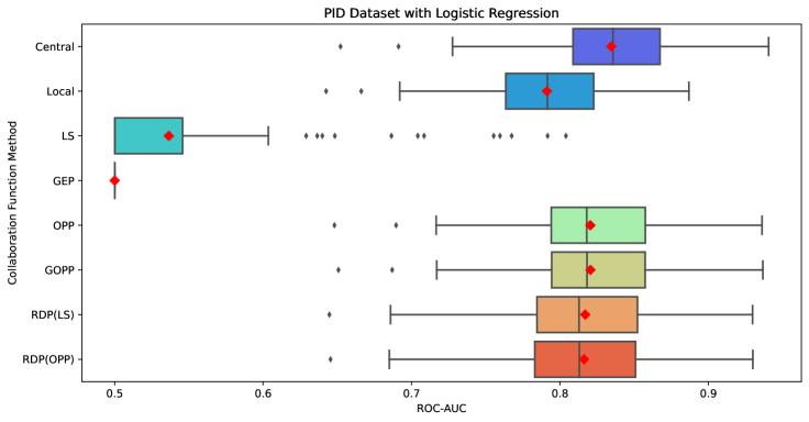
Figure 4: ROC-AUC box plot of logistic regression with PID dataset

	Central	Local	LS	GEP	OPP	GOPP	RDP(LS)	RDP(OPP)
mean	0.835	0.791	0.536	0.5	0.820	0.821	0.817	0.816
std	0.051	0.045	0.073	0.0	0.050	0.050	0.050	0.050
min	0.652	0.642	0.500	0.5	0.648	0.651	0.645	0.645
25%	0.809	0.764	0.500	0.5	0.794	0.794	0.785	0.783
50%	0.836	0.792	0.500	0.5	0.818	0.818	0.813	0.813
75%	0.867	0.823	0.546	0.5	0.857	0.857	0.852	0.851
max	0.941	0.887	0.804	0.5	0.936	0.937	0.930	0.930

Table 1: ROC-AUC statistical table of logistic regression with PID dataset

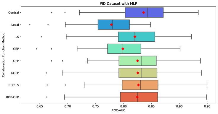
Figure 5: ROC-AUC box plot of MLP with PID dataset

	Central	Local	LS	GEP	OPP	GOPP	RDP-LS	RDP-OPP
mean	0.836	0.778	0.820	0.799	0.825	0.826	0.827	0.825
std	0.053	0.041	0.049	0.045	0.049	0.049	0.050	0.050
min	0.671	0.632	0.654	0.645	0.671	0.662	0.663	0.663
25%	0.803	0.754	0.791	0.771	0.792	0.792	0.798	0.794
50%	0.843	0.780	0.820	0.797	0.832	0.833	0.830	0.825
75%	0.871	0.811	0.856	0.831	0.859	0.860	0.862	0.861
max	0.934	0.848	0.922	0.901	0.938	0.940	0.949	0.949

Table 2: ROC-AUC statistical table of MLP with PID dataset

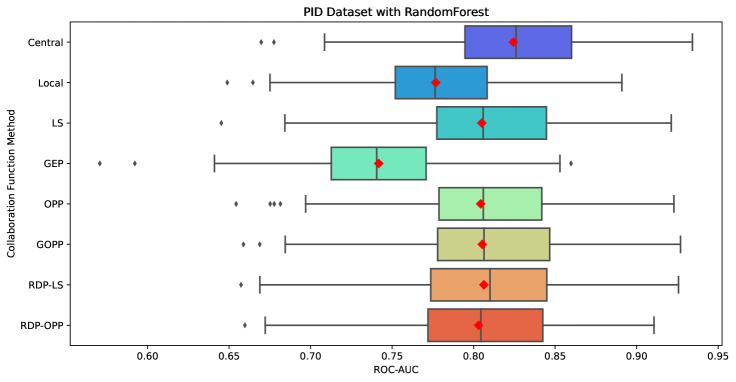
Figure 6: ROC-AUC box plot of random forest with PID dataset

	Central	Local	LS	GEP	OPP	GOPP	RDP-LS	RDP-OPP
mean	0.824	0.777	0.805	0.742	0.804	0.805	0.806	0.803
std	0.052	0.043	0.052	0.055	0.052	0.052	0.051	0.051
min	0.670	0.649	0.645	0.571	0.654	0.659	0.657	0.660
25%	0.795	0.752	0.777	0.713	0.779	0.778	0.774	0.772
50%	0.826	0.776	0.806	0.741	0.806	0.806	0.810	0.804
75%	0.860	0.808	0.845	0.771	0.842	0.847	0.845	0.842
max	0.934	0.891	0.921	0.860	0.923	0.927	0.926	0.911

Table 3: ROC-AUC statistical table of random forest with PID dataset

	LS	GEP	OPP	GOPP	RDP-LS	RDP-OPP
mean	0.033	0.007	0.025	0.038	7.886	10.356
std	0.016	0.002	0.003	0.007	1.115	3.332
min	0.023	0.006	0.022	0.030	4.931	5.870
25%	0.025	0.006	0.023	0.033	7.102	8.331
50%	0.026	0.006	0.023	0.035	7.813	9.811
75%	0.030	0.007	0.026	0.043	8.610	11.471
max	0.106	0.031	0.036	0.060	11.391	37.868

Table 4: Table of the computation time (sec) of $G_{i}$ with PID dataset

4.2.2 Heart Disease (HD) Dataset

The Heart Disease (HD) dataset [28] comprises 13 numerical features aimed at predicting the presence of heart disease. The target variable for binary classification is "TARGET," indicating the presence (1) or absence (0) of heart disease. The dataset’s features include:

1. Age : (Numerical) Patient age in years.

2. Sex: (Categorical) Gender of the patient (1 = male, 0 = female).

3. CP (Chest Pain Type): (Categorical) Type of chest pain experienced.

4. TRESTBPS: (Numerical) Resting blood pressure in mm Hg at hospital admission.

5. CHOL: (Numerical) Serum cholesterol level in mg/dl.

6. FPS (Fasting Blood Sugar): (Categorical) Indicates if fasting blood sugar is greater than 120 mg/dl (1 = true, 0 = false).

7. RESTECG: (Categorical) Results of resting electrocardiographic tests.

8. THALACH: (Numerical) Maximum heart rate achieved.

9. EXANG: (Categorical) Presence of exercise-induced angina (1 = yes, 0 = no).

10. OLDPEAK: (Numerical) ST depression induced by exercise relative to rest.

11. SLOPE: (Categorical) Slope of the peak exercise ST segment.

12. CA: (Categorical) Number of major vessels colored by fluoroscopy (0-3).

13. THAL: (Categorical) Thalassemia status (3 = normal; 6 = fixed defect; 7 = reversible defect).

14. TARGET: (Categorical) Presence (1) or absence (0) of heart disease.

For preprocessing, categorical columns in the dataset are one-hot encoded, with the first column of each category removed to avoid multicollinearity. Numerical columns are standardized for consistency. From the 1026 samples, 1000 were randomly selected, maintaining the same proportion of the target variables, to ensure a representative subset for analysis.

Box plots in Figures 7, 8, and 9 display the ROC-AUC scores for logistic regression (LR), multi-layer perceptron (MLP), and random forest (RF) models, respectively. The y-axis lists the methods used to generate collaboration functions $G_{i}$ and their associated collaborative models ($t_{i}$), alongside benchmarks of centralized (Central) and local (Local) models. The x-axis shows the ROC-AUC scores for the ML models (mean score across all workers in the local and collaborative settings). These plots highlight the effect of different collaboration function creation methods on the performance of collaborative models compared to centralized and local models in various distribution scenarios (100 random distributions for each ML model type). The red dot denotes the mean. Detailed statistical values of the ROC-AUC scores for LR, MLP, and RF are provided in Tables 5, 6, and 7, respectively. Additionally, Table 8 details the computation time (in seconds) required for each collaboration function generation method to compute all $G_{i}$ from $\tilde{X}^{\mathrm{anc}}_{i}$ across all ML model types (total of 300 iterations).

In logistic regression, Figure 7 and Table 5 show our methods outperforming local models, with LS and GEP less effective and Procrustean methods (OPP and GOPP) slightly better than RDP methods (RDP-LS and RDP-OPP). For MLP, as per Figure 8 and Table 6, LS and our approaches exceed local model performance, ranking Procrustean methods highest, followed by RDP and then LS. In the random forest analysis (Figure 9 and Table 7), only LS and Procrustean methods equaled local model performance. Computation time analysis (Table 8) revealed GEP as the most efficient, followed by OPP and LS, with RDP methods being significantly less efficient, mirroring findings from the PID dataset.

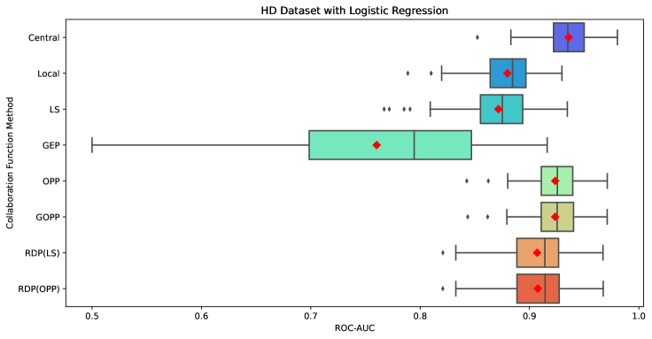
Figure 7: ROC-AUC box plot of logistic regression with HD dataset

	Central	Local	LS	GEP	OPP	GOPP	RDP(LS)	RDP(OPP)
mean	0.936	0.880	0.872	0.760	0.924	0.923	0.907	0.908
std	0.021	0.025	0.033	0.114	0.023	0.023	0.028	0.028
min	0.852	0.789	0.767	0.500	0.843	0.844	0.821	0.821
25%	0.922	0.864	0.855	0.699	0.911	0.911	0.888	0.888
50%	0.935	0.884	0.875	0.795	0.926	0.925	0.914	0.914
75%	0.950	0.897	0.894	0.847	0.940	0.940	0.927	0.927
max	0.980	0.930	0.935	0.916	0.971	0.971	0.967	0.967

Table 5: ROC-AUC statistical table of logistic regression with HD dataset

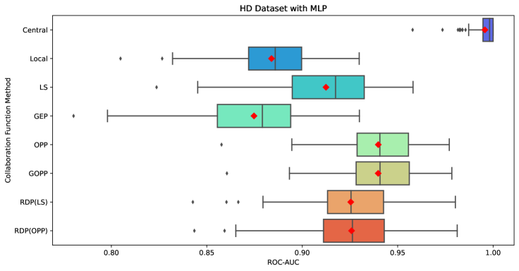
Figure 8: ROC-AUC box plot of MLP with HD dataset

	Central	Local	LS	GEP	OPP	GOPP	RDP(LS)	RDP(OPP)
mean	0.996	0.884	0.912	0.875	0.940	0.940	0.925	0.926
std	0.007	0.023	0.027	0.027	0.021	0.021	0.025	0.025
min	0.958	0.805	0.824	0.780	0.858	0.861	0.843	0.844
25%	0.995	0.872	0.895	0.856	0.929	0.928	0.913	0.911
50%	0.998	0.886	0.918	0.879	0.941	0.941	0.926	0.926
75%	1.000	0.900	0.932	0.894	0.956	0.956	0.943	0.943
max	1.000	0.930	0.958	0.930	0.977	0.978	0.980	0.981

Table 6: ROC-AUC statistical table of MLP with HD dataset

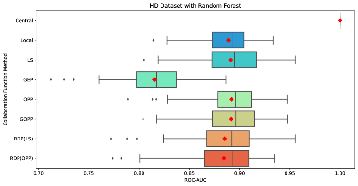
Figure 9: ROC-AUC box plot of random forest with HD dataset

	Central	Local	LS	GEP	OPP	GOPP	RDP(LS)	RDP(OPP)
mean	1.0	0.889	0.891	0.815	0.892	0.892	0.885	0.884
std	0.0	0.023	0.031	0.032	0.031	0.031	0.033	0.033
min	1.0	0.814	0.805	0.712	0.789	0.804	0.772	0.774
25%	1.0	0.873	0.872	0.798	0.878	0.873	0.867	0.865
50%	1.0	0.893	0.895	0.817	0.896	0.896	0.892	0.893
75%	1.0	0.904	0.917	0.837	0.912	0.915	0.909	0.909
max	1.0	0.934	0.955	0.886	0.948	0.948	0.955	0.935

Table 7: ROC-AUC statistical table of random forest with HD dataset

	LS	GEP	OPP	GOPP	RDP-LS	RDP-OPP
mean	0.160	0.085	0.105	0.228	66.179	72.334
std	0.084	0.023	0.012	0.031	15.941	18.276
min	0.107	0.072	0.096	0.176	0.847	51.240
25%	0.112	0.074	0.098	0.206	60.509	64.059
50%	0.115	0.076	0.099	0.221	64.613	68.302
75%	0.189	0.092	0.107	0.242	71.305	74.339
max	0.539	0.365	0.186	0.384	149.614	203.950

Table 8: Table of the computation time (sec) of $G_{i}$ with HD dataset

4.2.3 Credit-Rating Historical (CRH) Dataset

The Credit-Rating Historical (CRH) dataset is a simulated collection designed for credit rating analysis derived from MATLAB’s Statistics and Machine Learning Toolbox. The primary goal is to predict credit ratings, categorized from "AAA" to "CCC". The dataset comprises financial ratios and industry classifications:

1. WC_TA (Working Capital / Total Assets): Proportion of working capital to total assets.

2. RE_TA (Retained Earnings / Total Assets): Ratio of retained earnings to total assets.

3. EBIT_TA (Earnings Before Interests and Taxes / Total Assets): Profitability measure before interests and taxes relative to total assets.

4. MVE_BVTD (Market Value of Equity / Book Value of Total Debt): Comparison of equity market value to total debt book value.

5. S_TA (Sales / Total Assets): Ratio of total sales to total assets.

6. Industry: Numerical labels (1-12) for industry sectors.

7. Rating: Credit ratings: "AAA", "AA", "A", "BBB", "BB", "B", "CCC".

Preprocessing includes one-hot encoding of the "Industry" column, removing the first category to prevent multicollinearity. Numerical columns are standardized. The target variable, "Rating," is binarized: ratings "BBB" and above are labeled 1, and lower ratings are labeled 0. From the total 3932 samples, 1000 were randomly selected, ensuring representation across target variables for analysis.

Box plots in Figures 10, 11, and 12 display the ROC-AUC scores for logistic regression (LR), multi-layer perceptron (MLP), and random forest (RF) models, respectively. The y-axis lists the methods used to generate collaboration functions $G_{i}$ and their associated collaborative models ($t_{i}$), alongside benchmarks of centralized (Central) and local (Local) models. The x-axis shows the ROC-AUC scores for the ML models (mean score across all workers in the local and collaborative settings). These plots highlight the effect of different collaboration function creation methods on the performance of collaborative models compared to centralized and local models in various distribution scenarios (100 random distributions for each ML model type). The red dot denotes the mean. Detailed statistical values of the ROC-AUC scores for LR, MLP, and RF are provided in Tables 9, 10, and 11, respectively. Additionally, Table 12 details the computation time (in seconds) required for each collaboration function generation method to compute all $G_{i}$ from $\tilde{X}^{\mathrm{anc}}_{i}$ across all ML model types (total of 300 iterations).

In logistic regression, Figure 7 and Table 5 show that only Procrustean methods (OPP and GOPP) surpassed local model performance. For MLP, as demonstrated in Figure 8 and Table 6, all collaborative methods outdid the local models, with RDP methods leading, followed closely by Procrustean methods, then LS, and finally GEP. Figure 9 and Table 7 indicate that collaborative methods did not exceed local model performance in the random forest analysis. Computation time analysis (Table 12) mirrors findings from the PID and HD datasets, with GEP being the most time-efficient, followed by OPP and LS, while RDP methods are significantly less efficient.

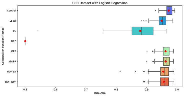
Figure 10: ROC-AUC box plot of logistic regression with CRH dataset

	Central	Local	LS	GEP	OPP	GOPP	RDP-LS	RDP-OPP
mean	0.973	0.950	0.879	0.5	0.963	0.963	0.955	0.957
std	0.014	0.021	0.058	0.0	0.017	0.017	0.027	0.021
min	0.930	0.885	0.542	0.5	0.902	0.901	0.813	0.890
25%	0.966	0.941	0.852	0.5	0.955	0.956	0.946	0.946
50%	0.974	0.953	0.883	0.5	0.964	0.965	0.960	0.960
75%	0.984	0.964	0.922	0.5	0.975	0.976	0.973	0.973
max	0.993	0.986	0.965	0.5	0.989	0.989	0.990	0.990

Table 9: ROC-AUC statistical table of logistic regression with CRH dataset

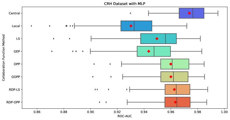
Figure 11: ROC-AUC box plot of MLP with CRH dataset

	Central	Local	LS	GEP	OPP	GOPP	RDP-LS	RDP-OPP
mean	0.974	0.930	0.950	0.943	0.960	0.960	0.963	0.963
std	0.014	0.022	0.022	0.023	0.017	0.017	0.017	0.016
min	0.930	0.856	0.872	0.871	0.903	0.902	0.903	0.907
25%	0.966	0.923	0.937	0.935	0.952	0.952	0.956	0.956
50%	0.976	0.933	0.956	0.947	0.961	0.962	0.964	0.964
75%	0.985	0.946	0.964	0.960	0.974	0.973	0.974	0.974
max	0.995	0.972	0.982	0.983	0.985	0.985	0.988	0.987

Table 10: ROC-AUC statistical table of MLP with CRH dataset

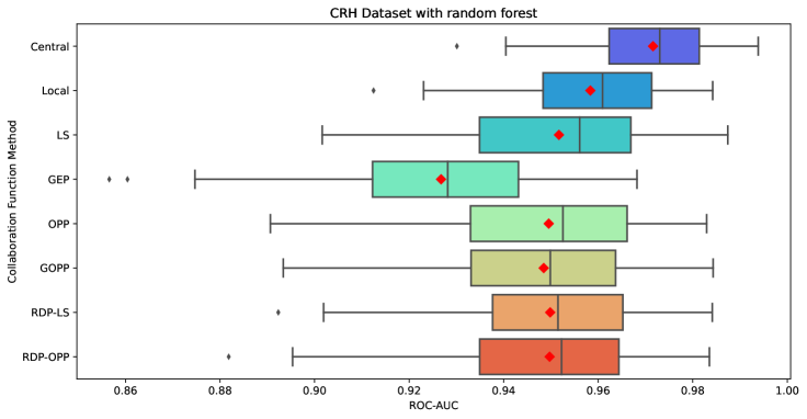
Figure 12: ROC-AUC box plot of random forest with CRH dataset

	Central	Local	LS	GEP	OPP	GOPP	RDP-LS	RDP-OPP
mean	0.972	0.958	0.952	0.927	0.950	0.948	0.950	0.950
std	0.013	0.016	0.020	0.024	0.021	0.022	0.020	0.020
min	0.930	0.912	0.902	0.857	0.891	0.893	0.892	0.882
25%	0.962	0.948	0.935	0.912	0.933	0.933	0.938	0.935
50%	0.973	0.961	0.956	0.928	0.953	0.950	0.952	0.952
75%	0.981	0.971	0.967	0.943	0.966	0.964	0.965	0.964
max	0.994	0.984	0.987	0.968	0.983	0.984	0.984	0.984

Table 11: ROC-AUC statistical table of random forest with CRH dataset

	LS	GEP	OPP	GOPP	RDP-LS	RDP-OPP
mean	0.090	0.057	0.075	0.222	23.157	23.759
std	0.023	0.034	0.007	0.064	8.031	8.503
min	0.074	0.035	0.069	0.144	0.736	2.046
25%	0.076	0.036	0.071	0.184	20.274	19.143
50%	0.079	0.037	0.072	0.206	22.484	21.970
75%	0.094	0.076	0.078	0.234	24.830	25.432
max	0.254	0.170	0.162	0.636	80.653	87.054

Table 12: Table of the computation time (sec) of $G_{i}$ with CRH dataset

4.3 Discussions

From the overall numerical experiment results, we observed that Procrustean-based methods generally excelled in recognition performance across various datasets and ML models, affirming our hypothesis that preserving the structure of intermediate representations for model performance is critical. The constraint of $G_{i}$ to the orthogonal matrix manifold significantly contributed to this effectiveness. However, RDP methods outperformed in some instances (11, 10), suggesting that minimizing alignment error can be more crucial in some scenarios despite potential structure distortion. Notably, the choice of initial points in the RDP method did not lead to significant performance variations. Likewise, no substantial differences were observed between OPP and GOPP despite their differences in incorporating the target matrix $Z$ in optimization. This finding prompts further investigation into GOPP’s optimization landscape and the practicality of using dominant singular vectors as the target matrix, thus providing a vital avenue for future theoretical research.

Regarding computation time, GEP consistently emerged as the most efficient collaboration method, followed by OPP, LS, GOPP, and RDP methods, which were significantly less efficient. Using the Big-$O$ notation, GEP’s computational time complexity is $O(r(\tilde{m}N)^{2}+(\tilde{m}N)^{3})$, with the first term representing the time complexity up to formulating the generalized eigenvalue problem, and the second term for solving it [64]. For OPP and LS, the complexities are $O(r\tilde{m}N\min(r,\tilde{m}N)+N(r\tilde{m}\min(r,\tilde{m})+r\tilde{m}^{2})$ and $O(r\tilde{m}N\min(r,\tilde{m}N)+N(r\tilde{m}^{2}+2\tilde{m}^{3})$, respectively [37]. Both methods involve computing the target matrix $Z$ via SVD, represented by the first term. The difference arises in the second term: OPP computes the SVD of $Z^{\top}\tilde{X}^{\mathrm{anc}}_{i}\in\mathbb{R}^{\tilde{m}\times\tilde{m}}$, while LS calculates the Moore-Penrose inverse of $\tilde{X}^{\mathrm{anc}}_{i}\in\mathbb{R}^{r\times\tilde{m}}$. Given that the dominant complexity in Moore-Penrose inversion is SVD, and considering $\tilde{m}<<r$ in our experiment settings, this accounts for the faster performance of OPP compared to LS. GEP’s efficiency advantage is due to the second term being $r$-independent.

Our experimental results conclude that the OPP method is the most practical collaboration function creation method in addressing our research question. It has proved to enhance the performance and stability of collaborative models, maintaining computational efficiency and aligning with the non-iterative communication and privacy tenets of the DC framework.

5 Conclusion

We introduced innovative methods for creating collaboration functions within the NRI-DC framework, focusing on preserving the structure of intermediate representations. We established the necessary conditions for practical collaboration functions and built our proposed methods on these conditions, ensuring a solid theoretical foundation. Our methods can be divided into two categories: those formulated over the orthogonal matrix manifold and those formulated over the full-rank manifold. The orthogonal matrix manifold formulation benefits from established Procrustean analysis methods, while the full-rank manifold formulation is amenable to Riemannian optimization algorithms, proving efficient approaches for these formulations. Through empirical analysis of three public datasets using diverse machine learning models, we found that the orthogonal matrix manifold formulation, particularly with the orthogonal Procrustes solution, excels in practical application, consistently enhancing model performance with efficiency.

Future research directions include strengthening the theoretical foundation of this study. A fundamental assumption is the exclusive use of linear dimensionality reduction functions like PCA. However, to more effectively capture the structure of original data matrices, exploring alternatives like LPP [17] or tSNE [18] is necessary, potentially requiring reevaluation of the origin shifts and the current target matrix $Z$ setting. Another crucial area for exploration is the privacy-preserving aspect of the NRI-DC framework. Further assessing its vulnerabilities and ensuring strict compliance with global privacy regulations are vital for its broader societal application. Alternatively, clarifying the framework’s privacy limits may lead to optimizing the framework for enhanced simplicity and efficiency without undermining privacy protections, which is a significant area of future research.

References

- [1] Abbas Acar, Hidayet Aksu, A Selcuk Uluagac, and Mauro Conti. A survey on homomorphic encryption schemes: Theory and implementation. ACM Computing Surveys (Csur), 51(4):1–35, 2018.
- [2] Eugene Bagdasaryan, Andreas Veit, Yiqing Hua, Deborah Estrin, and Vitaly Shmatikov. How to backdoor federated learning. In International conference on artificial intelligence and statistics, pages 2938–2948. PMLR, 2020.
- [3] Aner Ben-Efraim, Yehuda Lindell, and Eran Omri. Optimizing semi-honest secure multiparty computation for the internet. In Proceedings of the 2016 ACM SIGSAC Conference on Computer and Communications Security, pages 578–590, 2016.
- [4] Keith Bonawitz, Vladimir Ivanov, Ben Kreuter, Antonio Marcedone, H Brendan McMahan, Sarvar Patel, Daniel Ramage, Aaron Segal, and Karn Seth. Practical secure aggregation for privacy-preserving machine learning. In proceedings of the 2017 ACM SIGSAC Conference on Computer and Communications Security, pages 1175–1191, 2017.
- [5] Nicolas Boumal. An introduction to optimization on smooth manifolds. Cambridge University Press, 2023.
- [6] Nicolas Boumal, Bamdev Mishra, P-A Absil, and Rodolphe Sepulchre. Manopt, a matlab toolbox for optimization on manifolds. The Journal of Machine Learning Research, 15(1):1455–1459, 2014.
- [7] David Chaum. The dining cryptographers problem: Unconditional sender and recipient untraceability. Journal of cryptology, 1:65–75, 1988.
- [8] David L Chaum. Untraceable electronic mail, return addresses, and digital pseudonyms. Communications of the ACM, 24(2):84–90, 1981.
- [9] Cynthia Dwork. Differential privacy: A survey of results. In International conference on theory and applications of models of computation, pages 1–19. Springer, 2008.
- [10] Tom Fawcett. An introduction to roc analysis. Pattern recognition letters, 27(8):861–874, 2006.
- [11] Matt Fredrikson, Somesh Jha, and Thomas Ristenpart. Model inversion attacks that exploit confidence information and basic countermeasures. In Proceedings of the 22nd ACM SIGSAC conference on computer and communications security, pages 1322–1333, 2015.
- [12] Karl Pearson F.R.S. Liii. on lines and planes of closest fit to systems of points in space. The London, Edinburgh, and Dublin Philosophical Magazine and Journal of Science, 2(11):559–572, 1901.
- [13] Karan Ganju, Qi Wang, Wei Yang, Carl A Gunter, and Nikita Borisov. Property inference attacks on fully connected neural networks using permutation invariant representations. In Proceedings of the 2018 ACM SIGSAC conference on computer and communications security, pages 619–633, 2018.
- [14] Adrià Gascón, Phillipp Schoppmann, Borja Balle, Mariana Raykova, Jack Doerner, Samee Zahur, and David Evans. Privacy-preserving distributed linear regression on high-dimensional data. Cryptology ePrint Archive, Paper 2016/892, 2016. https://eprint.iacr.org/2016/892.
- [15] John C Gower and Garmt B Dijksterhuis. Procrustes problems, volume 30. OUP Oxford, 2004.
- [16] Simon Haykin. Neural networks: a comprehensive foundation. Prentice Hall PTR, 1994.
- [17] Xiaofei He and Partha Niyogi. Locality preserving projections. Advances in neural information processing systems, 16, 2003.
- [18] Geoffrey E Hinton and Sam Roweis. Stochastic neighbor embedding. Advances in neural information processing systems, 15, 2002.
- [19] Tin Kam Ho. Random decision forests. In Proceedings of 3rd international conference on document analysis and recognition, volume 1, pages 278–282. IEEE, 1995.
- [20] Hongsheng Hu, Zoran Salcic, Lichao Sun, Gillian Dobbie, Philip S Yu, and Xuyun Zhang. Membership inference attacks on machine learning: A survey. ACM Computing Surveys (CSUR), 54(11s):1–37, 2022.
- [21] Wen Huang, P-A Absil, and Kyle A Gallivan. A riemannian bfgs method without differentiated retraction for nonconvex optimization problems. SIAM Journal on Optimization, 28(1):470–495, 2018.
- [22] Akira Imakura, Anna Bogdanova, Takaya Yamazoe, Kazumasa Omote, and Tetsuya Sakurai. Accuracy and privacy evaluations of collaborative data analysis. arXiv preprint arXiv:2101.11144, 2021.
- [23] Akira Imakura, Hiroaki Inaba, Yukihiko Okada, and Tetsuya Sakurai. Interpretable collaborative data analysis on distributed data. Expert Systems with Applications, 177:114891, 2021.
- [24] Akira Imakura and Tetsuya Sakurai. Data collaboration analysis framework using centralization of individual intermediate representations for distributed data sets. ASCE-ASME Journal of Risk and Uncertainty in Engineering Systems, Part A: Civil Engineering, 6(2):04020018, 2020.
- [25] Akira Imakura, Tetsuya Sakurai, Yukihiko Okada, Tomoya Fujii, Teppei Sakamoto, and Hiroyuki Abe. Non-readily identifiable data collaboration analysis for multiple datasets including personal information. Information Fusion, 98:101826, 2023.
- [26] Akira Imakura, Xiucai Ye, and Tetsuya Sakurai. Collaborative data analysis: Non-model sharing-type machine learning for distributed data. In Knowledge Management and Acquisition for Intelligent Systems: 17th Pacific Rim Knowledge Acquisition Workshop, PKAW 2020, Yokohama, Japan, January 7–8, 2021, Proceedings 17, pages 14–29. Springer, 2021.
- [27] Akira Imakura, Xiucai Ye, and Tetsuya Sakurai. Collaborative novelty detection for distributed data by a probabilistic method. In Vineeth N. Balasubramanian and Ivor Tsang, editors, Proceedings of The 13th Asian Conference on Machine Learning, volume 157 of Proceedings of Machine Learning Research, pages 932–947. PMLR, 17–19 Nov 2021.
- [28] Steinbrunn William Pfisterer Matthias Janosi, Andras and Robert Detrano. Heart Disease. UCI Machine Learning Repository, 1988. DOI: https://doi.org/10.24432/C52P4X.
- [29] Peter Kairouz, H Brendan McMahan, Brendan Avent, Aurélien Bellet, Mehdi Bennis, Arjun Nitin Bhagoji, Kallista Bonawitz, Zachary Charles, Graham Cormode, Rachel Cummings, et al. Advances and open problems in federated learning. Foundations and Trends® in Machine Learning, 14(1–2):1–210, 2021.
- [30] Sai Praneeth Karimireddy, Satyen Kale, Mehryar Mohri, Sashank Reddi, Sebastian Stich, and Ananda Theertha Suresh. SCAFFOLD: Stochastic controlled averaging for federated learning. In Hal Daumé III and Aarti Singh, editors, Proceedings of the 37th International Conference on Machine Learning, volume 119 of Proceedings of Machine Learning Research, pages 5132–5143. PMLR, 13–18 Jul 2020.
- [31] Jakub Konečnỳ, H Brendan McMahan, Felix X Yu, Peter Richtárik, Ananda Theertha Suresh, and Dave Bacon. Federated learning: Strategies for improving communication efficiency. arXiv preprint arXiv:1610.05492, 2016.
- [32] Qinbin Li, Yiqun Diao, Quan Chen, and Bingsheng He. Federated learning on non-iid data silos: An experimental study. In 2022 IEEE 38th International Conference on Data Engineering (ICDE), pages 965–978. IEEE, 2022.
- [33] Qinbin Li, Zeyi Wen, Zhaomin Wu, Sixu Hu, Naibo Wang, Yuan Li, Xu Liu, and Bingsheng He. A survey on federated learning systems: Vision, hype and reality for data privacy and protection. IEEE Transactions on Knowledge and Data Engineering, 2021.
- [34] Tian Li, Anit Kumar Sahu, Ameet Talwalkar, and Virginia Smith. Federated learning: Challenges, methods, and future directions. IEEE signal processing magazine, 37(3):50–60, 2020.
- [35] Tian Li, Anit Kumar Sahu, Manzil Zaheer, Maziar Sanjabi, Ameet Talwalkar, and Virginia Smith. Federated optimization in heterogeneous networks, 2020.
- [36] Xiang Li, Kaixuan Huang, Wenhao Yang, Shusen Wang, and Zhihua Zhang. On the convergence of fedavg on non-iid data. arXiv preprint arXiv:1907.02189, 2019.
- [37] Xiaocan Li, Shuo Wang, and Yinghao Cai. Tutorial: Complexity analysis of singular value decomposition and its variants, 2019.
- [38] Tao Lin, Lingjing Kong, Sebastian U Stich, and Martin Jaggi. Ensemble distillation for robust model fusion in federated learning. Advances in Neural Information Processing Systems, 33:2351–2363, 2020.
- [39] Shuyang Ling. Generalized power method for generalized orthogonal procrustes problem: global convergence and optimization landscape analysis. arXiv preprint arXiv:2106.15493, 2021.
- [40] Shuyang Ling. Near-optimal bounds for generalized orthogonal procrustes problem via generalized power method. arXiv preprint arXiv:2112.13725, 2021.
- [41] Lingjuan Lyu, Han Yu, and Qiang Yang. Threats to federated learning: A survey. arXiv preprint arXiv:2003.02133, 2020.
- [42] Paulo Martins, Leonel Sousa, and Artur Mariano. A survey on fully homomorphic encryption: An engineering perspective. ACM Computing Surveys (CSUR), 50(6):1–33, 2017.
- [43] Brendan McMahan, Eider Moore, Daniel Ramage, Seth Hampson, and Blaise Aguera y Arcas. Communication-efficient learning of deep networks from decentralized data. In Artificial intelligence and statistics, pages 1273–1282. PMLR, 2017.
- [44] Akihiro Mizoguchi, Anna Bogdanova, Akira Imakura, and Tetsuya Sakurai. Data collaboration analysis applied to compound datasets and the introduction of projection data to non-iid settings, 2023.
- [45] Akihiro Mizoguchi, Akira Imakura, and Tetsuya Sakurai. Application of data collaboration analysis to distributed data with misaligned features. Informatics in Medicine Unlocked, 32:101013, 2022.
- [46] Hung Nguyen, Di Zhuang, Pei-Yuan Wu, and Morris Chang. Autogan-based dimension reduction for privacy preservation. Neurocomputing, 384:94–103, 2020.
- [47] Keiyu Nosaka and Akiko Yoshise. Creating collaborative data representations using matrix manifold optimal computation and automated hyperparameter tuning. In 2023 IEEE 3rd International Conference on Electronic Communications, Internet of Things and Big Data (ICEIB), pages 180–185. IEEE, 2023.
- [48] Fabian Pedregosa, Gaël Varoquaux, Alexandre Gramfort, Vincent Michel, Bertrand Thirion, Olivier Grisel, Mathieu Blondel, Peter Prettenhofer, Ron Weiss, Vincent Dubourg, et al. Scikit-learn: Machine learning in python. Journal of machine learning research, 12(Oct):2825–2830, 2011.
- [49] Amirhossein Reisizadeh, Farzan Farnia, Ramtin Pedarsani, and Ali Jadbabaie. Robust federated learning: The case of affine distribution shifts. Advances in Neural Information Processing Systems, 33:21554–21565, 2020.
- [50] Pierangelo Rosati, Peter Deeney, Mark Cummins, Lisa van der Werff, and Theo Lynn. Social media and stock price reaction to data breach announcements: Evidence from us listed companies. Research in International Business and Finance, 47:458–469, 2019.
- [51] Bita Darvish Rouhani, M. Sadegh Riazi, and Farinaz Koushanfar. Deepsecure: Scalable provably-secure deep learning. Cryptology ePrint Archive, Paper 2017/502, 2017. https://eprint.iacr.org/2017/502.
- [52] Ashish P Sanil, Alan F Karr, Xiaodong Lin, and Jerome P Reiter. Privacy preserving regression modelling via distributed computation. In Proceedings of the tenth ACM SIGKDD international conference on Knowledge discovery and data mining, pages 677–682, 2004.
- [53] Peter H Schönemann. A generalized solution of the orthogonal procrustes problem. Psychometrika, 31(1):1–10, 1966.
- [54] Latanya Sweeney. k-anonymity: A model for protecting privacy. International journal of uncertainty, fuzziness and knowledge-based systems, 10(05):557–570, 2002.
- [55] Stacey Truex, Nathalie Baracaldo, Ali Anwar, Thomas Steinke, Heiko Ludwig, Rui Zhang, and Yi Zhou. A hybrid approach to privacy-preserving federated learning. In Proceedings of the 12th ACM workshop on artificial intelligence and security, pages 1–11, 2019.
- [56] Bart Vandereycken. Low-rank matrix completion by riemannian optimization. SIAM Journal on Optimization, 23(2):1214–1236, 2013.
- [57] Thomas Viklands. Algorithms for the weighted orthogonal procrustes problem and other least squares problems. PhD thesis, Datavetenskap, 2006.
- [58] Xiao Wang, Samuel Ranellucci, and Jonathan Katz. Global-scale secure multiparty computation. In Proceedings of the 2017 ACM SIGSAC Conference on Computer and Communications Security, pages 39–56, 2017.
- [59] Runhua Xu, Nathalie Baracaldo, and James Joshi. Privacy-preserving machine learning: Methods, challenges and directions. arXiv preprint arXiv:2108.04417, 2021.
- [60] Timothy Yang, Galen Andrew, Hubert Eichner, Haicheng Sun, Wei Li, Nicholas Kong, Daniel Ramage, and Françoise Beaufays. Applied federated learning: Improving google keyboard query suggestions. arXiv preprint arXiv:1812.02903, 2018.
- [61] Andrew C Yao. Protocols for secure computations. In 23rd annual symposium on foundations of computer science (sfcs 1982), pages 160–164. IEEE, 1982.
- [62] Jasmin Zalonis, Frederik Armknecht, Björn Grohmann, and Manuel Koch. Report: State of the art solutions for privacy preserving machine learning in the medical context, 2022.
- [63] Ligeng Zhu, Zhijian Liu, and Song Han. Deep leakage from gradients. Advances in neural information processing systems, 32, 2019.
- [64] 川上雄大. データコラボレーション解析における統合関数最適化問題の定式化と効率的解法, 2022年度 筑波大学大学院 博士前期課程 理工情報生命学術院 システム情報工学研究群 社会工学学位プログラム 修士論文.