Fast, Scale-Adaptive, and Uncertainty-Aware Downscaling of Earth System Model Fields with Generative Foundation Models

Abstract

Accurate and high-resolution Earth system model (ESM) simulations are essential to assess the ecological and socio-economic impacts of anthropogenic climate change, but are computationally too expensive. Recent machine learning approaches have shown promising results in downscaling ESM simulations, outperforming state-of-the-art statistical approaches.
However, existing methods require computationally costly retraining for each ESM and extrapolate poorly to climates unseen during training. We address these shortcomings by learning a consistency model (CM) that efficiently and accurately downscales arbitrary ESM simulations without retraining in a zero-shot manner.
Our foundation model approach yields probabilistic downscaled fields at resolution only limited by the observational reference data. We show that the CM outperforms state-of-the-art diffusion models at a fraction of computational cost while maintaining high controllability on the downscaling task. Further, our method generalizes to climate states unseen during training without explicitly formulated physical constraints.

1 Introduction

Accurate and high-resolution climate simulations are of crucial importance to project the climatic, hydrological, ecological, and socioeconomic impacts of anthropogenic climate change. Precipitation, in particular, is one of the most important climate variables, with huge impacts, e.g., on vegetation and crop yields, infrastructure, or the economy [Kotz et al., 2022]. However, it is also the variable that is arguably most difficult to model and predict, especially extreme precipitation events. Numerical Earth system models (ESMs) are our main tool to project the future evolution of precipitation and its extremes. However, they exhibit biases and have much coarser spatial resolution, on the order of 10-100km, than needed for reliable assessments of the impacts of climate change [Schneider et al., 2017].

Due to the chaotic nature of geophysical fluid dynamics, the trajectory of climate simulations will not match historical observations, requiring approaches suitable for unpaired samples to learn such tasks. Recently, methods from generative deep learning have shown promising results in downscaling or correcting spatial patterns in ESM simulations. Normalizing flows (NFs) [Dinh et al., 2015] and generative adversarial networks (GANs) [Goodfellow et al., 2014] can perform these tasks efficiently in a single step [Groenke et al., 2020, Pan et al., 2021, François et al., 2021, Harris et al., 2022, Hess et al., 2022, Hess et al., 2023]. However, NFs often exhibit lower quality in the generated images, while GANs can suffer from training instabilities and problems such as mode collapse [Arjovsky and Bottou, 2017]. Moreover, these approaches require computationally expensive retraining of the neural networks for each ESM to be processed. This makes downscaling large ESM ensembles, as needed in impact assessments, prohibitively costly and time-consuming.

Diffusion-based generative models have demonstrated superior performance over NFs and GANs on classical image generation tasks [Dhariwal and Nichol, 2021, Song et al., 2021]. Crucially, iteratively solving the reversed diffusion equation allows for strong control over the image sampling process. This enables so-called foundation models that are only trained on a given target dataset and which can later be repurposed, e.g., to generate realistic images based on a given “stroke sketch” guide as in SDEdit [Meng et al., 2022].

So far, such foundation model-based approaches have only been applied to downscale idealized fluid dynamics [Bischoff and Deck, 2023, Wan et al., 2023] in Earth system science-related tasks. Both studies use stochastic differential equation (SDE) based diffusion models and achieve remarkable performance. The iterative integration of the SDE, however, implies that the generative network needs to be evaluated up to 1000 times in order to downscale a single simulated field. This makes such methods unsuitable for processing large simulation datasets, e.g., at high temporal resolution or over long periods, as would be needed in the context of climate change projections and impact assessments.

In this work, we tackle these shortcomings using a novel type of generative approach based on consistency models (CM) [Song et al., 2023] to downscale global precipitation simulations from a fully-coupled ESM in a single step, without sacrifices in performance or the controllability of the sampling. We train the CM network from scratch (“in isolation”) on ERA5 reanalysis data only, making the training independent of any ESM. In summary, our study makes the following contributions:

• Our foundation model is trained on the target dataset only, without conditioning on the ESM. This makes our method applicable to any ESM without requiring computationally expensive retraining.

• The training is much more stable than in previous methods based on CycleGAN [Zhu et al., 2017, Pan et al., 2021, François et al., 2021, Hess et al., 2022, Hess et al., 2023]).

• The generative downscaling is controllable at the inference stage after training, so that the downscaled fields preserve spatial patterns of the ESM up to a chosen characteristic spatial scale.

• The consistency model employed here is up to three orders of magnitude faster than current state-of-the-art diffusion model-based approaches [Bischoff and Deck, 2023], yet shows superior performance.

• The highly efficient CM allows the generation of a large number of downscaled realizations for a single ESM field (i.e., a one-to-many mapping), enabling a robust quantification of the sampling spread.

• Our method is robust to out-of-sample predictions, showing strong preservation of the non-stationary dynamics in future transient climates (e.g., in an extreme SSP5-8.5 scenario). This is a big advantage over previous deep learning-based methods that require specifically formulated physical constraints in order to generalize [Beucler et al., 2021, Harder et al., 2022, Hess et al., 2022].

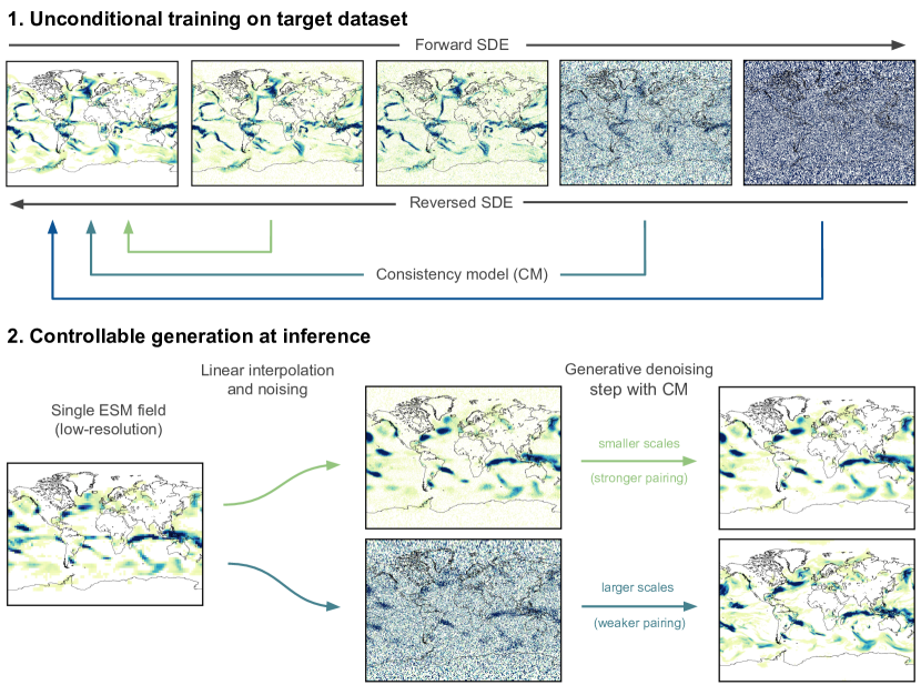
Figure 1: Sketch of the foundation model for downscaling of Earth system model fields. (Upper panel) Unconditional training of the score-based diffusion and consistency models (CM) that learn to reverse a forward diffusion process. While the stochastic differential equation of the diffusion model requires an iterative integration over many steps, the CM only takes a single step to generate a global precipitation field from noise. (Lower panel) The unconditionally trained foundation model is used to downscale (upsample) a low-resolution ESM precipitation field to a four times higher resolution. By adding noise of a chosen variance to the ESM field, the spatial scale to be preserved in the ESM can be controlled: small noise variance implies a close pairing to the original ESM field with only small changes; a larger variance will result in changes of larger spatial scales and in weaker pairing to the ESM field.

2 Results

We evaluate the efficient consistency model-based downscaling method against the SDE bridge from [Bischoff and Deck, 2023] over the test set data. We investigate the performance of the downscaling, the ability to correct distributional biases in the ESM, the sample spread given a chosen spatial scale, and the preservation of trends in future climate scenarios.

2.1 Downscaling Spatial Fields

For a qualitative comparison, we show single precipitation fields in Fig. 2. Both generative downscaling methods based on the SDE bridge (Fig. 2E) or CM (Fig. 2G) are able to produce high-resolution precipitation fields that are visually indistinguishable from the unpaired ERA5 field (Fig. 2A).

When upscaled back to the native POEM resolution using a $4\times 4$-kernel average pooling, an accurate representation of the low-resolution POEM simulation field is apparent. As indicated in Fig. 2F and Fig. 2H, a high Pearson correlation of $0.89$ and $0.95$ for the SDE and CM methods, respectively, is maintained between upscaled corrected and native fields.

We provide correlation statistics for the entire test set in Table LABEL:tab:correlation. Besides the average pooled fields, we also compare the downscaled and linearly interpolated POEM simulation on the high-resolution grid by applying a low-pass filter with a cut-off frequency set to $k^{*}=0.0667$ on the downscaled fields before computing the correlation. In this way we compare the preservation of the large-scale patterns in the ESM. The SDE bridge achieves a mean correlation of $0.918$ and $0.916$ for the average pooled and low-pass filtered fields, respectively. Our CM-based method achieves even higher correlation values of $0.954$ and $0.941$ for both measures.

We estimate the average time it takes to produce a single sample with the SDE and CM methods on a NVIDIA V100 32GB GPU. The average is taken over $100$ samples and we set the number of SDE integration steps to $500$ as in [Bischoff and Deck, 2023], which is lower then the typical $1000-2000$ steps. The SDE takes on average $39.355$ seconds, while the CM samples much more efficiently taking only $0.116$ seconds.

We analyze the downscaling performance of the CM and SDE bridge approaches quantitatively using power spectral densities (PSDs) as in [Ravuri et al., 2021, Hess et al., 2023]. The ESM fields under-represent variability at small spatial scales. This implies an underestimation of spatial intermittency, i.e., overly smooth precipitation patterns. This issue is well known and presents a key problem for the assessment of the impacts of extreme precipitation in a changing climate. The generative downscaling methods based on SDEs and CM perform very well in increasing spatial resolution and greatly improve the spatial intermittency at the smaller spatial scales (Fig. 3A).

We also investigate the change in PSDs as a function of the noise variance schedule time $t$ in Fig. 3B, which is associated with the spatial scale up to which patterns are corrected, as explained in the Methods section. For minimal noise, i.e., $t^{*}=t_{\mathrm{min}}$, the CM model reproduces the PSD of the ESM as one would expect, as there are no changes made to the ESM field. For maximal variance with $t^{*}=t_{\mathrm{max}}$, the PSD closely matches the ERA5 reanalysis ground truth. For any $t_{\mathrm{min}}<t^{*}<t_{\mathrm{max}}$, we find a trade-off between the two extreme cases that match the PSD above and below the intersection (dotted grey line) to a certain degree, depending on the spatial scale preserved in the ESM.

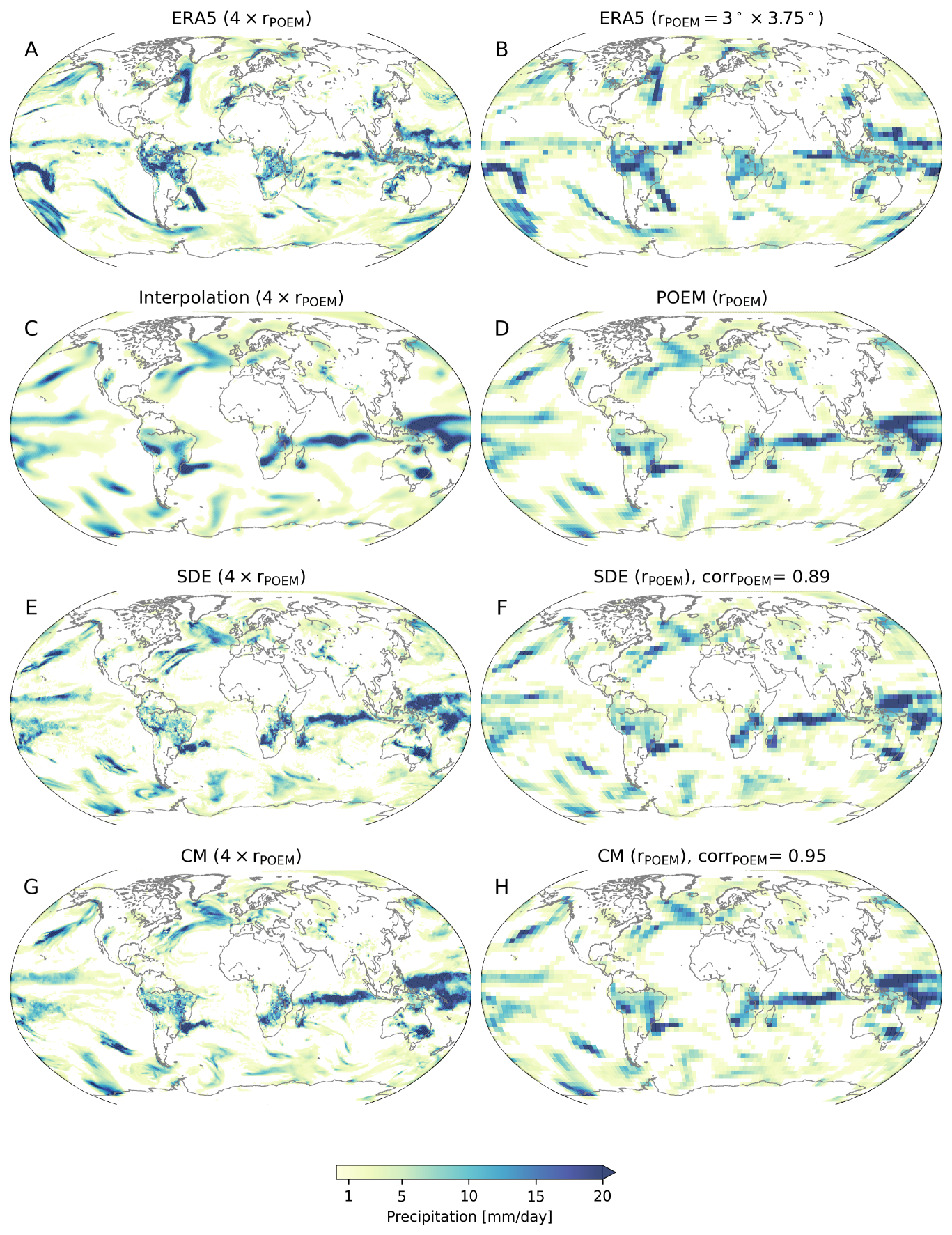
Figure 2: Qualitative comparison of single-day precipitation fields. (A) Daily precipitation from the ERA5 target datasets was used for training the generative foundation models, and (B) at four times lower resolution for comparisons. (C) A precipitation field from a historical run of the POEM ESM interpolated to the target resolution and (D) on its native resolution of $3^{\circ}\times 3.75^{\circ}$. The POEM fields is unpaired with the ERA5 field from the same date or any other ERA5 field. (E) Downscaled field from POEM (D) with the SDE bridge method. (F) An upscaled (average pooled) representation of (E) for comparison with the original POEM field shown in D and the Pearson correlation between the two. In (G) and (H), the respective fields for the CM method are shown. Note that the CM downscaling yields a higher correlation, and hence better consistency of the large-scale features, than the SDE method.

Table 1: Summary statistics comparing our CM approach and the SDE bridge as benchmark. Correlations are computed (2nd column) on the native POEM grid ($r=3^{\circ}\times 3.75^{\circ})$ by applying a $4\times 4$ average pooling to the downscaled fields and (3rd column) on the downscaled grid by applying a low-pass filter to the high-resolution downscaled fields with a cut-off frequency that is consistent with the chosen spatial scale in POEM to be preserved. (4th column) The global long-term mean absolute error with respect to ERA5 and (5th column) the respective error reduction compared to the POEM ESM bias. (6th column) The global absolute error in the 95^th precipitation percentile and (7th column) the error reduction with respect to the POEM ESM bias. An estimation of the mean sampling time is also reported (8th column). CM shows a comparable or better performance than the SDE bridge despite being much more efficient computationally.

Model	Correlation (pooled)	Correlation (low-pass)	Mean error	%	95th precentile error	%	Sample time [s]
SDE	0.918	0.916	0.214	72.51	1.106	68.15	39.355
CM	0.954	0.941	0.217	72.08	1.080	68.92	0.116

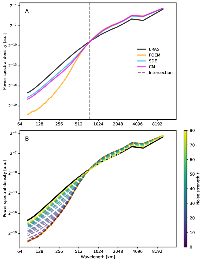
Figure 3: Mean spatial power spectral densities (PSDs) of global precipitation fields. (A) Comparison of the PSDs for the target ERA5 reanalysis data (black), the POEM simulations interpolated to the same high-resolution grid (orange), the SDE bridge (cyan), and the CM downscaling (magenta). The vertical dashed lines marks the spatial scale at which the PSDs of POEM and ERA5 intersect and is thus a natural choice for for the wavenumber $k^{\ast}$ up to which to correct, which in turn determines $t^{\ast}$, i.e. the noising strength in the diffusion models (see Eq. 8 in the Methods). (B) CM downscaling (dashed lines) applied to be consistent with different spatial scales as a function of the noising strength $t$ over the entire range $[t_{\mathrm{min}},t_{\mathrm{max}}]$. Noising small scales implies nearly reproducing the POEM simulations while noising larger scales corresponds to a weaker pairing to the ESM (see Fig. 1).

2.2 Bias Correction

We compare the ability to correct biases in the ESM with histograms of relative frequency and latitude-profiles of mean precipitation to investigate the reduction of known biases such as a double-ITCZ [Tian and Dong, 2020], following the evaluation methodology in [Hess et al., 2022, Hess et al., 2023].

For the reasons explained above, when applied to the ESM simulations without QDM preprocessing, the ability of the CM to correct biases naturally depends on the chosen spatial consistency scale (Fig. S2). Selecting the smallest scale reproduces the ESM without any changes, hence inheriting its biases. Choosing the largest possible scales generates samples with statistics very close to the target dataset. However, the fields become more and more unpaired to the ESM at such high noise levels (see Fig. 1). A scale between these two extremes will correct for biases to a varying degree, depending on the chosen correction scale.

In terms of relative frequency histograms, the ESM simulations (without QDM preprocessing) exhibit a very strong under-representation of the right tail of the distribution, i.e., of the extremes (Fig. 4A and Fig. 4B). This misrepresentation of extremes is a key problem with existing state-of-the-art ESMs and makes future projections of extreme events and their impacts, as well as related detection and attribution of extremes, highly uncertain.

Applying QDM to POEM strongly improves the frequency distributions as expected. Downscaling the ESM with the SDE further improves the global histograms by an order magnitude, particularly for the extremes. Our CM-based method shows the overall largest bias reduction in the global histograms (Fig. 4B).

We further compute the error in the 95^th percentile of the local precipitation histogram for each grid cell and aggregate the absolute value globally (Tab. LABEL:tab:correlation). The SDE method shows an error of $1.106$, reducing the error of the POEM ESM by $68.15\%$. The CM method performs slightly better with an error of $1.08$ and a respective error reduction of $68.92\%$ in the ESM.

The ESM shows a strong double-ITCZ that is common among state-of-the-art ESMs [Tian and Dong, 2020] (Fig.4C). As expected, QDM is able to remove most of the biases, though slightly underestimating the peak north of the equator in the ITCZ. The downscaling methods based on the SDE bridge and CM show a similar absolute error for these latitude profiles as when only applying QDM alone (Fig.4D).

We report the absolute value of the grid cell-wise error in the long-term mean, again averaged globally, for both downscaling methods (Tab. LABEL:tab:correlation). The SDE downscaling results in an error of $0.214$, reducing the error in the POEM ESM by $72.51\%$, and performing slightly better than our CM method which exhibits an error of $0.217$ and a respective error reduction of $72.08\%$ in the POEM ESM.

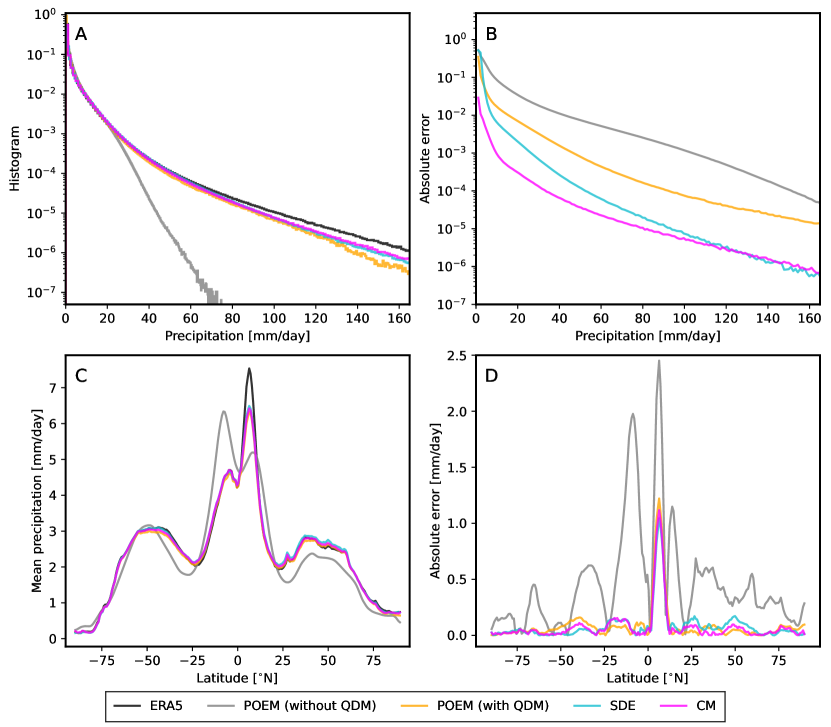
Figure 4: Comparison of global histograms and longitudinal mean precipitation. (A) Global histograms of relative precipitation frequency for the ERA5 reanalysis data (black), POEM simulations without applying the QDM-preprocessing (grey), POEM simulations with QDM (orange), the SDE bridge (cyan), and the CM (magenta). (B) Absolute errors of the histograms in (A) with respect to the ERA5 ground truth. (C) Precipitation averaged over time and longitudes for the same data as in (A). (D) Absolute errors of the latitude profile in (C). Both the SDE and the CM downscaling method are able to further improve upon the QDM-preprocessing in terms of bias correction, most notably for extreme precipitation.

2.3 Quantifying the Sampling Spread

Our generative CM-based downscaling is stochastic, with a one-to-many mapping of a single ESM field to many possible downscaled realizations. It thus naturally yields a probabilistic downscaling, suitable to estimate the associated uncertainties. By selecting a given spatial scale in the ESM to be preserved by the downscaling method, one automatically chooses a related degree of freedom to generate patterns on smaller scales. Given that our CM method is very efficient at inference, we can generate a large ensemble of high-resolution fields that are consistent with the low-resolution ESM input, and compute statistics such as the sampling spread, which can be interpreted as a measure of the inherent uncertainty of the downscaling task.

We compute an ensemble of $10^{3}$ downscaled fields from a single ESM precipitation field (Fig. 5A) and evaluate the mean and standard deviation (Fig. 5D and Fig. 5E). The ensemble mean shows close similarity to the ESM simulation interpolated to the same high-resolution grid. The sample spread shows patterns similar to the mean, although with a smaller magnitude.

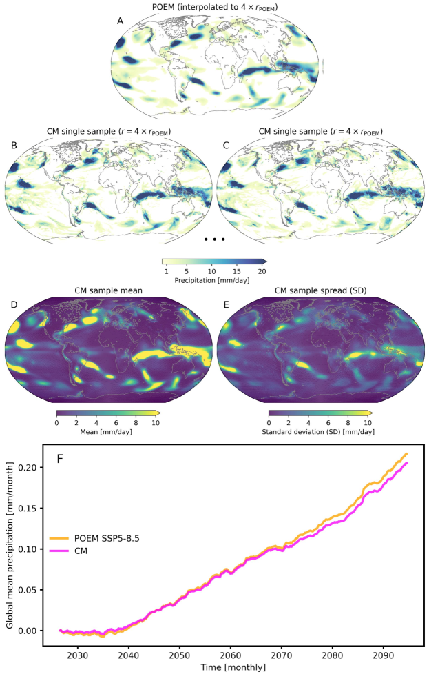
Figure 5: Sampling spread and generalization to unseen climates of the generative probabilistic downscaling process. (A) The ESM field interpolated to the target resolution. (B) and (C) show two different exemplary samples generated by the CM downscaling, preserving large-scale patterns and generating new patterns on smaller scales. (D) The ensemble mean of $10^{3}$ samples with the standard deviation shown in (E). (F) Three-year rolling global mean normalized to the reference year 2020 of the extreme warming scenario SSP5-8.5. The ESM (orange) shows an increase in global mean precipitation over the century in line with the thermodynamic Clausius-Clapeyron relation [Traxl et al., 2021]. The CM downscaling (magenta) is able to preserve the trend with a high degree of accuracy, notably without the addition of any physical constraints in the CM network.

2.4 Future Projections

The efficient nature of our CM approach enables the downscaling of long climate simulations over a century, such as prescribed with the SPP5-8.5 extreme warming scenario from the Coupled Model Intercomparison Project Phase 6 (CMIP6). We find that the downscaling accurately preserves the global precipitation content in the ESM and preserves the non-linear trends of the warming scenario (Fig. 5F). The network thus generalizes to out-of-sample predictions without the need for hard-coding auxiliary physical constraints in the network as, for example, done in [Beucler et al., 2021, Harder et al., 2022, Hess et al., 2022].

3 Discussion

We introduced a generative foundation model for efficient, scale-adaptive, and probabilistic downscaling of ESM precipitation fields. Our approach is based on a novel generative machine learning method that learns a self-consistent approximation of a reversed diffusion process. The CM is able to generate highly realistic global precipitation fields learned from the ERA5 reanalysis, which is employed as ground truth, in a single step. Our framework corrects the representation of extreme events as well as spatial ESM patterns especially at the small spatial scales, which are both crucial for impact assessments. Moreover, spatial biases are also corrected efficiently.

The CM method is up to three orders of magnitude faster than current diffusion models based on SDEs, which need to solve a differential equation iteratively. Crucially, the CM maintains a high degree of controllability to guide the sampling in such a way that spatial patterns larger than a chosen spatial scale in Earth system models are preserved.

Similar to the SDE-based method that [Bischoff and Deck, 2023] apply to idealized fluid dynamics, our CM-based foundation model only needs to be trained once on a given high-resolution observational target dataset. Since we do not condition on ESM input during training, our method can be applied to any ESM without the need for retraining. Combined with the efficient sampling of CMs, our approach is computationally cheap and fast, particularly when processing large ensembles of ESMs, without noticible trade-offs in accuracy.

Our CM-based approach can create highly realistic fields that maintain high correlation levels with the ESM. We find comparable or better results when compared with the much more computationally expensive SDE-based method. The efficient single-step generation of ESM fields will be particularly relevant for processing large datasets, e.g., large ensembles as needed for uncertainty quantification, for simulations with a high temporal resolution, or long-term studies such as those in paleo-climate simulations. Improving the efficiency of current deep learning models is also important from an energy consumption perspective; in this regard our method provides a valuable contribution towards “greener AI” [Schwartz et al., 2019].

When evaluated on a future extreme emission scenario, we find that our generative CM method accurately preserves the trend of the ESM, even for an extreme scenario of greenhouse gas emissions and associated global warming. This is remarkable since many machine learning-based applications to climate dynamics struggle with the out-of-sample problem imposed by our highly non-stationary climate system, when trained on historical data alone. In contrast to previous studies [Beucler et al., 2021, Harder et al., 2022, Hess et al., 2022], to achieve this it is not necessary to add specifically formulated physical constraints to our model. Our unconstrained CM method hence allows for a more natural generalization to unseen climate states, inherently translating non-stationary dynamics from the ESM to the downscaled high-resolution fields.

We showcase our method on uni-variate precipitation simulations, because precipitation is arguably the most difficult to model climate variable. An extension to multi-variate downscaling is a natural extension of our study in future research. In principle, the convolutional CM network can be extended to include further variables as additional channels in a straightforward manner. The consistency scale will then depend on the variable (channel) and might require a separate treatment, which we leave for future research.

Data Availability

The ERA5 reanalysis data is available for download at the Copernicus Climate Change Service (C3S) (https://cds.climate.copernicus.eu/cdsapp#!/dataset/reanalysis-era5-single-levels?tab=overview). The simulation data from the POEM ESM is available at https://doi.org/10.5281/zenodo.4683086.

Code Availability

The Python code for processing and analyzing the data, together with the PyTorch [Paszke et al., 2019] code for training, will be made available on GitHub: https://github.com/p-hss/consistency-climate-downscaling.git.

Competing interests

The authors declare no competing interests.

4 Methods

4.1 Training Data

As a target and ground truth dataset, we use observational precipitation data from the ERA5 reanalysis [Hersbach et al., 2020] provided by the European Center for Medium-Range Weather Forecasting (ECMWF). We bilinearly interpolate the reanalysis data to a resolution of $0.75^{\circ}$ and $0.9375^{\circ}$ in latitude and longitude direction, respectively (i.e. $240\times 384$ grid points), which corresponds to a four times higher resolution compared to the raw Earth system model simulations with $3^{\circ}\times 3.75^{\circ}$ resolution (i.e. $60\times 96)$ grid points).

For the ESM precipitation fields, we use global simulations from the fully coupled Potsdam Earth Model (POEM) [Drüke et al., 2021], which includes model components for the atmosphere, ocean, ice sheets, and dynamic vegetation. Both ESM and reanalysis datasets cover the period from 1940 to 2018, and we split the data into a training set from 1940-1990, a validation set from 1991-2003, and a test set from 2004-2018.

We apply several preprocessing steps to the ESM data. We interpolate the POEM simulations onto the same high-resolution grid as the ground truth ERA5 data for downscaling purposes and model evaluation. A low-pass filter is then applied to remove small-scale artifacts created by the interpolation. Quantile delta mapping (QDM) [Cannon et al., 2015] with 500 quantiles is applied in a standard way to remove distributional biases in the ESM simulation for each grid cell individually. As discussed in section 2.2, the generative downscaling only corrects biases related to a specified spatial scale. Hence, the QDM step ensures a strong reduction of single-cell biases, while the generative downscaling corrects spatial patterns that are physically consistent. Finally, the ESM and ERA5 data are log-transformed, $\tilde{x}=\log(x+\epsilon)-\log(\epsilon)$ with $\epsilon=0.0001$, followed by a normalization approximately into the range [-1, 1].

4.2 Score-based Diffusion Models

The underlying idea of diffusion-based generative models is to learn a reverse diffusion process from a known prior distribution $\mathbf{x}(t=T)\sim p_{T}$, such as a Gaussian distribution, to a target data distribution $\mathbf{x}(t=0)\sim p_{0}$, where $\mathbf{x}\in\mathbb{R}^{d}$ and $d$ is the data dimension, e.g., the number of pixels in an image. Score-based generative diffusion models [Song and Ermon, 2019, Song et al., 2021, Song et al., 2022] generalize probabilistic denoising diffusion models [Ho et al., 2020, Dhariwal and Nichol, 2021] to continuous-time stochastic differential equations (SDEs).

In this framework, the forward diffusion process that incrementally perturbs the data can be described as the solution of the SDE:

$$\mathrm{d}\mathbf{x}=\mu(\mathbf{x},t)\mathrm{d}t+g(t)\mathrm{d}\mathbf{w},$$ (1)

where $\mu(\mathbf{x},t):\mathbb{R}^{d}\rightarrow\mathbb{R}^{d}$ is the drift term, $\mathbf{w}$ denotes a Wiener process and $g(t):\mathbb{R}\rightarrow\mathbb{R}$ is the diffusion coefficient. The reverse SDE used to generate images from noise is given by [Song et al., 2021]

$$\mathrm{d}\mathbf{x}=[\mu(\mathbf{x},t)-g(t)^{2}\nabla_{\mathbf{x}}\log p_{t}(\mathbf{x})]\mathrm{d}\bar{t}+g(t)\mathrm{d}\mathbf{\bar{w}},$$ (2)

with $\bar{t}$ denoting a time reversal and $\nabla_{\mathbf{x}}\log p_{t}(\mathbf{x})$ being the score function of the target distribution. The score function is not analytically tractable, but one can train a score network, $s(\mathbf{x},t;\bm{\phi}):\mathbb{R}^{d}\rightarrow\mathbb{R}^{d}$ to approximate the score function $s(\mathbf{x},t;\bm{\phi})\approx\nabla_{\mathbf{x}}\log p_{t}(\mathbf{x})$, e.g., using denoising score matching [Song et al., 2022] (see SI for details). For sampling, we use the Euler-Maruyama solver to integrate the reverse SDE from $t=T$ to $t=0$ in Eq. 2 with $500$ steps.

4.3 Consistency Models

One major drawback of current diffusion models is that the numerical integration of the differential equation requires around 10-2000 network evaluations, depending on the solver. This makes the generation process computationally inefficient and costly compared to other generative models such as GANs [Goodfellow et al., 2014] or NFs [Dinh et al., 2015, Papamakarios et al., 2021], which can generate images in a single network evaluation. Distillation techniques can reduce the number of integration steps of diffusion models, which often represent a computational bottleneck [Luhman and Luhman, 2021, Zheng et al., 2023].

Consistency models (CMs) can be trained from scratch without distillation and only require a single step to generate a new sample. They have been shown to outperform current distillation techniques [Song et al., 2023]. CMs learn a consistency function, $f(\mathbf{x}(t),t)=\mathbf{x}(t_{\mathrm{min}})$, which is self-consistent, i.e.,

$$f(\mathbf{x}(t),t)=f(\mathbf{x}(t^{\prime}),t^{\prime})\;\forall\;t,t^{\prime}\in[t_{\mathrm{min}},t_{\mathrm{max}}],$$ (3)

where the time interval is here set to $t_{\mathrm{min}}=0.002$ and $t_{\mathrm{max}}=80$. Further, a boundary condition $f(\mathbf{x}(t_{\mathrm{min}}),t_{\mathrm{min}})=\mathbf{x}(t_{\mathrm{min}})$, for $t=t_{\mathrm{min}}$ is imposed. This can be implemented with the parameterization:

$$f(\mathbf{x},t;\bm{\theta})=c_{\mathrm{skip}}(t)\mathbf{x}+c_{\mathrm{out}}(t)F(\mathbf{x},t;\bm{\theta}),$$ (4)

where the coefficients are defined, following [Karras et al., 2022, Song et al., 2023], as

$$c_{\mathrm{skip}}=\frac{\sigma^{2}_{\mathrm{data}}}{((t-t_{\mathrm{min}})^{2}+\sigma^{2}_{\mathrm{data}})},\qquad c_{\mathrm{out}}(t)=\frac{\sigma_{\mathrm{data}}t}{\sqrt{t^{2}+\sigma_{\mathrm{data}^{2}}}}.$$ (5)

The training objective is given by

$$\mathcal{L}\left(\bm{\theta},\bm{\bar{\theta}}\right)=\mathbb{E}_{\mathbf{x},n,t_{n}}\left[d\left(f(\mathbf{x}+t_{n+1}\mathbf{z},t_{n+1};\bm{\theta}),f\left(\mathbf{x}+t_{n}\mathbf{z},t_{n};\bm{\bar{\theta}}\right)\right)\right],$$ (6)

where $\mathbb{E}_{\mathbf{x},n,\mathbf{x}_{t_{n}}}\equiv\mathbb{E}_{\mathbf{x}\sim p_{\mathrm{data}},t_{n}\sim\mathcal{U}(1,N(k)-1),\mathbf{z}\sim\mathcal{N}(\mathbf{0},\mathbf{1})}$, and $N(\cdot)$ increases over training time with a given schedule. With $\bm{\bar{\theta}}$ we denote an exponential moving average (EMA) over the model parameters $\bm{\theta}$, updated with $\bm{\bar{\theta}}=\mathrm{stopgrad}[w(k)\bm{\bar{\theta}}+(1-w(k)\bm{\theta})]$, and a schedule $w(\cdot)$ for the decay rate.

For the distance measure $d(\cdot,\cdot)$, we follow [Song et al., 2023] and use a combination of the learned perceptual image patch similarity (LPIPS) [Zhang et al., 2018] and $l^{1}$ norm:

$$d(\mathbf{x},\mathbf{y})=\mathrm{LPIPS}(\mathbf{x},\mathbf{y})+||\mathbf{x}-\mathbf{y}||_{1}.$$ (7)

4.4 Network Architectures and Training

We use a UNet [Ronneberger et al., 2015, Song et al., 2021] to train both the score and consistency networks, with four down- and upsampling layers. For the four layers, we use convolutions with 128, 128, 256, and 256 channels, respectively, and $3\times 3$ kernels, SiLU activations, group normalization, and an attention layer at the architecture bottleneck.

We train the score network with the ADAM optimizer [Kingma and Ba, 2015] for 200 epochs, with a batch size of $1$, a learning rate of $2e^{-4}$, and an exponential moving average (EMA) over the model weights with a decay rate of 0.999 (see SI for more details).

The CM model is trained for 200 epochs following [Song et al., 2023], with the RADAM optimizer [Liu et al., 2021] and the same batch size, learning rate, and EMA schedule as the score network.

4.5 Scale-Consistent Downscaling

As shown in [Rissanen et al., 2023, Bischoff and Deck, 2023], adding Gaussian noise with a chosen variance to an image (or fluid dynamical snapshot) results in removing spatial patterns up to a specific spatial scale associated with the amount of added noise. The trained generative model can then replace the noise with spatial patterns learned from the training data up to the chosen spatial scale.

In principle, the spatial scale can be chosen depending on the given downscaling task, e.g., ESM resolution or variable. In general, ESM fields are too smooth at high small spatial scales, which presents a key problem for Earth system modelling in general and impact assessments in particular. More specifically, when comparing the frequency distribution of spatial precipitation fields in terms of spatial power spectral densities (PSDs), it can be seen that ESMs lack high-frequency spatial variability, or spatial intermittency, that is a key characteristic of precipitation [Hess et al., 2022]. Hence, a natural choice for the spatial scale to be preserved in the ESM fields is the intersection of the PSDs from the ESM and the ground truth ERA5 [Bischoff and Deck, 2023] (see Fig. 3), i.e., the scale where the ESM fields become too smooth.

For Gaussian noise, the variance as a function of time $t$ can be related to the PSD of a given wavenumber $k$ and the grid size $N$ by [Bischoff and Deck, 2023]

$$\sigma^{2}(t)=N^{2}\mathrm{PSD}(k).$$ (8)

Using Eq. 8, we choose $k^{*}=0.0667$ (see Fig. S1), such that it represents the wavenumber or spatial scale where the PSDs of the ESM and ERA5 precipitation fields intersect. This corresponds to $t^{*}=0.468$ for the CM variance schedule and $t^{*}=0.355$ for the SDE bridge.

The diffusion bridge (DB) [Bischoff and Deck, 2023] starts with the forward SDE in Eq. 1, initialized with a precipitation field from the POEM ESM. The forward SDE is then integrated until $t=t^{*}$. The reverse SDE (Eq. 2), initialized at $t=t^{*}$, then denoises the field again, adding structure from the target ERA5 distribution.

For the CM approach, at inference we apply the “stroke guidance” technique [Meng et al., 2022, Song et al., 2023], where we first sample a noised ESM field $\mathbf{\tilde{x}}^{\mathrm{ESM}}\in\mathbb{R}^{d}$ with variance corresponding to $t^{*}$,

$$\mathbf{\tilde{x}}^{\mathrm{ESM}}\sim\mathcal{N}(\mathbf{x}^{\mathrm{ESM}};\sigma^{2}(t^{*})\mathbf{1}),$$ (9)

which is then denoised in a single step with the CM,

$$\mathbf{\hat{x}}=f(\mathbf{\tilde{x}}^{\mathrm{ESM}},t^{*};\bm{\theta}),$$ (10)

thus highly efficiently generating realistic samples $\mathbf{\hat{x}}$ that preserve spatial patterns of the ESM up to scale $k^{*}$.

References

- [Arjovsky and Bottou, 2017] Arjovsky, M. and Bottou, L. (2017). Towards Principled Methods for Training Generative Adversarial Networks. arXiv:1701.04862 [cs, stat].
- [Beucler et al., 2021] Beucler, T., Pritchard, M., Rasp, S., Ott, J., Baldi, P., and Gentine, P. (2021). Enforcing Analytic Constraints in Neural Networks Emulating Physical Systems. Physical Review Letters, 126(9):98302. arXiv: 1909.00912 Publisher: American Physical Society.
- [Bischoff and Deck, 2023] Bischoff, T. and Deck, K. (2023). Unpaired Downscaling of Fluid Flows with Diffusion Bridges. arXiv:2305.01822 [physics].
- [Cannon et al., 2015] Cannon, A. J., Sobie, S. R., and Murdock, T. Q. (2015). Bias Correction of GCM Precipitation by Quantile Mapping: How Well Do Methods Preserve Changes in Quantiles and Extremes? Journal of Climate, 28(17):6938–6959. Publisher: American Meteorological Society Section: Journal of Climate.
- [Dhariwal and Nichol, 2021] Dhariwal, P. and Nichol, A. (2021). Diffusion Models Beat GANs on Image Synthesis. arXiv:2105.05233 [cs, stat].
- [Dinh et al., 2015] Dinh, L., Krueger, D., and Bengio, Y. (2015). NICE: Non-linear Independent Components Estimation. arXiv:1410.8516 [cs].
- [Drüke et al., 2021] Drüke, M., von Bloh, W., Petri, S., Sakschewski, B., Schaphoff, S., Forkel, M., Huiskamp, W., Feulner, G., and Thonicke, K. (2021). CM2Mc-LPJmL v1.0: biophysical coupling of a process-based dynamic vegetation model with managed land to a general circulation model. Geoscientific Model Development, 14(6):4117–4141. Publisher: Copernicus GmbH.
- [François et al., 2021] François, B., Thao, S., and Vrac, M. (2021). Adjusting spatial dependence of climate model outputs with cycle-consistent adversarial networks. Springer Berlin Heidelberg. Publication Title: Climate Dynamics Issue: 0123456789 ISSN: 14320894.
- [Goodfellow et al., 2014] Goodfellow, I., Pouget-Abadie, J., Mirza, M., Xu, B., Warde-Farley, D., Ozair, S., Courville, A., and Bengio, Y. (2014). Generative Adversarial Nets. In Ghahramani, Z., Welling, M., Cortes, C., Lawrence, N., and Weinberger, K. Q., editors, Advances in Neural Information Processing Systems, volume 27. Curran Associates, Inc.
- [Groenke et al., 2020] Groenke, B., Madaus, L., and Monteleoni, C. (2020). ClimAlign: Unsupervised statistical downscaling of climate variables via normalizing flows. arXiv:2008.04679 [cs, stat].
- [Harder et al., 2022] Harder, P., Yang, Q., Ramesh, V., Sattigeri, P., Hernandez-Garcia, A., Watson, C., Szwarcman, D., and Rolnick, D. (2022). Generating physically-consistent high-resolution climate data with hard-constrained neural networks. arXiv: 2208.05424.
- [Harris et al., 2022] Harris, L., McRae, A. T. T., Chantry, M., Dueben, P. D., and Palmer, T. N. (2022). A Generative Deep Learning Approach to Stochastic Downscaling of Precipitation Forecasts. Journal of Advances in Modeling Earth Systems, 14(10). arXiv:2204.02028 [physics, stat].
- [Hersbach et al., 2020] Hersbach, H., Bell, B., Berrisford, P., Hirahara, S., Horányi, A., Muñoz-Sabater, J., Nicolas, J., Peubey, C., Radu, R., Schepers, D., Simmons, A., Soci, C., Abdalla, S., Abellan, X., Balsamo, G., Bechtold, P., Biavati, G., Bidlot, J., Bonavita, M., De Chiara, G., Dahlgren, P., Dee, D., Diamantakis, M., Dragani, R., Flemming, J., Forbes, R., Fuentes, M., Geer, A., Haimberger, L., Healy, S., Hogan, R. J., Hólm, E., Janisková, M., Keeley, S., Laloyaux, P., Lopez, P., Lupu, C., Radnoti, G., de Rosnay, P., Rozum, I., Vamborg, F., Villaume, S., and Thépaut, J.-N. (2020). The ERA5 global reanalysis. Quarterly Journal of the Royal Meteorological Society, 146(730):1999–2049. _eprint: https://onlinelibrary.wiley.com/doi/pdf/10.1002/qj.3803.
- [Hess et al., 2022] Hess, P., Drüke, M., Petri, S., Strnad, F. M., and Boers, N. (2022). Physically constrained generative adversarial networks for improving precipitation fields from Earth system models. Nature Machine Intelligence, 4(10):828–839. Number: 10 Publisher: Nature Publishing Group.
- [Hess et al., 2023] Hess, P., Lange, S., Schötz, C., and Boers, N. (2023). Deep Learning for Bias-Correcting CMIP6-Class Earth System Models. Earth’s Future, 11(10):e2023EF004002. _eprint: https://onlinelibrary.wiley.com/doi/pdf/10.1029/2023EF004002.
- [Ho et al., 2020] Ho, J., Jain, A., and Abbeel, P. (2020). Denoising Diffusion Probabilistic Models. arXiv:2006.11239 [cs, stat].
- [Karras et al., 2022] Karras, T., Aittala, M., Aila, T., and Laine, S. (2022). Elucidating the Design Space of Diffusion-Based Generative Models. arXiv:2206.00364 [cs, stat].
- [Kingma and Ba, 2015] Kingma, D. P. and Ba, J. L. (2015). Adam: A method for stochastic optimization. 3rd International Conference on Learning Representations, ICLR 2015 - Conference Track Proceedings, pages 1–15. arXiv: 1412.6980.
- [Kotz et al., 2022] Kotz, M., Levermann, A., and Wenz, L. (2022). The effect of rainfall changes on economic production. Nature, 601(7892):223–227. Number: 7892 Publisher: Nature Publishing Group.
- [Liu et al., 2021] Liu, L., Jiang, H., He, P., Chen, W., Liu, X., Gao, J., and Han, J. (2021). On the Variance of the Adaptive Learning Rate and Beyond. arXiv:1908.03265 [cs, stat].
- [Luhman and Luhman, 2021] Luhman, E. and Luhman, T. (2021). Knowledge Distillation in Iterative Generative Models for Improved Sampling Speed. arXiv:2101.02388 [cs].
- [Meng et al., 2022] Meng, C., He, Y., Song, Y., Song, J., Wu, J., Zhu, J.-Y., and Ermon, S. (2022). SDEdit: Guided Image Synthesis and Editing with Stochastic Differential Equations. arXiv:2108.01073 [cs].
- [Pan et al., 2021] Pan, B., Anderson, G. J., Goncalves, A., Lucas, D. D., Bonfils, C. J. W., Lee, J., Tian, Y., and Ma, H.-Y. (2021). Learning to Correct Climate Projection Biases. Journal of Advances in Modeling Earth Systems, 13(10):e2021MS002509. _eprint: https://onlinelibrary.wiley.com/doi/pdf/10.1029/2021MS002509.
- [Papamakarios et al., 2021] Papamakarios, G., Nalisnick, E., Rezende, D. J., Mohamed, S., and Lakshminarayanan, B. (2021). Normalizing flows for probabilistic modeling and inference. The Journal of Machine Learning Research, 22(1):57:2617–57:2680.
- [Paszke et al., 2019] Paszke, A., Gross, S., Massa, F., Lerer, A., Bradbury, J., Chanan, G., Killeen, T., Lin, Z., Gimelshein, N., Antiga, L., Desmaison, A., Kopf, A., Yang, E., DeVito, Z., Raison, M., Tejani, A., Chilamkurthy, S., Steiner, B., Fang, L., Bai, J., and Chintala, S. (2019). PyTorch: An Imperative Style, High-Performance Deep Learning Library. In Advances in Neural Information Processing Systems, volume 32. Curran Associates, Inc.
- [Ravuri et al., 2021] Ravuri, S., Lenc, K., Willson, M., Kangin, D., Lam, R., Mirowski, P., Fitzsimons, M., Athanassiadou, M., Kashem, S., Madge, S., Prudden, R., Mandhane, A., Clark, A., Brock, A., Simonyan, K., Hadsell, R., Robinson, N., Clancy, E., Arribas, A., and Mohamed, S. (2021). Skilful precipitation nowcasting using deep generative models of radar. Nature, 597(7878):672–677. arXiv: 2104.00954 Publisher: Springer US.
- [Rissanen et al., 2023] Rissanen, S., Heinonen, M., and Solin, A. (2023). Generative Modelling With Inverse Heat Dissipation. arXiv:2206.13397 [cs, stat].
- [Ronneberger et al., 2015] Ronneberger, O., Fischer, P., and Brox, T. (2015). U-net: Convolutional networks for biomedical image segmentation. In Lecture Notes in Computer Science (including subseries Lecture Notes in Artificial Intelligence and Lecture Notes in Bioinformatics), volume 9351, pages 234–241. Springer Verlag. arXiv: 1505.04597 ISSN: 16113349.
- [Schneider et al., 2017] Schneider, T., Teixeira, J., Bretherton, C. S., Brient, F., Pressel, K. G., Schär, C., and Siebesma, A. P. (2017). Climate goals and computing the future of clouds. Nature Climate Change, 7(1):3–5. Number: 1 Publisher: Nature Publishing Group.
- [Schwartz et al., 2019] Schwartz, R., Dodge, J., Smith, N. A., and Etzioni, O. (2019). Green AI. arXiv:1907.10597 [cs, stat].
- [Song et al., 2022] Song, J., Meng, C., and Ermon, S. (2022). Denoising Diffusion Implicit Models. arXiv:2010.02502 [cs].
- [Song et al., 2023] Song, Y., Dhariwal, P., Chen, M., and Sutskever, I. (2023). Consistency Models. arXiv:2303.01469 [cs, stat].
- [Song and Ermon, 2019] Song, Y. and Ermon, S. (2019). Generative Modeling by Estimating Gradients of the Data Distribution. In Advances in Neural Information Processing Systems, volume 32. Curran Associates, Inc.
- [Song et al., 2021] Song, Y., Sohl-Dickstein, J., Kingma, D. P., Kumar, A., Ermon, S., and Poole, B. (2021). Score-Based Generative Modeling through Stochastic Differential Equations. arXiv:2011.13456 [cs, stat].
- [Tian and Dong, 2020] Tian, B. and Dong, X. (2020). The Double-ITCZ Bias in CMIP3, CMIP5, and CMIP6 Models Based on Annual Mean Precipitation. Geophysical Research Letters, 47(8):1–11.
- [Traxl et al., 2021] Traxl, D., Boers, N., Rheinwalt, A., and Bookhagen, B. (2021). The role of cyclonic activity in tropical temperature-rainfall scaling. Nature Communications, 12(1):6732. Number: 1 Publisher: Nature Publishing Group.
- [Wan et al., 2023] Wan, Z. Y., Baptista, R., Chen, Y.-f., Anderson, J., Boral, A., Sha, F., and Zepeda-Núñez, L. (2023). Debias Coarsely, Sample Conditionally: Statistical Downscaling through Optimal Transport and Probabilistic Diffusion Models. arXiv:2305.15618 [physics].
- [Zhang et al., 2018] Zhang, R., Isola, P., Efros, A. A., Shechtman, E., and Wang, O. (2018). The Unreasonable Effectiveness of Deep Features as a Perceptual Metric. arXiv:1801.03924 [cs].
- [Zheng et al., 2023] Zheng, H., Nie, W., Vahdat, A., Azizzadenesheli, K., and Anandkumar, A. (2023). Fast Sampling of Diffusion Models via Operator Learning. In Proceedings of the 40th International Conference on Machine Learning, pages 42390–42402. PMLR. ISSN: 2640-3498.
- [Zhu et al., 2017] Zhu, J.-Y., Park, T., Isola, P., and Efros, A. A. (2017). Unpaired Image-To-Image Translation Using Cycle-Consistent Adversarial Networks. In Proceedings of the IEEE International Conference on Computer Vision, pages 2223–2232.