Absence of torsion : Clue from Starobinsky model of gravity
Abstract
One of the surprising aspects of the present Universe, is the absence of any noticeable observable effects of higher-rank antisymmetric tensor fields, such as space-time torsion, in any natural phenomena. Here, we address the possible explanation of torsion, which may often be identified with the field strength tensor of the second rank antisymmetric Kalb-Ramond field. Within the framework of f(R) gravity, we explore the cosmological evolution of the scalar degrees of freedom associated with higher curvature term in a general higher curvature model . We show that while the values of different cosmological parameters follow acceptable values in the framework of standard cosmology at different epochs for different forms of higher curvature gravity (i.e. different values of n ), only for Starobinsky model (n = 2), the Kalb-Ramond field gets naturally suppressed with cosmological evolution. In contrast, for other models (n both positive and negative), despite their agreement with standard cosmology, the scalar field associated with the higher derivative degree of freedom induces an enhancement in the Kalb-Ramond field and thereby contradicts the observation. The result does not change even if we include the Cosmological Constant. Thus, our result reveals that among different models, Starobinsky model successfully explains the suppression of space-time torsion along with a consistent cosmological evolution.
I Introduction
We haven’t observed any overt indications of antisymmetric tensor fields having an impact on anything that occurs naturally, which is a rather startling aspect of our Universe. In this context, the second-rank antisymmetric tensor field, known as the Kalb-Ramond (KR) field [1], has been studied extensively. Such field appears naturally to cancel gauge anomaly in superstring theory[2, 3]. It has also been shown that the KR field has a natural geometric interpretation as space-time torsion in background geometry through an antisymmetric extension of the affine connection[4, 5, 6]. While it is simple to argue that the coupling of the KR field to matter should be , which is the same as the coupling of gravity with matter, based on dimensional considerations, there hasn’t been any experimental signature of the KR field in the observable Universe. As a result, it can be inferred that if such tensor fields exist, they must be greatly suppressed at the current scale of the Universe.
It was shown earlier that the presence of warped extra spatial dimension may lead to suppression of antisymmetric tensor field of various ranks[7, 8, 9, 10, 11]. While any extra-dimensional theory brings in a plethora of other predictions hitherto unobserved, within the domain of 3+ 1 dimensional Einstein gravity , it is hard to explain the reason of the disappearance of torsion from the geometry. As an alternative, in this work, we want to explore a dynamical mechanism of this suppression of the KR field as well as the other higher rank anti-symmetric fields in the light of higher curvature theory. The presence of suitable higher curvature terms in the gravity action is permissible as long as they satisfy diffeomorphic invariance [12, 13, 14, 15, 16]. In this context theories invoked great interest in the context of various cosmological predictions so far unexplained[17, 18, 19, 20, 21, 22, 23, 24, 25, 26, 27, 28]. Higher order terms in the gravity actions in such models are automatically suppressed by Planck scale which explains why at low energy only Einstein’s term dominates over the others. However, at high energy or at the epoch of early universe , the higher curvature term will have significant presence and in this context Starobinsky model [29] has been studied extensively in different context[30, 31, 32, 33, 34, 35]. In this work, we explore whether the dynamical evolution in the presence of higher curvature gravity in 3+1 dimension may lead to a natural geometric suppression of space-time torsion.
In section 2, we present the standard formalism of transformation of an action in gravity including different fields namely Kalb Ramond field, gauge field and spin 1/2 fermion fields to Einstein gravity through a conformal transformation which manifests higher curvature in terms of a scalar degree of freedom along with a potential. This transformation has been extensively discussed in the literature[12, 13, 17]. In section 3, we present the field equations of the transformed action in an isotropic and homogeneous universe. The conformal transformation induces coupling between different matter with the scalar field. And the field equations suitably change to accommodate the conservation of the energy momentum tensors[13, 17]. The coupled nonlinear equations are presented as a set of autonomous system in terms of a new set of dynamical variables. The form of and the potentials generated from this modified gravity are discussed in section 4. Section 5 presents the solutions of the field equations in three different cases - A) or the Starobinsky model, B) or generalised Starobinsky model and C) Both the models with Cosmological constant. Finally, we conclude in section 6.
II Formalism and Conformal Transformation
The action of massless KR field along with spin 1/2 fermion and gauge field in a background f(R) gravity in four dimensions can be written as[36]
| (1) |
where is the field strength of the KR field. The third and fourth terms in the action (1) are the kinetic terms of spin-1/2 fermion fields and the U(1) gauge field respectively. The last two terms represent the interaction of the KR field i.e., torsion with the fermion and the gauge field respectively. These coupling terms are responsible for finding some signatures for the KR field.
III Field Equations in Einstein Frame
Our goal is to explore how the scalar field evolves cosmologically in the Einstein frame in a background FRW space-time in order to understand whether the coupling of the scalar field with other fields suppresses or enhances the interactions as the universe evolves. And to do so, we further rewrite the entire action into two parts - one part consists of the scalar field () in Einstein gravity and the other part contains all other matter fields, namely, fermions, gauge fields, and Kalb Ramond fields which are coupled to the scalar field through the metric . Note that we do not consider any back reaction of these fields on the scalar field.
| (5) | ||||
where is the Lagrangian density of the scalar field and is the Lagrangian density of matter fields. The energy-momentum tensor of the scalar field and matter, respectively is defined as,
| (6) |
Variation of the action (5) with respect to the field gives the dynamical equation for the scalar field
| (7) |
where . Hence
| (8) |
Equation (7) thus appear as
| (9) |
where is the strength of the coupling between the field and matter, which is constant for any form of .
The matter in Einstein frame (6) is considered as perfect fluid .
and are the energy density and pressure of all kinds of matter in the Einstein frame which are related to the energy-momentum tensor of matter in the Jordan frame by .
In the observable universe, we consider the total energy density consist of radiation and matter (baryonic and CDM) i.e., .
Hence the presence of () in equation (9) indicates that the field couples with matter and not with radiation.
Considering the background space-time to be represented by a flat FRW metric in the Einstein frame
| (10) |
the field equations are
| (11) |
| (12) |
where . The conservation equation for matter is
| (13) |
Denoting the energy density of the field and the pressure of the field , one can rewrite equation (12) as
| (14) |
Using the standard thermodynamic relation , one can easily find a relation between and from equation (13)
| (15) |
So the set of dynamical equations to be handled are
| (16) |
| (17) |
| (18) |
| (19) |
where prime denotes the differentiation with respect to . Note that, since interacts with matter , equations (17) and (18) are coupled whereas radiation is separately conserved (19).
In order to solve these coupled nonlinear inhomogeneous equations, we introduce a set of dynamical variables [37, 38, 39]
| (20) |
and rewrite the equations (16-19) in terms of these new variables forming a set of autonomous systems of first-order differential equations
| (21) |
where, . In terms of these new variables, equation (16) takes the form .
IV General class of :
In this work, we consider a very general class of modified gravity , where has a suitable dimension. The Starobinsky model of modified gravity corresponds to i.e., , where . With this general form of , the corresponding potential is
| (22) |
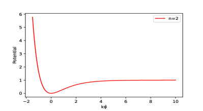
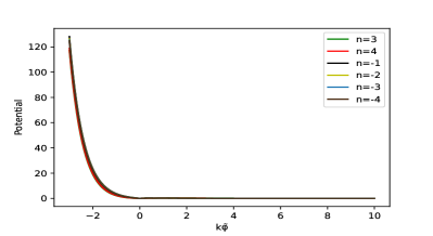
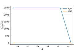
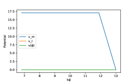
where . The potential becomes zero at , irrespective of . For , the potential is constant when is positive. For negative it increases exponentially. For , the exponential term outside the bracket is the dominating term . For , the power of term within the bracket, i.e, is positive but less than 2 and for , it is positive but less than 1. So, the potential increases sharply for negative and goes to for positive . In fig (1) we present the form of potentials for various values of with .
For the general potential takes a nontrivial form
| (23) |
In terms of the new variables appears as
| (24) |
We use the above form of in the set of autonomous system (21) and solve them numerically with suitable initial conditions, taking different integral values of ranging from -4 to 4. Corresponding to different values of , the expression for changes and hence the set of equations.
V Different cases of
V.1 Case I: , Starobinsky model
For , takes the form , which is the famous Starobinsky model. Substituting the value of in the expression of (24), the equation becomes
| (25) |
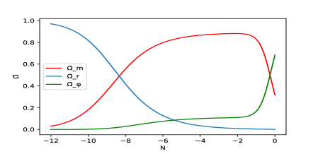
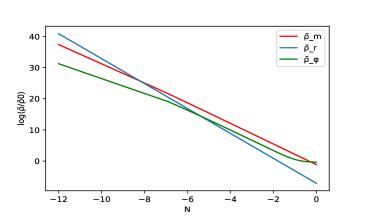
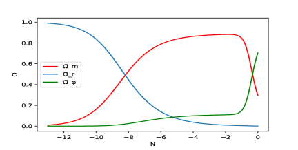
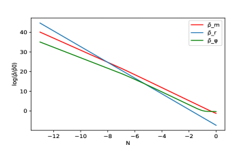
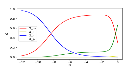
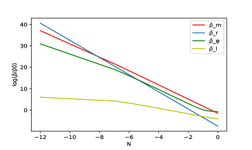
Note that the other equations in (21) remain the same. We solve the above equations numerically, with suitable initial conditions such that radiation-matter equality happens around redshift 3300 and matter in the present universe constitutes approximately 30% of the energy density. On the left in Fig (2), we present different density parameters with respect to and the evolution of the energy densities for all the components are given on the right. The density parameters of different components mimic the behaviours in standard model of cosmology. From both the plots it is evident that the energy density of field never dominates the evolution until recently. Most of the time it scales as matter and becomes constant recently.
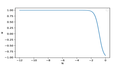
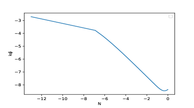
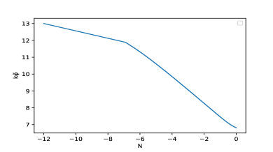
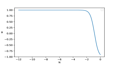
To understand better the evolution and nature of the field we further plot and the equation of state in Fig (3). remains positive along the entire evolution and does not vary much. remains constant for a long period and starts varying late, around and finally approaches at present. So, in the late time the field behaves as dark energy. This behaviour of resembles the equation of state of the thawing quintessence field.
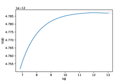
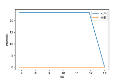
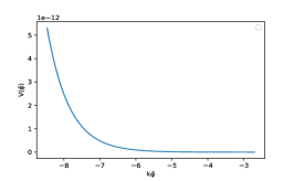
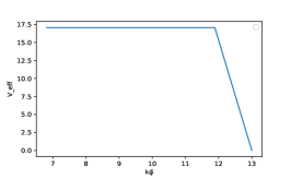
We further investigate the potential responsible for such behaviour of the field and (Fig 4). We find that the field rolls down the potential but does not reach the minima. This brings our attention to the right hand side of the equation (12), which modifies the potential term present in the Klein Gordon equation. Plotting both the terms separately, we realised that the potential arising due to coupling with matter is far more dominant than the potential arising from modified gravity . Hence the effective potential faced by the field is practically the potential due to matter coupling .

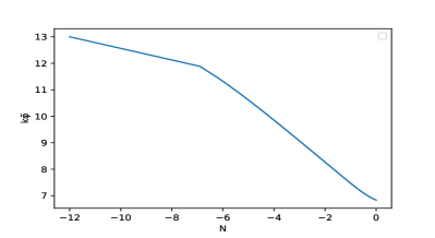
However, remains positive along the entire evolution and does not vary much. Such values of in action (4) ensure that the torsion is heavily suppressed, thereby failing to leave some imprints in the observable universe.
V.2 Case 2: ,
Similarly, we have studied the other cases where takes positive values as well as negative values in the modified gravity form and suitably changed the set of dynamical equations. We have already noticed that for all these cases, the potential form remains the same irrespective of different values of . This hints that for all other cases the results are expected to be same. Hence we present here only one case () as an example. For , the equation becomes
| (26) |
along with the other equations in equation(21). Following similar methods as mentioned above, we solve the equations numerically, with suitable initial conditions to maintain radiation-matter equality around redshift 3300 and . We did a similar analysis of the cosmological parameters as we have done in the case of . Interestingly, the behavior of the density parameters, energy densities and the equation of state almost exactly matches the Starobinsky model over the entire period of evolution. Though the form of the potential of in this case is different from the Starobinsky model, the potential due to coupling dominates, hence the effective potential almost similarly matches the case of .

The equation of state becomes in the recent past, but evolves to lesser negative value at present. Though the energy density of the field is never dominant until recently and scales as matter just like the Starobinsly model, strikingly, the field is negative for the entire period. Such values of in action (4) would imply enhancement and signatures of the torsion field should be present, which is contrary to the observation. For all other values of , we get the same results.

V.3 models with Cosmological Constant
We have also carried out the entire study including the Cosmological Constant along with the other matter components in the observable universe i.e, . Following (9), the field couples with also, apart from matter. So, we change equation (16) to include and equation (17) to incorporate the coupling with . While (18) and (19) remain unchanged as they do not couple with , we have one more coupled equation for ,
| (27) |
| (28) |
| (29) |
To proceed with the analysis we define one more dynamical variable . In terms of all the dynamical variables, the new set of equations to be dealt with looks like
| (30) | ||||
We perform a similar numerical analysis with the new set of equations for the potential given by (22) with different as has been done without . Surprisingly, we found that inclusion of the Cosmological constant does not effect the evolution of different components. Now we have two terms in the right hand side of (28), which together contribute to the effective potential along with . And like the earlier scenario, the coupling term with matter is far more dominant than the potential arising out of modified gravity as well as the coupling with the cosmological constant . In fact in the figure, and are superposed as both are very close to 0. Hence driven mostly by the matter coupling term , the evolution of different components remain similar. The value of the scalar field for different also matches our earlier findings. For , scalar field remains positive throughout, while for other models it remains negative even after inclusion of . Here we present only one case as an example, .

VI Conclusion
In our current universe, we don’t see any signs of antisymmetric tensor fields(torsion) having an impact on natural events, though theoretically, we find that the coupling of KR field to matter is of the order of 1/, equivalent to the coupling of gravity with matter. We explained the suppression of KR field in the light of the higher curvature theory. It has been extensively discussed in literature that modified gravity is equivalent to Einstein gravity along with a scalar field following a potential, which is governed by the form of . Thus, modified gravity when expressed in the Einstein frame, couples with all the other fields (energy-momentum tensors) through the conformal transformation of the metric, apart from radiation. So, the field equations suitably change to accommodate the conservation of the energy momentum tensors. In this work, we have explored how different components like scalar field, radiation and matter evolve in a background isotropic and homogeneous universe represented by FRW metric and the effect of the field on antisymmetric tensor field, particularly Kalb Ramond field.
For this study, we have considered the form of to be , where has suitable dimensions. As shown in fig(1), the shape of the potential for this form is same for all values of , apart from . For , the potential is zero for positive and increases exponentially for . The case, Starobinsky model, is different from the rest, as the potential increases and soon reaches a constant for positive but for negative , the behaviour is the same as other cases. The field equations with different matter and fields in the homogeneous and isotropic background are coupled nonlinear differential equations. We rewrite the equations as a set of autonomous system of first order differential equations to tackle the complexity. Further we solve the autonomous system numerically, with suitable initial conditions such that, following standard model of cosmology, the matter radiation equality occurs around redshift and the matter content is of the total in the present universe.
Though we studied different cases within the range , depending on the behaviour of the potential, we broadly divide them into two categories and . We found the evolution of all components mimic their behaviour in standard model of cosmology and the scalar field is subdominant throughout the evolution of the universe until recently. Further investigation of the equation of state reveals in the late time behaves as a source of dark energy, which resemble the behaviour of thawing quintessence model. Surprisingly we obtained similar behaviours for all of these parameters for both the categories , even though the potentials are different. The reason for such similarity is that the dynamics is dominated by the coupling between matter and , which gives rise to an effective potential. The effective potential exhibit similar nature for different values of and the variation in the values of the parameter in the potential does not lead to any significant change in cosmological evolution.
Most interestingly, even though the different components, namely matter, radiation and scalar field evolve in the similar fashion for different values of , is positive only for and negative for , throughout. The value of depends on the slope of the potential. As discussed earlier, equation (12) reveals that the scalar field rolls down the potential but does not reach the minima due to the coupling with matter which is dominating. For , remains positive as it rolls towards the minima (). Where as, for , can roll only over negative value, as on the positive side the potential is zero. Again this time also, it cannot reach zero due to the coupling. Hence even though both the categories agree with standard model of cosmology, only Starobinsky model , shows the suppression of KR field. For , we obtain the enhancement of KR field instead of the suppression. As there has been no experimental evidence of the footprint of the KR field on the present Universe, so i.e., the Starobinsky model is the only model to support the suppression of the KR field in the gravity where . We have also added cosmological constant as another component. Even though also couples with , the effect is very less with respect to matter- coupling which remains the dominant term. So, the dynamics and our inference regarding the suppression of the KF field remain unchanged.
VII Acknowledgement
Sonej Alam acknowledges the CSIR fellowship provided by Govt. of india under the CSIR-JRF scheme(CSIR NET JUNE 2020). The authors would like to thank Wali Hossain and Anjan A Sen for their invaluable insights and suggestions.
References
- Kalb and Ramond [1974] M. Kalb and P. Ramond, Classical direct interstring action, Phys. Rev. D 9, 2273 (1974).
- Polchinski [1998] J. Polchinski, Contents, in String Theory, Cambridge Monographs on Mathematical Physics (Cambridge University Press, 1998) p. ix–xii.
- Green et al. [2012] M. B. Green, J. H. Schwarz, and E. Witten, Frontmatter, in Superstring Theory: 25th Anniversary Edition, Cambridge Monographs on Mathematical Physics (Cambridge University Press, 2012) p. i–iv.
- Hehl et al. [1976] F. W. Hehl, P. von der Heyde, G. D. Kerlick, and J. M. Nester, General relativity with spin and torsion: Foundations and prospects, Rev. Mod. Phys. 48, 393 (1976).
- de Sabbata and Sivaram [1994] V. de Sabbata and C. Sivaram, Spin and Torsion in Gravitation (WORLD SCIENTIFIC, 1994) https://www.worldscientific.com/doi/pdf/10.1142/2358 .
- Majumdar and Gupta [1999] P. Majumdar and S. S. Gupta, LETTER TO THE EDITOR: Parity-violating gravitational coupling of electromagnetic fields, Classical and Quantum Gravity 16, L89 (1999), arXiv:gr-qc/9906027 [gr-qc] .
- Mukhopadhyaya et al. [2002] B. Mukhopadhyaya, S. Sen, and S. SenGupta, Does a randall-sundrum scenario create the illusion of a torsion-free universe?, Phys. Rev. Lett. 89, 121101 (2002).
- Mukhopadhyaya et al. [2007] B. Mukhopadhyaya, S. Sen, and S. SenGupta, Bulk antisymmetric tensor fields in a randall-sundrum model, Phys. Rev. D 76, 121501 (2007).
- Das et al. [2014] A. Das, B. Mukhopadhyaya, and S. SenGupta, Why has spacetime torsion such negligible effect on the universe?, Phys. Rev. D 90, 107901 (2014).
- Das and SenGupta [2011] A. Das and S. SenGupta, Antisymmetric tensor fields in a generalized Randall-Sundrum scenario, Physics Letters B 698, 311 (2011), arXiv:1010.2076 [hep-th] .
- Lebedev [2002] O. Lebedev, Torsion constraints in the randall-sundrum scenario, Phys. Rev. D 65, 124008 (2002).
- Sotiriou and Faraoni [2010] T. P. Sotiriou and V. Faraoni, theories of gravity, Rev. Mod. Phys. 82, 451 (2010).
- De Felice and Tsujikawa [2010] A. De Felice and S. Tsujikawa, f( R) Theories, Living Reviews in Relativity 13, 3 (2010), arXiv:1002.4928 [gr-qc] .
- Nojiri et al. [2017] S. Nojiri, S. D. Odintsov, and V. K. Oikonomou, Modified gravity theories on a nutshell: Inflation, bounce and late-time evolution, Physics Reports 692, 1 (2017), arXiv:1705.11098 [gr-qc] .
- Nojiri and Odintsov [2007] S. Nojiri and S. D. Odintsov, Introduction to Modified Gravity and Gravitational Alternative for Dark Energy, International Journal of Geometric Methods in Modern Physics 04, 115 (2007), arXiv:hep-th/0601213 [hep-th] .
- Nojiri and Odintsov [2011] S. Nojiri and S. D. Odintsov, Unified cosmic history in modified gravity: From F(R) theory to Lorentz non-invariant models, Physics Reports 505, 59 (2011), arXiv:1011.0544 [gr-qc] .
- Paliathanasis [2016] A. Paliathanasis, f(R)-gravity from Killing tensors, Classical and Quantum Gravity 33, 075012 (2016), arXiv:1512.03239 [gr-qc] .
- Das et al. [2018] A. Das, H. Mukherjee, T. Paul, and S. SenGupta, Radion stabilization in higher curvature warped spacetime, European Physical Journal C 78, 108 (2018), arXiv:1701.01571 [hep-th] .
- Banerjee and Paul [2017] N. Banerjee and T. Paul, Inflationary scenario from higher curvature warped spacetime, arXiv e-prints , arXiv:1706.05964 (2017), arXiv:1706.05964 [hep-th] .
- Bahamonde et al. [2016] S. Bahamonde, S. D. Odintsov, V. K. Oikonomou, and M. Wright, Correspondence of F(R) gravity singularities in Jordan and Einstein frames, Annals of Physics 373, 96 (2016), arXiv:1603.05113 [gr-qc] .
- Chakraborty and SenGupta [2016] S. Chakraborty and S. SenGupta, Solving higher curvature gravity theories, European Physical Journal C 76, 552 (2016), arXiv:1604.05301 [gr-qc] .
- Anand et al. [2015] S. Anand, D. Choudhury, A. A. Sen, and S. SenGupta, Geometric approach to modulus stabilization, Phys. Rev. D 92, 026008 (2015), arXiv:1411.5120 [hep-th] .
- Cognola et al. [2008] G. Cognola, E. Elizalde, S. Nojiri, S. D. Odintsov, L. Sebastiani, and S. Zerbini, Class of viable modified f(R) gravities describing inflation and the onset of accelerated expansion, Phys. Rev. D 77, 046009 (2008), arXiv:0712.4017 [hep-th] .
- Odintsov et al. [2017] S. D. Odintsov, D. Sáez-Chillón Gómez, and G. S. Sharov, Is exponential gravity a viable description for the whole cosmological history?, European Physical Journal C 77, 862 (2017), arXiv:1709.06800 [gr-qc] .
- Linder [2009] E. V. Linder, Exponential gravity, Phys. Rev. D 80, 123528 (2009), arXiv:0905.2962 [astro-ph.CO] .
- Bamba et al. [2010] K. Bamba, C.-Q. Geng, and C.-C. Lee, Cosmological evolution in exponential gravity, JCAP 2010 (8), 021, arXiv:1005.4574 [astro-ph.CO] .
- Capozziello et al. [2006] S. Capozziello, S. Nojiri, and S. D. Odintsov, Dark energy: the equation of state description versus scalar-tensor or modified gravity, Physics Letters B 634, 93 (2006), arXiv:hep-th/0512118 [hep-th] .
- Elizalde et al. [2011] E. Elizalde, S. Nojiri, S. D. Odintsov, L. Sebastiani, and S. Zerbini, Nonsingular exponential gravity: A simple theory for early- and late-time accelerated expansion, Phys. Rev. D 83, 086006 (2011), arXiv:1012.2280 [hep-th] .
- Starobinsky [1980] A. A. Starobinsky, A new type of isotropic cosmological models without singularity, Physics Letters B 91, 99 (1980).
- Starobinsky [1981] A. A. Starobinsky, Nonsingular model of the universe with the quantum gravitational de sitter and its observational consequences, in Second Seminar on Quantum Gravity (1981).
- Starobinskii [1979] A. A. Starobinskii, Spectrum of relict gravitational radiation and the early state of the universe, ZhETF Pisma Redaktsiiu 30, 719 (1979).
- Kofman et al. [1987] L. A. Kofman, V. F. Mukhanov, and D. I. Pogosian, The evolution of inhomogeneities in inflationary models in the theory of gravitation with higher derivatives, Zhurnal Eksperimentalnoi i Teoreticheskoi Fiziki 93, 769 (1987).
- Hwang and Noh [2001] J. c. Hwang and H. Noh, /f(R) gravity theory and CMBR constraints, Physics Letters B 506, 13 (2001), arXiv:astro-ph/0102423 [astro-ph] .
- Elizalde et al. [2019a] E. Elizalde, S. D. Odintsov, T. Paul, and D. S.-C. Gómez, Inflationary universe in F (R ) gravity with antisymmetric tensor fields and their suppression during its evolution, Phys. Rev. D 99, 063506 (2019a), arXiv:1811.02960 [gr-qc] .
- Elizalde et al. [2019b] E. Elizalde, S. D. Odintsov, V. K. Oikonomou, and T. Paul, Logarithmic-corrected R2 gravity inflation in the presence of Kalb-Ramond fields, JCAP 2019 (2), 017, arXiv:1810.07711 [gr-qc] .
- Das et al. [2018] A. Das, T. Paul, and S. SenGupta, Invisibility of antisymmetric tensor fields in the light of gravity, Phys. Rev. D 98, 104002 (2018).
- Hossain and Sen [2012] M. W. Hossain and A. A. Sen, Do observations favour Galileon over quintessence?, Physics Letters B 713, 140 (2012), arXiv:1201.6192 [astro-ph.CO] .
- Brahma and Hossain [2019] S. Brahma and M. W. Hossain, Dark energy beyond quintessence: constraints from the swampland, Journal of High Energy Physics 2019, 70 (2019), arXiv:1902.11014 [hep-th] .
- Ali et al. [2012] A. Ali, R. Gannouji, M. W. Hossain, and M. Sami, Light mass galileons: Cosmological dynamics, mass screening and observational constraints, Physics Letters B 718, 5 (2012), arXiv:1207.3959 [gr-qc] .