Quantum Zeno Monte Carlo for observable measurement

Abstract

The advent of logical quantum processors marks the beginning of the early stages of error-corrected quantum computation. As a bridge between the noisy intermediate scale quantum (NISQ) era and the fault-tolerant quantum computing (FTQC) era, these devices and their successors have the potential to revolutionize the solution of classically challenging problems. An important application of quantum computers is to calculate observables of quantum systems. This problem is crucial for solving quantum many-body and optimization problems. However, due to limited error correction capabilities, this new era are still susceptible to noise, thereby necessitating new quantum algorithms with polynomial complexity as well as noise-resilience. This paper proposes a new noise-resilient and ansatz-free algorithm, called Quantum Zeno Monte Carlo. It utilizes the quantum Zeno effect and Monte Carlo integration for multi-step adiabatic transitions to the target eigenstates. It can efficiently find static as well as dynamic physical properties such as ground state energy, excited state energies, and Green’s function without the use of variational parameters. This algorithm offers a polynomial computational cost and quantum circuit depth that is significantly lower than the quantum phase estimation.

1 The onset of the error-corrected quantum computing era

The quantum computer [1, 2, 3] utilizes quantum algorithms to tackle computationally challenging problems, offering potential solutions to classically hard problems. A significant challenge lies in finding Hamiltonian eigenstates and their physical properties [4], crucial for material design and quantum machine learning implementation. By providing an initial state sufficiently close to the target eigenstate, this problem can be solved within polynomial quantum time [5, 6] with a fully fault-tolerant quantum computer (FTQC) [7, 8]. However, the preceding decades have been marked by the noisy intermediate-scale quantum (NISQ) era [9] rather than the FTQC era. Due to substantial device noise, quantum algorithms for NISQ systems prioritize noise resilience, leading to the dominance of ansatz-based algorithms [10, 11] without provable polynomial complexity.

The emergence of quantum devices with 48 logical qubits [12] marks the start of error-corrected quantum computing. These devices, along with their future advancements, have the potential to showcase quantum advantage, bridging the gap between NISQ and FTQC eras. Early error-corrected quantum computers are expected to handle longer quantum circuits than NISQ devices and execute quantum algorithms with polynomial complexity. However, algorithms designed for the FTQC era may not be suitable for early error-corrected quantum computers, as they still face device noise due to limited error corrections. As a result, developing new quantum algorithms that exhibit polynomial complexity and are resilient to noise shows promise for achieving quantum advantage in early error-corrected quantum computers.

We introduce the quantum Zeno Monte Carlo (QZMC) algorithm. This algorithm is robust against device noise as well as trotter error. Furthermore, this algorithm enables the computation of static as well as dynamic physical properties for quantum systems within polynomial quantum time. We validate its noise resilience by implementing it on IBM’s NISQ devices for small systems. We also demonstrate its polynomial complexity using analytical approach and numerical demonstration on a noiseless quantum computer simulator. Interstingly, the maximum quantum circuit depth required is notably shorter than that of the quantum phase estimation algorithm [13, 14]. (See Supplementary Information for comparison with other methods [15, 16, 17].)

2 Quantum Zeno methods

The Quantum Zeno Monte Carlo algorithm draws inspiration from the quantum Zeno effect [18]. This is the phenomenon that repeated measurements slow down state transitions. We briefly outline this effect: A system varying with a continuous variable $\lambda$ is represented by the state $\ket{\psi_{\lambda}}$. Increasing $\lambda$ to $\lambda+\Delta\lambda$ yields the state $\ket{\psi_{\lambda+\Delta\lambda}}$, which remains $\ket{\psi_{\lambda}}$ with a probability of $|\braket{\psi_{\lambda}}{\psi_{\lambda+\Delta\lambda}}|^{2}$. Because its maximum is at $\Delta\lambda=0$, this probability becomes $1-\mathcal{O}((\Delta\lambda)^{2})$ for sufficiently small $\Delta\lambda$. By dividing $\Delta\lambda$ into $N$ slices and measuring at each interval of $\Delta\lambda/N$, the probability of measuring $\ket{\psi_{\lambda}}$ at every step is $1-\mathcal{O}((\Delta\lambda)^{2}/N)$. Increasing the measurement frequency $N$ ensures the system remains in its initial state $\ket{\psi_{\lambda}}$.

While the original article [18] focused on state freezing through continuous measurements, the principle can also be applied to obtain an energy eigenstate by varying the Hamiltonian for each measurement [19, 20, 21, 22]. Let’s denote our target Hamiltonian as $H$, with its eigenstate as $\ket{\Phi}$. Suppose we have an easily preparable eigenstate $\ket{\Phi_{0}}$ of $H_{0}$ and the state is adiabatically connected to $\ket{\Phi}$. Due to the Van Vleck catastrophe [23, 24], $\ket{\Phi_{0}}$ has very small overlap with $\ket{\Phi}$ in general, potentially requiring a large number of measurements to obtain $\ket{\Phi}$ directly from $\ket{\Phi_{0}}$. Instead, we consider measuring $H_{\alpha}=(1-\alpha/N_{\alpha})H_{0}+(\alpha/N_{\alpha})H$ consecutively for $\alpha=1,\dots,N_{\alpha}$. Utilizing the quantum Zeno principle, we can obtain $\ket{\Phi}$ with very high probability as we increase the number of consecutive measurements $N_{\alpha}$.

3 Quantum Zeno Monte Carlo

The quantum Zeno principle can be implemented using projections, which is equivalent to measurements. Let’s consider $H_{\alpha}=(1-\alpha/N_{\alpha})H_{0}+(\alpha/N_{\alpha})H$, where $\alpha=1,\dots,N_{\alpha}$, and $\ket{\Phi_{0}}$ is the eigenstate of $H_{0}$ that can be readily prepared. For the eigenstate $\ket{\Phi_{\alpha}}$ of $H_{\alpha}$, the operator that projects onto $\ket{\Phi_{\alpha}}$ is represented as $\ket{\Phi_{\alpha}}\bra{\Phi_{\alpha}}$. Then, the consecutive projections $\mathcal{P}_{\alpha}$ applied to $\ket{\Phi_{0}}$ is

$$\ket{\Psi_{\alpha}}=\mathcal{P}_{\alpha}\ket{\Phi_{0}},\quad\mathcal{P}_{\alpha}=\ket{\Phi_{\alpha}}\bra{\Phi_{\alpha}}\dots\ket{\Phi_{1}}\bra{\Phi_{1}},$$ (1)

which is equal to $\ket{\Phi_{\alpha}}$ apart from the normalization. The quantum Zeno principle ensures that $\braket{\Psi_{\alpha}}{\Psi_{\alpha}}=\braket{{\Phi_{0}}}{\mathcal{P}^{\dagger}_{\alpha}\mathcal{P}^{\phantom{\dagger}}_{\alpha}}{{\Phi_{0}}}$ approaches $1$ as $N_{\alpha}\rightarrow\infty$. For the implementation of $\mathcal{P}_{\alpha}$, we use the approximate projection operator defined as

$$P^{\beta}_{H}(E)=\sum_{j}\ket{j}\bra{j}e^{-{\beta^{2}(\mathcal{E}_{j}-E)^{2}}/{2}}=e^{-{\beta^{2}(H-E)^{2}}/{2}},$$ (2)

while $\mathcal{E}_{j}$ and $\ket{j}$ are energy eigenvalues and eigenstates for a Hamiltonian $H$. As $\beta$ increases, Eq. (2) becomes the projection onto the subspace with the energy $E$. Its implementation on the quantum computer can be achieved by using the Fourier expansion [25, 26, 27, 28]

$$P^{\beta}_{H}(E)=\frac{1}{\sqrt{2\pi\beta^{2}}}\int_{-\infty}^{\infty}e^{-\frac{t^{2}}{2\beta^{2}}}e^{-i(H-E)t}dt.$$ (3)

The integrand in Eq. (3) represents the time evolution which can be implemented within a polynomial quantum time [29, 30]. Then, the consecutive projection $\mathcal{P}_{\alpha}$ can be approximated by

$$\mathcal{P}^{\beta}_{\alpha}=P^{\beta}_{H_{\alpha}}(E_{\alpha})\dots P^{\beta}_{H_{1}}(E_{1}),$$ (4)

while $E_{\alpha}$ is the energy eigenvalue of $H_{\alpha}$ corresponds to $\ket{\Phi_{\alpha}}$. By substituting $\mathcal{P}_{\alpha}$ by $\mathcal{P}^{\beta}_{\alpha}$, consecutive projection transforms into a multidimensional integral of consecutive time evolution, which can be computed using the Monte Carlo method [31]. Like recently proposed algorithms [25, 26], our objective is to compute the expectation values $\braket{O}$ of observables rather than the state itself. By using $\ket{\Psi_{\alpha}}$, $\braket{O}_{\alpha}=\braket{\Phi_{\alpha}}{O}{\Phi_{\alpha}}$ can be determined as

$$\braket{O}_{\alpha}=\frac{\braket{\Psi_{\alpha}}{O}{\Psi_{\alpha}}}{\braket{\Psi_{\alpha}}{\Psi_{\alpha}}},$$ (5)

where $\braket{\Psi_{\alpha}}{A}{\Psi_{\alpha}}$ for an arbitrary operator $A$ is computed by the summation of consecutive time evolutions,

$$\frac{1}{N_{\nu}}\sum_{\nu}\braket{\Phi_{0}}{e^{-iK_{1}t_{\nu,2\alpha}}\cdots e^{-iK_{\alpha}t_{\nu,\alpha+1}}Ae^{-iK_{\alpha}t_{\nu,\alpha}}\cdots e^{-iK_{1}t_{\nu,1}}}{{\Phi_{0}}}.$$ (6)

Here, $K_{\alpha^{\prime}}=H_{\alpha^{\prime}}-E_{\alpha^{\prime}}$ for $\alpha^{\prime}=1,\dots,\alpha$ and we use $N_{\nu}$ samples of $\mathbf{t}_{\nu}=[t_{\nu,1}\,\,t_{\nu,2}\,\cdots\,t_{\nu,2\alpha}]^{T}$, where each $t_{\nu,k}$ is drawn from the gaussian distribution with a standard deviation of $\beta$. Consequently, various static and dynamic properties of Hamiltonian eigenstates can be computed using the aforementioned quantum Zeno Monte Carlo (QZMC) method. Figure 1 provides a summary of QZMC. Our approach leverages the concept of the quantum Zeno effect, enabling the construction of unnormalized eigenstate $\ket{\Psi_{\alpha}}$ of $H$ from from easily preparable $\ket{\Phi_{0}}$, as illustrated in Fig. 1a. Then, we compute the observable $\braket{\Phi_{\alpha}}{O}{\Phi_{\alpha}}$ by expanding $\braket{\Psi_{\alpha}}{O}{\Psi_{\alpha}}$ and $\braket{\Psi_{\alpha}}{\Psi_{\alpha}}$ as a summation of the consecutive time evolutions (Fig. 1b).

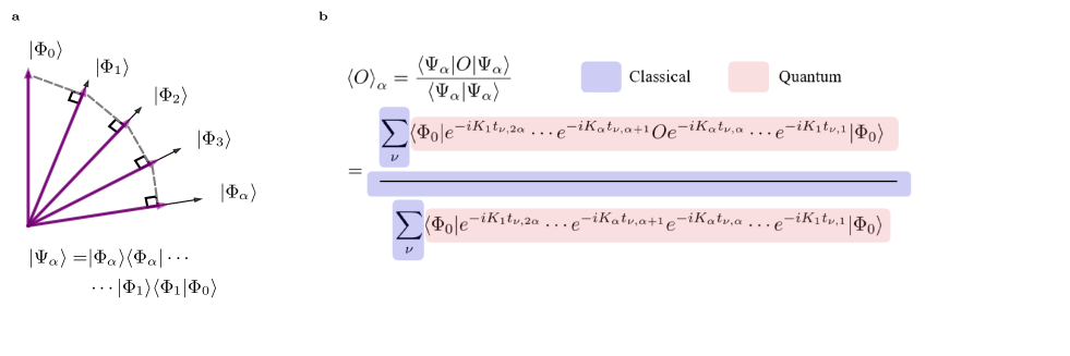
Figure 1:   Overview of the Quantum Zeno Monte Carlo. a depicts the construction of the unnormalized eigenstate $\ket{\Psi_{\alpha}}$ of $H_{\alpha}$ from the eigenstate $\ket{\Phi_{0}}$ of $H_{0}$. Each $\ket{\Phi_{k}}$ represents the normalized eigenstate of $H_{k}$. In b, we present a summary of our Quantum Zeno Monte Carlo for computing the expectation value of an observable ($O$). First, classical computer generates a time vector $\mathbf{t}_{\nu}=[t_{\nu,1}\,\,t_{\nu,2}\,\cdots\,t_{\nu,2\alpha}]^{T}$, where $t_{\nu,k}$ follows Gaussian distribution. Next, quantum computer measure the expectation value with the given time vector. Finally, the sum over $N_{\nu}$ Monte Carlo sampling as well as the division is conducted by using classical conmputer. Here, $K_{\alpha^{\prime}}$ represents $H_{\alpha^{\prime}}-E_{\alpha^{\prime}}$.

The QZMC computation relies on prior knowledge of energy eigenvalues $E_{\alpha}$. Therefore, a practical method for their computation is necessary. Here, we propose the predictor-corrector QZMC method for determining energy eigenvalues. Suppose we know $E_{0},E_{1},\dots E_{\alpha-1}$ and aim to compute $E_{\alpha}$. Similar to the predictor-corrector method used in solving differential equations [32], we begin with a rough estimate of $E_{\alpha}$, termed the predictor. Our predictor for $E_{\alpha}$ is the first-order perturbation approximation [33], given by $E_{\alpha}=E_{\alpha-1}+\langle\Phi_{\alpha-1}|h_{\alpha-1}|\Phi_{\alpha-1}\rangle$, where $h_{\alpha-1}=H_{\alpha}-H_{\alpha-1}$. Subsequently, using the predictor $E_{\alpha}$, we compute a more accurate estimate of $E_{\alpha}$, termed the corrector. We determine the corrector based on the properties of the consecutive projection,

$$E_{\alpha}=E_{\alpha-1}+\frac{\braket{\Psi_{\alpha}\ket{\Phi_{\alpha}}{\bra{\Phi_{\alpha}}}h_{\alpha-1}}{\Psi_{\alpha-1}}}{\|\Psi_{\alpha}\|^{2}}\quad\text{(Corrector)}.$$ (7)

This equation directly computes the energy difference $E_{\alpha}-E_{\alpha-1}$ using QZMC. Compared to estimating the entire energy, this approach enhances robustness against noise by confining noise influences to the energy difference ($E_{\alpha}-E_{\alpha-1}$) alone. Based on this insight, we employed Eq. (7), which can be computed as in Eq. (6) by substituting $\ket{\Phi_{\alpha}}\bra{\Phi_{\alpha}}$ by $P^{\beta}_{H}(E_{\alpha})$. More details of QZMC as well as its extension to compute Green’s function are described in the Supplementary Information.

4 QZMC on NISQ devices

Here, we demonstrate the noise resilience of our algorithm by simulating several systems on NISQ devices. We begin with eigenstates of $H_{0}=H(\lambda=0)$. Then, we create a discrete path from $\lambda=0$ to $\lambda=1$ with $\lambda_{\alpha}=\alpha/N_{\alpha}$, where $N_{\alpha}=10$, and apply the predictor-corrector QZMC for $H_{\alpha}=H(\lambda_{\alpha})$. The first system we consider (Figure 2) is the two-level system with the Hamiltonian. $H(\lambda)=X/2+(2\lambda-1)Z$. Next, we simulate the H₂ molecule (Figure 3a) in the STO-3G basis [34], a typical testbed for quantum algorithms [35, 36]. By constraining the electron number to be 2 and the total spin to be 0 [37, 38], the system can be represented by a 2-qubit Hamiltonian. We calculate the energy spectrum of H₂ as a function of interatomic distance ($R$). Lastly, we consider the $2$-site Hubbard model [39]. The Hubbard dimer (Figure 3b-f) at its half filling and singlet spin configuration can be mapped to a two-qubit Hamiltonian. Energy eigenvalues of the Hubbard dimer are computed by increasing onsite Coulomb interaction($U$).

The two-level system results are displayed in Fig.2. Ground state energy as well as its expectation value of $X$, $Y$ and $Z$ operators are displayed in Fig.2 a and b. Despite device noises in ibmq lima, measured observables match well with exact values (dashed lines). As shown in Fig.2c, computed ground state fidelity, $\mathcal{F}_{\alpha}=|\braket{\Phi_{\alpha}}{\Psi_{\alpha}}|^{2}/\braket{\Psi_{\alpha}}{\Psi_{\alpha}}$, demonstrates accurate projection to the desired state by QZMC.

Interestingly, $\braket{\Psi}{\Psi}$ from the NISQ device, deviates largely from its exact value as well as the one from noiseless simulator, as shown in Fig.2d. This is in a sharp contrast to the agreement in the observables. To understand this discrepancy, we tested the dependence of the measured observables on the device noise magnitude using the qiskit [40] aer simulator. As shown in Figure.2e-f, as the noise level increases, $\braket{\Psi}{\Psi}$ decreases. Simultaneously, the absolute value of $\braket{\Psi}{Z}{\Psi}$ (Fig.2e) also decreases. Surprisingly, these noise-induced errors cancel each other through the ratio of $\braket{\Psi}{\Psi}$ and $\braket{\Psi}{Z}{\Psi}$, so that $\braket{Z}=\braket{\Psi}{Z}{\Psi}/\braket{\Psi}{\Psi}$ (Fig.2f) remains robust against noise. Since quantum circuits for computing the numerator and denominator are nearly identical, division cancels out common noise effects, making the expectation value resilient to noise (See Supplementary Information for quantum circuits [41, 42, 43]).

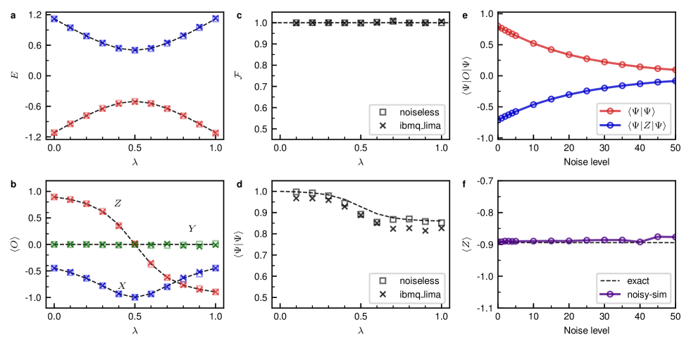
Figure 2:   A two level system. The energy eigenvalues of the ground (red) and the excited state (blue) are plotted in a. In b, we plotted $\braket{X}$ (blue), $\braket{Y}$ (green), and $\braket{Z}$ (red) calculated for the ground states. c and d display the fidelity $\mathcal{F}$ and $\braket{\Psi}{\Psi}$ for the ground state. In a-d, dotted lines represent the exact result, boxes represent QZMC results with a noiseless simulator, and crosses represent results with ibmq lima. We plotted $\braket{\Psi}{\Psi}$, $\braket{\Psi}{Z}{\Psi}$, and $\braket{Z}$ as a function of the noise level in e and f, The calculations for e-f are conducted with the qiskit noisy simulator using the noise model of ibmq lima. In this figure, we used $\beta=5$ and $N_{\nu}=400$.

Figure 3 presents computational results for two-qubit systems: H₂ and the Hubbard dimer. We determined the energy eigenvalues of H₂ within an error of $0.02\,$Ha using ibm lagos. Energy eigenvalues for the Hubbard dimer are calculated within an error of $0.06\,t$ on ibm perth, where $t$ is electron hopping between two hubbard atoms. The influences of device noise are much larger for two-qubit systems compared to one-qubit systems, leading to significant deviations in $\braket{\Psi}{\Psi}$ from exact values, as shown in Figure 3c.

However, as depicted in Figures 3a-b, eigenenergies are accurately reproduced despite large errors in $\braket{\Psi}{\Psi}$. This is partly due to the noise cancellation through division. In addition to the noise cancellation effect demonstrated in Fig. 2 e-f, this noise resilience also rooted in the energy difference estimator Eq. (7). Fig. 3d shows that the formula in Eq. (7) for the estimator results in a smoother line compared to the formula for $\braket{H_{\alpha}}_{\alpha}$. Lastly, we compute the electronic spectral function $A(\omega)$ [44] of the Hubbard dimer with the NISQ device. Figures 3e-f displays $A(\omega)$ at $k=0$ and $k=\pi$, showing good agreements between exact values and measured values.

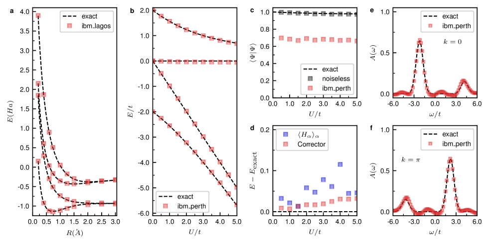
Figure 3:   H₂ and the Hubbard dimer. a plots energy eigenvalues of H₂ in a STO-3G basis as a function of the bond length. Here, we used $\beta=5$ and NISQ device calculation is conducted with ibm lagos. In b-f, we considered the Hubbard dimer. b shows energy eigenvalues as a function of the Coulomb interaction $U$. In c, we compared $\braket{\Psi}{\Psi}$ of the ground state calculated with the NISQ device with exact values and noiseless QZMC results. d compares two energy estimator $\braket{H_{\alpha}}_{\alpha}$ and Eq. (7). The spectral functions for two different crystal momentum $k=0$ (e) and $k=\pi$ (f) are plotted. For the Hubbard dimer, we used $\beta=0.5$ and ibm perth is used. In this figure, we used $N_{\nu}=100$ Monte Carlo samples for each $\alpha$ and and the spectral function is calculated with $300$ Monte Carlo samples.

5 QZMC on large systems

We demomstrate polynomial complexity of our method by applying QZMC to large system with noiseless qsim-cirq [45] quantum computer simulator. We considered the Hubbard model at the half-filling in various sizes. As $H_{0}$, we choose dimer array, featuring easily implementable non-degenerate ground state. We gradually increased the inter-dimer hopping $t_{\textrm{inter}}$ from $0$ to the desired value $t$ as $\alpha$ increased. We explored two geometries, chains and ladders, with periodic boundary conditions, as illustrated in Figure 4a. For each geometry, we computed systems with $6$, $8$, and $10$ sites when $U/t=5$. For QZMC, we used $\beta=3$, with $N_{\alpha}$ equal to the number of sites and $N_{\nu}$ increases as $h_{\alpha}$ increases. For the time evolution, we used the first order Trotterization [29, 46, 47] , adjusting the Trotter steps as system changes. (See Supplementary information for the details on the choice of $N_{\nu}$ and the number of Trotter steps).

Figure 4b illustrates the computed $\braket{\Psi}{\Psi}$ for the $2\times 5$ Hubbard model. Due to errors in the Trotter time evolution, the calculated $\braket{\Psi}{\Psi}$ significantly deviates from exact values. However, the ground state energy remains robust against Trotter errors due to the error cancellation through division, again. This robustness is comparable to its resilience against device noises, as demonstrated in Figure 4c. The figure shows that QZMC accurately reproduces the exact ground state energy across various configurations, from $6$ to $10$ sites, in both chain and ladder arrangements. Finally, we computed the local spectral function for Hubbard models and they are shown in in Fig. 4d-g. Our results matches exact ones, accurately reproducing the positions and widths of every peak in the spectral functions.

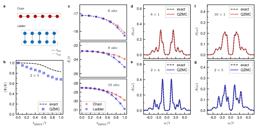
Figure 4:   The Hubbard model in various sizes. a shows two geometries we considered. where colord circles denote sites, solid lines indicate intra-dimer hopping $t_{\textrm{intra}}$, and dotted lines represent inter-dimer hopping $t_{\textrm{inter}}$. b displays $\braket{\Psi}{\Psi}$ for the $2\times 5$ Hubbard model as a function of $t_{\textrm{inter}}$,while c presents ground state energy eigenvalues computed from QZMC. In each subplot of c, red squares denote energies for $6\times 1$, $8\times 1$, and $10\times 1$ models with QZMC, with red dotted lines indicating corersponding exact values. Blue squares and lines represent the same values for $2\times 3$, $2\times 4$, and $2\times 5$ cases. d-g depict the local spectral function for the Hubbard models.

6 Computational complexity

We analyzed the theoretical computational complexity of our method. To facilitate analysis, we adopt a uniform discretization approach, represented by $H_{\alpha}=H_{0}+(\alpha/N_{\alpha})H^{\prime}$ and focus solely on energy estimation complexity. The complexity of other observable measurement can be derived similarly (See Supplementary Information). Let’s first examine the computational complexity of $N_{\nu}$. Our energy difference estimation in Eq. (7) involves a Monte Carlo summation of $\braket{\Phi_{0}}{U_{1}H^{\prime}U_{2}}{\Phi_{0}}$, where $U_{1}$ and $U_{2}$ denote consecutive time evolutions. Since time evolution is unitary, each term in the summation is bounded by $\|H^{\prime}\|$, resulting in a Monte Carlo error $\epsilon$ bouned by $\|H^{\prime}\|/\sqrt{N_{\nu}}$. Hence, the appropriate number of Monte Carlo samples $N_{\nu}$ is proportional to $\|H^{\prime}\|^{2}/\epsilon^{2}$. In most cases, $H^{\prime}$ can be represented as the sum of a polynomial number of Pauli strings [48], which gives $\mathcal{O}(\operatorname{poly}(n))$ upperbound of $\|H^{\prime}\|$. Here $n$ is the number of qubits. Therefore, we can state that $N_{\nu}$ is $\mathcal{O}(\operatorname{poly}(n))/\epsilon^{2}$. Next, let’s consider $N_{\alpha}$ which determines the total number of consecutive time evolutions. According to perturbation theory [33], each projection degrades the norm by about $(\Delta\lambda)^{2}\|H^{\prime}\|^{2}/\Delta^{2}_{g}$. Therefore, for a finite norm, we must have $N_{\alpha}\propto\|H^{\prime}\|^{2}/\Delta^{2}_{g}$. Lastly, let’s determine $\beta$, the width of each projection. For each projection, perturbative analysis shows that a projection error is proportional to $\exp(-\beta^{2}\Delta_{g}^{2}/2)\|H^{\prime}\|/\Delta_{g}$. To ensure this quantity is smaller than error $\epsilon$, $\beta$ must be proportional to $\Delta^{-1}_{g}\sqrt{\operatorname{log}({\|H^{\prime}\|/(\epsilon\Delta_{g})})}$. Since the projection error is relative to the quantity of interest, the energy calculation by using Eq. (7) would have absoulte error $\epsilon$ if $\beta$ is proportional to $\Delta^{-1}_{g}\sqrt{\operatorname{log}({\|H^{\prime}\|^{2}/(\epsilon\Delta_{g})})}$. Because each of time evolution falls within the complexity class BQP (bounded-error quantum polynomial time) [49], we can conclude that QZMC provides energy eigenvalues and various physical properties within a polynomial quantum time, as long as the energy gap $\Delta_{g}$ is finite.

7 Conclusion

In this work, we introduced the quantum Zeno Monte Carlo (QZMC) for the emerging stepping stone era of quantum computing [12]. This method computes static and dynamical observables of quantum systems within a polynomial quantum time. Leveraging the Quantum Zeno effect, we progressively approach the unknown eigenstate from the readily solvable Hamiltonian’s eigenstate. This aspect distinguishes our method from other methods for phase estimations, which necessitate an initial state with significant overlap with the desired eigenstate [5, 6, 15, 26, 17, 27, 50]. Preparing a state with substantial overlap with an eigenstate of an easily solvable Hamiltonian is much simpler than preparing an initial state with non-trivial overlap with the unknown eigenstate, making our algorithm highly practical compared to other methods. Another characteristic of the algorithm is its computation of eigenstate properties by dividing the properties of the unnormalized eigenstate by its norm squared (Eq. 5). We demonstrated that this approach effectively cancels out noise effects in both the denominator and the numerator, rendering the method resilient to device noise as well as Trotter error. This resilience arises from the similar noise levels experienced by both the denominator and the numerator of observable expectation value, leading us to conclude that our approach is well-suited for homogeneous parallel quantum computing.

8 Acknowledgment

We are greatful to Lin Lin for discussions with S.C. This research was supported by Quantum Simulator Development Project for Materials Innovation through the National Research Foundation of Korea (NRF) funded by the Korean government (Ministry of Science and ICT(MSIT))(No. NRF-2023M3K5A1094813). For one and two qubit simulations, we acknowledge the use of IBM Quantum services for this work and to advanced services provided by the IBM Quantum Researchers Program. The views expressed are those of the authors, and do not reflect the official policy or position of IBM or the IBM Quantum team. For larger system calculation, we used resources of the Center for Advanced Computation at Korea Institute for Advanced Study and the National Energy Research Scientific Computing Center (NERSC), a U.S. Department of Energy Office of Science User Facility operated under Contract No. DE-AC02-05CH11231. SC was supported by a KIAS Individual Grant (CG090601) at Korea Institute for Advanced Study. M.H. is supported by a KIAS Individual Grant (No. CG091301) at Korea Institute for Advanced Study.

9 Author contributions

M.H. conceived the original idea. M.H. and S.C. developed the idea into algorithms. M.H implemented and performed classical as well as quantum computer calculation. M.H. established the analytical proof of the computational complexity. All authors contributed to the writing of the manuscript.

10 Competing interests

The authors declare no competing interests.

References

- \bibcommenthead
- [1] Benioff, P. The computer as a physical system: A microscopic quantum mechanical hamiltonian model of computers as represented by turing machines. J. Stat. Phys. 22, 563–591 (1980).
- [2] Feynman, R. P. Simulating physics with computers. Int. J. Theor. Phys. 21 (1982).
- [3] Nielsen, M. A. & Chuang, I. L. Quantum computation and quantum information (Cambridge university press, 2010).
- [4] Shen, Y. et al. Estimating eigenenergies from quantum dynamics: A unified noise-resilient measurement-driven approach. Preprint at https://arxiv.org/abs/2306.01858 (2023).
- [5] Kitaev, A. Y. Quantum measurements and the abelian stabilizer problem. Preprint at https://arxiv.org/abs/quant-ph/9511026 (1995).
- [6] Abrams, D. S. & Lloyd, S. Quantum algorithm providing exponential speed increase for finding eigenvalues and eigenvectors. Phys. Rev. Lett. 83, 5162 (1999).
- [7] Shor, P. W. Fault-tolerant quantum computation in Proc. 37th Conference on Foundations of Computer Science 56–65 (IEEE, 1996).
- [8] Gottesman, D. Theory of fault-tolerant quantum computation. Phy. Rev. A 57, 127 (1998).
- [9] Preskill, J. Quantum Computing in the NISQ era and beyond. Quantum 2, 79 (2018).
- [10] Peruzzo, A. et al. A variational eigenvalue solver on a photonic quantum processor. Nat. Commun 5, 4213 (2014).
- [11] McClean, J. R., Romero, J., Babbush, R. & Aspuru-Guzik, A. The theory of variational hybrid quantum-classical algorithms. New J. Phys. 18, 023023 (2016).
- [12] Bluvstein, D. et al. Logical quantum processor based on reconfigurable atom arrays. Nature 626, 58–65 (2024).
- [13] Berry, D. W. et al. How to perform the most accurate possible phase measurements. Phys. Rev. A 80, 052114 (2009).
- [14] Higgins, B. L., Berry, D. W., Bartlett, S. D., Wiseman, H. M. & Pryde, G. J. Entanglement-free heisenberg-limited phase estimation. Nature 450, 393–396 (2007).
- [15] Lin, L. & Tong, Y. Heisenberg-limited ground-state energy estimation for early fault-tolerant quantum computers. PRX Quantum 3, 010318 (2022).
- [16] Somma, R. D. Quantum eigenvalue estimation via time series analysis. New J. Phys. 21, 123025 (2019).
- [17] Ding, Z. & Lin, L. Even shorter quantum circuit for phase estimation on early fault-tolerant quantum computers with applications to ground-state energy estimation. PRX Quantum 4, 020331 (2023).
- [18] Misra, B. & Sudarshan, E. G. The zeno’s paradox in quantum theory. J. Math. Phys. 18, 756–763 (1977).
- [19] Somma, R. D., Boixo, S., Barnum, H. & Knill, E. Quantum simulations of classical annealing processes. Phys. Rev. Lett. 101, 130504 (2008).
- [20] Poulin, D. & Wocjan, P. Preparing ground states of quantum many-body systems on a quantum computer. Phys. Rev. Lett. 102, 130503 (2009).
- [21] Boixo, S., Knill, E., Somma, R. D. et al. Eigenpath traversal by phase randomization. Quantum Inf. Comput. 9, 833–855 (2009).
- [22] Lin, L. & Tong, Y. Optimal polynomial based quantum eigenstate filtering with application to solving quantum linear systems. Quantum 4, 361 (2020).
- [23] Van Vleck, J. H. Nonorthogonality and ferromagnetism. Phys. Rev. 49, 232–240 (1936).
- [24] Kohn, W. Nobel lecture: Electronic structure of matter—wave functions and density functionals. Rev. Mod. Phys. 71, 1253–1266 (1999).
- [25] Zeng, P., Sun, J. & Yuan, X. Universal quantum algorithmic cooling on a quantum computer. Preprint at https://arxiv.org/abs/2109.15304 (2021).
- [26] Huo, M. & Li, Y. Error-resilient Monte Carlo quantum simulation of imaginary time. Quantum 7, 916 (2023).
- [27] Wang, G., França, D. S., Zhang, R., Zhu, S. & Johnson, P. D. Quantum algorithm for ground state energy estimation using circuit depth with exponentially improved dependence on precision. Quantum 7, 1167 (2023).
- [28] Sun, J., Vilchez-Estevez, L., Vedral, V., Boothroyd, A. T. & Kim, M. Probing spectral features of quantum many-body systems with quantum simulators. Preprint at https://arxiv.org/abs/2305.07649 (2023).
- [29] Lloyd, S. Universal quantum simulators. Science 273, 1073–1078 (1996).
- [30] Zalka, C. Simulating quantum systems on a quantum computer. Proceedings of the Royal Society of London. Series A: Mathematical, Physical and Engineering Sciences 454, 313–322 (1998).
- [31] Kroese, D. P., Taimre, T. & Botev, Z. I. Handbook of Monte Carlo Methods (John Wiley & Sons, 2011).
- [32] Heath, M. T. Scientific computing: an introductory survey, revised second edition (SIAM, 2018).
- [33] Landau, L. D. & Lifshitz, E. M. Quantum mechanics: non-relativistic theory Vol. 3 (Elsevier, 2013).
- [34] Stewart, R. F. Small gaussian expansions of slater-type orbitals. J. Chem. Phys. 52, 431–438 (1970).
- [35] O’Malley, P. J. J. et al. Scalable quantum simulation of molecular energies. Phys. Rev. X 6, 031007 (2016).
- [36] Motta, M. et al. Determining eigenstates and thermal states on a quantum computer using quantum imaginary time evolution. Nat. Phys. 16, 205–210 (2020).
- [37] Seeley, J. T., Richard, M. J. & Love, P. J. The bravyi-kitaev transformation for quantum computation of electronic structure. J. Chem. Phys. 137 (2012).
- [38] Steudtner, M. & Wehner, S. Fermion-to-qubit mappings with varying resource requirements for quantum simulation. New J. Phys. 20, 063010 (2018).
- [39] Hubbard, J. & Flowers, B. H. Electron correlations in narrow energy bands. Proc. R. Soc. London, Ser. A 276, 238–257 (1963).
- [40] https://www.ibm.com/quantum/qiskit.
- [41] Shende, V. V., Markov, I. L. & Bullock, S. S. Minimal universal two-qubit controlled-not-based circuits. Phys. Rev. A 69, 062321 (2004).
- [42] Shende, V., Bullock, S. & Markov, I. Synthesis of quantum-logic circuits. IEEE Transactions on Computer-Aided Design of Integrated Circuits and Systems 25, 1000–1010 (2006).
- [43] Cross, A. W., Bishop, L. S., Sheldon, S., Nation, P. D. & Gambetta, J. M. Validating quantum computers using randomized model circuits. Phys. Rev. A 100, 032328 (2019).
- [44] Negele, J. W. & Orland, H. Quantum many-particle systems Advanced book classics (Westview, Boulder, CO, 1988).
- [45] https://quantumai.google/qsim.
- [46] Trotter, H. F. On the product of semi-groups of operators. Proc. Am. Math. Soc. 10, 545–551 (1959).
- [47] Layden, D. First-order trotter error from a second-order perspective. Phys. Rev. Lett. 128, 210501 (2022).
- [48] Tilly, J. et al. The variational quantum eigensolver: A review of methods and best practices. Phys. Rep. 986, 1–128 (2022).
- [49] Watrous, J. Quantum computational complexity. Preprint at https://arxiv.org/abs/0804.3401 (2008).
- [50] Ni, H., Li, H. & Ying, L. On low-depth algorithms for quantum phase estimation. Quantum 7, 1165 (2023).