Abstract

The learning to defer (L2D) framework allows autonomous systems to be safe and robust by allocating difficult decisions to a human expert. All existing work on L2D assumes that each expert is well-identified, and if any expert were to change, the system should be re-trained. In this work, we alleviate this constraint, formulating an L2D system that can cope with never-before-seen experts at test-time. We accomplish this by using meta-learning, considering both optimization- and model-based variants. Given a small context set to characterize the currently available expert, our framework can quickly adapt its deferral policy. For the model-based approach, we employ an attention mechanism that is able to look for points in the context set that are similar to a given test point, leading to an even more precise assessment of the expert’s abilities. In the experiments, we validate our methods on image recognition, traffic sign detection, and skin lesion diagnosis benchmarks.

1 INTRODUCTION

Hybrid intelligent (HI) systems (Kamar, 2016; Dellermann et al., 2019; Akata et al., 2020) assume some form of on-going collaboration between humans and machines. While this can take many forms, our work focuses on the paradigm of learning to defer (L2D) (Madras et al., 2018): HI systems that can defer to a human upon facing challenging or high-risk decisions. An instructive example is that of automated medicine. Given patient data, the HI system can either make a diagnosis—if it is confident in its prediction—or call in a human doctor to take the case.

Current L2D systems are trained so that the model is customized to one (Mozannar and Sontag, 2020) or more (Verma et al., 2023) specific humans. If the experts’ behavior changes from training- to test-time, the system will break, mis-allocating instances to the human when the machine would perform better or vice versa. An extreme form of this distribution shift is when the expert’s identity completely changes. Returning to the medical setting, this means that when one doctor leaves duty and another takes her place, an entirely new L2D system must be brought online. Similarly, when a new doctor joins the staff, a new L2D system must be trained from scratch (although one can imagine ways to incorporate pre-trained models or existing data).

In this paper, we develop learning to defer to a population: an L2D system that can accurately defer to humans whose predictions were not observed during training. To achieve this, our L2D system is not customized to individuals but rather a population. At test time, we assume that an expert will be drawn from this population, and the L2D system needs to make appropriate deferral decisions despite some uncertainty in how this specific expert will behave. We develop surrogate loss functions for this setting, assuming we have access to similarly-sampled experts to train from, and show that they are consistent.

For a general implementation, we propose meta-learning (Schmidhuber, 1987; Thrun, 1998) on a small context set that is representative of the expert’s abilities. We consider two approaches: one is to fine-tune a model that represents a typical expert, and the other is to encode the context set with a deep-sets architecture (Zaheer et al., 2017). We perform experiments on image recognition, traffic sign detection, and skin lesion diagnosis tasks, showing that our models are able to perform well even as expert variability increases.

2 BACKGROUND

We begin by reviewing the L2D framework for both single (Mozannar and Sontag, 2020) and multiple (Verma et al., 2023) experts. For the whole of this paper, we consider only multi-class classification, but all methods can be straightforwardly extended to other data types, such as real-valued regression (Zaoui et al., 2020).

2.1 Single-Expert Setting

Data & Models

We first define the data for multiclass L2D with one expert. Let $\mathcal{X}$ denote the feature space, and let $\mathcal{Y}$ denote the label space, a categorical encoding of multiple ($K$) classes. ${\mathbf{x}}_{n}\in\mathcal{X}$ denotes a feature vector, and ${\textnormal{y}}_{n}\in\mathcal{Y}$ denotes the associated class defined by $\mathcal{Y}$ (1 of $K$). In order to model the expert’s abilities, L2D assumes that we have access to (human) expert demonstrations. Denote the expert’s prediction space as $\mathcal{M}$ = $\mathcal{Y}$, and let the demonstrations be denoted ${\textnormal{m}}_{n}\in\mathcal{M}$ for the associated features ${\mathbf{x}}_{n}$. The $N$-element training sample is then $\mathcal{D}=\{{\bm{x}}_{n},y_{n},m_{n}\}_{n=1}^{N}$. As for model specification, the L2D framework requires two sub-models: a classifier and a rejector (Cortes et al., 2016b, a). Denote the classifier as $h:\mathcal{X}\rightarrow\mathcal{Y}$ and the rejector as $r:\mathcal{X}\rightarrow\{0,1\}$. The rejector can be interpreted as a meta-classifier, determining which inputs are appropriate to pass to $h({\mathbf{x}})$. When $r({\mathbf{x}})=0$, the classifier makes the decision, and when $r({\mathbf{x}})=1$, the classifier abstains and defers the decision to the human.

Learning

The learning problem requires fitting both the rejector and classifier. When the classifier makes the prediction, then the system incurs a loss of zero (correct) or one (incorrect). When the human makes the prediction (i.e. $r({\bm{x}})=1$), then the human also incurs the same 0-1 loss. Using the rejector to combine these losses, we have the overall classifier-rejector loss:

$$\begin{split}&L_{0-1}(h,r)=\\ &\ \ \mathbb{E}_{{\mathbf{x}},{\textnormal{y}},{\textnormal{m}}}\left[(1-r({\mathbf{x}}))\ \mathbb{I}[h({\mathbf{x}})\neq{\textnormal{y}}]\ +\ r({\mathbf{x}})\ \mathbb{I}[{\textnormal{m}}\neq{\textnormal{y}}]\right]\end{split}$$ (1)

where $\mathbb{I}$ denotes an indicator function that checks if the prediction and label are equal. Upon minimization, the resulting Bayes optimal classifier and rejector satisfy:

$$\begin{split}h^{*}({\bm{x}})&=\operatorname*{arg\,max}_{y\in\mathcal{Y}}\ \mathbb{P}({\textnormal{y}}=y|{\bm{x}}),\\ r^{*}({\bm{x}})&=\mathbb{I}\left[\mathbb{P}({\textnormal{m}}={\textnormal{y}}|{\bm{x}})\geq\max_{y\in\mathcal{Y}}\mathbb{P}({\textnormal{y}}=y|{\bm{x}})\right],\end{split}$$ (2)

where $\mathbb{P}({\textnormal{y}}|{\bm{x}})$ is the probability of the label under the data generating process, and $\mathbb{P}({\textnormal{m}}={\textnormal{y}}|{\bm{x}})$ is the probability that the expert is correct. The expert likely will have knowledge not available to the classifier, and this assumption allows the expert to possibly outperform the Bayes optimal classifier.

Softmax Surrogate

A consistent surrogate loss for the above $L_{0-1}$ loss can be derived following Mozannar and Sontag (2020)’s formulation. First let the classifier and rejector be unified via an augmented label space that includes the rejection option: $\mathcal{Y}^{\bot}=\mathcal{Y}\cup\{\bot\}$, where $\bot$ denotes the rejection option. Secondly, let $g_{k}:\mathcal{X}\mapsto\mathbb{R}$ for $k\in[1,K]$ where $k$ denotes the class index, and let $g_{\bot}:\mathcal{X}\mapsto\mathbb{R}$ denote the rejection ($\bot$) option. These $K+1$ functions can be combined using a loss that resembles the cross-entropy loss for a softmax parameterization:

$$\begin{split}{\upphi}_{\text{SM}}(g_{1}&,\ldots,g_{K},g_{\bot};{\bm{x}},y,m)=\\ &-\log\left(\frac{\exp\{g_{y}({\bm{x}})\}}{\sum_{y^{\prime}\in\mathcal{Y}^{\bot}}\exp\{g_{y^{\prime}}({\bm{x}})\}}\right)\\ &-\mathbb{I}[m=y]\ \log\left(\frac{\exp\{g_{\bot}({\bm{x}})\}}{\sum_{y^{\prime}\in\mathcal{Y}^{\bot}}\exp\{g_{y^{\prime}}({\bm{x}})\}}\right).\end{split}$$ (3)

The intuition is that the first term maximizes the function $g_{k}$ associated with the true label. The second term then maximizes the rejection function $g_{\bot}$ but only if the expert’s prediction is correct. At test time, the classifier is obtained by taking the maximum over $k\in[1,K]$: $\hat{y}=h({\bm{x}})=\operatorname*{arg\,max}_{k\in[1,K]}g_{k}({\bm{x}})$. The rejection function is similarly formulated as $r({\bm{x}})=\mathbb{I}[g_{\bot}({\bm{x}})\geq\max_{k}g_{k}({\bm{x}})]$. The minimizers $g^{*}_{1},\ldots,g^{*}_{K},g^{*}_{\bot}$ of ${\upphi}_{\text{SM}}$ also uniquely minimize $L_{0-1}(h,r)$, the $0-1$ loss from Equation 1 (Mozannar and Sontag, 2020). Verma and Nalisnick (2022) showed that using a one-vs-all parameterization and an analogous loss function is also a consistent surrogate and better estimates the expert’s probability of being correct.

2.2 Multi-Expert Setting

Data & Model

Now let there be $J$ experts, each having a prediction space denoted $\mathcal{M}_{j}$ = $\mathcal{Y}$ $\ \forall j$. Analogously to above, the expert demonstrations are denoted ${\textnormal{m}}_{n,j}\in\mathcal{M}_{j}$ for the associated features ${\mathbf{x}}_{n}$. The combined $N$-element training sample then includes the feature vector, label, and all expert predictions: $\mathcal{D}=\{{\bm{x}}_{n},y_{n},m_{n,1},\ldots,m_{n,J}\}_{n=1}^{N}$. In single-expert L2D, the rejector makes a binary decision—to defer or not—but in multi-expert L2D, the rejector also chooses to which expert to defer. In turn, define the multi-expert rejector as $r:\mathcal{X}\rightarrow\{0,1,\ldots,J\}$. When $r({\mathbf{x}})=0$, the classifier makes the decision, and when $r({\mathbf{x}})=j$, the classifier abstains and the $j$th expert makes the prediction. The classifier sub-model ($h$) is identical to the single-expert case.

Learning

Again the learning objective is to apply the $0-1$ loss to each decision maker:

$$\begin{split}&L_{0-1}(h,r)=\mathbb{E}_{{\mathbf{x}},{\textnormal{y}},\{{\textnormal{m}}_{j}\}_{j=1}^{J}}\Bigg{[}\mathbb{I}[r({\mathbf{x}})=0]\ \mathbb{I}[h({\mathbf{x}})\neq{\textnormal{y}}]\\ &\ \ \ \ \ \ \ \ \ \ \ \ \ \ \ \ \ \ \ \ \ \ \ \ \ \ +\ \sum_{j=1}^{J}\mathbb{I}[r({\mathbf{x}})=j]\ \mathbb{I}[{\textnormal{m}}_{j}\neq{\textnormal{y}}]\Bigg{]}\end{split}$$

The Bayes optimal classifier is the same as in the single-expert setting (Equation 2). The optimal rejector is:

$$\begin{split}r^{*}({\bm{x}})&=\begin{cases}&0\text{ if }\mathbb{P}({\textnormal{y}}=h^{*}({\bm{x}})|{\bm{x}})>\mathbb{P}({\textnormal{m}}_{j^{\prime}}={\textnormal{y}}|{\bm{x}})\ \ \forall j^{\prime}\\ &\operatorname*{arg\,max}_{j\in[1,J]}\mathbb{P}({\textnormal{m}}_{j}={\textnormal{y}}|{\bm{x}})\ \ \text{ otherwise},\end{cases}\end{split}$$

where $\mathbb{P}({\textnormal{y}}|{\bm{x}})$ is again the probability of the label under the data generating process and $\mathbb{P}({\textnormal{m}}_{j}={\textnormal{y}}|{\bm{x}})$ is the probability that the $j$th expert is correct.

Softmax Surrogate Loss

Lastly we define the multi-expert analog of the softmax-based surrogate loss (Verma et al., 2023). Define the augmented label space as $\mathcal{Y}^{\bot}=\mathcal{Y}\cup\{\bot_{1},\ldots,\bot_{J}\}$ where $\bot_{j}$ denotes the decision to defer to the $j$th expert. Again let the classifier be composed of $K$ functions: $g_{k}:\mathcal{X}\mapsto\mathbb{R}$ for $k\in[1,K]$ where $k$ denotes the class index. The rejector can be implemented with $J$ functions: $g_{\bot,j}:\mathcal{X}\mapsto\mathbb{R}$ for $j\in[1,J]$ where $j$ is the expert index. These $K+J$ functions can then be combined using a softmax-parameterized surrogate loss:

$$\begin{split}&{\upphi}_{\text{SM}}^{J}\left(g_{1},\ldots,g_{K},g_{\bot,1},\ldots,g_{\bot,J};{\bm{x}},y,m_{1},\ldots,m_{J}\right)=\\ &-\log\left(\frac{\exp\{g_{y}({\bm{x}})\}}{\sum_{y^{\prime}\in\mathcal{Y}^{\bot}}\exp\{g_{y^{\prime}}({\bm{x}})\}}\right)\\ &-\sum_{j=1}^{J}\mathbb{I}[m_{j}=y]\ \log\left(\frac{\exp\{g_{\bot,j}({\bm{x}})\}}{\sum_{y^{\prime}\in\mathcal{Y}^{\bot}}\exp\{g_{y^{\prime}}({\bm{x}})\}}\right).\end{split}$$

The first term maximizes the function $g_{k}$ associated with the true label, and the second term maximizes the rejection function $g_{\bot,j}$ for every expert whose prediction is correct. At test time, the classifier is obtained by taking the maximum over the first $K$ dimensions. Deferral is determined according to

$$r({\bm{x}})=\begin{cases}&0\ \ \text{ if }\ g_{h({\bm{x}})}>g_{\bot,j^{\prime}}\ \ \forall j^{\prime}\in[1,J]\\ &\operatorname*{arg\,max}_{j\in[1,J]}g_{\bot,j}({\bm{x}})\ \ \text{ otherwise}.\end{cases}$$

2.3 Meta-Learning

Meta-learning (or learning-to-learn) (Schmidhuber, 1987; Thrun, 1998) is a framework that assumes there is a pool of multiple (possibly infinite) related tasks. Since these tasks are assumed to share an underlying structure, one model is trained on all tasks so that information can be shared, i.e. learning across learning problems. Given a model $p(\mathfrak{D}_{t};{\bm{\uptheta}})$ where $\mathfrak{D}_{t}$ denotes the data for task $t$, meta-learning can be formulated as optimizing ${\bm{\theta}}^{*}\ =\ \operatorname*{arg\,max}_{{\bm{\uptheta}}\in\Theta}\ \mathbb{E}_{\mathfrak{D}_{t}}\left[\log p\left(\mathfrak{D}_{t};{\bm{\uptheta}}\right)\right],$ where the expectation is taken w.r.t. $\mathbb{P}(\mathfrak{D}_{t})$, the generative process for all tasks. Common approaches to meta-learning are based on metric learning (Vinyals et al., 2016), meta-modeling (Santoro et al., 2016), and meta-optimization (Ravi and Larochelle, 2017). We will employ the latter two. In both cases, we make the standard assumption that a context set is available that describes the task at hand by way of a few exemplar data points: $\mathcal{D}_{t}=\{({\bm{x}}_{b},y_{b})\}_{b=1}^{B}$.

Meta-Learning via Optimization

Optimization-based approaches take inspiration from fine-tuning. Given a pre-trained model, we could fine-tune it for a test-time task via gradient descent using $\mathcal{D}_{t}$. Yet fine-tuning on a small context set makes it hard to balance the trade-off between adapting to the new task vs leveraging the knowledge from pre-training (Ravi and Larochelle, 2017). In turn, much of the work on optimization-based meta-learning has proposed learning rules that better manage this trade-off. Examples include LSTM-inspired gating of the gradient update (Ravi and Larochelle, 2017), simulating fine-tuning during training (Finn et al., 2017), and using models to define black-box parameter updates (Andrychowicz et al., 2016). See Hospedales et al. (2021) for a survey. We consider traditional fine-tuning and model-agnostic meta-learning (Finn et al., 2017) for our implementations but other approaches are applicable.

Neural Processes

Our model-based approach will employ an architecture similar to the conditional neural process (CNP) (Garnelo et al., 2018). The CNP parameterizes a predictive model $p({\textnormal{y}}|{\textnormal{x}},\mathcal{D}_{t})$ where y is a label, x a feature vector, and $\mathcal{D}_{t}$ the context set. The CNP supports fast adaptation to $\mathcal{D}_{t}$ by passing it through a permutation-invariant deep set encoder (Zaheer et al., 2017). The representation produced by this encoder is passed along with the feature vector ${\mathbf{x}}$ into a decoder that parameterizes the predictive distribution for y. Neural processes have been extended in a variety of ways (Gordon et al., 2020; Wang and Van Hoof, 2022; Foong et al., 2020; Kawano et al., 2021; Tailor et al., 2023); one that we will also consider is an attention-based variant (Kim et al., 2019). The key feature of the attentive neural process is that it applies cross-attention between ${\mathbf{x}}$ and $\mathcal{D}_{t}$, allowing the current feature vector to up-weight particular points in the context set that seem most relevant for making the current prediction.

3 LEARNING TO DEFER TO A POPULATION

Following the HI paradigm, we wish to have a L2D system that can call upon a human expert for help in difficult cases. Yet all existing L2D systems assume that the expert who is available at test time is the same as the one who provided training data (Leitão et al., 2022). Many real-world settings do not support such an assumption. Consider deploying an L2D system for radiology: a technician performs the medical imaging, and given these images, the L2D system can either make a diagnosis itself or defer the decision to the on-call radiologist. For an existing L2D system to be successful, demonstrations from the available radiologist must have been included in the training data. However, there are many plausible scenarios in which test-time decision making will differ from the training conditions. For example, maybe a radiologist from a neighboring hospital is filling in due to a staff shortage, perhaps a new radiologist has recently joined the staff, or maybe even a radiologist who was observed during training has started to suffer some form of mental decline (e.g. from illness).

While generalizing to unseen experts may seem daunting, progress can be made by assuming all possibly-available experts have commonalities in their decision making. Returning to the healthcare example, all radiologists who might work at the hospital have presumably received similar training and certifications. This shared knowledge results in a coherent statistical signal that admits learning from the underlying static population of experts. We next describe how to adapt the L2D framework to be robust to a random expert at test time, so long as that expert is drawn from the same population as those seen during training.

3.1 Theoretical Formulation

Generative Process for Experts

We describe the above motivating setting with the following hierarchical generative process. Let $\mathfrak{E}$ denote a random variable that represents a particular expert. The generative process for this expert’s prediction m, for an $({\mathbf{x}},{\textnormal{y}})$ pair, is:

$$\mathfrak{E}\sim\mathbb{P}(\mathfrak{E}),\ \ \ \ {\textnormal{m}}\sim\mathbb{P}\left({\textnormal{m}}|{\mathbf{x}},{\textnormal{y}},\mathfrak{E}\right),$$ (4)

where $\mathbb{P}(\mathfrak{E})$ defines a population of experts from which we can sample experts indefinitely and without repetition. This assumption is directly motivated by wanting to generalize to never-before-seen experts. The assumption that the expert’s prediction is conditioned on the label is inherited from single-expert L2D, which also assumes ${\textnormal{m}}\sim\mathbb{P}\left({\textnormal{m}}|{\mathbf{x}},{\textnormal{y}}\right)$ (see Mozannar and Sontag (2020)’s Equation 1). We term this variant of the L2D framework learning to defer to a population (L2D-Pop).

Models & Learning

The learning problem can be formulated similarly to single-expert L2D. Again the model is comprised of a classifier, $h:\mathcal{X}\rightarrow\mathcal{Y}$, and a rejector. However, now the reject needs to take as input both the feature vector and some representation of the currently-available expert: $r:\mathcal{X}\times\mathfrak{E}\rightarrow\{0,1\}$. Note this formulation’s difference from multi-expert L2D, whose rejector has a $(J+1)$-dimensional range and scales linearly with the number of experts. Applying the 0-1 loss to each decision maker, we have:

$$\begin{split}L_{0-1}(h,r)\ =\ &\mathbb{E}_{{\mathbf{x}},{\textnormal{y}},{\textnormal{m}},\mathfrak{E}}\Big{[}(1-r({\mathbf{x}},\mathfrak{E}))\ \mathbb{I}[h({\mathbf{x}})\neq{\textnormal{y}}]\\ &\ \ \ \ \ \ \ \ \ \ \ \ \ \ \ \ \ \ +\ r({\mathbf{x}},\mathfrak{E})\ \mathbb{I}[{\textnormal{m}}\neq{\textnormal{y}}]\Big{]}.\end{split}$$ (5)

The difference from Equation 1 is now the expectation and rejector both include the expert variable $\mathfrak{E}$.

Bayes Solutions

We derive the Bayes optimal classifier and rejector for Equation 5 in App. A. The optimal classifier, unsurprisingly, is the same as in single- and multi-expert L2D (Equation 2). The difference resides in the optimal rejector, as it now is a function of $\mathbb{P}\left({\textnormal{m}}={\textnormal{y}}|{\mathbf{x}},\mathfrak{E}\right)$, the probability that a particular expert $\mathfrak{E}$ will correctly predict y:

$$\begin{split}r^{*}({\bm{x}},\mathfrak{E})&=\mathbb{I}\left[\mathbb{P}\left({\textnormal{m}}={\textnormal{y}}|{\bm{x}},\mathfrak{E}\right)\geq\max_{y\in\mathcal{Y}}\mathbb{P}({\textnormal{y}}=y|{\bm{x}})\right].\end{split}$$ (6)

3.2 Consistent Surrogate Losses

We now discuss how to implement L2D-Pop, describing both the required data and the form of the consistent surrogate losses.

Data

Assume we observe a training set of $N$ data points. Each feature-label pair is associated with $E_{n}$ expert demonstrations and expert representations, which we denote as ${\bm{\uppsi}}^{\mathfrak{E}}$:

$$\mathcal{D}=\left\{{\bm{x}}_{n},y_{n},\left\{m_{n,e},{\bm{\psi}}^{\mathfrak{E}}_{e}\right\}_{e=1}^{E_{n}}\right\}_{n=1}^{N}.$$

The subscript $n$ in $E_{n}$ means that the number of experts who have provided demonstrations can change for every data point. Moreover, two data points can have demonstrations provided from non-overlapping sets of experts. Having a variable number of experts in this way is not permitted by existing, provably-consistent L2D systems, but non-theoretically-grounded approaches have been proposed for this problem (Hemmer et al., 2023).

Surrogate Losses

We show the consistency of both the softmax- and OvA-based surrogates for L2D-Pop in App. A. The proofs follow a similar recipe to the single- and multi-expert L2D setting, by again defining the augmented label space $\mathcal{Y}^{\bot}$ and using a reduction to cost-sensitive learning. Again we define $K+1$ functions: $g_{k}:\mathcal{X}\mapsto\mathbb{R}$ for $k\in[1,K]$, where $k$ denotes the class index, and $g_{\bot}:\mathcal{X}\mapsto\mathbb{R}$ denotes the rejection ($\bot$) score. Combining these functions via the softmax function, the consistent surrogate has the form:

$$\begin{split}&{\upphi}_{\text{SM-Pop}}\left(g_{1},\ldots,g_{K},g_{\bot};{\bm{x}},y,\left\{m_{e},{\bm{\psi}}^{\mathfrak{E}}_{e}\right\}_{e=1}^{E}\right)=\\ &\sum_{e=1}^{E}-\log\left(\frac{\exp\{g_{y}({\bm{x}})\}}{\mathcal{Z}({\bm{x}},{\bm{\psi}}^{\mathfrak{E}}_{e})}\right)\\ &-\ \mathbb{I}[m_{e}=y]\ \log\left(\frac{\exp\{g_{\bot}({\bm{x}},{\bm{\psi}}^{\mathfrak{E}}_{e})\}}{\mathcal{Z}({\bm{x}},{\bm{\psi}}^{\mathfrak{E}}_{e})}\right),\\ &\text{where }\\ &\mathcal{Z}({\bm{x}},{\bm{\psi}}^{\mathfrak{E}}_{e})=\exp\{g_{\bot}({\bm{x}},{\bm{\psi}}^{\mathfrak{E}}_{e})\}+\sum_{y^{\prime}\in\mathcal{Y}}\exp\{g_{y^{\prime}}({\bm{x}})\}.\end{split}$$ (7)

The rejector, crucially, is a function of both the features and the expert representation ${\bm{\psi}}^{\mathfrak{E}}_{e}$. See App. A for the OvA surrogate.

The simplest way to implement the expert representation ${\bm{\psi}}^{\mathfrak{E}}_{e}$ is to use tabular meta-data describing this expert. In the radiology example, ${\bm{\psi}}^{\mathfrak{E}}_{e}$ could be a vector containing information such as the number of years the doctor has been practicing, what certifications and training they have received, the quality of the diagnoses they have provided in the past, etc. In Section 4, we describe a general meta-learning approach that encodes the expert’s representation directly from their past decision making. But first we describe how one could apply the single-expert framework to L2D-Pop.

3.3 Applying Single-Expert L2D to L2D-Pop

While multi-expert L2D cannot be applied to L2D-Pop, we can consider the natural baseline of applying single-expert L2D to model the average expert defined by the population. Instead of having the rejector adapt to a particular expert $\mathfrak{E}$, it can model the population’s marginal probability of correctness:

$$\mathbb{P}_{\mathfrak{E}}\left({\textnormal{m}}={\textnormal{y}}|{\mathbf{x}}\right)=\int_{\mathfrak{E}}\mathbb{P}\left({\textnormal{m}}={\textnormal{y}}|{\mathbf{x}},\mathfrak{E}\right)\ \mathbb{P}\left(\mathfrak{E}\right)d\mathfrak{E},$$

where $\mathbb{P}\left({\textnormal{m}}={\textnormal{y}}|{\mathbf{x}},\mathfrak{E}\right)$ is the same quantity from Equation 6, and the expert is marginalized away. We use the subscript $\mathfrak{E}$ in $\mathbb{P}_{\mathfrak{E}}$ to make clear the probability is for a given population and to distinguish this quantity from the single-expert setting ($\mathbb{P}({\textnormal{m}}={\textnormal{y}}|{\bm{x}})$).

This modification of single-expert L2D can be done straightforwardly by including the distribution over experts in Equation 1:

$$\begin{split}&L_{0-1}(h,r)=\\ &\mathbb{E}_{{\mathbf{x}},{\textnormal{y}},{\textnormal{m}},\mathfrak{E}}\left[(1-r({\mathbf{x}}))\ \mathbb{I}[h({\mathbf{x}})\neq{\textnormal{y}}]\ +\ r({\mathbf{x}})\ \mathbb{I}[{\textnormal{m}}\neq{\textnormal{y}}]\right].\end{split}$$

The Bayes optimal classifier again remains the same (Equation 2), but the optimal rejector now includes the marginal correctness term from above:

$$\begin{split}r^{*}({\bm{x}})&=\mathbb{I}\left[\mathbb{P}_{\mathfrak{E}}\left({\textnormal{m}}={\textnormal{y}}|{\bm{x}}\right)\geq\max_{y\in\mathcal{Y}}\mathbb{P}({\textnormal{y}}=y|{\bm{x}})\right].\end{split}$$ (8)

Both the single-expert softmax and OvA surrogate losses can be easily adapted to this setting. For instance, the softmax surrogate from Equation 3 can be re-formulated for L2D-Pop as:

$$\begin{split}&{\upphi}_{\text{SM-Pop-Avg}}\left(g_{1},\ldots,g_{K},g_{\bot};{\bm{x}},y,\left\{m_{e}\right\}_{e=1}^{E}\right)=\\ &-\log\left(\frac{\exp\{g_{y}({\bm{x}})\}}{\sum_{y^{\prime}\in\mathcal{Y}^{\bot}}\exp\{g_{y^{\prime}}({\bm{x}})\}}\right)\\ &-\left(\frac{1}{E}\sum_{e=1}^{E}\mathbb{I}[m_{e}=y]\right)\ \log\left(\frac{\exp\{g_{\bot}({\bm{x}})\}}{\sum_{y^{\prime}\in\mathcal{Y}^{\bot}}\exp\{g_{y^{\prime}}({\bm{x}})\}}\right).\end{split}$$

where $\frac{1}{E}\sum_{e=1}^{E}\mathbb{I}[m_{e}=y]$, the fraction of the population that correctly predicted this point, is an empirical estimate of $\mathbb{P}_{\mathfrak{E}}\left({\textnormal{m}}={\textnormal{y}}|{\mathbf{x}}\right)$. This loss is similar to Equation 7, but the rejector term $g_{\bot}$ is no longer a function of the expert. Thus the sum over experts ‘pushes through’ to just the indicator term $\mathbb{I}[m_{e}=y]$.

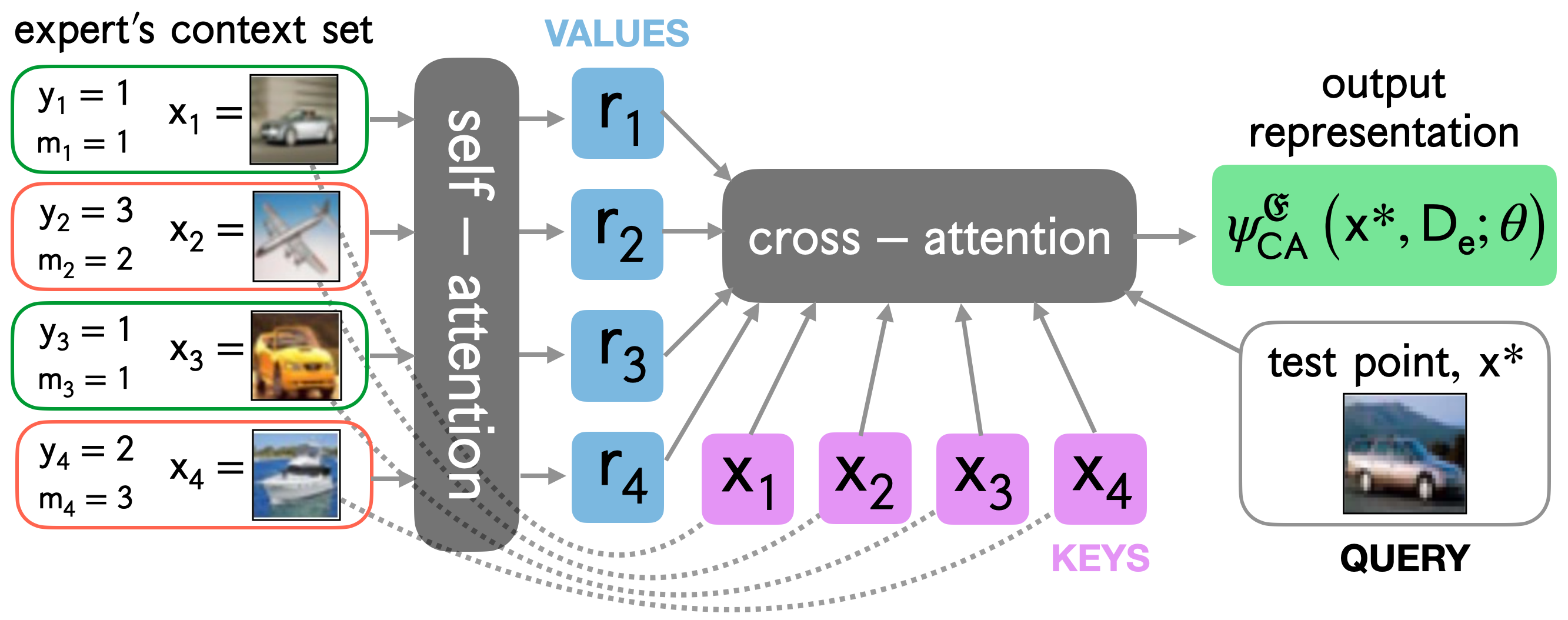
Figure 1: Attentive Encoder of Expert’s Context Set. The above diagram shows how an expert’s context set is summarized into a representation. The cross-attention mechanism allows points in the context set to be emphasized if they are similar to the current query point. In the example above, images of cars would be emphasized to determine if this expert performs well at classifying cars.

4 META-LEARNING TO DEFER

While we have given a complete recipe for L2D-Pop, the above implementation relies upon having an effective way to summarize the expert via the feature vector ${\bm{\psi}}^{\mathfrak{E}}$. However, specifying these features will greatly depend on the application and having domain knowledge. For cases without strong prior knowledge, we now describe a general meta-learning approach that allows the rejector to leverage whole (but likely small) data sets that are representative of the current expert’s decision making.

Context Set

Instead of using handcrafted features, we now assume that the model has access to a small but representative set of demonstrations for any given expert. Denote this context set for the $e$-th expert as:

$$\mathcal{D}_{e}=\left\{{\textnormal{d}}_{e,b}\right\}_{b=1}^{B}=\left\{({\mathbf{x}}_{e,b},{\textnormal{y}}_{e,b},{\textnormal{m}}_{e,b})\right\}_{b=1}^{B}$$

where $B$ is the size of the set. Ideally these demonstrations should have been collected recently. This set should also be as large as possible without burdening the expert’s time (what constitutes a ‘burden’ will depend on the effort it takes the expert to produce each prediction). For the radiology example, the context set could be obtained by having the doctor perform a few ‘warm-up’ diagnoses (on historical data) before commencing her real shift.

4.1 Meta-Optimization Approach

A straight-forward method for learning from the context set $\mathcal{D}_{e}$ is via meta-optimization. In its most basic implementation, this approach takes the form of fine-tuning. First train the L2D-Pop system to model the marginal expert via the surrogate ${\upphi}_{\text{SM-Pop-Avg}}$ from Section 3.3. Then at test time, when a new expert is available, perform gradient descent updates using $\mathcal{D}_{e}$. This will adapt the L2D-Pop system to move away from modeling the marginal expert and (hopefully) towards modeling the newly available one.

One can also employ model-agnostic meta-learning (MAML) (Finn et al., 2017) for L2D-Pop. MAML aims to make the model amenable to test-time fine-tuning by simulating fine-tuning during training. Ultimately, we found that using MAML made it hard to balance the performance of the classifier and rejector; see App. C for further details and the results. Traditional fine-tuning was more stable, and for this reason, we report its performance in the experiments as representative of the meta-optimization approach.

4.2 Model-Based Approach

We now describe a model-based approach to meta-learning for L2D-Pop. Instead of using optimization to adapt the model, the entire context set will be used as input to a (data) set encoder. This encoder then performs the adaptation via one forward pass.

Deep Sets Encoder

Given the context set $\mathcal{D}_{e}$ describing the expert’s decision making, we can encode it into a representation via a deep sets architecture (Zaheer et al., 2017). While there are several choices available, we use the mean aggregation mechanism employed by neural processes (Garnelo et al., 2018). Let ${\mathbf{r}}={\bm{\upgamma}}({\textnormal{d}};{\bm{\uptheta}})$ denote the output of a neural architecture (e.g. multi-layer perceptron or ConvNet), with parameters ${\bm{\uptheta}}$, applied to a point in the expert’s context set, d. Applying mean aggregation to the output of ${\bm{\upgamma}}$, the expert’s representation is:

$${\bm{\psi}}^{\mathfrak{E}}\left(\mathcal{D}_{e};{\bm{\uptheta}}\right)=\frac{1}{B}\sum_{b=1}^{B}{\mathbf{r}}_{e,b}=\frac{1}{B}\sum_{b=1}^{B}{\bm{\upgamma}}({\textnormal{d}}_{e,b};{\bm{\uptheta}}),$$

where ${\bm{\uptheta}}$ needs to be fit along with the other parameters of the L2D system. The deferral function is then composed with the output of the set encoder: $g_{\bot}\left({\bm{x}},{\bm{\psi}}^{\mathfrak{E}}\left(\mathcal{D}_{e};{\bm{\uptheta}}\right)\right)$.

Cross-Attention Mechanism

One drawback of the mean pooling mechanism is that all points are weighted equally. However, even if an expert is an overall poor decision maker, if they make good predictions on points similar to the current test point, then this could be reason enough to defer to them. Following the attentive neural process (Kim et al., 2019), we apply cross-attention between $\mathcal{D}_{e}$ and a test-point ${\mathbf{x}}$. Figure 1 shows a diagram of the computation, which also includes an optional self-attention mechanism to generate richer representations of $\mathcal{D}_{e}$. In the figure, the test point ${\mathbf{x}}^{*}$ is an image of a car, and thus cross-attention should up-weight the first and third points in the context set, as they also contain cars. We denote the output of the cross-attention mechanism as ${\bm{\psi}}_{\text{CA}}^{\mathfrak{E}}\left({\mathbf{x}},\mathcal{D}_{e};{\bm{\uptheta}}\right)$, and in turn, the deferral function is $g_{\bot}\left({\mathbf{x}},{\bm{\psi}}_{\text{CA}}^{\mathfrak{E}}\left({\mathbf{x}},\mathcal{D}_{e};{\bm{\uptheta}}\right)\right)$, where ${\mathbf{x}}$ is an input to both the deferral function and the expert representation learner.

Missing Demonstrations at Test Time

One may worry that, at test time, an expert can appear who does not have a corresponding context set. Such a situation is easy to handle with meta-optimization since the model can simply remain fixed to model the marginal expert (which is a good inductive bias). On the other hand, there is no guarantee for how the set encoder will behave if given the empty set as input. If this is a worry, one could train a second L2D system that models the marginal expert (from Section 3.3) and use it instead for expert’s with empty context sets. Yet, in Section D.2 we show that our neural process does not defer when the context set is missing: coverage is nearly 99%. This is an appropriate behavior since, if the model does not have any information about the available expert, then not deferring is a safe decision. One could also try to use the imputation method of Hemmer et al. (2023) to fill in the missing values.

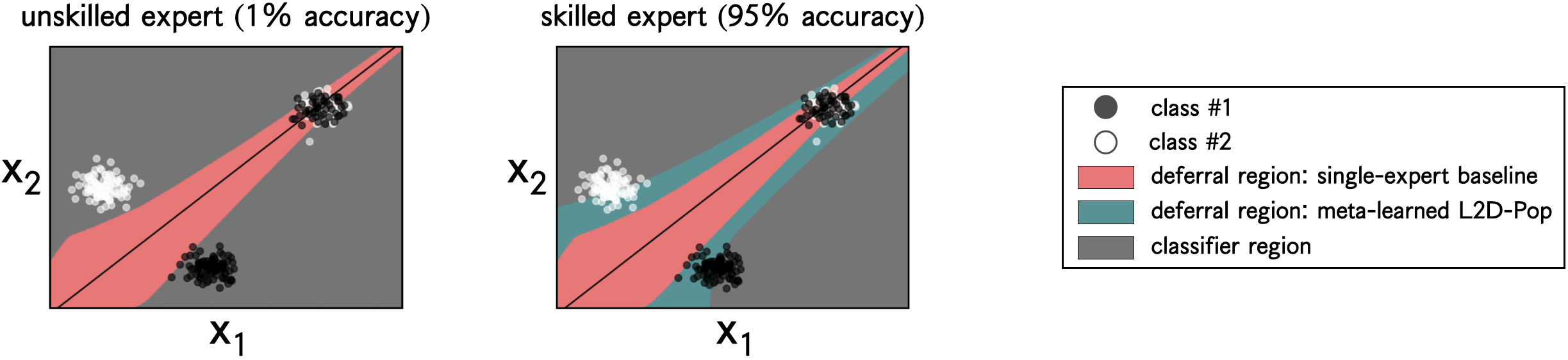
Figure 2: Synthetic 2D Data. We simulate three clusters, two having class purity and a third having a mixture of two classes. Furthermore, we simulate three experts and show the model’s decision regions for the worst ($1\%$) and best ($95\%$). The red region is where single-expert L2D defers; it is constant across experts. The green region is where L2D-Pop defers; it successfully adapts to the expert by never deferring the former case and deferring the whole of the difficult cluster in the latter case.

5 RELATED WORK

Classifiers with the ability to reject or abstain have long been studied (Chow, 1957), with Madras et al. (2018) developing the modern formulation that we consider. The two primary approaches to making the rejection decision have been confidence-based (Bartlett and Wegkamp, 2008; Yuan and Wegkamp, 2010; Jiang et al., 2018; Grandvalet et al., 2009; Ramaswamy et al., 2018; Ni et al., 2019) and model-based (Cortes et al., 2016b, a). The theoretical properties of the classifier-rejector approach have been well-studied for binary (Cortes et al., 2016b, a) and multi-class classification (Ni et al., 2019; Charoenphakdee et al., 2021; Mozannar and Sontag, 2020; Cao et al., 2022). There are also various L2D relatives that do not come with consistency guarantees (Raghu et al., 2019; Wilder et al., 2020; Pradier et al., 2021; Okati et al., 2021; Liu et al., 2022). Several limitations of the current L2D algorithms have also been studied, including mis-calibration (Verma and Nalisnick, 2022; Cao et al., 2023), under-fitting (Narasimhan et al., 2022), realizable consistency (Mozannar et al., 2023), sample complexity (Charusaie et al., 2022), and data scarcity (Hemmer et al., 2023). As for L2D systems that support multiple experts, existing formulations (Keswani et al., 2021; Hemmer et al., 2022; Verma et al., 2023; Mao et al., 2023, 2024) all consider a finite number of experts and assume they are seen during training. Our meta-learning approach most resembles the work of Hemmer et al. (2023), as they try to cope with missing expert demonstrations via model-based imputation. But they do not consider incorporating this model into a different or more general L2D framework, which is our primary contribution.

6 EXPERIMENTS

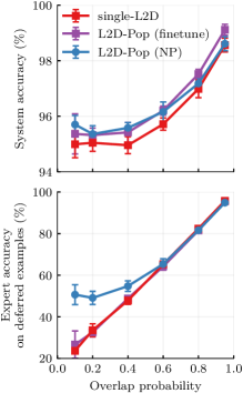
(a) Traffic Signs

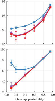
(b) CIFAR-10

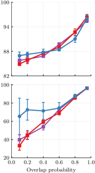
(c) HAM10000

Figure 3: Varying Population Diversity on Image Classification Tasks. L2D-Pop exploits experts’ context sets to make better deferment decisions given by the increase in expert accuracy on deferred examples (bottom). This leads to a boost in overall system accuracy (top). The gap widens as the overlap in experts’ abilities decreases.

We perform a range of experiments that isolate the effectiveness of L2D-Pop as the underlying population changes. Our implementation is available at https://github.com/dvtailor/meta-l2d. The primary baseline we considered is a single-expert L2D system (single-L2D) that models the population average, as described in Section 3.3. This is an informative baseline since single-L2D and L2D-Pop will converge in performance as the population becomes concentrated around the mean expert. We use the softmax-based surrogate loss for all results below. Results for one-vs-all surrogates are included in Section D.1.

6.1 Synthetic 2D Data

We first perform a simulation to demonstrate the failure of modeling just the population average, as single-L2D does. We simulate a binary classification task by drawing the features from one of three Gaussian distributions (${\bm{\mu}}=\{[10,10],[2,6],[6,2]\}$, $\Sigma=\text{diag}\{[0.2,0.2]\}$), with the Gaussian located at $[10,10]$ having a 50-50 mixture of classes and the other two clusters having $100\%$ class purity. We construct three experts who make predictions across the feature space with a uniform correctness probability of $\{0.01,0.80,0.95\}$. Here we consider just the model-based variant of L2D-Pop: the deferral function is parameterized by a neural process. We use a linear model for the classifier, and the context embedding network and rejector network are parameterized by $3$-layer and $2$-layer MLPs respectively. We sample $6000$ training examples, and context sets of size $B=60$ are sampled from the train set.

Figure 2 shows the model’s decision regions when the worst ($1\%)$ and best ($95\%$) experts are available. Single-L2D is not adaptive and has the same decision region in both cases. It fails by over-deferring in the former case, as the expert will do even worse than random chance on the third cluster. Conversely, it under-defers in the latter case, as the model has only a random chance of being correct on the third cluster. L2D-Pop successfully adapts to both settings, never deferring when the expert is poor and deferring the whole third cluster when the expert is good.

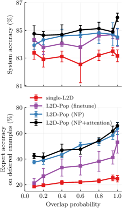
Figure 4: L2D-Pop implemented with an attentive neural process (black) boosts performance when experts’ abilities are specified by side-information (fine-grained labels) not provided in the context set.

6.2 Varying Population Diversity

Data Sets

We evaluate two variants of L2D-Pop, one implemented with meta-optimization (finetune) and the other with model-based meta-learning (NP). For data sets, we use CIFAR-10, Traffic Signs (Houben et al., 2013), and HAM10000 (Tschandl et al., 2018) for skin lesion diagnosis. Our meta-learning models are compared against a L2D system that models the marginal expert (single-L2D). For Traffic Signs, we downsample the train set to 10,000 instances. During training, context sets are sampled from the train set, each containing 50 instances for Traffic Signs and CIFAR-10, and 140 for HAM10000. During evaluation, context sets are sampled from a 20% split of the validation and test sets.

Models

We follow the approach of Mozannar and Sontag (2020), using a single base network. For L2D-Pop, the penultimate hidden activations of the base network are concatenated with the context embedding, and this is passed to a rejector network with a single output. The base network for CIFAR-10 is a WideResNet with 28 layers and the base network for HAM10000 is a ResNet-34. We warm-start these networks using model parameters from training the classifier only. The base network for Traffic Signs is a ResNet-20 (trained without warm-starting). All networks are trained without data augmentation. See Section B.1 for further details on the training configuration.

Expert Population

We construct synthetic experts by sampling without replacement classes for which the expert is an oracle. For non-oracle classes, the expert is correct with probability $p$ and otherwise predicts uniformly at random. $p$ is an overlap probability which we increase from $0.1$ to $0.95$, toggling from specialized to identical experts, thereby representing the diversity of the expert population. We sample $10$ experts at train-time. For evaluation, we remove 5 of these and sample 5 new experts (simulating never-before-seen experts). However, unlike during training where all ten experts are used, during evaluation only one expert is queried at a time (selected at random) for each new test point. The number of oracle classes per expert is one for CIFAR-10 and HAM10000, and five for Traffic Signs (due to it having many classes).

Results

Figure 3 shows the combined accuracy of the classifier and expert versus the overlap probability $p$ (top) and the expert’s accuracy on only deferred examples (bottom). When the expert population is at its most diverse (far left), L2D-Pop is clearly superior at deferring, as shown by the expert accuracy on deferred examples, leading to an improved system accuracy over the single-expert baseline. This improvement is more pronounced for the model-based (neural process) implementation. The gap narrows as the overlap across experts increases, as is expected. The neural process model also has faster adaptation as it does not need to run gradient updates at test-time; see Table 2 for a comparison of runtime.

6.3 Ablation Study of Attention

We study the effect of cross-attention in the neural process by taking CIFAR-100 and merging the 100 classes into 20 superclasses of equal size. Unless otherwise stated, we follow the same setup as in Section 6.2. We use context sets of size 100. See Section B.2 for the details of the model architectures. While the model predicts on the 20 superclasses, the 100 subclasses are used to construct experts with finer granularity. For each expert, we sample 4 superclasses uniformly at random without replacement. Then within these superclasses we pick 3 out of 5 subclasses at random. This gives a total of 12 subclasses for which the expert gives correct predictions. Outside of these subclasses, but within the superclasses, with overlap probability $p$ the expert is correct. Otherwise the expert predicts uniformly at random amongst the superclasses. This hierarchical formulation allows us to experimentally verify that the model with cross-attention can better select experts by identifying if they are oracles for any subclasses within the superclasses. Figure 4 reports the results. Cross-attention improves performance compared to the vanilla NP architecture, and especially compared to fine-tuning the marginal-expert model.

7 CONCLUSIONS

We proposed learning to defer to a population (L2D-Pop), a generalization of learning to defer that allows for never-before-seen experts at test time. This is achieved by training the model to generalize its deferral sub-component to all experts in a population. We described two meta-learning implementations that adapt to any expert using a context set of demonstrations. Our model is effective on data sets for traffic sign recognition and skin lesion diagnosis, especially as expert variability increases. For future work, we plan to investigate alternative methods for meta-learning, such as metric-based approaches. Moreover, the natural next step is to consider experts who change after training and therefore introduce distribution shift to the L2D problem.

Acknowledgements

This publication is part of the project Continual Learning under Human Guidance (VI.Veni.212.203), which is financed by the Dutch Research Council (NWO). Putra Manggala was supported by the Hybrid Intelligence Center, a $10$-year program funded by the Dutch Ministry of Education, Culture and Science through the Netherlands Organisation for Scientific Research. Part of this work was carried out on the Dutch national e-infrastructure with the support of the SURF Cooperative.

 

Learning to Defer to a Population: A Meta-Learning Approach
Supplementary Material

 

Appendix A THEORETICAL RESULTS

In this section, we provide proofs of the main results in the paper. The proofs follow from the results of Verma et al. (2023). We follow the notation from the paper. For simplicity, we assume all measure theoretic subtleties hold true.

A.1 Bayes Solution for L2D to a population

The Bayes solution of L2D to a population follows directly from Proposition A.2 and Corollary A.3 of Verma et al. (2023). In particular, for an expert $\mathfrak{C}\sim\mathbb{P}\left(\mathfrak{C}\right)$ and ${\mathbf{x}}\sim\mathbb{P}({\mathbf{x}})$, their proposition can be extended to give the rejection rule $r^{*}\left({\mathbf{x}},\mathfrak{C}\right)$ as below:

$$\begin{split}r^{*}\left({\mathbf{x}},\mathfrak{C}\right)=\begin{cases}1\textrm{ if }\mathbb{E}_{{\textnormal{y}}|{\mathbf{x}}}\left[\ell_{\text{clf}}\left(\hat{{\textnormal{y}}},{\textnormal{y}}\right)\right]\geq\mathbb{E}_{{\textnormal{y}}|{\mathbf{x}}}\mathbb{E}_{{\textnormal{m}}_{\mathfrak{C}}|{\mathbf{x}},{\textnormal{y}},\mathfrak{C}}\left[\ell_{\text{exp}}\left({\textnormal{m}}_{\mathfrak{C}},{\textnormal{y}}\right)\right]\forall\hat{y}\in\mathcal{Y},\\ 0\textrm{ otherwise },\end{cases}\end{split}$$ (9)

where $\hat{y}$ is the prediction of the classifier, $\ell_{\text{clf}}$ and $\ell_{\text{exp}}$ are respectively the loss functions for the classifier and the expert. In this paper, we consider the canonical $0-1$ loss, $\mathbb{I}\left[\hat{{\textnormal{y}}}\neq{\textnormal{y}}\right]$ (equivalently, $\mathbb{I}\left[{\textnormal{m}}_{\mathfrak{C}}\neq{\textnormal{y}}\right]$), in which case the Bayes rejection rule follows immediately.

A.2 Consistency of ${\upphi}_{\text{SM-Pop}}$ (Equation 7)

Define $-\log\left(\frac{\exp\{g_{y}\left({\bm{x}}\right)\}}{\mathcal{Z}\left({\bm{x}},\mathbf{\psi}_{e}^{\mathfrak{C}}\right)}\right)=\zeta_{y}\left({\bm{x}}\right)$ and $-\log\left(\frac{\exp\{g_{\bot}\left({\bm{x}},\mathbf{\psi}_{e}^{\mathfrak{C}}\right)\}}{\mathcal{Z}\left({\bm{x}},\mathbf{\psi}_{e}^{\mathfrak{C}}\right)}\right)=\zeta_{\bot,e}\left({\bm{x}}\right)$. We consider the point-wise risk for ${\upphi}_{\text{SM-Pop}}$ written in terms of these terms as,

$$\begin{split}\mathcal{C}\left({\upphi}_{\text{SM-Pop}}\right)&=\sum_{e=1}^{E}\left[\mathbb{E}_{{\textnormal{y}}|{\bm{x}}}\left[\zeta_{y}\left({\bm{x}}\right)\right]+\mathbb{E}_{{\textnormal{y}}|{\bm{x}}}\mathbb{E}_{{\textnormal{m}}|{\bm{x}},y,e}\left[\mathbb{I}\left[m_{e}=y\right]\cdot\zeta_{\bot,e}\left({\bm{x}}\right)\right]\right]\\ &=\sum_{e=1}^{E}\left[\sum_{y\in\mathcal{Y}}\mathbb{P}\left(y|{\bm{x}}\right)\zeta_{y}\left({\bm{x}}\right)+\sum_{y\in\mathcal{Y}}\mathbb{P}\left(y|{\bm{x}}\right)\sum_{m_{e}\in\mathcal{Y}}\mathbb{P}\left({\textnormal{m}}=m_{e}|{\bm{x}},y,e\right)\mathbb{I}\left[m_{e}=y\right]\cdot\zeta_{\bot,e}\left({\bm{x}}\right)\right]\\ &=\sum_{e=1}^{E}\left[\sum_{y\in\mathcal{Y}}\mathbb{P}\left(y|{\bm{x}}\right)\zeta_{y}\left({\bm{x}}\right)+\sum_{y\in\mathcal{Y}}\mathbb{P}\left({\textnormal{y}}=y|{\bm{x}}\right)\mathbb{P}\left({\textnormal{m}}=y|{\bm{x}},y,e\right)\cdot\zeta_{\bot,e}\left({\bm{x}}\right)\right]\\ &=\sum_{e=1}^{E}\left[\sum_{y\in\mathcal{Y}}\mathbb{P}\left(y|{\bm{x}}\right)\zeta_{y}\left({\bm{x}}\right)+\sum_{y\in\mathcal{Y}}\mathbb{P}\left({\textnormal{m}}=y,{\textnormal{y}}=y|{\bm{x}},e\right)\cdot\zeta_{\bot,e}\left({\bm{x}}\right)\right]\\ &=\sum_{e=1}^{E}\left[\sum_{y\in\mathcal{Y}}\mathbb{P}\left(y|{\bm{x}}\right)\zeta_{y}\left({\bm{x}}\right)+\mathbb{P}\left({\textnormal{m}}={\textnormal{y}}|{\bm{x}},e\right)\cdot\zeta_{\bot,e}\left({\bm{x}}\right)\right].\end{split}$$

Considering that the above expression is a sum of $E$ convex terms, we can obtain the minimizer of the point-wise risk easily by differentiating the above expression w.r.t. $g_{y}\left({\bm{x}}\right)$ and $g_{\bot}\left({\bm{x}},\psi_{e}^{\mathfrak{C}}\right)$. The crucial observation we make here is that $\bm{\psi}_{e}^{\mathfrak{C}}$ is a constant (the context associated with the expert if fixed). The said minimizers then satisfy the following conditions (for each $e$):

$$\begin{split}&\frac{\partial\mathcal{C}\left[{\upphi}_{\text{SM-Pop}}\right]}{\partial g_{y}\left({\bm{x}}\right)}=0\implies\frac{\exp g_{y}\left({\bm{x}}\right)}{\mathcal{Z}\left({\bm{x}},\bm{\psi}_{e}^{\mathfrak{C}}\right)}=\frac{\mathbb{P}\left({\textnormal{y}}=y|{\mathbf{x}}={\bm{x}}\right)}{1-\mathbb{P}\left({\textnormal{m}}={\textnormal{y}}|{\bm{x}},e\right)},\textrm{ and }\\ &\frac{\partial\mathcal{C}\left[{\upphi}_{\text{SM-Pop}}\right]}{\partial g_{\bot}\left({\bm{x}},\bm{\psi}_{e}^{\mathfrak{C}}\right)}=0\implies\frac{\exp g_{\bot}\left({\bm{x}},\bm{\psi}_{e}^{\mathfrak{C}}\right)}{\mathcal{Z}\left({\bm{x}},\bm{\psi}_{e}^{\mathfrak{C}}\right)}=\frac{\mathbb{P}\left({\textnormal{m}}={\textnormal{y}}|{\bm{x}},e\right)}{1-\mathbb{P}\left({\textnormal{m}}={\textnormal{y}}|{\bm{x}},e\right)}.\end{split}$$

Given how the rejection and prediction is set up in ${\upphi}_{\text{SM-Pop}}$ and these conditions, it follows that the minimizer of the point-wise risk adheres to the Bayes solution. Considering the hypothesis class of all functions, consistency follows.

A.3 One-vs-All (OvA) surrogate for L2D to a population

In the main text, we considered softmax version of the surrogate loss. We can also extend the OvA version of the surrogate loss for L2D proposed by Verma and Nalisnick (2022) for L2D to a population, as given below:

$$\begin{split}&{\upphi}_{\text{OvA-Pop}}\left(g_{1},\ldots,g_{K};{\bm{x}},y,\{m_{e},\bm{\psi}_{e}^{\mathfrak{C}}\}_{e=1}^{E}\right)=\\ &\sum_{e=1}^{E}\phi\left(g_{y}\left({\bm{x}}\right)\right)+\phi\left(-g_{\bot}\left({\bm{x}},\bm{\psi}_{e}^{\mathfrak{C}}\right)\right)+\sum_{y^{\prime}\in\mathcal{Y}/\{y\}}\phi\left(-g_{y}\left({\bm{x}}\right)\right)+\mathbb{I}\left[m_{e}=y\right]\left[\phi\left(g_{\bot}\left({\bm{x}},\bm{\psi}_{e}^{\mathfrak{C}}\right)\right)-\phi\left(-g_{\bot}\left({\bm{x}},\bm{\psi}_{e}^{\mathfrak{C}}\right)\right)\right],\end{split}$$

where $\phi$ is some classification-calibrated (Bartlett et al., 2006) binary surrogate loss function, e.g. the logistic loss. It is easier to establish the consistency of ${\upphi}_{\text{OvA-Pop}}$ following Theorem 1 in Verma and Nalisnick (2022).

Appendix B EXPERIMENTAL DETAILS FOR IMAGE CLASSIFICATION TASKS

B.1 Varying Population Diversity

The base network is trained using SGD with Nesterov momentum (default momentum parameter of 0.9). The other model components (final layer of the classifier, rejector and context embedding network) are trained using Adam. We use a cosine learning rate decay scheme, annealing the learning rate to $\frac{LR_{\text{cnn}}}{1000}$ and $\frac{LR}{1000}$ for the base network and remaining model components respectively, until $T_{e}\!-\!50$ epochs. For the last $50$ epochs, the base learning rate is held constant at $\frac{LR_{\text{cnn}}}{1000}$ and $\frac{LR}{1000}$ for the respective model components. We train without data augmentation nor do we use state-of-the-art network architectures as it is not our intention to obtain best classifier performance.

A checkpoint of the model is saved only if an improvement in the model performance is observed after every epoch. Nevertheless, training always runs for the full number of epochs stated but only the checkpointed model is evaluated on. We use the validation loss to score models except for HAM10000 where we use the system accuracy. We use a batch size of 8 and 1 for the validation set and test set respectively – for each minibatch, the expert is sampled anew and a new context set is drawn. We also perform warmstarting for some of the experiments. The warmstart parameters are obtained by training the classifier only. This is done in the same way as the L2D system except we train for a fixed number of epochs (100 for HAM10000 and 200 for the others) without intermediate model checkpointing and use a cosine learning rate decay scheme where the learning rate is annealed to 0. A base learning rate of $10^{-2}$ is used for HAM10000 and the others use $10^{-1}$. In the case of HAM10000, the warmstart parameters are obtained by fine-tuning from pretrained weights on ImageNet. For fine-tuning the marginal single-expert L2D, we perform a grid search using the validation loss over the number of steps $[1,2,5,10,20]$ and step size $[10^{-3},10^{-2}]$ for HAM10000 and $[10^{-2},10^{-1}]$ for the others. The fine-tuning is performed with vanilla gradient-descent where the base network parameters are frozen (i.e. only update the classifier and rejector final layer).

We now proceed to describe the context embedding network architecture. First the base network is used to extract a feature vector for context inputs (corresponding to the penultimate layer activations). We note that during training, we disable gradients backpropagating to the base network from the context embedding. Next context labels and expert predictions are embedded using a linear layer with dimensionality $128$. The above are then concatenated and passed to a MLP with width $128$ that outputs an embedding of $128$ dimensions. This is repeated for all context points, the resulting embeddings for each context point are mean-pooled giving an aggregate embedding for the whole context set which acts as a proxy for the expert representation. The rejector network is also given by a MLP with width $128$ that takes the extracted features for the test point (resulting from the base network) and the context embedding as input and outputs a single unit for the rejector logit.

The data sets are preprocessed as follows: for CIFAR-10, $10\%$ of the train set is used for the validation set. For Traffic Signs, the provided train set is downsampled to $10000$ examples and the provided test set is split $50{-}50$ into valid/test sets that we use. For HAM10000, the data set is prepared in the same way as (Verma and Nalisnick, 2022) (60% train, 20% valid and 20% test splits). The experiments were run on an internal cluster of GPUs of the following type: Tesla V100 SXM2 16 GB.

Data Set	Base Network	Warm-Starting	Batch Size	$T_{e}$	$K$	$LR_{\text{cnn}}$	$LR$	$\delta$	$B$	$\ell_{\text{emb}}$	$\ell_{\text{rej}}$
Traffic Signs	ResNet-20	✕	$64$	$150$	$43$	$10^{-2}$	$10^{-3}$	$10^{-3}$	$50$	$5$	$3$
CIFAR-10	WideResNet-28-2	✓	$128$	$100$	$10$	$10^{-2}$	$10^{-3}$	$5\!\times\!10^{-4}$	$50$	$6$	$4$
HAM10000	ResNet-34	✓	$128$	$100$	$7$	$10^{-2}$	$10^{-3}$	$5\!\times\!10^{-4}$	$140$	$6$	$4$
CIFAR-20	WideResNet-28-4	✓	$128$	$100$	$20$	$10^{-2}$	$10^{-3}$	$5\!\times\!10^{-4}$	$100$	$6$	$4$

Table 1: Hyperparameters for image classification experiments: number of epochs $T_{e}$, number of classes $K$, initial learning rate of the CNN base network $LR_{\text{cnn}}$, initial learning rate of remaining model components $LR$, weight decay on CNN base network parameters $\delta$, context set size $B$, number of MLP layers for embedding network $\ell_{\text{emb}}$, number of MLP layers for rejector network $\ell_{\text{rej}}$.

B.2 Ablation Study of Attention

Unless otherwise stated, the experimental setup follows Section B.1 with specific hyperparameters given in Table 1. We use data augmentation involving random horizontal flipping and random cropping. This is also used to obtain the warmstart parameters. A separate base network is trained for the classifier and rejector. The base network for the rejector is used to extract features for context inputs (and we also allow gradients to backpropogate in contrast to Section B.1). We evaluate an additional meta-learning architecture where the context embedding network contains attention mechanisms (rejector network is unchanged). This follows the design of the Attentive Neural Process (deterministic path) (Kim et al., 2019) with a self-attention layer first applied over individual context embeddings followed by a cross-attention layer. We use multi-head attention (Vaswani et al., 2017) with 8 heads throughout. The number of parameters, training time and prediction time of this setting is reported in Table 2. This highlights a trade-off between training runtimes and speed of test-time adaptation in the fine-tuning and neural process approaches to L2D-Pop.

Method	# Parameters	Training (s)	Prediction (s)
single-L2D	11698357	40.48	9.83
L2D-Pop (finetune)	11698357	40.48	248.38
L2D-Pop (NP)	11931317	148.90	14.57
L2D-Pop (NP w/ attention)	12063413	163.33	15.11

Table 2: Number of parameters, training time and prediction time of L2D-Pop and the single-expert L2D baseline on the CIFAR-20 data set. Training run time is measured for a single epoch (352 batches of size 128). Prediction run time is measured over a full pass over the validation set (5000 examples) with batch size 8. For L2D-Pop (finetune), this is only measured for a step size of $10^{-1}$ and 5 steps (time for grid search not included). A NVIDIA GeForce RTX 3090 was used to obtain these runtimes.

Appendix C META-OPTIMIZATION USING MAML

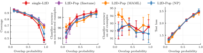
(a) Traffic Signs

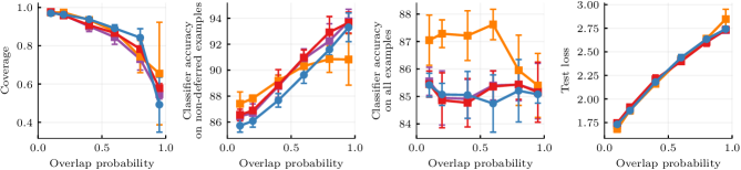
(b) CIFAR-10

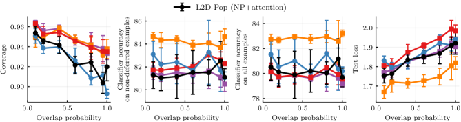
(c) CIFAR-20

Figure 11: Additional metrics for MAML experiment.

We evaluate an additional meta-optimization approach to L2D-Pop using MAML (see Algorithm 1). Evaluating MAML in our existing setup led to poor performance which we determined was the result of using batch normalization in the base networks. In the original MAML implementation by Finn et al. (2017), minibatch statistics are used during both train and test time (that is the batch normalization layers do not track running statistics) and it is assumed evaluation data is also minibatched (see (Antoniou et al., 2018) for further details). In contrast, our setup queries each test example one at a time. To ensure a fair comparison between all approaches to L2D-Pop and the single-expert baseline, we replaced batch normalization with filter response normalization (Singh and Krishnan, 2020) that does not depend on minibatch statistics. Otherwise the experimental setup is the same as that in App. B. This leads to lower classifier accuracy as reported in Fig. 11. There are alternatives developed specifically for meta-learning such as meta-batch normalization (Bronskill et al., 2020) but we could not get it to work for our MAML implementation applied to Pop-L2D. We leave a more thorough investigation of normalization layers in the case of meta-optimization for Pop-L2D to future work.

MAML for Pop-L2D has two additional hyperparameters, step size and number of steps, for train-time fine-tuning. We specify the following grid, step size $[10^{-2},10^{-1}]$ and the number of steps $[1,2,5]$. Due to computational restrictions, we only perform a grid search on these hyperparameters for a single setting of overlap probability $p=0.1$ for each data set (using validation loss as scoring criterion). The best combination is then used across all $p$. The only exception is on Traffic Signs for which we observed unstable training for $p\geq 0.4$ and so the hyperparameters were retuned on $p=0.4$. In summary, the tuned train-time hyperparameters are as follows: for CIFAR-10 and CIFAR-20, we found a step size of $10^{-1}$ and 2 steps was the best; in the case of Traffic Signs, we used a step size of $10^{-1}$ and 5 steps for $p\in(0.1,0.2)$ and then a reduced step size of $10^{-2}$ for $p\geq 0.4$. For fine-tuning at evaluation, we used the same step size as during training but allowed the number of steps to be re-tuned (again on the validation loss) on entries in $[1,2,5,10,20]$ greater than or equal to the train-time step count. We typically observed the selected number of steps at evaluation to be slightly larger than that used during training – this is similar to what was reported in (Finn et al., 2017). Similar to App. B, we use vanilla gradient-descent and the base network parameters are frozen during fine-tuning, both train and test-time. However, in contrast to test-time fine-tuning, we also freeze the classifier parameters (last layer) during train-time fine-tuning (i.e. only fine-tune the rejector). For the meta-optimization step, we use the implementation of first-order MAML (Finn et al., 2017).

L2D-Pop with MAML along with the other approaches to L2D-Pop and the single-expert baseline are shown in Fig. 7 (additional metrics are shown in Fig. 11). We observe that the MAML implementation consistently improves over test-time only fine-tuning as well as the single-expert baseline in terms of expert accuracy (bottom row). However, the neural process implementation of L2D-Pop remains competitive especially at the lower expert variability setting. Whilst we observe higher system accuracy for L2D-Pop with MAML, Fig. 11 verifies that this gain is largely due to the higher classifier accuracy.

Algorithm 1 L2D-Pop with MAML

0:  Step size $\alpha,\beta$, number of inner-optimization steps $S$, $E$ experts with context sets $\{\mathcal{D}_{e}\}_{e=1}^{E}$

1:  Initialize parameters of classifier $\theta^{\textrm{c}}$ and rejector $\theta^{\textrm{r}}$

2:  while not converged do

3:     for expert $e=1$ to $E$ do

4:        Initialize $\theta_{e}^{\textrm{r}}=\theta^{\textrm{r}}$

5:        for step = $1$ to $S$ do

6:           // Compute adapted rejector parameters by gradient descent on expert context set

7:           $\theta_{e}^{\textrm{r}}\leftarrow\theta_{e}^{\textrm{r}}-\alpha\nabla_{\theta_{e}}\sum_{b=1}^{B}{\upphi}_{\text{SM}}({\bm{g}}^{\theta^{\textrm{c}}},g_{\bot}^{\theta_{e}^{\textrm{r}}};{\textnormal{d}}_{e,b})$

8:        end for

9:     end for

10:     // Meta-update using adapted rejector parameters for each expert

11:     Sample $({\bm{x}},y,\{m_{e}\}_{e=1}^{E})$ from $\mathcal{D}$

12:     Update $\theta\leftarrow\theta-\beta\nabla_{\theta}{\upphi}_{\text{SM-Pop}}({\bm{g}},g_{\bot};{\bm{x}},y,\{m_{e},\theta_{e}^{\textrm{r}}\}_{e=1}^{E})$

13:  end while

Appendix D ADDITIONAL RESULTS

In Fig. 8, we provide additional metrics for the experiments shown in Figs. 3 and 4. In Fig. 9, we show the system accuracy as a function of the budget for three settings of the overlap probability $p\in\{0.1,0.4,0.8\}$ corresponding to high, medium and low expert population diversity. The budget is the upper limit on the proportion of examples that can be deferred to the expert. We refer the reader to App. E in (Verma and Nalisnick, 2022) for further details as well as details on the implementation. We observe L2D-Pop by single-expert fine-tuning is competitive against single-expert L2D for a range of budgets considered as well as different diversities of the expert population (not shown in the case of CIFAR-20 due to computational restrictions). This is also the case for L2D-Pop with neural process except on Traffic Signs and HAM10000 where it is shown to hold for the highest expert population diversity ($p=0.1$) however it is not observed at the lower expert population diversities which show more sensitivity to the budget.

D.1 One-vs-All (OvA) surrogate

In Figs. 5 and 10 we perform an ablation where we instead use the OvA surrogate loss for L2D-Pop and the single-expert baseline. All other experimental details are the same as stated in App. B except that a separate base network is trained for the classifier and rejector for all data sets (previously this was only done for CIFAR-20). Similar to the results with the softmax surrogate, we observe an increase in expert accuracy for both fine-tuning and the neural process implementation of L2D-Pop. Except for one setting of overlap probability $p=0.2$ in CIFAR-10, this leads to a boost in system accuracy.

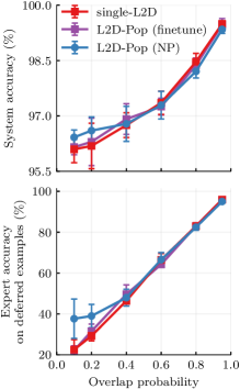
(a) Traffic Signs

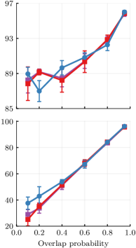
(b) CIFAR-10

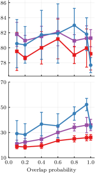
(c) CIFAR-20

Figure 5: Varying Population Diversity on Image Classification Tasks with OvA surrogate loss.

D.2 Missing context set at test-time

We investigate the behaviour of the neural process implementation of L2D-Pop when the context set is missing at test time. This is done on CIFAR-10 for the highest expert diversity setting: overlap probability of 0.95. Fig. 6 (left) reports the classifier coverage (y-axis) against the probability of observing the context set at test-time. Thus, at the far left, context sets are never observed, and at the far right, they are always observed. Our model simply does not defer when the context set is missing: coverage is nearly $99\%$ when the probability is 0. This is an appropriate behavior since, if the model does not have any information about the available expert, then not deferring is a safe decision. An example of inappropriate behavior would be making random deferral decisions—which, again, our model is not doing.

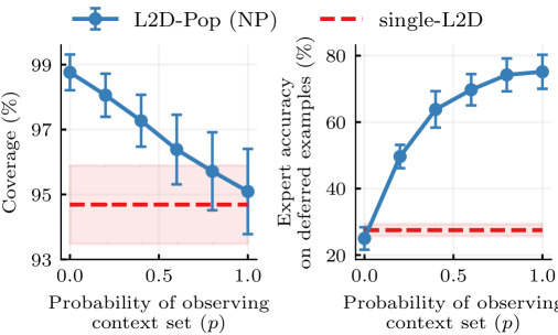
Figure 6: Investigation of the behaviour of L2D-Pop (NP) as the rate at which the context sets are excluded is varied at test-time, from always dropped ($p=0$) to always included ($p=1$). ‘Dropping’ means that we input only a zero vector. We emphasize that during training of L2D-Pop, context sets are always included ($p=1$). The results are shown on CIFAR-10 for the highest expert diversity setting. Single-expert L2D baseline is shown for comparison. We see that L2D-Pop simply uses the classifier more and more as context sets are increasingly missing (at test time).

(a) Traffic Signs

(b) CIFAR-10

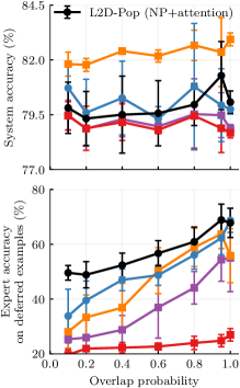
(c) CIFAR-20

Figure 7: Varying Population Diversity on Image Classification Tasks along with MAML approach to L2D-Pop.

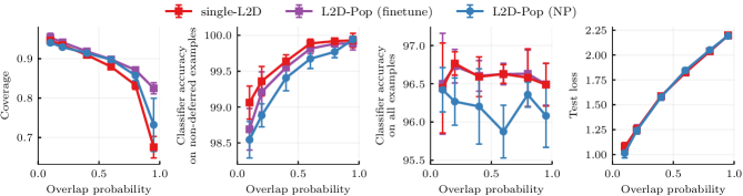
(a) Traffic Signs

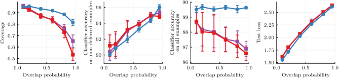
(b) CIFAR-10

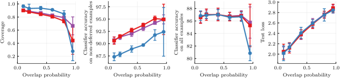
(c) HAM10000

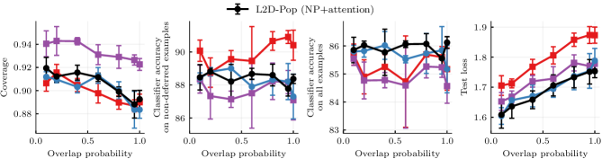
(d) CIFAR-20

Figure 8: Additional metrics for varying population diversity on image classification tasks.

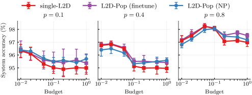
(a) Traffic Signs

(b) CIFAR-10

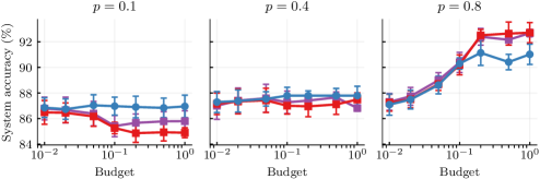
(c) HAM10000

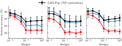
(d) CIFAR-20

Figure 9: System accuracy as a function of the budget for three settings of the overlap probability $p\in\{0.1,0.4,0.8\}$ corresponding to high, medium and low expert population diversity. This is shown for the data sets and baselines considered in varying population diversity on image classification tasks.

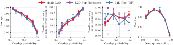
(a) Traffic Signs

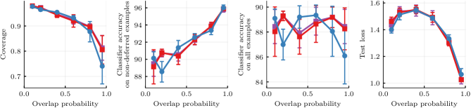
(b) CIFAR-10

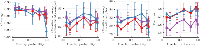
(c) CIFAR-20

Figure 10: Additional metrics for OvA experiment.

References

- Akata et al. (2020) Zeynep Akata, Dan Balliet, Maarten De Rijke, Frank Dignum, Virginia Dignum, Guszti Eiben, Antske Fokkens, Davide Grossi, Koen Hindriks, Holger Hoos, et al. A Research Agenda for Hybrid Intelligence: Augmenting Human Intellect With Collaborative, Adaptive, Responsible, and Explainable Artificial Intelligence. Computer, 2020.
- Andrychowicz et al. (2016) Marcin Andrychowicz, Misha Denil, Sergio Gomez, Matthew W. Hoffman, David Pfau, Tom Schaul, Brendan Shillingford, and Nando De Freitas. Learning to Learn by Gradient Descent by Gradient Descent. Advances in Neural Information Processing Systems, 2016.
- Antoniou et al. (2018) Antreas Antoniou, Harrison Edwards, and Amos Storkey. How to train your MAML. In Proceedings of the International Conference on Learning Representations, 2018.
- Bartlett and Wegkamp (2008) Peter L. Bartlett and Marten H. Wegkamp. Classification with a Reject Option Using a Hinge Loss. Journal of Machine Learning Research, 2008.
- Bartlett et al. (2006) Peter L. Bartlett, Michael I. Jordan, and Jon D. McAuliffe. Convexity, Classification, and Risk Bounds. Journal of the American Statistical Association, 2006.
- Bronskill et al. (2020) John Bronskill, Jonathan Gordon, James Requeima, Sebastian Nowozin, and Richard Turner. TaskNorm: Rethinking Batch Normalization for Meta-Learning. In Proceedings of the 37th International Conference on Machine Learning, 2020.
- Cao et al. (2022) Yuzhou Cao, Tianchi Cai, Lei Feng, Lihong Gu, Jinjie Gu, Bo An, Gang Niu, and Masashi Sugiyama. Generalizing Consistent Multi-Class Classification with Rejection to be Compatible with Arbitrary Losses. In Advances in Neural Information Processing Systems, 2022.
- Cao et al. (2023) Yuzhou Cao, Hussein Mozannar, Lei Feng, Hongxin Wei, and Bo An. In Defense of Softmax Parametrization for Calibrated and Consistent Learning to Defer. In Advances in Neural Information Processing Systems, 2023.
- Charoenphakdee et al. (2021) Nontawat Charoenphakdee, Zhenghang Cui, Yivan Zhang, and Masashi Sugiyama. Classification with Rejection Based on Cost-sensitive Classification. In Proceedings of the 38th International Conference on Machine Learning, 2021.
- Charusaie et al. (2022) Mohammad-Amin Charusaie, Hussein Mozannar, David Sontag, and Samira Samadi. Sample Efficient Learning of Predictors that Complement Humans. In Proceedings of the 39th International Conference on Machine Learning, 2022.
- Chow (1957) C. K. Chow. An Optimum Character Recognition System Using Decision Functions. IRE Transactions on Electronic Computers, 1957.
- Cortes et al. (2016a) Corinna Cortes, Giulia DeSalvo, and Mehryar Mohri. Boosting with Abstention. In Advances in Neural Information Processing Systems, 2016a.
- Cortes et al. (2016b) Corinna Cortes, Giulia DeSalvo, and Mehryar Mohri. Learning with Rejection. In Proceedings of the 27th International Conference on Algorithmic Learning Theory, 2016b.
- Dellermann et al. (2019) Dominik Dellermann, Philipp Ebel, Matthias Söllner, and Jan Marco Leimeister. Hybrid Intelligence. Business & Information Systems Engineering, 2019.
- Finn et al. (2017) Chelsea Finn, Pieter Abbeel, and Sergey Levine. Model-Agnostic Meta-Learning for Fast Adaptation of Deep Networks. In Proceedings of the 34th International Conference on Machine Learning, 2017.
- Foong et al. (2020) Andrew Y. K. Foong, Wessel P. Bruinsma, Jonathan Gordon, Yann Dubois, James Requeima, and Richard E. Turner. Meta-Learning Stationary Stochastic Process Prediction with Convolutional Neural Processes. In Advances in Neural Information Processing Systems, 2020.
- Garnelo et al. (2018) Marta Garnelo, Dan Rosenbaum, Christopher Maddison, Tiago Ramalho, David Saxton, Murray Shanahan, Yee Whye Teh, Danilo Rezende, and S. M. Ali Eslami. Conditional Neural Processes. In Proceedings of the 35th International Conference on Machine Learning, 2018.
- Gordon et al. (2020) Jonathan Gordon, Wessel P. Bruinsma, Andrew Y. K. Foong, James Requeima, Yann Dubois, and Richard E. Turner. Convolutional Conditional Neural Processes. In Proceedings of the International Conference on Learning Representations, 2020.
- Grandvalet et al. (2009) Yves Grandvalet, Alain Rakotomamonjy, Joseph Keshet, and Stéphane Canu. Support Vector Machines with a Reject Option. In Advances in Neural Information Processing Systems, 2009.
- Hemmer et al. (2022) Patrick Hemmer, Sebastian Schellhammer, Michael Vössing, Johannes Jakubik, and Gerhard Satzger. Forming Effective Human-AI Teams: Building Machine Learning Models that Complement the Capabilities of Multiple Experts. In International Joint Conference on Artificial Intelligence, 2022.
- Hemmer et al. (2023) Patrick Hemmer, Lukas Thede, Michael Vössing, Johannes Jakubik, and Niklas Kühl. Learning to Defer with Limited Expert Predictions. In Proceedings of the 37th AAAI Conference on Artificial Intelligence, 2023.
- Hospedales et al. (2021) Timothy Hospedales, Antreas Antoniou, Paul Micaelli, and Amos Storkey. Meta-Learning in Neural Networks: A Survey. IEEE Transactions on Pattern Analysis and Machine Intelligence, 2021.
- Houben et al. (2013) Sebastian Houben, Johannes Stallkamp, Jan Salmen, Marc Schlipsing, and Christian Igel. Detection of Traffic Signs in Real-World Images: The German Traffic Sign Detection Benchmark. In International Joint Conference on Neural Networks, 2013.
- Jiang et al. (2018) Heinrich Jiang, Been Kim, Melody Y. Guan, and Maya Gupta. To Trust or Not to Trust a Classifier. In Advances in Neural Information Processing Systems, 2018.
- Kamar (2016) Ece Kamar. Directions in Hybrid Intelligence: Complementing AI Systems with Human Intelligence. In International Joint Conference on Artificial Intelligence, 2016.
- Kawano et al. (2021) Makoto Kawano, Wataru Kumagai, Akiyoshi Sannai, Yusuke Iwasawa, and Yutaka Matsuo. Group Equivariant Conditional Neural Processes. In Proceedings of the International Conference on Learning Representations, 2021.
- Keswani et al. (2021) Vijay Keswani, Matthew Lease, and Krishnaram Kenthapadi. Towards Unbiased and Accurate Deferral to Multiple Experts. In Proceedings of the AAAI/ACM Conference on AI, Ethics, and Society, 2021.
- Kim et al. (2019) Hyunjik Kim, Andriy Mnih, Jonathan Schwarz, Marta Garnelo, Ali Eslami, Dan Rosenbaum, Oriol Vinyals, and Yee Whye Teh. Attentive Neural Processes. In Proceedings of the International Conference on Learning Representations, 2019.
- Leitão et al. (2022) Diogo Leitão, Pedro Saleiro, Mário A. T. Figueiredo, and Pedro Bizarro. Human-AI Collaboration in Decision-Making: Beyond Learning to Defer. ICML Workshop on Human-Machine Collaboration and Teaming, 2022.
- Liu et al. (2022) Jessie Liu, Blanca Gallego, and Sebastiano Barbieri. Incorporating Uncertainty in Learning to Defer Algorithms for Safe Computer-Aided Diagnosis. Scientific reports, 2022.
- Madras et al. (2018) David Madras, Toniann Pitassi, and Richard Zemel. Predict Responsibly: Improving Fairness and Accuracy by Learning to Defer. In Advances in Neural Information Processing Systems, 2018.
- Mao et al. (2023) Anqi Mao, Christopher Mohri, Mehryar Mohri, and Yutao Zhong. Two-Stage Learning to Defer with Multiple Experts. In Advances in Neural Information Processing Systems, 2023.
- Mao et al. (2024) Anqi Mao, Mehryar Mohri, and Yutao Zhong. Principled Approaches for Learning to Defer with Multiple Experts. International Symposium on Artificial Intelligence and Mathematics, 2024.
- Mozannar and Sontag (2020) Hussein Mozannar and David A. Sontag. Consistent Estimators for Learning to Defer to an Expert. In In Proceedings of the 37th International Conference on Machine Learning, 2020.
- Mozannar et al. (2023) Hussein Mozannar, Hunter Lang, Dennis Wei, Prasanna Sattigeri, Subhro Das, and David Sontag. Who Should Predict? Exact Algorithms For Learning to Defer to Humans. In Proceedings of the 26th International Conference on Artificial Intelligence and Statistics, 2023.
- Narasimhan et al. (2022) Harikrishna Narasimhan, Wittawat Jitkrittum, Aditya Krishna Menon, Ankit Singh Rawat, and Sanjiv Kumar. Post-hoc Estimators for Learning to Defer to an Expert. In Advances in Neural Information Processing Systems, 2022.
- Ni et al. (2019) Chenri Ni, Nontawat Charoenphakdee, Junya Honda, and Masashi Sugiyama. On the Calibration of Multiclass Classification with Rejection. In Advances in Neural Information Processing Systems, 2019.
- Okati et al. (2021) Nastaran Okati, Abir De, and Manuel Gomez-Rodriguez. Differentiable Learning Under Triage. In Advances in Neural Information Processing Systems, 2021.
- Pradier et al. (2021) Melanie F. Pradier, Javier Zazo, Sonali Parbhoo, Roy H. Perlis, Maurizio Zazzi, and Finale Doshi-Velez. Preferential Mixture-of-Experts: Interpretable Models that Rely on Human Expertise As Much As Possible. AMIA Summits on Translational Science Proceedings, 2021.
- Raghu et al. (2019) Maithra Raghu, Katy Blumer, Greg Corrado, Jon Kleinberg, Ziad Obermeyer, and Sendhil Mullainathan. The Algorithmic Automation Problem: Prediction, Triage, and Human Effort. ArXiv e-Prints, 2019.
- Ramaswamy et al. (2018) Harish G. Ramaswamy, Ambuj Tewari, and Shivani Agarwal. Consistent algorithms for multiclass classification with an abstain option. Electronic Journal of Statistics, 2018.
- Ravi and Larochelle (2017) Sachin Ravi and Hugo Larochelle. Optimization as a Model for Few-Shot Learning. In Proceedings of the International Conference on Learning Representations, 2017.
- Santoro et al. (2016) Adam Santoro, Sergey Bartunov, Matthew Botvinick, Daan Wierstra, and Timothy Lillicrap. Meta-Learning with Memory-Augmented Neural Networks. In Proceedings of the 33rd International Conference on Machine Learning, 2016.
- Schmidhuber (1987) Jürgen Schmidhuber. Evolutionary Principles in Self-Referential Learning. In On Learning How to Learn: The meta-meta-…hook, 1987.
- Singh and Krishnan (2020) Saurabh Singh and Shankar Krishnan. Filter Response Normalization Layer: Eliminating Batch Dependence in the Training of Deep Neural Networks. In Proceedings of the IEEE/CVF Conference on Computer Vision and Pattern Recognition, 2020.
- Tailor et al. (2023) Dharmesh Tailor, Mohammad Emtiyaz Khan, and Eric Nalisnick. Exploiting Inferential Structure in Neural Processes. In Proceedings of the 39th Conference on Uncertainty in Artificial Intelligence, 2023.
- Thrun (1998) Sebastian Thrun. Lifelong Learning Algorithms. In Learning to Learn. Springer, 1998.
- Tschandl et al. (2018) Philipp Tschandl, Cliff Rosendahl, and Harald Kittler. The HAM10000 dataset, a large collection of multi-source dermatoscopic images of common pigmented skin lesions. Scientific data, 2018.
- Vaswani et al. (2017) Ashish Vaswani, Noam Shazeer, Niki Parmar, Jakob Uszkoreit, Llion Jones, Aidan N Gomez, Łukasz Kaiser, and Illia Polosukhin. Attention Is All You Need. Advances in Neural Information Processing Systems, 2017.
- Verma and Nalisnick (2022) Rajeev Verma and Eric Nalisnick. Calibrated Learning to Defer with One-vs-All Classifiers. In Proceedings of the 39th International Conference on Machine Learning, 2022.
- Verma et al. (2023) Rajeev Verma, Daniel Barrejón, and Eric Nalisnick. Learning to Defer to Multiple Experts: Consistent Surrogate Losses, Confidence Calibration, and Conformal Ensembles. In Proceedings of the 26th International Conference on Artificial Intelligence and Statistics, 2023.
- Vinyals et al. (2016) Oriol Vinyals, Charles Blundell, Timothy Lillicrap, Daan Wierstra, et al. Matching Networks for One Shot Learning. Advances in Neural Information Processing Systems, 2016.
- Wang and Van Hoof (2022) Qi Wang and Herke Van Hoof. Learning Expressive Meta-Representations with Mixture of Expert Neural Processes. In Advances in Neural Information Processing Systems, 2022.
- Wilder et al. (2020) Bryan Wilder, Eric Horvitz, and Ece Kamar. Learning to Complement Humans. In International Joint Conference on Artificial Intelligence, 2020.
- Yuan and Wegkamp (2010) Ming Yuan and Marten Wegkamp. Classification Methods with Reject Option Based on Convex Risk Minimization. Journal of Machine Learning Research, 2010.
- Zaheer et al. (2017) Manzil Zaheer, Satwik Kottur, Siamak Ravanbakhsh, Barnabas Poczos, Russ R. Salakhutdinov, and Alexander J. Smola. Deep Sets. In Advances in Neural Information Processing Systems, 2017.
- Zaoui et al. (2020) Ahmed Zaoui, Christophe Denis, and Mohamed Hebiri. Regression with Reject Option and Application to KNN. Advances in Neural Information Processing Systems, 2020.