On the convergence of conditional gradient method for unbounded multiobjective optimization problems

Abstract

This paper focuses on developing a conditional gradient algorithm for multiobjective optimization problems with an unbounded feasible region. We employ the concept of recession cone to establish the well-defined nature of the algorithm. The asymptotic convergence property and the iteration-complexity bound are established under mild assumptions. Numerical examples are provided to verify the algorithmic performance.

1 Introduction

Multiobjective optimization refers to the problem of optimizing several objective functions simultaneously. These problems often entail trade-offs between conflicting and competing objectives. For instance, designing a car may involve concurrently optimizing fuel efficiency, safety, comfort, and aesthetics. This type of problem has applications in engineering [1], finance [2], environmental analysis [3], management science [4], machine learning [5, 6], etc.

The multiobjective optimization problem has the following form:

$$\text{min}\quad F(x)~{}~{}~{}~{}~{}\text{s.t.}\quad x\in\Omega,$$ (1)

where $F(x)=(F_{1}(x),F_{2}(x),...,F_{m}(x))$ is a vector-valued function with each $F_{i}$ being continuously differentiable, and $\Omega\subset\mathbb{R}^{n}$ is a feasible region. When $\Omega=\mathbb{R}^{n}$, numerous descent algorithms are currently developed to solve (1); see, for example, [7, 8, 9, 10]. In scenarios where $\Omega$ is assumed to be a compact set (i.e., bounded and closed) and convex set, the conditional gradient methods [11, 12] have been devised for solving (1). In many practical applications, however, the feasible region $\Omega$ may be unbounded, which limits the applicability of the conditional gradient methods. Some motivating examples can be found in the multiobjective optimization literature [13, 14, 15, 19, 16, 18, 17]. The major contribution of this paper is to generalize the traditional conditional gradient method [11, 12] to solve (1) with computational guarantees, where $\Omega$ is nonempty closed and convex (not necessarily compact).

The rest of the work is organized as follows. Section 2 provides some basic definitions, notations and auxiliary results. Section 3 gives the conditional gradient algorithm. Section 4 is devoted to the investigation of the convergence properties. Section 5 includes numerical experiments to demonstrate the algorithm’s performance.

2 Preliminaries

Denote by $\langle\cdot,\cdot\rangle$ and $\|\cdot\|$, respectively, the usual inner product and the norm in $\mathbb{R}^{n}$. Let $\langle m\rangle=\{1,2,\ldots,m\}$ and $e=(1,1,\ldots,1)^{\top}$. Recall that the dual cone of a cone $C$ in $\mathbb{R}^{n}$ and its interior are, respectively, defined by $C^{*}=\{y^{\ast}\in\mathbb{R}^{n}:\langle y,y^{\ast}\rangle\geq 0~{}{\rm for~{}all}~{}y\in C\}$ and

$${\rm int}(C^{*})=\{y^{\ast}\in\mathbb{R}^{n}:\langle y,y^{\ast}\rangle>0,\forall y\in C\setminus\{0\}\}.$$ (2)

For any given nonempty set $A\subset\mathbb{R}^{n}$, we define the recession cone of $A$ (see [20, pp. 81]), denoted by $A^{\infty}$, as

$$A^{\infty}=\left\{d\in\mathbb{R}^{n}:\exists\{x^{k}\}\subset A~{}{\rm and}~{}\exists\{\lambda_{k}\}{~{}\rm with}~{}\lambda^{k}\downarrow 0~{}{\rm such~{}that}~{}\lim_{k\rightarrow\infty}\lambda_{k}x^{k}=d\right\}.$$

When $A$ is closed and convex, its recession cone can be determined by the following formula:

$$A^{\infty}=\{d\in\mathbb{R}^{n}:x+td\in A,\forall x\in A,t\geq 0\}.$$ (3)

The importance of the recession cone is revealed by the key property that $A$ is bounded if and only if $A^{\infty}=\{0\}$ (see [20, pp. 81]).

Let $\mathbb{R}_{+}^{m}$ and $\mathbb{R}_{++}^{m}$ denote the non-negative orthant and positive orthant of $\mathbb{R}^{n}$, respectively. We may consider the partial order $\preceq~{}(\prec)$ induced by $\mathbb{R}_{+}^{m}~{}(\mathbb{R}_{++}^{m})$: for any $x,y\in\mathbb{R}^{m}$, $x\preceq y~{}(x\prec y)$ if and only if $y-x\in\mathbb{R}_{+}^{m}~{}(y-x\in\mathbb{R}_{++}^{m})$. The Jacobian of $F$ at $x=(x_{1},x_{2},\ldots,x_{n})\in\mathbb{R}^{n}$ is denoted by $JF(x)=[\nabla F_{1}(x)~{}\nabla F_{2}(x)~{}\ldots~{}\nabla F_{m}(x)]^{\top}$. Recall that $F$ is convex on $\Omega$ if and only if $JF(y)(x-y)\preceq F(x)-F(y)$ for all $x,y\in\Omega$ and all $\lambda\in[0,1]$ (see [21]).

A point $\bar{x}\in\Omega$ is called a Pareto optimal solution of (1) if there does not exist any other $x\in\Omega$ such that $F(x)\preceq F(\bar{x})$ and $F(x)\neq F(\bar{x})$, and a point $\bar{x}\in\Omega$ is called a weak Pareto optimal solution of (1) if there does not exist any other $x\in\Omega$ such that $F(x)\prec F(\bar{x})$ (see [22]). A necessary, but not sufficient, first-order optimality condition for (1) at $\bar{x}\in\Omega$, is

$$JF(\bar{x})(\Omega-\bar{x})\cap(-\mathbb{R}_{++}^{m})=\emptyset,$$ (4)

where $JF(\bar{x})(\Omega-\bar{x})=\{JF(\bar{x})(u-\bar{x}):u\in\Omega\}$ and

$$JF(\bar{x})(u-\bar{x})=(\langle\nabla F_{1}(\bar{x}),u-x\rangle,\langle\nabla F_{2}(\bar{x}),u-\bar{x}\rangle,\ldots,\langle\nabla F_{m}(\bar{x}),u-\bar{x}\rangle)^{\top}.$$

Definition 2.1

A point $\bar{x}\in\Omega$ satisfying (4) is called a Pareto critical point of (1).

Remark 2.1

As mentioned in [11], the geometric optimality condition (4) can also be equivalently expressed as

$$\max_{i\in\langle m\rangle}\{\langle\nabla F_{i}(\bar{x}),u-\bar{x}\rangle\}\geq 0\quad{\rm for~{}all}~{}u\in\Omega.$$ (5)

Lemma 2.1

[11] If $F$ is convex on $\Omega$ and $\bar{x}\in\Omega$ is a Pareto critical point, then $\bar{x}$ is also a weak Pareto optimal solution of (1).

Lemma 2.2

[23] Let $\{a_{k}\}$ be a sequence of nonnegative real numbers satisfying for any $k\geq 0$, $a_{k}-a_{k+1}\geq a_{k}^{2}/\gamma$ for some $\gamma>0$. Then, for any $k\geq 1$, $a_{k}\leq\gamma/k.$

We end this section by assuming each gradient function $\nabla F_{i}$ is Lipschitz continuous with Lipschitz constant $L_{i}>0$ on $\Omega$, i.e., $\|\nabla F_{i}(x)-\nabla F_{i}(y)\|\leq L_{i}\|x-y\|$ for all $x,y\in\Omega$ and $i\in\langle m\rangle$. In the paper, let $L=\max_{i\in\langle m\rangle}L_{i}$.

3 The conditional gradient algorithm

Given $x\in\Omega$, we consider the following auxiliary scalar optimization problem:

$$\min_{u\in\Omega}\max_{i\in\langle m\rangle}\{\langle\nabla F_{i}(x),u-x\rangle\}.$$ (6)

Note that the existence of solution for (6) cannot be guaranteed since $\Omega$ is not assumed to be bounded. Listed below is a mild yet key assumption regarding each gradient function, which will be used to show the sequence $\{x^{k}\}$ produced by the conditional gradient algorithm is well-defined.

(A1)

Each gradient function $\nabla F_{i}$ satisfies $\nabla F_{i}(x)\in{\rm int}(\Omega^{\infty})^{*}$ for all $x\in\Omega$ and $i\in\langle m\rangle$.

Remark 3.1

Assumption (A1) holds trivially whenever the closed convex set $\Omega$ is bounded. Indeed, $\Omega$ is bounded if and only if $\Omega^{\infty}=\{0\}$, and thus ${\rm int}(\Omega^{\infty})^{*}=\mathbb{R}^{n}$.

Next, under (A1), we present some results that guarantee the existence of solution of (6).

Proposition 3.1

Assume that (A1) holds. For all $x\in\Omega$, the set

$$\Omega_{1}(x)=\left\{u\in\Omega:\max_{i\in\langle m\rangle}\{\langle\nabla F_{i}(x),u-x\rangle\}\leq 0\right\}$$

is compact. Furthermore, the problem (6) has a solution.

Proof. It follows from (A1) and (2) that $\langle\nabla F_{i}(x),d\rangle>0$ for any $d\in\Omega^{\infty}\backslash\{0\}$ and $i\in\langle m\rangle$. This implies that

$$\max_{i\in\langle m\rangle}\{\langle\nabla F_{i}(x),d\rangle\}>0$$ (7)

for all $d\in\Omega^{\infty}\backslash\{0\}$. Assume by contradiction that $\Omega_{1}(x)$ is unbounded. Therefore, there exists a sequence $\{u^{k}\}\subset\Omega_{1}(x)$ such that $\lim_{k\rightarrow\infty}\|u^{k}\|=\infty$. Define $\lambda_{k}=1/\|u^{k}\|$. Then, we have $\lim_{k\rightarrow\infty}\lambda^{k}=0$. Clearly, for all $k\geq 0$, $\|\lambda_{k}u^{k}\|=\|u^{k}/\|u^{k}\|\|=1.$ This means that there exist subsequences $\{u^{k_{j}}\}\subset\Omega_{1}(x)$ and $\{\lambda_{k_{j}}\}\subset(0,\infty)$ with $\lim_{j\rightarrow\infty}\lambda_{k_{j}}=0$ such that

$$\lim_{j\rightarrow\infty}\lambda_{k_{j}}u^{k_{j}}=\bar{d}\in\Omega^{\infty}.$$ (8)

From the definition of $\Omega_{1}(x)$ and the positiveness of $\lambda_{k_{j}}$, we have

$$0\geq\lambda_{k_{j}}\max_{i\in\langle m\rangle}\{\langle\nabla F_{i}(x),u^{k_{j}}-x\rangle\}\geq\max_{i\in\langle m\rangle}\{\langle\nabla F_{i}(x),\lambda_{k_{j}}u^{k_{j}}\rangle\}-\lambda_{k_{j}}\max_{i\in\langle m\rangle}\{\langle\nabla F_{i}(x),x\rangle\}.$$

Taking the limit as $j\rightarrow\infty$ in the above relation, and observing (8), we obtain $\max_{i\in\langle m\rangle}\{\langle\nabla F_{i}(x),\bar{d}\rangle\}\leq 0,$ contradicting (7) and concluding the proof.

Proposition 3.2

Assume that (A1) holds. If $\Omega_{2}\subset\Omega$ is a bounded set, then the set

$$\bigcup_{x\in\Omega_{2}}\left\{p(x)\in\Omega:p(x)\in\mathop{\rm argmin}_{u\in\Omega}\max_{i\in\langle m\rangle}\{\langle\nabla F_{i}(x),u-x\rangle\}\right\}$$ (9)

is bounded.

Proof. Assume by contradiction that the set in (9) is unbounded. Then, there exists $\{x^{k}\}\subset\Omega_{2}$ and $\{p(x^{k})\}\subset\Omega$ such that $\lim_{k\rightarrow\infty}\|p(x^{k})\|=\infty$. Let $\lambda_{k}=1/\|p(x^{k})-x^{k}\|$. Then, $\lim_{k\rightarrow\infty}\lambda_{k}=0$ because $\Omega_{2}$ is bounded. Clearly, for all $k\geq 0$, we get $\|\lambda_{k}(p(x^{k})-x^{k})\|=\|(p(x^{k})-x^{k})/\|p(x^{k})-x^{k}\|\|=1$, which implies that there exist subsequences $\{x^{k_{j}}\}\subset\Omega_{2}$, $\{p(x^{k_{j}})\}\subset\Omega$ and $\{\lambda_{k_{j}}\}\subset(0,\infty)$ such that

$$\lim_{j\rightarrow\infty}x^{k_{j}}=\bar{x}\quad{\rm and}\quad\lim_{j\rightarrow\infty}\lambda_{k_{j}}(p(x^{k_{j}})-x^{k_{j}})=\bar{d}.$$

Since $\{x^{k}\}\subset\Omega_{2}\subset\Omega$, $\{p(x^{k})\}\subset\Omega$ and $\Omega$ is a convex set, we have $x^{k}+\alpha(p(x^{k})-x^{k})\in\Omega$ for all $\alpha\in(0,1)$. Therefore,

$$\lim_{j\rightarrow\infty}\lambda_{k_{j}}(x^{k_{j}}+\alpha(p(x^{k_{j}})-x^{k_{j}})) =\lim_{j\rightarrow\infty}(\lambda_{k_{j}}x^{k_{j}}+\alpha\lambda_{k_{j}}(p(x^{k_{j}})-x^{k_{j}}))$$

$$=\lim_{j\rightarrow\infty}\lambda_{k_{j}}x^{k_{j}}+\alpha\lim_{j\rightarrow\infty}\lambda_{k_{j}}(p(x^{k_{j}})-x^{k_{j}})$$

$$=\alpha\bar{d}\in\Omega^{\infty},$$

and thus $\bar{d}\in\Omega^{\infty}$ because $\Omega^{\infty}$ is a cone. By (A1), for all $x\in\Omega$ and $i\in\langle m\rangle$, we get

$$\langle\nabla F_{i}(x),\bar{d}\rangle>0.$$ (10)

From (9), we get $p(x^{k_{j}})\in\mathop{\rm argmin}_{u\in\Omega}\max_{i\in\langle m\rangle}\{\langle\nabla F_{i}(x^{k_{j}}),u-x^{k_{j}}\rangle\}$, and observing that $\{x^{k_{j}}\}\subset\Omega_{2}\subset\Omega$, it holds that

$$\max_{i\in\langle m\rangle}\{\langle\nabla F_{i}(x^{k_{j}}),p(x^{k_{j}})-x^{k_{j}}\rangle\}\leq\max_{i\in\langle m\rangle}\{\langle\nabla F_{i}(x^{k_{j}}),x^{k_{j}}-x^{k_{j}}\rangle\}=0.$$ (11)

Owing to $\{\lambda_{k_{j}}\}\subset(0,\infty)$, (11) implies that $\max_{i\in\langle m\rangle}\{\langle\nabla F_{i}(x^{k_{j}}),\lambda_{k_{j}}(p(x^{k_{j}})-x^{k_{j}})\rangle\}\leq 0,$ i.e.,

$$\langle\nabla F_{i}(x^{k_{j}}),\lambda_{k_{j}}(p(x^{k_{j}})-x^{k_{j}})\rangle\leq 0$$

for all $i\in\langle m\rangle$. Taking the limit as $j\rightarrow\infty$ in the above relation, we have $\langle\nabla F_{i}(\bar{x}),\bar{d}\rangle\leq 0$ for all $i\in\langle m\rangle$, which is a contradiction to (10). Thus, the proof is complete.

Denote by $p(x)$ the optimal solution of (6), i.e.,

$$p(x)\in\mathop{\rm argmin}_{u\in\Omega}\max_{i\in\langle m\rangle}\{\langle\nabla F_{i}(x),u-x\rangle\}.$$ (12)

According to Propositions 3.1 and 3.2, $p(x)$ is well-defined. The optimal value of (6) is denoted by $\theta(x)$, i.e.,

$$\theta(x)=\max_{i\in\langle m\rangle}\{\langle\nabla F_{i}(x),p(x)-x\rangle\}.$$ (13)

Lemma 3.1

[11] Let $\theta:\Omega\rightarrow\mathbb{R}$ be as in (13). Then,

1. $\theta(x)\leq 0$ for all $x\in\Omega$;

2. $\theta(x)=0$ if and only if $x\in\Omega$ is a Pareto critical point.

The general scheme of the conditional gradient (CondG) algorithm for solving (1) is summarized as follows.

• Choose $x^{0}\in\Omega$. Compute $p(x^{0})$ and $\theta(x^{0})$ and initialize $k\leftarrow 0$.

• If $\theta(x^{k})=0$, then stop.

• Compute $d(x^{k})=p(x^{k})-x^{k}$.

• Compute the step size $t_{k}\in(0,1]$ by a step size strategy and set $x^{k+1}=x^{k}+t_{k}d(x^{k}).$

• Compute $p(x^{k+1})$ and $\theta(x^{k+1})$, set $k\leftarrow k+1$, and go to Step 1.

In the step 3 of the CondG algorithm, we use the adaptative step size (see [11]) to obtain $t_{k}$, that is,

$$t_{k}=\min\left\{1,\frac{\lvert\theta(x^{k})\rvert}{L\|p(x^{k})-x^{k}\|^{2}}\right\}.$$

Since $\theta(x)<0$ and $p(x)\neq x$ for non-Pareto critical points, the adaptative step size for the CondG algorithm is well-defined. The algorithm successfully stops if a Pareto critical point is found. Thus, hereafter, we assume that $\theta(x^{k})<0$ for all $k\geq 0$, which means that the algorithm generates an infinite sequence $\{x^{k}\}$.

4 Convergence analysis

The following lemma indicates that $\{x^{k}\}$ satisfies an important inequality, which can be proven similarly to [11, Proposition 13]. It is noteworthy that a similar result has been further refined in our previous work [12, Lemma 3].

Lemma 4.1

For all $k\geq 0$, it holds that

$$F(x^{k+1})-F(x^{k})\preceq-\dfrac{1}{2}\min\left\{\frac{\theta(x^{k})^{2}}{L\|p(x^{k})-x^{k}\|^{2}},-\theta(x^{k})\right\}e.$$ (14)

Theorem 4.1

Every limit point $\bar{x}$ of $\{x^{k}\}$ is a Pareto critical point of (1).

Proof. Let $\bar{x}\in\Omega$ be a limit point of $\{x_{k}\}$ and $\{x^{k_{j}}\}$ be a subsequence of $\{x_{k}\}$ such that $\lim_{j\rightarrow\infty}x^{k_{j}}=\bar{x}$. By the continuity argument of $F$, we have $\lim_{j\rightarrow\infty}F(x^{k_{j}})=F(\bar{x})$. Since $\{F(x^{k})\}$ is monotone decreasing as in Lemma 4.1, it follows that $\lim_{k\rightarrow\infty}F(x^{k})=F(\bar{x})$, and thus

$$\lim_{k\rightarrow\infty}(F(x^{k+1})-F(x^{k}))=0.$$ (15)

From the boundedness of $\{x^{k_{j}}\}$, and observing that Proposition 3.2, we know that $\{p(x^{k_{j}})\}$ is bounded. Let $\{p(x^{k_{j_{l}}})\}$ be a subsequence of $\{p(x^{k_{j}})\}$ such that $\lim_{l\rightarrow\infty}p(x^{k_{j_{l}}})=\bar{p}$. Consider the following two cases:

Case 1. Let $\bar{p}=\bar{x}$. By the definition of $\theta$ in (13) and the continuity argument of $JF$, we have

$$\lim_{l\rightarrow\infty}\max_{i\in\langle m\rangle}\{\langle\nabla F_{i}(x^{k_{j_{l}}}),p^{k_{j_{l}}}-x^{k_{j_{l}}})\rangle\}=\max_{i\in\langle m\rangle}\lim_{l\rightarrow\infty}\{\langle\nabla F_{i}(x^{k_{j_{l}}}),p^{k_{j_{l}}}-x^{k_{j_{l}}})\rangle\}=\max_{i\in\langle m\rangle}\{\langle\nabla F_{i}(\bar{x}),\bar{p}-\bar{x}\rangle\}=0$$

Case 2. Let $\bar{p}\neq\bar{x}$. Combining (14) with (15), we get

$$\lim_{l\rightarrow\infty}\min\left\{\frac{\theta(x^{k_{j_{l}}})^{2}}{L\|p(x^{k_{j_{l}}})-x^{k_{j_{l}}}\|^{2}},\lvert\theta(x^{k_{j_{l}}})\rvert\right\}=0.$$

It is clear that $\lim_{l\rightarrow\infty}\|p(x^{k_{j_{l}}})-x^{k_{j_{l}}}\|=\|\bar{p}-\bar{x}\|\neq 0$. Therefore, $\lim_{l\rightarrow\infty}\theta(x^{k_{j_{l}}})=0$. According to (13), we have

$$\theta(x^{k_{j_{l}}})\leq\max_{i\in\langle m\rangle}\{\langle\nabla F_{i}(x^{k_{j_{l}}}),u-x^{k_{j_{l}}}\rangle\}$$ (16)

for all $u\in\Omega$. Taking the limit as $l\rightarrow\infty$ in (16), we have $\max_{i\in\langle m\rangle}\{\langle\nabla F_{i}(\bar{x}),u-\bar{x}\rangle\}\geq 0$, which coincides with (5), and thus $\bar{x}$ is a Pareto critical point of (1).

Remark 4.1

In the proof of Theorem 4.1, we did not utilize the continuity of the function $\theta$ in (13), which differs from the work in [11, Remark 2].

It follows from Lemma 2.1 and Theorem 4.1 that the following result holds.

Theorem 4.2

If $F$ is convex on $\Omega$, then $\{x^{k}\}$ converges to a weak Pareto solution of (1).

According to the definition of Pareto optimal solution and the process of descent methods in multiobjective optimization, the limit

$$\lim_{k\rightarrow\infty}\min_{i\in\langle m\rangle}\{F_{i}(x^{k})-F_{i}(\bar{x})\}$$

indicates the convergence of the objectives, as reported in [24]. Actually, the least reduction of the function values equals to zero in a descent method means that all objective functions cannot decrease anymore. Next we give a result on the convergence rate of $\{\min_{i\in\langle m\rangle}\{F_{i}(x^{k})-F_{i}(\bar{x})\}\}$. For simplicity, let us define the following two constants:

$$\rho=\max\left\{\max_{i\in\langle m\rangle}\|\nabla F_{i}(x^{k})\|:k\geq 0\right\}\quad{\rm and}\quad\beta=\min\left\{\dfrac{1}{2\rho\sigma},\dfrac{1}{2L\sigma^{2}}\right\},$$ (17)

where $\sigma=\sup\{\|p(x^{k})-x^{k}\|,k\geq 0\}$.

Theorem 4.3

If $F$ is convex on $\Omega$, then

$$\min_{i\in\langle m\rangle}\{F_{i}(x^{k})-F_{i}(\bar{x})\}\leq\dfrac{1}{\beta k}.$$ (18)

Proof. From Lemma 4.1, and observing that $\theta(x^{k})<0$, for all $i\in\langle m\rangle$, we have

$$F_{i}(x^{k})-F_{i}(x^{k+1})\geq\theta(x^{k})^{2}\min\left\{\frac{1}{2L\sigma^{2}},\dfrac{1}{2\lvert\theta(x^{k})\rvert}\right\}.$$ (19)

According to (13) and the Cauchy–Schwarz inequality, it holds that

$$\lvert\theta(x^{k})\rvert=\left\lvert\max_{i\in\langle m\rangle}\{\langle\nabla F_{i}(x^{k}),p(x^{k})-x^{k}\rangle\}\right\lvert\leq\max_{i\in\langle m\rangle}\{\|\nabla F_{i}(x^{k})\|\}\|p(x^{k})-x^{k}\|\leq\rho\sigma,$$

which together with (17) and (19) gives us $F_{i}(x^{k})-F_{i}(x^{k+1})\geq\beta\theta(x^{k})^{2}$ for all $i\in\langle m\rangle$. Therefore,

$$F_{i}(x^{k})-F_{i}(\bar{x})\geq F_{i}(x^{k+1})-F_{i}(\bar{x})+\beta\theta(x^{k})^{2},$$

for all $i\in\langle m\rangle$. Taking the min with respect to $i\in\langle m\rangle$ on both sides of the above inequality, we have

$$\min_{i\in\langle m\rangle}\{F_{i}(x^{k})-F_{i}(\bar{x})\}-\min_{i\in\langle m\rangle}\{F_{i}(x^{k+1})-F_{i}(\bar{x})\}\geq\beta\theta(x^{k})^{2}.$$ (20)

Since $F$ is convex on $\Omega$, we get $F_{i}(\bar{x})-F_{i}(x^{k})\geq\langle\nabla F_{i}(x^{k}),\bar{x}-x^{k}\rangle$ for all $i\in\langle m\rangle$, which combined with the relation (13) yields

$$\max_{i\in\langle m\rangle}\{F_{i}(\bar{x})-F_{i}(x^{k})\}\geq\max_{i\in\langle m\rangle}\{\langle\nabla F_{i}(x^{k}),\bar{x}-x^{k}\rangle\}\geq\max_{i\in\langle m\rangle}\{\langle\nabla F_{i}(x^{k}),p(x^{k})-x^{k}\rangle\}=\theta(x^{k}).$$ (21)

According to Lemma 4.1, we have $F_{i}(\bar{x})\leq F_{i}(x^{k})$ for all $i\in\langle m\rangle$. Combing this with (21), we get $0\leq\min_{i\in\langle m\rangle}\{F_{i}(x^{k})-F_{i}(\bar{x})\}\leq-\theta(x^{k}),$ and thus

$$\left(\min_{i\in\langle m\rangle}\{F_{i}(x^{k})-F_{i}(\bar{x})\}\right)^{2}\leq\theta(x^{k})^{2}.$$ (22)

Let $a_{k}=\min_{i\in\langle m\rangle}\{F_{i}(x^{k})-F_{i}(\bar{x})\}$. Then, by (20) and (22), we have $a_{k}-a_{k+1}\geq\beta a_{k}^{2}.$ Thus, (18) follows immediately from Lemma 2.2.

5 Numerical examples

In this section, we present the numerical results of our method to solve two multiobjective optimization problems with the unbounded feasible region.

Example 5.1

Consider (1) with $n=2$, $m=2$, $F_{1}(x)=x_{1}+0.01(x_{2}+0.5)^{2},F_{2}(x)=0.01(x_{1}+0.5)^{2}+x_{2}$ and $\Omega=\{x=(x_{1},x_{2})\in\mathbb{R}_{+}^{2}:x_{1}+x_{2}\geq 1,x_{2}\geq 0.5\}.$ Both functions are convex on $\Omega$. Clearly, $(\Omega^{\infty})^{*}=\Omega^{\infty}=\mathbb{R}_{+}^{2}$ and (A1) holds.

Example 5.2

Consider (1) with $n=2$, $m=2$, $F_{1}(x)=-x_{1}+2x_{2},F_{2}(x)=x_{1}+0.5\sin(x_{2})+1.1x_{2}$ and $\Omega=\{x=(x_{1},x_{2})\in\mathbb{R}^{2}:0.5x_{1}-x_{2}\leq 0,-0.5x_{1}-x_{2}\leq 0\}.$ $F_{1}$ is convex on $\Omega$, whereas $F_{2}$ is not. Clearly, $(\Omega^{\infty})^{*}=\Omega^{\infty}=\Omega$ and (A1) holds.

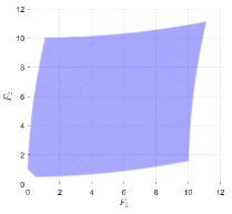
(a) Example 5.1

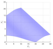
(b) Example 5.2

Figure 1: Visualization of the objective functions $F$ on Examples 5.1 and 5.2.

According to [11, pp. 745], (6) is equivalent to the following optimization problem:

min $$\gamma$$ (23)

s.t. $$\langle\nabla F_{i}(x),u-x\rangle\leq\gamma,~{}i\in\langle m\rangle,$$

$$u\in\Omega.$$

The experiments were conducted using MATLAB R2020b software on a PC with the following specifications: Intel i7-10700 processor running at 2.90 GHz and 32.00 GB RAM. The solver fmincon was employed to solve the subproblem (23). The termination criterion (Step 1 of the CondG algorithm) was set as $\lvert\theta(x^{k})\rvert\leq\epsilon$ with $\epsilon=10^{-6}$. The maximum allowed number of outer iterations was set to 1000. For each test problem, the algorithm was run 100 times with initial points generated from a uniform random distribution within the respective feasible region.

Table 1 presents the results obtained by the algorithm, organized into columns labeled “it”, “gE”, “T” and “%.” The “it” column represents the average number of iterations, while “gE” stands for the average number of gradient evaluations. The “T” column indicates the average computational time (in seconds) to reach the critical point from an initial point, and “%” indicates the percentage of runs that have reached a critical point. As observed in Table 1, the algorithm can effectively solve the two given problems.

Table 1: Performance of the algorithm on the two problems.

	it	gE	T	%
Example 1	18.78	19.78	0.05	100
Example 2	14.81	15.81	0.04	100

To observe the movement of iteration points, we depict the trajectories of these points in Fig. 2. In this figure, dashed lines represent the paths of algorithm iterations, blue points are the initial points, and red points correspond to the solutions found by the algorithm.

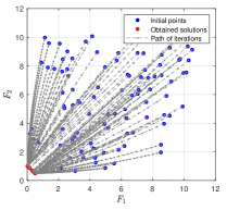
(a) Example 5.1

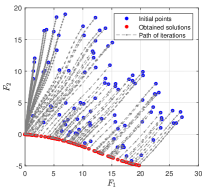
(b) Example 5.2

Figure 2: The final solutions and the paths of iterations obtained by the algorithm on the two examples.

References

References

[1] G.P. Rangaiah, A. Bonilla-Petriciolet, Multi-Objective Optimization in Chemical Engineering: Developments and Applications, John Wiley & Sons, 2013.
[2] C. Zopounidis, E. Galariotis, M. Doumpos, S. Sarri, K. Andriosopoulos, Multiple criteria decision aiding for finance: An updated bibliographic survey, Eur. J. Oper. Res. 247(2) (2015) 339–348.
[3] J. Fliege, OLAF-a general modeling system to evaluate and optimize the location of an air polluting facility, OR Spektrum. 23(1) (2001) 117–136.
[4] M. Tavana, M.A. Sodenkamp, L. Suhl, A soft multi-criteria decision analysis model with application to the European Union enlargement. Ann. Oper. Res. 181(1) (2010) 393–421.
[6] Sener O, Koltun V. Multi-task learning as multi-objective optimization, Adv. Neural Inf. Process. Syst. (2018) 525–536.
[7] J. Fliege, B.F. Svaiter, Steepest descent methods for multicriteria optimization, Math. Methods Oper. Res. 51 (2000) 479–494.
[8] J. Fliege, L.M. Graa Drummond, B.F. Svaiter, Newton’s method for multiobjective optimization, SIAM J. Optim. 20 (2009) 602–626.
[9] L.R. Lucambio Pérez, L.F. Prudente, Nonlinear conjugate gradient methods for vector optimization, SIAM J. Optim. 28(3) (2018) 2690–2720.
[10] M. Lapucci, P. Mansueto, A limited memory Quasi-Newton approach for multi-objective optimization, Comput. Optim. Appl. 85(1) (2023) 33–73.
[11] P.B. Assunção, O.P. Ferreira, L.F. Prudente, Conditional gradient method for multiobjective optimization, Comput. Optim. Appl. 78(3) (2021) 741–768.
[12] W. Chen, X.M. Yang, Y. Zhao, Conditional gradient for vector optimization, Comput. Optim. Appl. 85(1) (2023) 857–896.
[13] J.G. Lin, On min-norm and min-max methods of multi-objective optimization, Math. Program. 103(1) (2005) 1–33.
[14] T.N. Hoa, N.Q. Huy, T.D. Phuong, N.D. Yen, Unbounded components in the solution sets of strictly quasiconcave vector maximization problems, J. Global Optim. 37 (2007) 1–10.
[15] L. Li, J. Li, Equivalence and existence of weak Pareto optima for multiobjective optimization problems with cone constraints, Appl. Math. Lett. 21(6) (2008) 599–606.
[16] N.T.T. Huong, J.C. Yao, N.D. Yen, Geoffrion’s proper efficiency in linear fractional vector optimization with unbounded constraint sets, J. Global Optim. 78(3) (2020) 545–562.
[18] G. Kováčová, B. Rudloff, Convex projection and convex multi-objective optimization, J. Global Optim. 83(2) (2022) 301.-327.
[19] A. Wagner, F. Ulus, B. Rudloff, G. Kováčová, N. Hey, Algorithms to solve unbounded convex vector optimization problems, SIAM J. Optim. 33(4) (2023) 2598–2624.
[20] R.T. Rockafellar, R. Wets, Variational Analysis, Springer, Berlin, 1998.
[21] J. John, Vector Optimization: Theory, Applications and Extensions, 2nd ed. Springer, Berlin, 2011.
[22] K. Miettinen, Nonlinear multiobjective Optimization, Springer Science & Business Media, 1999.
[23] A. Beck, First-order methods in optimization, Society for Industrial and Applied Mathematics, 2017.
[24] L.Y. Zeng, Y.H. Dai, Y.K. Huang, Convergence rate of gradient descent method for multi-objective optimization, J. Comput. Math. 37(5) (2019) 689–703.