Restricted Isometry Property of Rank-One Measurements with Random Unit-Modulus Vectors

Abstract

The restricted isometry property (RIP) is essential for the linear map to guarantee the successful recovery of low-rank matrices. The existing works show that the linear map generated by the measurement matrices with independent and identically distributed (i.i.d.) entries satisfies RIP with high probability. However, when dealing with non-i.i.d. measurement matrices, such as the rank-one measurements, the RIP compliance may not be guaranteed. In this paper, we show that the RIP can still be achieved with high probability, when the rank-one measurement matrix is constructed by the random unit-modulus vectors. Compared to the existing works, we first address the challenge of establishing RIP for the linear map in non-i.i.d. scenarios. As validated in the experiments, this linear map is memory-efficient, and not only satisfies the RIP but also exhibits similar recovery performance of the low-rank matrices to that of conventional i.i.d. measurement matrices.

1 Introduction

The low-rank matrix recovery is a popular topic in many fields, such as wireless communication, signal processing, and image processing (Candes et al., 2013; Chen et al., 2015; Shechtman et al., 2015; Davenport and Romberg, 2016; Zhang et al., 2018b; Chen and Chi, 2018; Chi et al., 2019; Zhang et al., 2019; Zhang and Tay, 2021; Farias et al., 2022; Tong et al., 2022). The primary objective for this problem is to reconstruct a low-rank matrix from a limited number of observations. These observations are obtained through a linear map, which consists of the measurement matrices. To be more specific, the measurements for a low-rank matrix $\mathbf{X}\in{\mathbb{C}}^{M\times N}$ are give by the following

$$y_{k} =\frac{1}{\sqrt{K}}\langle\mathbf{A}_{k},\mathbf{X}\rangle+z_{k},k=1,2,\ldots,K,$$ (1)

where $\mathbf{A}_{k}\in{\mathbb{C}}^{M\times N}$ are the measurement matrices, $\langle\mathbf{A}_{k},\mathbf{X}\rangle=\operatorname{tr}(\mathbf{A}_{k}^{H}\mathbf{X})$, and $z_{k}$ is the noise or measurement error. The $K$ measurement matrices $\{\mathbf{A}_{k}\}_{k=1}^{K}$ collectively define a linear map, denoted as $\mathcal{A}(\cdot):\mathbb{C}^{M\times N}\rightarrow\mathbb{C}^{K\times 1}$, where each entry of ${\mathcal{A}}(\mathbf{X})$ is given by $[{\mathcal{A}}(\mathbf{X})]_{k}=\frac{1}{\sqrt{K}}\langle\mathbf{A}_{k},\mathbf{X}\rangle,k=1,2,\ldots,K.$ Thus, the measurement model in 1 is shown in a compact form

$$\mathbf{y}={\mathcal{A}}(\mathbf{X})+\mathbf{z},$$ (2)

where $\mathbf{y}=[y_{1},\ldots,y_{K}]^{T}$ and $\mathbf{z}=[z_{1},\ldots,z_{K}]^{T}$.

The goal of low-rank matrix recovery is to reconstruct $\mathbf{X}$ from the linear map ${\mathcal{A}}(\cdot)$ and measurements $\mathbf{y}$ in 2. There are various approaches, including both convex and non-convex methods, (Recht et al., 2010; Candes and Plan, 2011; Chen and Chi, 2018; Chi et al., 2019; Ma et al., 2018; Jain et al., 2013, 2010; Zheng and Lafferty, 2015; Tu et al., 2016) can be utilized to fulfill the goal. The convex methods (Recht et al., 2010; Candes and Plan, 2011; Chen and Chi, 2018) utilize the nuclear norm of $\mathbf{X}$ as a penalty term in their objective functions to promote low-rank solutions. It has been shown that, when the linear map satisfies the restricted isometry property (RIP) with the required RIP constant, these convex methods can guarantee successful recovery in noiseless scenarios or bounded reconstruction errors in the presence of noise. In addition to convex methods, non-convex techniques (Chi et al., 2019; Ma et al., 2018; Jain et al., 2013, 2010; Zheng and Lafferty, 2015; Tu et al., 2016), such as gradient-based methods and alternating minimization methods, offer greater computational efficiency . Notably, these gradient-based methods, as demonstrated in the works by Chi et al. (2019); Zheng and Lafferty (2015); Tu et al. (2016), can ensure convergence with proper initialization when the linear map $\mathcal{A}(\cdot)$ satisfies the RIP with the necessary constant. Furthermore, some studies (Ge et al., 2017; Zhang et al., 2018a) have investigated the presence of spurious local minima in low-rank matrix recovery problems. When there are no spurious local minima, non-convex methods can achieve global minima. The works by Ge et al. (2017); Zhang et al. (2018a) have shown that, when the linear map ${\mathcal{A}}(\cdot)$ satisfies the RIP with the required constant, the low-rank matrix recovery problem formulated in this manner has no spurious local minima, thereby guaranteeing exact recovery.

As mentioned above, one can find that the RIP of the linear map ${\mathcal{A}}(\cdot)$ plays an important role in ensuring the low-rank matrix recovery. In particular, the definition of RIP is presented below.

Definition 1 (Standard RIP over Low-Rank Matrices (Candes and Plan, 2011)).

For the set of rank-$r$ matrices, we define the RIP constant $\delta_{r}$with respect to operator ${\mathcal{A}}(\cdot)$ as the smallest numbers such that for all $\mathbf{X}$ of rank at most $r$:

$$(1-\delta_{r})\|\mathbf{X}\|_{F}^{2}\leq\|{\mathcal{A}}(\mathbf{X})\|_{2}^{2}\leq(1+\delta_{r})\|\mathbf{X}\|_{F}^{2}.$$

There are many types of linear map that satisfy the defined RIP above. When the entries of $\mathbf{A}_{k}$ are i.i.d. complex Gaussian entries (Recht et al., 2010; Candes and Plan, 2011), or when the entries of $\mathbf{A}_{k}$ are i.i.d. unit-modulus (Zhang et al., 2018b), where each entry is unit-modulus and its phase follows a uniform distribution in the range $[0,2\pi]$, then the linear map ${\mathcal{A}}(\cdot)$ satisfies the RIP with high probability, on the condition that the number of measurements $K\geq c(M+N)r$ for large enough constant $c>0$.

However, in certain scenarios of low-rank matrix recovery, the entries in the measurement matrix are non-i.i.d. or do not follow the distributions mentioned above, such as the low-rank matrix completion (Candès and Recht, 2009; Candès and Tao, 2010), phase retrieval (Candes et al., 2015; Ma et al., 2018), and quadratic sensing problem (Chen et al., 2015; Cai and Zhang, 2015). In general, the associated linear map $\mathcal{A(\cdot)}$ in these scenarios does not satisfy the RIP property. To analyze the recovery performance guarantee under these non-RIP scenarios, some variants of RIP are defined, such as incoherence for matrix completion (Candès and Recht, 2009; Candès and Tao, 2010) and RIP-$\ell_{2}/\ell_{1}$ for the rank-one measurements (Chen et al., 2015; Cai and Zhang, 2015). However, many existing advancements based on RIP, such as the works in (Chi et al., 2019; Ma et al., 2018; Jain et al., 2013, 2010; Zheng and Lafferty, 2015; Tu et al., 2016) , are not applicable for these non-RIP scenarios.

In this paper, our primary focus is on the concept of rank-one measurements as introduced by Cai and Zhang (2015). We aim to demonstrate that when the measurement matrix follows the specified distribution, the associated linear map satisfies the RIP. It is worth noting that the quadratic sensing problem and phase retrieval can be considered special cases of the rank-one projection problem. For rank-one measurements (Cai and Zhang, 2015; Li et al., 2019), the measurement matrix $\mathbf{A}_{k}$ can be represented as an outer product of two vectors,

$$\mathbf{A}_{k} =\mathbf{u}^{H}_{k}\mathbf{v}_{k}.$$ (3)

However, in general cases where the measurement matrices $\mathbf{A}_{k}$ are defined above, it has been established in prior works (Cai and Zhang, 2015; Chi et al., 2019) that the associated linear map does not satisfy the RIP. For example, studies of Chi et al. (2019); Cai and Zhang (2015); Chen et al. (2015) have shown that when the entries of both $\mathbf{u}_{k}$ and $\mathbf{v}_{k}$ are i.i.d. Gaussian, the associated linear map $\mathcal{A(\cdot)}$ does not satisfy the RIP. In our work, we impose specific distribution on the random vectors $\mathbf{u}_{k}$ and $\mathbf{v}_{k}$ instead of i.i.d. Gaussian in the existing works (Chi et al., 2019; Cai and Zhang, 2015; Chen et al., 2015). We show that when the entries in $\mathbf{u}_{k}$ and $\mathbf{v}_{k}$ are i.i.d. unit-modulus, the associated linear map satisfies the RIP with high probability. As far as we know, our research marks the first attempt to tackle the challenge of establishing RIP for the linear map in non-i.i.d. scenarios. Additionally, it lays the foundational framework for proving RIP in various forms of random rank-one measurements.

2 RIP Analysis of Linear Map

2.1 Sufficient Condition of RIP

For arbitrary $\mathbf{u}_{k}$ and $\mathbf{v}_{k}$ in 3, whether the corresponding linear map ${\mathcal{A}}(\cdot)$ satisfies the RIP is challenging to check. Fortunately, the following theorem provides a sufficient condition on which the linear map ${\mathcal{A}}(\cdot)$ satisfies the RIP.

Theorem 1 (Candes and Plan (2011), Theorem 2.3).

Let ${\mathcal{A}}(\cdot):{\mathbb{C}}^{M\times N}\rightarrow{\mathbb{C}}^{K\times 1}$ be a linear map with random measurement matrices obeying the following condition: for any given $\mathbf{X}\in{\mathbb{C}}^{M\times N}$ and any fixed $0<\alpha<1$

$$\!\!\Pr\left(\left|\|{\mathcal{A}}(\mathbf{X})\|_{2}^{2}-\|\mathbf{X}\|_{F}^{2}\right|\!\geq\!\alpha\|\mathbf{X}\|_{F}^{2}\right)\leq C\exp(-cK)$$ (4)

for fixed constants $C,c>0$ (which may depend on $\alpha$). Then if $K\geq D\max\{M,N\}r$, ${\mathcal{A}}$ satisfies the RIP with constant $\delta_{r}>0$ with probability exceeding $1-Ce^{-dK}$ for fixed constants $D,d>0$.

Without loss of generality, we assume $\|\mathbf{X}\|_{F}=1$. Therefore, according to Theorem 1, in order to show the linear map ${\mathcal{A}}(\cdot)$ meet RIP, we need to prove the following probability

$$\Pr\left(\left|\|{\mathcal{A}}(\mathbf{X})\|_{2}^{2}-1\right|\geq\alpha\right)$$ (5)

is close to zero. Note that the probability is taken over the linear map ${\mathcal{A}}(\cdot)$ and the $\mathbf{X}$ is fixed and arbitrary.

For the linear map ${\mathcal{A}}(\cdot)$ where the entries in $\mathbf{A}_{k}$ are drawn from i.i.d. ${\mathcal{C}}{\mathcal{N}}(0,1)$, it is easy to verify that the condition in 4 holds. Therefore, the corresponding linear map satisfies the RIP with high probability. This is also consistent with the real case where $\mathbf{A}_{k}$ are drawn according to i.i.d. ${\mathcal{N}}(0,1)$ in the following.

Remark 1 (Recht et al. (2010); Candes and Plan (2011)).

If the entries of $\mathbf{A}_{k}$ are i.i.d. Gaussian entries ${\mathcal{N}}(0,1)$, then ${\mathcal{A}}(\cdot)$ satisfies the $r$-RIP with RIP constant $\delta_{r}$ with high probability as $K\gtrsim(M+N)r/\delta_{r}^{2}$.

Moreover, when the entries in $\mathbf{A}_{k}$ of the linear map are i.i.d. (Recht et al., 2010; Candes and Plan, 2011; Zhang et al., 2018b) , the central limit theorem can be applied to approximately verify the sufficient condition in 4. However, for the rank-one model in 3, the entries of measurement matrix $\mathbf{A}_{k}$ are dependent. Due to this dependence, the standard RIP in Definition 1 may not hold for the general $\mathbf{u}_{k}$ and $\mathbf{v}_{k}$. For example, when the entries of $\mathbf{u}_{k}$ and $\mathbf{v}_{k}$ are i.i.d. Gaussian, the RIP does not hold in this scenario because the $\mathbf{u}^{H}\mathbf{X}\mathbf{v}$ involves fourth moments of Gaussian variable (Cai and Zhang, 2015; Kueng et al., 2017; Candes et al., 2013).

To evaluate the concentration property of the linear map for this dependent and rank-one measurement model in 3, some alternative conditions, such as RIP-$\ell_{1}/\ell_{1}$ (Candes et al., 2013) and RIP-$\ell_{2}/\ell_{1}$ (Chen et al., 2015; Cai and Zhang, 2015), have been proposed. These studies demonstrate that the convex methods can ensure the exact recovery based on these alternative conditions. However, in the context of non-convex analyses, techniques like the alternating minimization method (Jain et al., 2013), singular value projection method (Jain et al., 2010), and other local optimal analysis (Ge et al., 2017; Chi et al., 2019; Ma et al., 2018), these variants of RIP (Candes et al., 2013; Chen et al., 2015; Cai and Zhang, 2015) are not applicable, because these analysis are based on the standard RIP. Thus, this highlights the crucial importance of standard RIP in Definition 1 compared to its variants.

It is indeed a well-established fact that the linear map ${\mathcal{A}}(\cdot)$ with general setting for $\mathbf{u}_{k}$ and $\mathbf{v}_{k}$ in 3 may not satisfy the standard RIP. However, in this paper, we find that if we impose some specific design for $\mathbf{u}_{k}$ and $\mathbf{v}_{k}$, it becomes possible to attain the standard RIP for the designed linear map. The main result of the paper is presented in the following theorem.

Theorem 2.

If the measurement matrix $\mathbf{A}_{k}=\mathbf{u}_{k}^{H}\mathbf{v}^{k}\in{\mathbb{C}}^{M\times N}$, where $\mathbf{u}_{k}\in{\mathbb{C}}^{M\times 1},\mathbf{v}_{k}\in{\mathbb{C}}^{N\times 1}$ are given in the following

$$\mathbf{u}_{k} =[e^{j\theta_{k,1}},\ldots,e^{j\theta_{k,M}}]^{T},$$

$$\mathbf{v}_{k} =[e^{j\phi_{k,1}},\ldots,e^{j\phi_{k,N}}]^{T},$$ (6)

with $\theta_{k,m},\forall\,m$ and $\phi_{k,n},\forall\,n$ being i.i.d. from a uniform distribution on $[0,2\pi]$. For the linear map ${\mathcal{A}}(\cdot):{\mathbb{C}}^{M\times N}\rightarrow{\mathbb{C}}^{K\times 1}$ generated by $\{\mathbf{A}_{k}\}_{k=1}^{K}$, where

$$[{\mathcal{A}}(\mathbf{X})]_{k} =\frac{1}{\sqrt{K}}\langle\mathbf{A}_{k},\mathbf{X}\rangle,$$

$$=\frac{1}{\sqrt{K}}\mathbf{u}_{k}^{H}\mathbf{X}\mathbf{v}_{k},\forall\,k=1,2,\ldots,K,$$

it satisfies RIP with high probability as long as $K\geq D(M+N)r$ for some large enough constant $D$.

Intuitively, the reason that the standard RIP for the linear map 6 holds is because the entries in $\mathbf{u}_{k}$ and $\mathbf{v}_{k}$ are unit-modulus, which are bounded compared to the scenario where $\mathbf{u}_{k}$ and $\mathbf{v}_{k}$ are i.i.d. Gaussian (Chen et al., 2015; Cai and Zhang, 2015). Moreover, they experience some special symmetric statistical property compared to i.i.d. Gaussian scenario, which enables us to prove the RIP in the following sections. Before delving into details of the proof, we first discuss the applications of the measurement model outlined in 6.

Compared to the i.i.d. measurement matrix $\mathbf{A}_{k}$, the rank-one measurements can offer enhanced storage efficiency for the linear map, as demonstrated by (Cai and Zhang, 2015). Moreover, within the context of rank-one measurements, the designed unit-modulus setting in 6 can further save the storage of the measurement matrices, as opposed to case of i.i.d. Gaussian $\mathbf{u}_{k}$ and $\mathbf{v}_{k}$. The reason behind this efficiency is that, for the unit-modulus setting described in 6, it is necessary to store only the phases of the vectors $\mathbf{u}_{k}$ and $\mathbf{v}_{k}$. In contrast, for the i.i.d. Gaussian $\mathbf{u}_{k}$ and $\mathbf{v}_{k}$, one must preserve both the magnitudes and phases of these vectors to accurately construct the measurement matrix $\mathbf{A}_{k}$. Most importantly, based on the established results in Theorem 2, the proposed unit-modulus rank-one measurements are applicable for many RIP-based algorithms or analysis (Jain et al., 2013, 2010; Ge et al., 2017; Chi et al., 2019; Ma et al., 2018), making the rank-one unit-modulus measurements a promising option for the matrix recovery task. Therefore, building on the advantages highlighted earlier, the rank-one measurement model with unit-modulus vectors in 6 has widespread applications in the field of low-rank matrix recovery, especially when the configuration of the measurement matrices is applicable, such as channel estimation in communication systems (El Ayach et al., 2014; Zhang et al., 2018b, 2020), phase retrieval (Candes et al., 2013; Ma et al., 2018), covariance estimation (Chen et al., 2015), and X-ray crystallography (Shechtman et al., 2015).

2.2 Inequalities of Tail Bounds

To establish the fact that the linear map in Theorem 2 satisfies the RIP, we need to evaluate the probability of the event in 5. After straightforward manipulations, one can find that ${\mathbb{E}}[\|\mathbf{y}\|_{2}^{2}]=1$. Thus, the bound in 5 is about the tail bound. When the probability is small, it means that the value of $\|\mathbf{y}\|_{2}^{2}$ is strictly concentrated around its expected value. In the following, we will evaluate the upper and lower tail bounds, respectively.

For the upper tail bound, due to the independence among the entries of ${\mathcal{A}}(\mathbf{X})$, one can apply Chernoff bound for any $h>0$,

$$\Pr(\|{\mathcal{A}}(\mathbf{X})\|_{2}^{2}\geq(1+\alpha)) =\Pr(hK\|{\mathcal{A}}(\mathbf{X})\|_{2}^{2}\geq hK(1+\alpha))$$

$$=\Pr(e^{hK\|{\mathcal{A}}(\mathbf{X})\|_{2}^{2}}\geq e^{hK(1+\alpha)})$$

$$\leq{\mathbb{E}}[e^{hK\|{\mathcal{A}}(\mathbf{X})\|_{2}^{2}}]e^{-hK(1+\alpha)}.$$

Since the second part of the right-hand side (R.H.S.) of the inequality above, i.e., $e^{-hK(1+\alpha)}$, goes to zero as $K$ goes to infinity, we focus on the first part,

$${\mathbb{E}}[e^{hK\|{\mathcal{A}}(\mathbf{X})\|_{2}^{2})}] ={\mathbb{E}}[e^{h\sum_{k=1}{|\langle\mathbf{A}_{k},\mathbf{X}\rangle|^{2}}}]$$

$$=\left({\mathbb{E}}[e^{h{|\langle\mathbf{A}_{1},\mathbf{X}\rangle|^{2}}}]\right)^{K}$$

$$=\left({\mathbb{E}}[e^{{h}{|\mathbf{u}_{1}^{H}\mathbf{X}\mathbf{v}_{1}|^{2}}}]\right)^{K}.$$

For convenience, we ignore the subscript the subscripts of $\mathbf{u}$ and $\mathbf{v}$. Using Taylor series for $e^{hK{|\langle\mathbf{A}_{1},\mathbf{X}\rangle|^{2}}}$ gives

$${\mathbb{E}}[e^{{h}{|\mathbf{u}^{H}\mathbf{X}\mathbf{v}|^{2}}}] ={\mathbb{E}}\left[\sum_{t=0}^{\infty}\frac{h^{t}}{t!}|\mathbf{u}^{H}\mathbf{X}\mathbf{v}|^{2t}\right]$$

$$=\sum_{t=0}^{\infty}\frac{h^{t}}{t!}{\mathbb{E}}[|\mathbf{u}^{H}\mathbf{X}\mathbf{v}|^{2t}].$$ (7)

For the lower tail bound in 5, we have

$$\Pr(\|{\mathcal{A}}(\mathbf{X})\|_{2}^{2}\leq(1-\alpha)) =\Pr(-hK\|{\mathcal{A}}(\mathbf{X})\|_{2}^{2}\geq-hK(1-\alpha))$$

$$\leq{\mathbb{E}}[e^{-hK\|{\mathcal{A}}(\mathbf{X})\|_{2}^{2}}]e^{hK(1-\alpha)}$$

$$=\left({\mathbb{E}}[e^{-h{|\mathbf{u}^{H}\mathbf{X}\mathbf{v}|^{2}}}]\right)^{K}e^{hK(1-\alpha)}.$$

Similarly, using the Taylor series yields

$${\mathbb{E}}[e^{-h{|\mathbf{u}^{H}\mathbf{X}\mathbf{v}|^{2}}}] ={\mathbb{E}}\left[\sum_{t=0}^{\infty}\frac{(-h)^{t}}{t!}|\mathbf{u}^{H}\mathbf{X}\mathbf{v}|^{2t}\right]$$

$$=\sum_{t=0}^{\infty}\frac{(-h)^{t}}{t!}{\mathbb{E}}[|\mathbf{u}^{H}\mathbf{X}\mathbf{v}|^{2t}].$$ (8)

In summary, we have the following upper tail probability bound

$$\Pr(\|{\mathcal{A}}(\mathbf{X})\|_{2}^{2}\geq(1+\alpha))\leq\left(\sum_{t=0}^{\infty}\frac{h^{t}}{t!}{\mathbb{E}}[|\mathbf{u}^{H}\mathbf{X}\mathbf{v}|^{2t}]\right)^{K}e^{-hK(1+\alpha)},$$ (9)

and the lower tail probability bound

$$\Pr(\|{\mathcal{A}}(\mathbf{X})\|_{2}^{2}\leq(1-\alpha))\leq\left(\sum_{t=0}^{\infty}\frac{(-h)^{t}}{t!}{\mathbb{E}}[|\mathbf{u}^{H}\mathbf{X}\mathbf{v}|^{2t}]\right)^{K}e^{hK(1-\alpha)}.$$ (10)

To check whether the sufficient condition in 4 holds for the linear map ${\mathcal{A}}(\cdot)$, we need to evaluate the values in 9 and 10. By observing the R.H.S. of 9 and 10, one can find that the key is to calculate ${\mathbb{E}}[|\mathbf{u}^{H}\mathbf{X}\mathbf{v}|^{2t}]$.

3 Connection with the All-One Matrix

The value of ${\mathbb{E}}[|\mathbf{u}^{H}\mathbf{X}\mathbf{v}|^{2t}]$ depends on the realizations of $\mathbf{X}$, which is challenging to manipulate. To handle this, we first focus on a specific $\mathbf{X}$, where $\mathbf{X}=\frac{1}{\sqrt{MN}}\bm{1}\bm{1}^{T}$, then establish a relationship between ${\mathbb{E}}[|\mathbf{u}^{H}\mathbf{X}\mathbf{v}|^{2t}]$ and ${\mathbb{E}}[|\mathbf{u}^{H}\bm{1}\bm{1}^{T}\mathbf{v}|^{2t}]$. In particular, when $\mathbf{X}=\frac{1}{\sqrt{MN}}\bm{1}\bm{1}^{T}$, we have that

$${\mathbb{E}}\left[\left|\mathbf{u}^{H}\frac{1}{\sqrt{MN}}\bm{1}\bm{1}^{T}\mathbf{v}\right|^{2t}\right]=\frac{1}{M^{t}N^{t}}{\mathbb{E}}\left[\left|\sum_{m=1}\mathbf{u}_{m}^{*}\right|^{2t}\right]{\mathbb{E}}\left[\left|\sum_{n=1}\mathbf{v}_{n}\right|^{2t}\right].$$ (11)

Compared to ${\mathbb{E}}[|\mathbf{u}^{H}\mathbf{X}\mathbf{v}|^{2t}]$, the value in 11 only depends on the random vector $\mathbf{u}$ and $\mathbf{v}$, which is applicable to derive a bound for it. We first provide some preliminaries, and all their proofs are attached in Section B of the supplementary materials.

First of all, the following lemma is about the maximization of summation of combinations.

Lemma 1.

Suppose $0\leq p\leq 1$ and $n\geq 0$, the summation below

$$s_{n}(p)=\sum_{k=0}^{n}\binom{n}{k}^{2}p^{k}(1-p)^{n-k}$$

is maximized when $p=1/2$.

Since the summation term $p+(1-p)=1$, the Lemma 1 shows that the average value, i.e., $p=1/2$, achieves the maximum of $s_{n}(p)$. The results in Lemma 1 will be utilized to compare the value of ${\mathbb{E}}[|\mathbf{u}^{H}\mathbf{X}\mathbf{v}|^{2t}]$ with ${\mathbb{E}}[|\mathbf{u}^{H}\bm{1}\bm{1}^{T}\mathbf{v}|^{2t}]$. As a straightforward extension, when $p+(T-p)=T$, the following Corollary holds.

Corollary 1.

Suppose $0\leq p\leq T$ and $n\geq 0$, the summation below

$$s_{n}(p)=\sum_{k=0}^{n}\binom{n}{k}^{2}p^{k}(T-p)^{n-k}$$

is maximized when $p=0.5T$.

Before comparing the values of ${\mathbb{E}}[|\mathbf{u}^{H}\mathbf{X}\mathbf{v}|^{2t}]$ and ${\mathbb{E}}[|\mathbf{u}^{H}\bm{1}\bm{1}^{T}\mathbf{v}|^{2t}]$, we start from the simplified case where $\mathbf{x}\in{\mathbb{C}}^{N\times 1}$ and disregard the vector $\mathbf{u}$. Specifically, we evaluate the values of ${\mathbb{E}}\left[|\mathbf{x}^{T}\mathbf{v}|^{2m}\right]$ and ${\mathbb{E}}\left[|\bm{1}^{T}\mathbf{v}|^{2m}\right],\forall\,m$. By doing so, we lay the foundation for extending these findings to a more general settingby incorporating additional considerations

Theorem 3.

Suppose $\mathbf{v}=[e^{j\phi_{1}},\ldots,e^{j\phi_{N}}]^{T}$ with $\phi_{n},\forall\,n$ being i.i.d. from a uniform distribution on $[0,2\pi]$. If $\mathbf{x}\in{\mathbb{C}}^{N\times 1}$ with $\|\mathbf{x}\|_{2}=1$, then for any $m\geq 0$, ${\mathbb{E}}\left[|\mathbf{x}^{T}\mathbf{v}|^{2m}\right]$ is maximized when $x_{n}=\frac{1}{\sqrt{N}},\forall\,n$.

Thus, according to Theorem 3, for any $\|\mathbf{x}\|_{2}=1$, one has the following inequality,

$${\mathbb{E}}[|\mathbf{x}^{T}\mathbf{v}|^{2m}]\leq\frac{1}{N^{m}}{\mathbb{E}}[|\bm{1}^{T}\mathbf{v}|^{2m}],\forall\,m.$$

Furthermore, in order to extend the vector-case results in Theorem 3 to a more general setting, we need the following Lemmas 2, 3 and 4 as preliminaries.

Lemma 2.

Suppose $t>0$ and $k_{m}\geq 0$ are integers, and non-negative $c_{m}\in{\mathbb{R}},\forall\,m=1,2,\ldots,M$, with $\sum_{m=1}^{M}c_{m}^{2}=1$, then the following holds

$$\sum_{k_{1}+\ldots+k_{M}=t}{\binom{t}{k_{1},\ldots,k_{M}}}^{2}\prod_{m=1}^{M}c_{m}^{2k_{m}}\leq\sum_{k_{1}+\ldots+k_{M}=t}M^{-t}{\binom{t}{k_{1},\ldots,k_{M}}}^{2},$$ (12)

where the equality holds when $c_{m}=1/\sqrt{M}$.

The results in Lemma 2 mean that the summation about the combinatorial expression is maximized when the values of $c_{m},\forall\,m,$ are equivalent, which is the extension of result in the one-variable case of Corollary 1.

Lemma 3.

Suppose non-negative random variables $X_{1},X_{2}$, for any $k_{1},k_{2}\geq 0$ and $1/p+1/q=1$ with $p,q\in[1,+\infty)$, then we have

$${\mathbb{E}}\left[X_{1}^{k_{1}}X_{2}^{k_{2}}\right] \leq({\mathbb{E}}[X_{1}^{k_{1}p}])^{1/p}({\mathbb{E}}[X_{2}^{k_{2}q}])^{1/q}.$$ (13)

In particular,

$${\mathbb{E}}[X_{1}^{k_{1}}X_{2}^{k_{2}}] \leq\max\{{\mathbb{E}}[X_{1}^{k_{1}+k_{2}}],{\mathbb{E}}[X_{2}^{k_{1}+k_{2}}]\}.$$ (14)

The results in Lemma 3 are to bound ${\mathbb{E}}[X_{1}^{k_{1}}X_{2}^{k_{2}}]$ by the product of expectations, where the latter is more applicable to handle. Then, the following lemma is an extension of the results in Lemma 3, where there are $N$ random variables.

Lemma 4.

Suppose non-negative random variables $X_{1},X_{2},\ldots,X_{N}$, for any $k_{n}\geq 0$, then the following inequality about expectation holds

$${\mathbb{E}}\left[\prod_{n=1}^{N}X_{n}^{k_{n}}\right] \leq\prod_{n=1}^{N}\left({\mathbb{E}}\left[X_{n}^{t}\right]\right)^{k_{n}/t}$$

$$\leq\max_{n}{\mathbb{E}}\left[X_{n}^{t}\right],$$ (15)

where $t=\sum_{n=1}^{N}k_{n}$.

With the results in Lemmas 2, 3 and 4, we are now ready to compare the values of ${\mathbb{E}}[|\mathbf{u}^{H}\mathbf{X}\mathbf{v}|^{2t}]$ and $\frac{1}{M^{t}N^{t}}{\mathbb{E}}[|\mathbf{u}^{H}\bm{1}\bm{1}^{T}\mathbf{v}|^{2t}]$ in the following theorem, which is proved in Section A of the supplementary materials.

Theorem 4.

For any matrix $\mathbf{X}\in{\mathbb{C}}^{M\times N}$ with $\|\mathbf{X}\|_{F}=1$, the following

$${\mathbb{E}}[|\mathbf{u}^{H}\mathbf{X}\mathbf{v}|^{2t}]\leq\frac{1}{M^{t}N^{t}}{\mathbb{E}}[|\mathbf{u}^{H}\bm{1}\bm{1}^{T}\mathbf{v}|^{2t}]$$

holds for any non-negative integer $t$. Here, $\mathbf{u}\in{\mathbb{C}}^{M\times 1}$ and $\mathbf{v}\in{\mathbb{C}}^{N\times 1}$ are random vectors given by

$$\mathbf{u}=[e^{j\theta_{1}},\ldots,e^{j\theta_{M}}]^{T},~{}\mathbf{v}=[e^{j\phi_{1}},\ldots,e^{j\phi_{N}}]^{T}$$

with $\theta_{m},\forall\,m$ and $\phi_{n},\forall\,n$ being i.i.d in $[0,2\pi]$ .

Thus, the results in Theorem 4 establish a relationship between ${\mathbb{E}}[|\mathbf{u}^{H}\mathbf{X}\mathbf{v}|^{2t}]$ and ${\mathbb{E}}[|\mathbf{u}^{H}\bm{1}\bm{1}^{T}\mathbf{v}|^{2t}]$, where the latter the only depends on the random vector $\mathbf{u}$ and $\mathbf{v}$. Therefore, to further proceed with Theorem 4 and obtain a valid bound for ${\mathbb{E}}[|\mathbf{u}^{H}\mathbf{X}\mathbf{v}|^{2t}]$ in 9 and 10, it necessary to assess the value of ${\mathbb{E}}[|\mathbf{u}^{H}\bm{1}\bm{1}^{T}\mathbf{v}|^{2t}]$. Due to the independence between $\mathbf{u}$ and $\mathbf{v}$, one can express this as ${\mathbb{E}}[|\mathbf{u}^{H}\bm{1}\bm{1}^{T}\mathbf{v}|^{2t}]={\mathbb{E}}[|\mathbf{u}^{H}\bm{1}|^{2t}]{\mathbb{E}}[\bm{1}^{T}\mathbf{v}|^{2t}]$. In this context, the following proposition provides a valuable bound for both ${\mathbb{E}}[|\mathbf{u}^{H}\bm{1}|^{2t}]$ and ${\mathbb{E}}[\bm{1}^{T}\mathbf{v}|^{2t}]$.

Proposition 1.

Since the entries in $\mathbf{u}$ and $\mathbf{v}$ are i.i.d. , one can check that

$${\mathbb{E}}\left[\left|\mathbf{u}^{H}\bm{1}\right|^{2t}\right] ={\mathbb{E}}\left[\left(u_{1}+,\ldots,+u_{M}\right)^{t}\left(u_{1}^{*}+,\ldots,+u_{M}^{*}\right)^{t}\right]$$

$$=\sum_{t_{1}+\ldots+t_{M}=t}{\binom{t}{t_{1},\ldots,t_{M}}}^{2}.$$

One can find that the value above is the number of abelian squares of length $2t$ over an alphabet with $M$ letters (Richmond and Shallit, 2008), denoted as $g(t,M)$. Similarly, the value of ${\mathbb{E}}\left[|\bm{1}^{T}\mathbf{v}|^{2t}\right]$ is given by

$${\mathbb{E}}\left[|\bm{1}^{T}\mathbf{v}|^{2t}\right] =\sum_{t_{1}+\ldots+t_{N}=t}{\binom{t}{t_{1},\ldots,t_{N}}}^{2}$$

$$=g(t,N).$$

Now, the bounds of $g(t,N)$ and $g(t,M)$ are of interest. Based on the results by Richmond and Shallit (2008), the values of $g(t,M)$ and $g(t,N)$ are bounded by

$$g(t,M) \leq C_{1}M^{2t}t^{(1-M)/2},$$

$$g(t,N) \leq C_{2}N^{2t}t^{(1-N)/2},$$

where $C_{1}$ and $C_{2}$ are two constants. Therefore, the value of ${\mathbb{E}}[|\mathbf{u}^{H}\bm{1}\bm{1}^{T}\mathbf{v}/{\sqrt{MN}}|^{2t}]$ is upper bounded by

$${\mathbb{E}}\left[\left|\mathbf{u}^{H}\frac{\bm{1}\bm{1}^{T}}{\sqrt{MN}}\mathbf{v}\right|^{2t}\right]\leq CM^{t}N^{t}t^{1-\frac{M+N}{2}},$$ (16)

where $C=C_{1}C_{2}$ is a constant.

4 RIP of Rank-One Unit-Modulus Measurements

In this section, we prove the RIP of rank-one measurements with unit-modulus vectors in Theorem 2. Recall that it is essential to evaluate the bounds in 9 and 10 to show they satisfy the sufficient condition in Theorem 1. Based on the established results in Section 3, we can simplify the upper and lower tail bounds in 9 and 10, respectively, as shown in the following theorem.

Theorem 5.

For the linear map ${\mathcal{A}}(\cdot)$ defined in Theorem 2, we have the following upper tail probability bound for any $\mathbf{X}\in{\mathbb{C}}^{M\times N}$ with $\|\mathbf{X}\|_{F}=1$,

$$\Pr(\|{\mathcal{A}}(\mathbf{X})\|_{2}^{2}\geq(1+\alpha))\leq e^{-c_{1}K},$$ (17)

where $c_{1}>0$ is a constant depending on $\alpha$. In addition, the lower tail probability bound is given by

$$\Pr(\|{\mathcal{A}}(\mathbf{X})\|_{2}^{2}\leq(1-\alpha))\leq e^{-c_{2}K},$$ (18)

where $c_{2}>0$ is also a constant depending on $\alpha$.

According to the results in Theorem 5, it is evident that both the upper and lower tail bounds exhibit an exponential decrease as the number of measurements $K$. This observation leads us to verify the sufficient condition for the RIP outlined in Theorem 1. Consequently, the linear map associated with random unit-modulus vectors satisfies the RIP with high probability, as shown in Theorem 2. In the following, we provide a comprehensive proof of Theorem 5.

Proof of Theorem 5. To prove the upper tail bound in 17, we combine the results in 9 and Theorem 4,

$$\Pr(\|{\mathcal{A}}(\mathbf{X})\|_{2}^{2}\geq(1+\alpha)) \leq\left(\sum_{t=0}^{\infty}\frac{h^{t}}{t!}{\mathbb{E}}[|\mathbf{u}^{H}\mathbf{X}\mathbf{v}|^{2t}]\right)^{K}e^{-hK(1+\alpha)}$$

$$\leq\left(\sum_{t=0}^{\infty}\frac{h^{t}}{t!}{\mathbb{E}}\left[\left|\mathbf{u}^{H}\frac{\bm{1}\bm{1}^{T}}{\sqrt{MN}}\mathbf{v}\right|^{2t}\right]\right)^{K}e^{-hK(1+\alpha)}.$$

Then from Proposition 1, we have

$$\Pr(\|{\mathcal{A}}(\mathbf{X})\|_{2}^{2}\geq(1+\alpha))$$

$${\leq}\Bigg{(}1+h+2h^{2}-\frac{2M+2N-1}{2MN}h^{2}+\sum_{t=3}^{\infty}\frac{h^{t}}{t!}CM^{t}N^{t}t^{1-\frac{M+N}{2}}\Bigg{)}^{K}e^{-hK(1+\alpha)}.$$ (19)

In the following, we need to choose a $h$ which makes the bound above tight. Note that there exists $Z>0$, which makes the following hold for any $0<h\leq Z\alpha$,

$$1+h+2h^{2}-\frac{2M+2N-1}{2MN}h^{2}+\sum_{t=3}^{\infty}\frac{h^{t}}{t!}CM^{t}N^{t}t^{1-\frac{M+N}{2}}\leq 1+h+2h^{2}.$$ (20)

For convenience, we define

$$f(h)=(1+h+2h^{2})e^{-h(1+\alpha)}.$$

Thus, according to 19 and 20, for any $0<h\leq Z\alpha$, the tail probability in 19 is bounded as follows

$$\Pr(\|{\mathcal{A}}(\mathbf{X})\|_{2}^{2}\geq(1+\alpha))\leq(f(h))^{K}.$$ (21)

Comparing 21 with the sufficient condition in 4, we need to prove that the above expression has the form of $C\exp(-cK)$. In other words, we need to show there exists a $h_{1}\in(0,Z\alpha]$ such that $f(h_{1})<1$, then $(f(h_{1}))^{K}$ converges to zero as $K$ goes to infinity.

Note that $f(0)=1$. Thus, in order to show there exists $h_{1}$ such that $f(h_{1})<1$, it is sufficient to show the first derivative of $f$ at $0$ is negative, i.e., $f^{\prime}(0)<0$, which is obviously true. Therefore, we choose $h=h_{1}$, the expression in 21 is rewritten as

$$\Pr(\|{\mathcal{A}}(\mathbf{X})\|_{2}^{2}\geq(1+\alpha)) \leq(1+h_{1}+2h_{1}^{2})^{K}e^{-h_{1}K(1+\alpha)}$$

$$=e^{-c_{1}K},$$

where the constant $c_{1}=-\ln(f(h_{1}))=-\ln((1+h_{1}+2h_{1}^{2})e^{-h_{1}(1+\alpha)})>0$. Thus, the bound for the upper tail probability 17 is proved.

For the lower tail probability in 18, we have

$$\Pr(\|{\mathcal{A}}(\mathbf{X})\|_{2}^{2}\leq(1-\alpha)) \leq\sum_{t=0}^{\infty}\frac{(-h)^{t}}{t!}{\mathbb{E}}[|\mathbf{u}^{H}\mathbf{X}\mathbf{v}|^{2t}]e^{hK(1-\alpha)}$$

$$\leq\left(1-h+2h^{2}{\mathbb{E}}[|\mathbf{u}^{H}\mathbf{X}\mathbf{v}|^{4}]\right)^{K}e^{hK(1-\alpha)}$$

$$\leq\left(1-h+2h^{2}{\mathbb{E}}\left[\left|\mathbf{u}^{H}\frac{\bm{1}\bm{1}^{T}}{\sqrt{MN}}\mathbf{v}\right|^{4}\right]\right)^{K}e^{hK(1-\alpha)}$$

$$\leq(1-h+2h^{2})^{K}e^{hK(1-\alpha)}.$$ (22)

Similarly, we need to prove that the above expression has the form of $C\exp(-cK)$ in Theorem 1, where $C$ and $c$ are constants. The straightforward method is to minimize the value above with respect to $h$. Here, for simplicity, we just let $h=\frac{1}{4}$. Then, the lower tail probability in 22 is bounded by

$$\Pr(\|{\mathcal{A}}(\mathbf{X})\|_{2}^{2}\leq(1-\alpha))\leq 0.875^{K}e^{\frac{1}{4}K(1-\alpha)}\leq e^{-c_{2}K},$$

where $c_{2}=1.83+({1}/{4})\alpha>0$. Therefore, the bound for the lower tail probability 18 is proved. ∎

Based on the results of Theorem 5, we finally provide the proof of the Theorem 2, and show that the linear map associated with the random unit-modulus vectors satisfies the RIP with high probability.

Proof of Theorem 2. By utilizing the union bound for the probability in 5, we have

$$\Pr\left(\left|\|{\mathcal{A}}(\mathbf{X})\|_{2}^{2}-1\right|\geq\alpha\right)$$

$$=\Pr\left(\|{\mathcal{A}}(\mathbf{X})\|_{2}^{2}\geq 1+\alpha\right)+\Pr\left(\|{\mathcal{A}}(\mathbf{X})\|_{2}^{2}\leq 1-\alpha\right).$$

According to the results inTheorem 5, combining the upper and tail bounds together gives

$$\Pr(\left|\|{\mathcal{A}}(\mathbf{X})\|_{2}^{2}-1\right|\leq\alpha) \leq e^{-c_{1}K}+e^{-c_{2}K}$$

$$\leq 2e^{-cK},$$

where $c=\min(c_{1},c_{2})$. Furthermore, according to Theorem 1, if the number of measurements $K\geq D\max\{M,N\}r$, the linear map ${\mathcal{A}}(\cdot)$ satisfies the RIP with isometry constant $\delta_{r}>0$ with probability exceeding $1-2e^{-dK}$ for fixed constants $D,d>0$. ∎

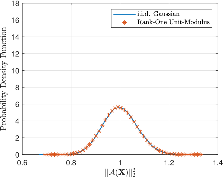
(a) $K=200$

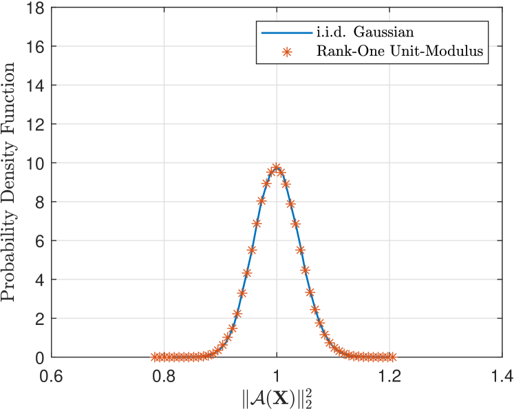
(b) $K=600$

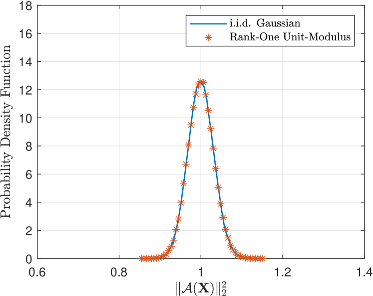
(c) $K=1000$

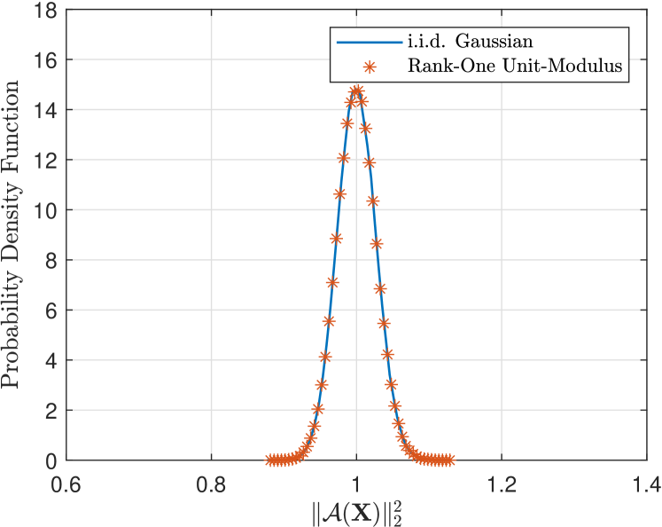
(d) $K=1400$

Fig. 1: Probability Density Function of $\|{\mathcal{A}}(\mathbf{X})\|_{2}^{2}$ with Different Number of Measurements

5 Numerical Experiments

In this section, we verify that the linear map generated by the random unit-modulus satisfies the RIP. Subsequently, we assess the recovery performance of low-rank matrices by employing this linear map.

Directly validating the RIP of the linear map is known to be NP-hard. Hence, we opt to demonstrate that the sufficient condition for RIP as outlined in Theorem 1 holds true. This condition suggests that the value of $\|\mathcal{A}(\mathbf{X})\|_{F}^{2}$ associated with unit-modulus vectors is highly concentrated around its expected value, which is $\|\mathbf{X}\|_{F}^{2}$. To illustrate this, we conduct an experiment as presented in Fig. 1. In this experiment, we randomly generate a fixed $\mathbf{X}\in\mathbb{C}^{40\times 80}$ with $\|\mathbf{X}\|_{F}=1$ and examine the probability density functions of $\|\mathcal{A}(\mathbf{X})\|_{F}^{2}$ by using two types of linear map. The first is generated by the rank-one model using random unit-modulus vectors, while the second serves as the benchmark and is based on i.i.d. Gaussian $\mathbf{A}_{k}$.

As depicted in Fig. 1, it is evident that the value of $\|{\mathcal{A}}(\mathbf{X})\|_{F}^{2}$ generated by rank-one measurements with random unit-modulus vectors is concentrated around its expectation $\|\mathbf{X}\|_{F}^{2}$ for different number of measurements. Comparing this outcome to the scenario where the entries of measurement matrix $\mathbf{A}_{k}$ are i.i.d. Gaussian, we observe that the probability density function gap between these two scenarios is notably narrow. Therefore, according to Theorem 1, the linear map employing the random rank-one unit-modulus measurements satisfies the RIP with high probability, similar to the scenario using i.i.d. Gaussian $\mathbf{A}_{k}$. Furthermore, as the number of measurements $K$ increases, both the Gaussian and rank-one unit-modulus curves become increasingly tightly concentrated around the expected value $\|\mathbf{X}\|_{F}^{2}$. This is consistent with the results in Theorem 5, where the tail bound exponentially decreases with the number of measurements $K$.

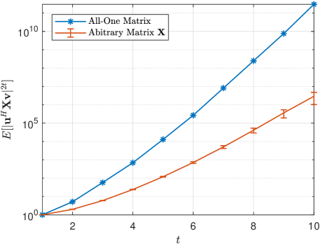
Fig. 2: Comparison of Two Expectations: All-One Matrix Scenario $\frac{1}{M^{t}N^{t}}{\mathbb{E}}[|\mathbf{u}^{H}\bm{1}\bm{1}^{T}\mathbf{v}|^{2t}]$ and Arbitrary Matrix Scenario ${\mathbb{E}}[|\mathbf{u}^{H}\mathbf{X}\mathbf{v}|^{2t}]$

Since the results in Theorem 4 are essential in the derivation of RIP analysis, we conduct an experiment in Fig. 2 to confirm the correctness of Theorem 4. Specifically, in Theorem 4, we have established the fact: under the constraint $\|\mathbf{X}\|_{F}=1$, the random variable $|\mathbf{u}^{H}\mathbf{X}\mathbf{v}|$ achieves the largest $(2t)^{th}$ moment when $\mathbf{X}=\frac{1}{\sqrt{MN}}\mathbf{1}\mathbf{1}^{T}$. In other words, we conclude that $\mathbb{E}[|\mathbf{u}^{H}\mathbf{X}\mathbf{v}|^{2t}]\leq\frac{1}{M^{t}N^{t}}\mathbb{E}[|\mathbf{u}^{H}\mathbf{1}\mathbf{1}^{T}\mathbf{v}|^{2t}],\forall\,t$. For the experiment in Fig. 2, we randomly generate $100$ matrices $\mathbf{X}\in\mathbb{C}^{40\times 80}$ and empirically calculate $\mathbb{E}[|\mathbf{u}^{H}\mathbf{X}\mathbf{v}|^{2t}]$ for each $\mathbf{X}$ and $t=1,2,\ldots,10$. The blue line represents the scenario of the all-one matrix, $\frac{1}{M^{t}N^{t}}\mathbb{E}[|\mathbf{u}^{H}\mathbf{1}\mathbf{1}^{T}\mathbf{v}|^{2t}]$. The red curve illustrates the mean and standard deviation for the $100$ realizations of arbitrary $\mathbf{X}$. Upon reviewing Fig. 2, we can readily observe that $\mathbb{E}[|\mathbf{u}^{H}\mathbf{X}\mathbf{v}|^{2t}]\leq{1}/{(M^{t}N^{t})}\mathbb{E}[|\mathbf{u}^{H}\mathbf{1}\mathbf{1}^{T}\mathbf{v}|^{2t}],\forall\,t$. Therefore, the value of $\mathbb{E}[|\mathbf{u}^{H}\mathbf{X}\mathbf{v}|^{2t}]$ is maximized when the matrix $\mathbf{X}$ has the form of the all-one matrix, i.e., $\mathbf{X}=\frac{1}{\sqrt{MN}}\mathbf{1}\mathbf{1}^{T}$. In conclusion, these experimental results are in perfect alignment with our analysis in Theorem 4.

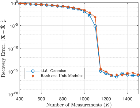
Fig. 3: Recovery Error of Low-Rank Matrix by Using Rank-One Unit-Modulus and i.i.d. Gaussian Measurements with Different Number of Measurements

In Fig. 3, we evaluate the low-rank matrix recovery performance by using the linear map of the rank-one unit-modulus measurements and i.i.d. measurement matrix $\mathbf{A}_{k}$. We randomly generate the target complex low-rank matrix $\mathbf{X}$ with dimension of $40\times 80$ of rank $r=5$. We let the number of measurements $K$ vary from $400$ to $1500$. For fair comparison, we utilize the well-known nuclear norm minimization (Recht et al., 2010) to recover the low-rank matrix from the measurements. The optimization problem is given by

$$\begin{split}&\min_{\mathbf{X}}\|\mathbf{X}\|_{*}\\ &\text{subject to }{\mathcal{A}}(\mathbf{X})=\mathbf{y}.\end{split}$$

We can refer to the findings in (Recht et al., 2010) that the recovery error by using i.i.d. $\mathbf{A}_{k}$ decreases with the number of measurements $K$. As evident in Fig. 3, the recovery error of the designed linear map exhibits a similar trend as the case of i.i.d. Gaussian. Moreover, observe that there is a sharp transition to near zero error at around $1100$ measurements for these two scenarios, which is consistent with the results in (Recht et al., 2010). Overall, the observations in Fig. 3 suggest that rank-one measurements with unit-modulus vectors achieves a recovery performance similar to that of i.i.d. Gaussian $\mathbf{A}_{k}$. Additional numiercal experiments about the recovery performance by using non-convex matrix recovery algorithms are attached in Section C of the supplementary materials.

Furthermore, the use of unit-modulus vectors allows for more efficient memory storage for the linear map, reducing the hardware costs associated with the linear map. As we have analyzed, this type of linear map not only satisfies the RIP but also exhibits similar recovery performance as the case of i.i.d. measurement matrices, as demonstrated in our experiments. Therefore, these advantages position our designed rank-one measurements with unit-modulus vectors as a promising linear map in low-rank matrix recovery.

6 Conclusion

In this paper, we have conducted a comprehensive RIP analysis for rank-one measurements with random unit-modulus vectors. The symmetric statistical properties of unit-modulus vectors have allowed us to derive the tail bound which exponentially decrease with the number of measurements . In comparison to the scenario of i.i.d. measurement matrices, the linear map generated by unit-modulus vectors not only satisfies the RIP but also offers the high memory efficiency. These advantageous properties show the potential of rank-one unit-modulus measurements as a highly effective linear map in the field of low-rank matrix recovery.

The supplementary materials contain detailed proofs of the results that are missing in the main paper, and additional experiments are provided as well.

A Proof of Theorem 4

After standard manipulations, one can find that

$${\mathbb{E}}[|\mathbf{u}^{H}\mathbf{X}\mathbf{v}|^{2t}]\leq{\mathbb{E}}[|\mathbf{u}^{H}\bar{\mathbf{X}}\mathbf{v}|^{2t}],$$

where each entry in $\bar{\mathbf{X}}$ is equal to the absolute value of the corresponding entry in $\mathbf{X}$. Therefore, it remains to show that

$${\mathbb{E}}[|\mathbf{u}^{H}\bar{\mathbf{X}}\mathbf{v}|^{2t}]\leq\frac{1}{M^{t}N^{t}}{\mathbb{E}}[|\mathbf{u}^{H}\bm{1}\bm{1}^{T}\mathbf{v}|^{2t}].$$

For the easy notation, we let $\mathbf{X}=\bar{\mathbf{X}}$. Denoting $\mathbf{X}_{m,:}$ as the $m$th row of $\mathbf{X}$, we have

$${\mathbb{E}}\left[|\mathbf{u}^{H}\mathbf{X}\mathbf{v}|^{2t}\right]={\mathbb{E}}\left[\left(\sum_{m}u_{m}^{*}\mathbf{X}_{m,:}\mathbf{v}\right)^{t}\left(\sum_{m}u_{m}\mathbf{X}_{m,:}\mathbf{v}^{*}\right)^{t}\right].$$

Then, according to the multinomial theorem, we have

$${\mathbb{E}}\left[|\mathbf{u}^{H}\mathbf{X}\mathbf{v}|^{2t}\right]$$

$$={\mathbb{E}}\left[\sum_{k_{1}+\ldots+k_{M}=t}\binom{t}{k_{1},\ldots,k_{M}}\prod(u_{m}^{*}\mathbf{X}_{1,:}\mathbf{v})^{k_{m}}\sum_{k_{1}^{\prime}+\ldots+k_{M}^{\prime}=t}\binom{t}{k^{\prime}_{1},\ldots,k_{M}^{\prime}}\prod(u_{m}\mathbf{X}_{m,:}\mathbf{v}^{*})^{k^{\prime}_{m}}\right]$$

$$={\mathbb{E}}\left[\sum_{k_{1}+\ldots+k_{M}=t}{\binom{t}{k_{1},\ldots,k_{M}}}^{2}\prod|\mathbf{X}_{m,:}\mathbf{v}|^{2k_{m}}\right].$$ (23)

For the concise proof, we express $\mathbf{X}_{m,:}=c_{m}\mathbf{x}_{m}^{T}$ where $\|\mathbf{x}_{m}\|_{2}=1$. Without loss generality, we assume $c_{m}\geq 0,\forall\,m$. Then we rewrite the expression 23 above as

$${\mathbb{E}}\left[\sum_{k_{1}+\ldots+k_{M}=t}{\binom{t}{k_{1},\ldots,k_{M}}}^{2}\prod|\mathbf{X}_{m,:}\mathbf{v}|^{2k_{m}}\right]$$

$$={\mathbb{E}}\left[\sum_{k_{1}+\ldots+k_{M}=t}{\binom{t}{k_{1},\ldots,k_{M}}}^{2}\prod|\mathbf{x}_{m}^{T}\mathbf{v}|^{2k_{m}}\prod_{i=1}^{M}c_{m}^{2k_{m}}\right].$$

Then, according to Lemma 4, we have

$${\mathbb{E}}\left[\prod|\mathbf{x}_{m}^{T}\mathbf{v}|^{2k_{m}}\right]\leq\max_{m}{\mathbb{E}}\left[|\mathbf{x}_{m}^{T}\mathbf{v}|^{2t}\right].$$

Thus, the value of ${\mathbb{E}}\left[|\mathbf{u}^{H}\mathbf{X}\mathbf{v}|^{2t}\right]$ in 23 is upper bounded by

$${\mathbb{E}}\left[|\mathbf{u}^{H}\mathbf{X}\mathbf{v}|^{2t}\right] \leq\sum_{k_{1}+\ldots+k_{M}=t}{\binom{t}{k_{1},\ldots,k_{M}}}^{2}\max_{m}{\mathbb{E}}\left[|\mathbf{x}_{m}^{T}\mathbf{v}|^{2t}\right]\prod_{i=1}^{M}c_{m}^{2k_{m}}$$

$$={\mathbb{E}}\left[|\mathbf{u}^{H}\mathbf{X}^{*}\mathbf{v}|^{2t}\right],$$

where $\mathbf{X}^{*}=[c_{1}\mathbf{x}_{m^{*}},c_{2}\mathbf{x}_{m^{*}},\cdots,c_{M}\mathbf{x}_{m^{*}}]^{T}$ and $m^{*}=\operatorname*{arg\,max}_{m}{\mathbb{E}}\left[|\mathbf{X}_{m,:}\mathbf{v}|^{2t}\right]$. In other words,

$${\mathbb{E}}\left[|\mathbf{u}^{H}\mathbf{X}\mathbf{v}|^{2t}\right] \leq{\mathbb{E}}\left[|\mathbf{u}^{H}\mathbf{X}^{*}\mathbf{v}|^{2t}\right]$$

$$=\sum_{k_{1}+\ldots+k_{M}=t}{\binom{t}{k_{1},\ldots,k_{M}}}^{2}{\mathbb{E}}\left[|\mathbf{x}_{m^{*}}^{T}\mathbf{v}|^{2t}\right]\prod_{i=1}^{M}c_{m}^{2k_{m}}$$

$$=\underbrace{{\mathbb{E}}\left[|\mathbf{x}_{m^{*}}^{T}\mathbf{v}|^{2t}\right]}_{\text{first part}}\underbrace{\sum_{k_{1}+\ldots+k_{M}=t}{\binom{t}{k_{1},\ldots,k_{M}}}^{2}\prod_{i=1}^{M}c_{m}^{2k_{m}}}_{\text{second part}}.$$ (24)

By Theorem 3, the first part of value in 24 is maximized when the entries in $\mathbf{x}_{m^{*}}$ are equivalent. According to Lemma 2, the second part is maximized when $c_{m}=\sqrt{\frac{1}{M}}$. Recall that $\mathbf{X}^{*}=[c_{1}\mathbf{x}_{m^{*}},c_{2}\mathbf{x}_{m^{*}},\cdots,c_{M}\mathbf{x}_{m^{*}}]^{T}$, after substituting the setting of $\mathbf{x}_{m^{*}}$ and $c_{m}$ into the expression of $\mathbf{X}^{*}$, one can easily check the corresponding matrix is expressed as $\mathbf{X}^{*}=\frac{1}{\sqrt{MN}}\bm{1}\bm{1}^{T}$. Thus, we have

$${\mathbb{E}}\left[|\mathbf{u}^{H}\mathbf{X}\mathbf{v}|^{2t}\right]\leq\frac{1}{M^{t}N^{t}}{\mathbb{E}}[|\mathbf{u}^{H}\bm{1}\bm{1}^{T}\mathbf{v}|^{2t}].$$

This concludes the proof. ∎

B Proof of Preliminaries

B.1 Proof of Lemma 1

Note that the Legendre polynomials $P_{n}(x)$ is expressed as

$$P_{n}(x)=\frac{1}{2^{n}}\sum_{k=0}^{n}\binom{n}{k}^{2}(x-1)^{n-k}(x+1)^{k}.$$

After simple manipulations, the expression of $s_{n}(p)$ is expressed as

$$s_{n}(p)=(2p-1)^{n}P_{n}\left(\frac{1}{2p-1}\right).$$

After performing first-order derivative, one can check that the value of $s_{n}$ is maximized when $p=1/2$. ∎

B.2 Proof of Theorem 3

Without loss of generality, we can assume that entries in $\mathbf{x}$ are non-negative, i.e., $x_{n}\geq 0,\forall\,n$. This is because ${\mathbb{E}}\left[|\mathbf{x}^{T}\mathbf{v}|^{2m}\right]\leq{\mathbb{E}}\left[|\bar{\mathbf{x}}^{T}\mathbf{v}|^{2m}\right]$. Then, the expression of ${\mathbb{E}}\left[|\mathbf{x}^{T}\mathbf{v}|^{2_{m}}\right]$ is

$${\mathbb{E}}\left[|\mathbf{x}^{T}\mathbf{v}|^{2m}\right]={\mathbb{E}}\left[\left(x_{1}v_{1}+\ldots+x_{N}v_{N}\right)^{m}\left(x_{1}v_{1}^{*}+\ldots+x_{N}v_{N}^{*}\right)^{m}\right].$$ (25)

Without loss of generality, we assume $x_{1}\neq x_{2}$. To complete the proof, we will show that by letting $x_{1}=x_{2}=\sqrt{\frac{x_{1}^{2}+x_{2}^{2}}{2}}$, the expectation in 25 will increase. Here, we denote $y=\sum_{n=3}^{N}x_{n}v_{n}$, and $t=\sum_{n=3}^{N}x_{n}^{2}$. Therefore, we have $x_{1}^{2}+x_{2}^{2}=1-t$. Then, according to the multinomial theorem, we have

$${\mathbb{E}}\left[|\mathbf{x}^{T}\mathbf{v}|^{2_{m}}\right] ={\mathbb{E}}\left[\left(x_{1}v_{1}+x_{2}v_{2}+y\right)^{m}\left(x_{1}v_{1}^{*}+x_{2}v_{2}^{*}+y^{*}\right)^{m}\right]$$

$$={\mathbb{E}}\Biggl{[}\sum_{k_{1}+k_{2}+k_{3}=m}\binom{m}{k_{1},k_{2},k_{3}}(x_{1}v_{1})^{k_{1}}(x_{2}v_{2})^{k_{2}}y^{k_{3}}$$

$$~{}~{}~{}~{}~{}~{}~{}~{}\sum_{k_{1}^{\prime}+k_{2}^{\prime}+k_{3}^{\prime}=m}\binom{m}{k_{1}^{\prime},k_{2}^{\prime},k_{3}^{\prime}}(x_{1}v_{1}^{*})^{k_{1}^{\prime}}(x_{2}v_{2}^{*})^{k_{2}^{\prime}}y^{k_{3}^{\prime}}\Biggr{]}.$$

Because of the property of expectation, the expression above can be written in

$$\sum_{k_{1}+k_{2}+k_{3}=m}{\binom{m}{k_{1},k_{2},k_{3}}}^{2}(x_{1})^{2k_{1}}(x_{2})^{2k_{2}}{\mathbb{E}}\left[|y|^{2k_{3}}\right]$$

$$=\sum_{k_{3}=0}^{m}\sum_{k_{1}+k_{2}=m-k_{3}}{\binom{m}{k_{1},k_{2},k_{3}}}^{2}(x_{1})^{2k_{1}}(x_{2})^{2k_{2}}{\mathbb{E}}\left[|y|^{2k_{3}}\right]$$

$$=\sum_{k_{3}=0}^{m}\sum_{k_{1}+k_{2}=m-k_{3}}{\binom{m}{k_{3},m-k_{3}}}^{2}{\binom{m-k_{3}}{k_{1},k_{2}}}^{2}(x_{1})^{2k_{1}}(x_{2})^{2k_{2}}{\mathbb{E}}\left[|y|^{2k_{3}}\right]$$

$$=\sum_{k_{3}=0}^{m}{\binom{m}{k_{3},m-k_{3}}}^{2}{\mathbb{E}}\left[|y|^{2k_{3}}\right]\sum_{k_{1}+k_{2}=m-k_{3}}{\binom{m-k_{3}}{k_{1},k_{2}}}^{2}(x_{1})^{2k_{1}}(x_{2})^{2k_{2}}.$$

Based on Corollary 1, the value of $\sum_{k_{1}+k_{2}=m-k_{3}}{\binom{m-k_{3}}{k_{1},k_{2}}}^{2}(x_{1})^{2k_{1}}(x_{2})^{2k_{2}}$ is maximized when $x_{1}^{2}=x_{2}^{2}=\frac{1-t}{2}$. Because we assume the positiveness, we will have that $x_{1}=x_{2}=\sqrt{\frac{1-t}{2}}$. This concludes the proof. ∎

B.3 Proof of Lemma 2

Without loss of generality, we assume $c_{1}\neq c_{2}$ while $c_{1}^{2}+c_{2}^{2}$ is a constant. Similar to the proof in Section B.2, it is sufficient to prove that making $c_{1}=c_{2}$ can increase the value in 12. Then, the general result in Lemma 2 can be obtained by induction. First of all, separating $c_{1},c_{2}$ with $c_{m},\forall\,m\geq 3$ gives the following,

$$\sum_{k_{1}+\ldots+k_{M}=t}{\binom{t}{k_{1},\ldots,k_{M}}}^{2}\prod_{m=1}^{M}c_{m}^{2k_{m}}$$

$$=\sum_{k_{1}+\ldots+k_{M}=t}{\binom{t}{k_{1},\ldots,k_{M}}}^{2}c_{1}^{2k_{1}}c_{2}^{2k_{2}}\prod_{m=3}^{M}c_{m}^{2k_{m}}$$

$$=\sum_{t_{0}=0}^{t}\sum_{k_{1}+k_{2}=t_{0}}\sum_{k_{3}+,\ldots,k_{M}=t-t_{0}}{\binom{t}{k_{1},\ldots,k_{M}}}^{2}c_{1}^{2k_{1}}c_{2}^{2k_{2}}\prod_{m=3}^{M}c_{m}^{2k_{m}}$$

$$=\sum_{t_{0}=0}^{t}\sum_{k_{1}+k_{2}=t_{0}}\sum_{k_{3}+,\ldots,k_{M}=t-t_{0}}{\binom{t}{t_{0},t-t_{0}}}^{2}{\binom{t_{0}}{k_{1},k_{2}}}^{2}{\binom{t-t_{0}}{k_{3},\ldots,k_{m}}}^{2}c_{1}^{2k_{1}}c_{2}^{2k_{2}}\prod_{m=3}^{M}c_{m}^{2k_{m}}.$$

Then, according to Corollary 1, we have the following inquality,

$$\sum_{k_{1}+k_{2}=t_{0}}{\binom{t_{0}}{k_{1},k_{2}}}^{2}c_{1}^{2k_{1}}c_{2}^{2k_{2}}\leq\sum_{k_{1}+k_{2}=t_{0}}{\binom{t_{0}}{k_{1},k_{2}}}^{2}\left(\frac{c_{1}^{2}+c_{2}^{2}}{2}\right)^{t_{0}},$$

where the equality holds when $c_{1}=c_{2}=\sqrt{\frac{c_{1}^{2}+c_{2}^{2}}{2}}$. This concludes the proof.

B.4 Proof of Lemma 3

We mainly use the Hölder’s inequality for the proof of Lemma 3. Specifically, for positive random variables $X$ and $Y$, if $1/p+1/q=1$, then Hölder’s inequality shows that

$${\mathbb{E}}[XY]\leq({\mathbb{E}}[X^{p}])^{1/p}({\mathbb{E}}[Y^{q}])^{1/q}.$$

For the posted problem, we let $X=X_{1}^{k_{1}}$ and $Y=X_{2}^{k_{2}}$, then we have

$${\mathbb{E}}[X_{1}^{k_{1}}X_{2}^{k_{2}}]\leq({\mathbb{E}}[X_{1}^{k_{1}p}])^{1/p}({\mathbb{E}}[X_{2}^{k_{2}q}])^{1/q}.$$

which concludes the proof of 13.

When $k_{1}=0$ or $k_{2}=0$, the inequality in 14 holds trivially. Here, without loss of generality, we assume $k_{1},k_{2}\neq 0$. By letting $p=\frac{k_{1}+k_{2}}{k_{1}}$ and $q=\frac{k_{1}+k_{2}}{k_{2}}$ in the expression 13, one can check that $1/p+1/q=1$. Then, the following inequality holds due to the Hölder’s inequality,

$${\mathbb{E}}[X_{1}^{k_{1}}X_{2}^{k_{2}}] \leq({\mathbb{E}}[X_{1}^{k_{1}+k_{2}}])^{\frac{k_{1}}{k_{1}+k_{2}}}({\mathbb{E}}[X_{2}^{k_{1}+k_{2}}])^{\frac{k_{2}}{k_{1}+k_{2}}}$$

$$\leq\max\{{\mathbb{E}}[X_{1}^{k_{1}+k_{2}}],{\mathbb{E}}[X_{2}^{k_{1}+k_{2}}]\}.$$

Thus, this concludes the proof of the result in 14. ∎

B.5 Proof of Lemma 4

Without loss of generality, we assume $k_{n}>0,\forall\,n$. Using the Hölder’s inequality, we have

$${\mathbb{E}}\left[X_{1}^{k_{1}}\cdots X_{N-1}^{k_{N-1}}X_{N}^{k_{N}}\right]\leq\left({\mathbb{E}}\left[\left(X_{1}^{k_{1}}\cdots X_{N-1}^{k_{N-1}}\right)^{\frac{t}{t-k_{N}}}~{}\right]\right)^{\frac{t-k_{N}}{t}}\left({\mathbb{E}}\left[(X_{N}^{k_{N}})^{t/k_{N}}\right]\right)^{k_{N}/t},$$ (26)

where $p=t/(t-k_{N})$ and $q=t/k_{N}$. Simplifying the R.H.S. in 26 yields

$${\mathbb{E}}\left[X_{1}^{k_{1}}\cdots X_{N-1}^{k_{N-1}}X_{N}^{k_{N}}\right]\leq\left({\mathbb{E}}\left[\left(X_{1}^{k_{1}}\cdots X_{N-1}^{k_{N-1}}\right)^{t/(t-k_{N})}~{}\right]\right)^{(t-k_{N})/t}\left({\mathbb{E}}\left[X_{N}^{t}\right]\right)^{k_{N}/t}.$$ (27)

Again, using Hölder’s inequality for the first part of R.H.S. of 27 with $p=\frac{t-k_{N}}{t-k_{N}-k_{N-1}}$ and $q={\frac{t-k_{N}}{k_{N-1}}}$, we have

$${\mathbb{E}}\left[\left(X_{1}^{k_{1}}\cdots X_{N-1}^{k_{N-1}}\right)^{t/(t-k_{N})}\right]$$

$$={\mathbb{E}}\left[\left(X_{1}^{k_{1}}\cdots X_{N-2}^{k_{N-2}}\right)^{t/(t-k_{N})}X_{N-1}^{k_{N-1}\frac{t}{t-k_{N}}}\right]$$

$$\leq\left({\mathbb{E}}\left[\left(X_{1}^{k_{1}}\cdots X_{N-2}^{k_{N-2}}\right)^{\frac{t}{t-k_{N}}\frac{t-k_{N}}{t-k_{N}-k_{N-1}}}\right]\right)^{\frac{t-k_{N}-k_{N-1}}{t-k_{N}}}\left({\mathbb{E}}\left[\left(X_{N-1}^{k_{N-1}\frac{t}{t-k_{N}}}\right)^{\frac{t-k_{N}}{k_{N-1}}}\right]\right)^{\frac{k_{N-1}}{t-k_{N}}}$$

$$=\left({\mathbb{E}}\left[\left(X_{1}^{k_{1}}\cdots X_{N-2}^{k_{N-2}}\right)^{\frac{t}{t-k_{N}-k_{N-1}}}\right]\right)^{\frac{t-k_{N}-k_{N-1}}{t-k_{N}}}\left({\mathbb{E}}\left[X_{N-1}^{t}\right]\right)^{\frac{k_{N-1}}{t-k_{N}}}.$$

Substituting the above equation into 27 gives

$${\mathbb{E}}\left[X_{1}^{k_{1}}\cdots X_{N-1}^{k_{N-1}}X_{N}^{k_{N}}\right]$$

$$\leq\underbrace{\left({\mathbb{E}}\left[\left(X_{1}^{k_{1}}\cdots X_{N-2}^{k_{N-2}}\right)^{\frac{t}{t-k_{N}-k_{N-1}}}\right]\right)^{\frac{t-k_{N}-k_{N-1}}{t-k_{N}}}}_{\text{first part}}\underbrace{\left({\mathbb{E}}\left[X_{N-1}^{t}\right]\right)^{\frac{k_{N-1}}{t}}\left({\mathbb{E}}\left[X_{N}^{t}\right]\right)^{\frac{k_{N}}{t}}}_{\text{remaining parts}}.$$ (28)

For the first part in 28, we iteratively utilize the Hölder’s inequality, and finally obtain the following,

$${\mathbb{E}}\left[\prod_{n=1}^{N}X_{n}^{k_{n}}\right] \leq\prod_{n=1}^{N}\left({\mathbb{E}}\left[X_{n}^{t}\right]\right)^{k_{n}/t}$$

$$\leq\max_{n}{\mathbb{E}}\left[X_{n}^{t}\right].$$

This concludes the proof of Lemma 4. ∎

C ADDITIONAL EXPERIMENTS

In this section, we evaluate the recovery performance of non-convex low-rank matrix recovery algorithms by using the rank-one unit-modulus measurements and i.i.d. Gaussian measurements. Similar to the settings in Fig. 3, we randomly generate the target low-rank matrix $\mathbf{X}\in{\mathbb{C}}^{40\times 80}$ with a rank of $r=5$, and the number of measurements $K$ ranges from $500$ to $1500$. There are two typical non-convex algorithms considered in the experiments. Specifically, in Fig. 4 , we utilize the alternating minimization method (Jain et al., 2013) to recover the low-rank matrix from the rank-one unit-modulus measurements or the i.i.d. Gaussian measurements. In Fig. 5, we employ the gradient-based method (Chi et al., 2019) for matrix recovery task.

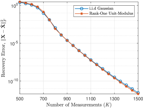
Fig. 4: Recovery Error of Alternating Minimization Method by Using Rank-One Unit-Modulus and i.i.d. Gaussian Measurements with Different Number of Measurements

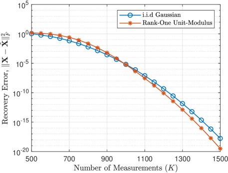
Fig. 5: Recovery Error of Gradient-Based Method by Using Rank-One Unit-Modulus and i.i.d. Gaussian Measurements with Different Number of Measurements

As we can see in Figs. 4 and 5, for both typical non-convex methods, i.e., alternating minimization method and gradient-based method, the designed rank-one measurements with random unit-modulus vectors achieves a recovery performance similar to that of i.i.d. Gaussian measurements. Therefore, by integrating the results of experiment in Fig. 3, regardless of whether convex or non-convex optimization algorithms are utilized, the rank-one unit-modulus measurements always exhibit a similar matrix recovery performance to that of i.i.d. measurements, which is attributed to the proven RIP results.

References

- Cai and Zhang (2015) T Tony Cai and Anru Zhang. ROP: Matrix recovery via rank-one projections. The Annals of Statistics, 43(1):102–138, 2015.
- Candes and Plan (2011) Emmanuel J Candes and Yaniv Plan. Tight oracle inequalities for low-rank matrix recovery from a minimal number of noisy random measurements. IEEE Transactions on Information Theory, 57(4):2342–2359, 2011.
- Candès and Recht (2009) Emmanuel J Candès and Benjamin Recht. Exact matrix completion via convex optimization. Foundations of Computational mathematics, 9(6):717–772, 2009.
- Candès and Tao (2010) Emmanuel J Candès and Terence Tao. The power of convex relaxation: Near-optimal matrix completion. IEEE Transactions on Information Theory, 56(5):2053–2080, 2010.
- Candes et al. (2013) Emmanuel J Candes, Thomas Strohmer, and Vladislav Voroninski. Phaselift: Exact and stable signal recovery from magnitude measurements via convex programming. Communications on Pure and Applied Mathematics, 66(8):1241–1274, 2013.
- Candes et al. (2015) Emmanuel J Candes, Xiaodong Li, and Mahdi Soltanolkotabi. Phase retrieval via wirtinger flow: Theory and algorithms. IEEE Transactions on Information Theory, 61(4):1985–2007, 2015.
- Chen and Chi (2018) Yudong Chen and Yuejie Chi. Harnessing structures in big data via guaranteed low-rank matrix estimation: Recent theory and fast algorithms via convex and nonconvex optimization. IEEE Signal Processing Magazine, 35(4):14–31, 2018.
- Chen et al. (2015) Yuxin Chen, Yuejie Chi, and Andrea J Goldsmith. Exact and stable covariance estimation from quadratic sampling via convex programming. IEEE Transactions on Information Theory, 61(7):4034–4059, 2015.
- Chi et al. (2019) Yuejie Chi, Yue M Lu, and Yuxin Chen. Nonconvex optimization meets low-rank matrix factorization: An overview. IEEE Transactions on Signal Processing, 67(20):5239–5269, 2019.
- Davenport and Romberg (2016) Mark A Davenport and Justin Romberg. An overview of low-rank matrix recovery from incomplete observations. IEEE Journal of Selected Topics in Signal Processing, 10(4):608–622, 2016.
- El Ayach et al. (2014) Omar El Ayach, Sridhar Rajagopal, Shadi Abu-Surra, Zhouyue Pi, and Robert W Heath. Spatially sparse precoding in millimeter wave mimo systems. IEEE Transactions on Wireless Communications, 13(3):1499–1513, 2014.
- Farias et al. (2022) Vivek Farias, Andrew A. Li, and Tianyi Peng. Uncertainty quantification for low-rank matrix completion with heterogeneous and sub-exponential noise. In Proceedings of the 25th International Conference on Artificial Intelligence and Statistics, pages 1179–1189. PMLR, 28–30 Mar 2022.
- Ge et al. (2017) Rong Ge, Chi Jin, and Yi Zheng. No spurious local minima in nonconvex low rank problems: A unified geometric analysis. In Proceedings of the 34th International Conference on Machine Learning, pages 1233–1242. PMLR, 2017.
- Jain et al. (2010) Prateek Jain, Raghu Meka, and Inderjit Dhillon. Guaranteed rank minimization via singular value projection. Advances in Neural Information Processing Systems, 23, 2010.
- Jain et al. (2013) Prateek Jain, Praneeth Netrapalli, and Sujay Sanghavi. Low-rank matrix completion using alternating minimization. In Proceedings of the 45th Annual ACM Symposium on Theory of Computing, pages 665–674, 2013.
- Kueng et al. (2017) Richard Kueng, Holger Rauhut, and Ulrich Terstiege. Low rank matrix recovery from rank one measurements. Applied and Computational Harmonic Analysis, 42(1):88–116, 2017.
- Li et al. (2019) Yuanxin Li, Cong Ma, Yuxin Chen, and Yuejie Chi. Nonconvex matrix factorization from rank-one measurements. In Proceedings of the 22nd International Conference on Artificial Intelligence and Statistics, pages 1496–1505. PMLR, 2019.
- Ma et al. (2018) Cong Ma, Kaizheng Wang, Yuejie Chi, and Yuxin Chen. Implicit regularization in nonconvex statistical estimation: Gradient descent converges linearly for phase retrieval and matrix completion. In Proceedings of the 35th International Conference on Machine Learning, pages 3345–3354. PMLR, 2018.
- Recht et al. (2010) Benjamin Recht, Maryam Fazel, and Pablo A Parrilo. Guaranteed minimum-rank solutions of linear matrix equations via nuclear norm minimization. SIAM review, 52(3):471–501, 2010.
- Richmond and Shallit (2008) Lawrence Bruce Richmond and Jeffrey Shallit. Counting abelian squares. arXiv preprint arXiv:0807.5028, 2008.
- Shechtman et al. (2015) Yoav Shechtman, Yonina C Eldar, Oren Cohen, Henry Nicholas Chapman, Jianwei Miao, and Mordechai Segev. Phase retrieval with application to optical imaging: a contemporary overview. IEEE signal processing magazine, 32(3):87–109, 2015.
- Tong et al. (2022) Tian Tong, Cong Ma, Ashley Prater-Bennette, Erin Tripp, and Yuejie Chi. Scaling and scalability: Provable nonconvex low-rank tensor completion. In Proceedings of the 25th International Conference on Artificial Intelligence and Statistics, pages 2607–2617. PMLR, 28–30 Mar 2022.
- Tu et al. (2016) Stephen Tu, Ross Boczar, Max Simchowitz, Mahdi Soltanolkotabi, and Ben Recht. Low-rank solutions of linear matrix equations via procrustes flow. In Proceedings of the 33rd International Conference on Machine Learning, pages 964–973. PMLR, 2016.
- Zhang et al. (2018a) Richard Zhang, Cédric Josz, Somayeh Sojoudi, and Javad Lavaei. How much restricted isometry is needed in nonconvex matrix recovery? Advances in Neural Information Processing Systems, 31, 2018a.
- Zhang and Tay (2021) Wei Zhang and Wee Peng Tay. Cost-efficient RIS-aided channel estimation via rank-one matrix factorization. IEEE Wireless Communications Letters, 10(11):2562–2566, 2021.
- Zhang et al. (2018b) Wei Zhang, Taejoon Kim, David J Love, and Erik Perrins. Leveraging the restricted isometry property: Improved low-rank subspace decomposition for hybrid millimeter-wave systems. IEEE Transactions on Communications, 66(11):5814–5827, 2018b.
- Zhang et al. (2019) Wei Zhang, Taejoon Kim, Guojun Xiong, and Shu-Hung Leung. Leveraging subspace information for low-rank matrix reconstruction. Signal Processing, 163:123–131, 2019. ISSN 0165-1684.
- Zhang et al. (2020) Wei Zhang, Taejoon Kim, and Shu-Hung Leung. A sequential subspace method for millimeter wave MIMO channel estimation. IEEE Transactions on Vehicular Technology, 69(5):5355–5368, 2020.
- Zheng and Lafferty (2015) Qinqing Zheng and John Lafferty. A convergent gradient descent algorithm for rank minimization and semidefinite programming from random linear measurements. Advances in Neural Information Processing Systems, 28, 2015.