Few-shot Learner Parameterization by Diffusion Time-steps
Abstract
Even when using large multi-modal foundation models, few-shot learning is still challenging—if there is no proper inductive bias, it is nearly impossible to keep the nuanced class attributes while removing the visually prominent attributes that spuriously correlate with class labels. To this end, we find an inductive bias that the time-steps of a Diffusion Model (DM) can isolate the nuanced class attributes, i.e., as the forward diffusion adds noise to an image at each time-step, nuanced attributes are usually lost at an earlier time-step than the spurious attributes that are visually prominent. Building on this, we propose Time-step Few-shot (TiF) learner. We train class-specific low-rank adapters for a text-conditioned DM to make up for the lost attributes, such that images can be accurately reconstructed from their noisy ones given a prompt. Hence, at a small time-step, the adapter and prompt are essentially a parameterization of only the nuanced class attributes. For a test image, we can use the parameterization to only extract the nuanced class attributes for classification. TiF learner significantly outperforms OpenCLIP and its adapters on a variety of fine-grained and customized few-shot learning tasks. Codes are in https://github.com/yue-zhongqi/tif .
1 Introduction
Multi-modal foundation models, e.g., CLIP [26], have recently demonstrated remarkable zero-shot performance in general visual classification tasks [3, 25]. They define a task by a suitable text prompt for each class (e.g., “a photo of an aircraft” for the class “aircraft”), and use the model to classify an image by selecting the class prompt with the highest “image-prompt” similarity. However, the zero-shot paradigm encounters limitations when one cannot find a proper prompt to accurately describe the class of interest. This is particularly true for niche and fine-grained categories whose names may not encapsulate the subtle visual features recognizable by the model (e.g., “707-320 aircraft”), or for customized categories where it is impractical to fully describe their specification through text alone (e.g., a specific person). For these situations, a few-shot training set is necessary to define the classification on demand.

The most common approach is to train an auxiliary feature adapter attached after the CLIP visual encoder [8, 44] or text encoder [48, 47]. The objective is to align the adapted image feature with its prompt embedding only from the same class. However, it is well-known that such discriminative training on few-shot examples is biased to spurious correlations [41], which hinders generalization at test time. For example, in Figure 1, consider a scenario where aircraft A and B is defined by a subtle class attribute, e.g., window, but a visually prominent attribute happens to spuriously correlate with the class labels in the few-shot training set, i.e., A appearing with background sky and B with ground. The model will erroneously consider both window and background attributes for inaccurate prediction, e.g., predicting B with sky as A. Frustratingly, it is impossible to isolate the nuanced class attributes from visually prominent yet spurious ones without an explicit inductive bias (e.g., prior knowledge that “windows” is a class attribute) [5, 21].
To address the challenge, we turn our attention to generative classifiers [24], inspired by the recent advancement in the text-conditioned generative Diffusion Model (DM) [28]. DM has enabled extrapolation to novel attribute combinations by textual control (e.g., generating “Salvador Dalí with a robotic half-face”). Hence ideally, one could prompt DM with all attribute combinations for each class (e.g., “B with sky” and “B with ground”) to synthesize a diverse training set, where no attribute is biased. Unfortunately, this approach is impractical yet, since there is no ground-truth of a complete attribute inventory.
In this paper, we introduce a practical solution by revealing that nuanced class attributes and visually prominent ones are naturally isolated by diffusion time-steps, lending itself to de-biasing. Specifically, DM defines a forward process that gradually injects Gaussian noise into each image over time-steps, creating a sequence of noisy images that progressively collapse to pure noise. As increases, we show in Figure 2 (top) that more visual attributes are lost when they become indistinguishable. Notably, we prove in Section 3.3 that nuanced class attributes (e.g., windows defining class A, B) are lost at an early time-step, while visually prominent ones (e.g., the spurious background) are lost later. This motivates our approach:
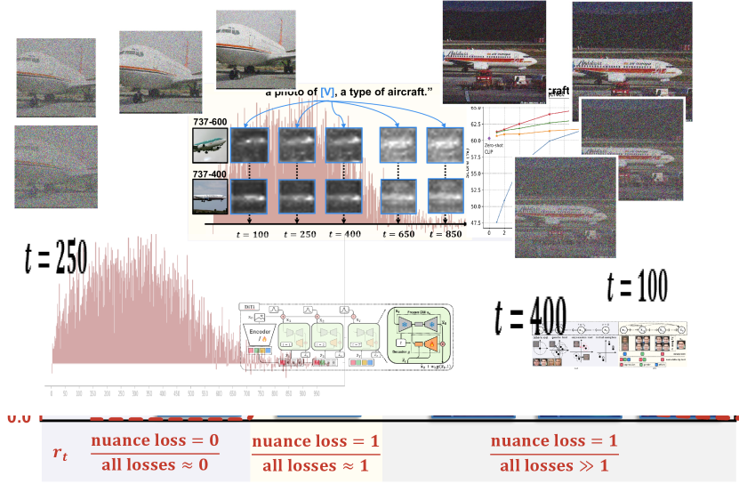
(\@slowromancapi@) Parameterization. For each class , we train a denoising network parameterized by to reconstruct each image in its training set from the noisy and a text prompt (details given below), i.e., by minimizing the reconstruction error for all . When training converges with accurate reconstruction, must make up for the lost attributes in each using . Hence is essentially a parameterization of the lost attributes at for class . Particularly, we adopt a low-rank implementation of , such that at a small is constrained to parameterize only the lost nuances of , without accidentally capturing the visually prominent attributes that are not lost yet. We visualize this in Figure 2 bottom by attention map, e.g., indeed parameterizes the visual attribute about window at when it becomes lost.
(\@slowromancapii@) De-biasing by Time-steps. We classify a test image by selecting with the least reconstruction error at a small time-step . This inference rule is not affected by the spurious correlations, because from the analysis above, such parameterize only the nuanced attributes that define ’s class, free from the visually prominent ones that are spurious.
We term our approach as the Time-step Few-shot (TiF) learner. We implement the above two points as below:
(\@slowromancapi@) We inject Low-Rank Adaptation (LoRA) matrices [13] into a pre-trained, frozen DM and denote their parameters as . We follow DreamBooth [30] to use a rare token identifier [V] (e.g., “hta”) to form the prompt , such that it can be easily re-associated to the specificity of each class.
(\@slowromancapii@) To avoid searching for the best “small ”, we design a hyper-parameter-free approach. We first derive an equation that measures the degree of attribute loss in Section 3.3. Then we compute a ratio of nuanced attribute loss over all attribute losses at each to calculate a weighted reconstruction error for inference. As shown in Figure 2 red line, the weight reaches its peak when nuances become lost at a small , and diminishes to 0 when more attributes become lost as increases. Hence the weighted error accounts only for the inability of each in making up the nuanced class attribute to de-bias.
The contribution of the paper is summarized below.
- •
-
•
Motivated by our theoretical insights, we present a straightforward yet effective FSL approach that mitigates spurious correlations (Section 4).
-
•
On fine-grained classification, Re-Identification and medical image classification, TiF learner significantly outperforms the powerful OpenCLIP and its adapters in various few-shot settings by up to 21.6%.
2 Related Works
Conventional FSL typically adopts a pre-training, meta-learning and fine-tuning paradigm [2, 43]. The first stage aims to capture rich prior knowledge as a feature backbone [6]. The second stage trains the model on “sandbox” FSL tasks to tailor it for the target task, e.g., learning a classifier weight generator [9], a distance kernel function in -NN [39], a feature space to better seprate the classes [39, 43], or even an initialization of the classifier [7]. The final stage involves training a classifier on the few-shot examples. However, multi-modal foundation models already capture extremely profound prior knowledge, hence recent works focus on few-shot adapting such models.
FSL with Foundation Models. There are two main approaches that both leverage CLIP. First is prompt tuning, which aims to learn a prompt for each class. CoOp [48] learns a continuous prompt embedding instead of using a hand-crafted prompt. CoCoOp [47] extends CoOp by learning an image conditional prompt. ProGrad [49] aligns the prompt gradient to the general knowledge of CLIP. Recent MaPLe [15] additionally fine-tune the CLIP visual encoder. The other line aims to learn a CLIP visual feature adapter. CLIP-Adapter [8] applies a lightweight residual-style adapter, followed by the training-free approach Tip-Adapter [44]. CALIP [10] proposes a parameter-free attention to improve both zero-shot and few-shot performance. The recent CaFo [45] ensembles multiple foundation models to help with feature adaptation. However, they still suffer from the spurious correlation. Besides CLIP-based approaches, recent works have explored in-context learning with vision-language models [1], yet their current classification accuracy still lags behind.
3 Problem Formulations
3.1 Few-Shot Learning
We aim to solve a -way--shot Few-Shot Learning (FSL) task: train a model to classify categories using the few-shot dataset , where each category has a small number of images. In particular, we use the notation in causal representation learning [11, 32]: each image from is generated by , where is the generator, denotes the class attribute that define the category (e.g., “many windows” for class “707-320”), and denotes other environmental attribute (e.g., “sky background”). Note that is a category index, and denotes its defining attribute. Hence the crux of FSL is to pinpoint for classification and discard the irrelevant .
Necessity of FSL. The zero-shot accuracy of multi-modal foundation models matches that of a fully-supervised model on common visual categories [3, 25] (e.g., ImageNet [31]), rendering FSL unnecessary on those tasks. Specifically, such model takes an image and a text prompt that describes as input, and outputs the similarity between and . For example, , where is the cosine similarity, denotes the CLIP visual and text encoder, respectively. Therefore we can predict an image in a zero-shot setting as follows
| (1) |
Hence we focus on scenarios where the zero-shot paradigm is limited—when is about nuanced details on fine-grained or customized categories, it is impractical to find a prompt recognizable by the model that encapsulates the intricacies of , thereby requiring a few-shot set to define .
Challenge of FSL. The most direct approach appends a trainable network parameterized by to the CLIP visual encoder , denoted as , and optimizes:
| (2) |
which trains to predict its class prototype . However, such discriminative training on few-shot examples is easily biased to the spurious correlation between and . Considering an extreme one-shot case, and from another class differ by . will inevitably mistake as part of the class attribute (e.g., predicting with both “window” and “background” in Figure 1), hence fail to reliably classify images not following the spurious pattern, i.e., or .
Time-step Prior and Limitation. Our proposed TiF learner aims to circumvent the above challenge with the prior of Diffusion Model (DM) [12] time-steps: When the spurious has a larger pixel-level impact (i.e., visually prominent) than the nuanced class attribute , we can leverage the time-steps, introduced in Section 3.2, to isolate at a small time-step in Section 3.3. However there are two limiting cases: 1) when a fine-grained spuriously correlates with , it will also be isolated at a small time-step, hence requiring additional prior to remove it; 2) when a class attribute is coarse-grained, this becomes a hierarchical classification task out of this paper’s scope. Note that this is also unlikely on our evaluation datasets (Section 5.1).
3.2 Diffusion Model
DM is a generative model that first adds noise to images, and then learns to reconstruct them by a denoising network.
Forward Process. It adds Gaussian noise to each image in time-steps, producing a sequence of noisy images , with the subscript denoting the time-step. Given and a variance schedule (i.e., how much noise is added at each time-step), adheres to the following noisy sample distribution:
| (3) |
where .
Training. DM learns a denoising network by first sampling a noisy image at a random time-step from the distribution in Eq. (3), and then training to minimize the loss of reconstructing from :
| (4) |
where is a standard weight (see Appendix), and is an optional condition, e.g., for an unconditional DM [12], ; for a text-conditioned DM [28], is a text prompt describing . Next, we show that nuanced can be separated from visually prominent by diffusion time-steps.
3.3 Theory
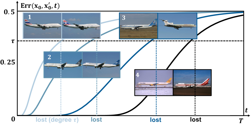
We prove that in the forward diffusion process, each fine-grained is lost at an earlier time-step compared to more coarse-grained , where denotes the set of all class attributes and environmental ones, respectively, and the granularity is defined by the pixel-level changes when altering an attribute. We first formalize the notion of attribute loss, i.e., when an attribute becomes indistinguishable in the noisy images sampled from .
Definition. (Attribute Loss) Without loss of generality, we say that the attribute is lost with degree at when , where is defined as
with and denoting the indicator function. We similarly define the degree of loss for each environmental attribute .
Intuitively, measures the smallest error for a network to reconstruct the original image given noisy ones drawn from or . Hence, when differs from only by , a larger means that the attribute becomes harder to distinguish from , i.e., more severe attribute loss. Particularly, we prove the close-form of in Appendix:
| (5) |
where denotes the error function. Hence we can compute attribute loss at each w.r.t. the pixel-level changes (plotted in Figure 3), allowing us to derive a de-biasing strategy in Section 4.2.
Theorem. 1) For each , there exists a smallest time-step , such that is lost with at least degree at each . This also holds for each . 2) such that whenever is first-order stochastic dominant over with uniformly.
Intuitively, the first part of the theorem states that a lost attribute will not be regained as time-step increases, and there is a time-step when becomes lost (with degree ) for the first time. The second part states that when changing the environmental attribute is more likely to cause a larger pixel-level changes than changing the class attribute , then becomes lost at a larger time-step compared to . See Figure 3 for an illustration of the two parts. We build on this mechanism in Section 4 to removes the visually prominent, yet spurious for de-biasing in FSL.
4 Approach
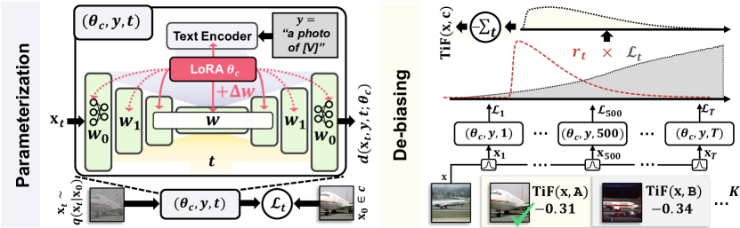
We have shown in Eq. (5) that attribute loss prevents a denoising network to accurately reconstruct from the noisy . Hence by contra-position, if we enable accurate reconstruction by minimizing Eq. (4) using a condition , then the trained network must associate to the lost attributes to make up for their loss (Section 4.1). Moreover, our theorem indicates that only the nuanced is lost at a small time-step , hence is only associated to at , allowing us to remove to de-bias (Section 4.2). We detail our TiF learner below.
4.1 Parameterization
We use the reconstruction loss in Eq. (4) to train a denoising network parameterized by on the few-shot examples of each category by:
| (6) |
When training converges, essentially parameterizes the lost attributes of category at each time-step . We detail our implementation below:
Choice of . We use the text-conditioned Stable Diffusion (SD) [28], as it is trained on internet-scaled data with extensive knowledge of visual attributes. As shown in Figure 4, consists of a text encoder that extracts the text embedding from the prompt , and a U-Net [29] that leverages text and time-step embedding to reconstruct from . Note that SD encodes all images to a latent space. For convenience, we refer to the latent space when we say image, or pixel with a slight abuse of notation.
Choice of . As shown in Figure 4, instead of fine-tuning all the parameters of , we freeze the pre-trained weights of and inject trainable Low-Rank Adaptation (LoRA) matrices to the linear layers in the text encoder and U-Net. For the U-Net, we use a subset of its attention blocks for injecting LoRA (ablation in Section 5.3). For each linear layer with weight , the new weight becomes after injection, where is the injected low-rank matrix. We denote the LoRA matrices parameters for category as . This offers several benefits: 1) The low-rank parameterization limits the model expressiveness to capture only the necessary attributes, e.g., only at a small when is yet lost. 2) As LoRA only affects the attention blocks, the model can only attend to the FSL task using existing visual knowledge, mitigating catastrophic forgetting [16] when adapting to the few-shot examples. 3) This also leads to efficient training and light-weight storage of .
Choice of . We use a fixed text prompt =“a photo of [V]” for all categories, where [V] is a rare token identifier following DreamBooth [30]. The intuition is to choose [V] with a weak semantic prior, such that does not need to detach it from its existing meaning first, before associating it with the specificity of category . Note, it is not necessary to use a different for each , as the LoRA matrices are class-specific and trained separately in Eq. (6).
4.2 De-biasing by Time-steps
Inference Rule. After training, the parameterization enables the denoising network to make up for the lost attributes at for category . For a test image , our TiF learner defines its similarity with a category as the ability of to make up for the lost class attributes (i.e., nuances) in at each , given by:
| (7) |
which enables inference by Eq. (1). Here, is a ratio, namely, the degree of class attribute loss over that of all attribute losses. As shown in Figure 2, highlights the ability of to make up the loss of fine-grained at a small , and essentially disregards the ability to make up the visually prominent by reaching towards 0 at a larger . Hence TiF learner essentially mitigates the influence from to de-bias. We show how to compute below.
Degree of Class Attribute Loss. To compute the degree of class attribute loss using Eq. (5), we need to estimate the average pixel-level changes when only altering the class attributes (measured by L2 distance). A naive way is to directly find the minimum L2 distance between any two images from different categories. However, it is unlikely for the few-shot training set to contain two images that differ only in , e.g., we may have class A on sky, B on ground and C with half sky and half ground. To this end, we estimate by a pixel-level approach:
| (8) |
where denotes the image size, and is the pixel-level value at spatial location . In the earlier example, the sky and ground of C can be matched by with that of A and B, respectively, hence minimizing the influence of background.
| Method | FGVCAircraft | ISIC2019 | |||||||||||
| 1 | 2 | 4 | 8 | 16 | 1 | 2 | 4 | 8 | 16 | ||||
| CLIP | Zero-Shot [26] | 24.9 | 12.5 | ||||||||||
| CoOp [48] | 22.8 -2.1 | 28.4 +3.5 | 32.4 +7.5 | 37.7 +12.8 | 40.5 +15.6 | 10.8 -1.7 | 19.3 +6.8 | 19.6 +7.1 | 24.2 +11.7 | 25.8 +13.3 | |||
| Co-CoOp [47] | 30.1 +5.2 | 31.6 +6.7 | 33.6 +8.7 | 37.3 +12.4 | 38.2 +13.3 | 11.4 -1.1 | 13.9 +1.4 | 16.6 +4.1 | 21.8 +9.3 | 22.8 +10.3 | |||
| MaPLe* [15] | 30.1 +5.2 | 33.0 +8.1 | 33.8 +8.9 | 39.4 +14.5 | 40.7 +15.8 | 11.8 -0.7 | 14.5 +2.0 | 18.0 +5.5 | 22.6 +10.1 | 26.8 +14.3 | |||
| OpenCLIP | Zero-Shot [26] | 42.3 | 16.9 | ||||||||||
| Linear-probe [26] | 18.4 -23.9 | 32.5 -9.8 | 44.1 +1.8 | 55.0 +12.7 | 59.8 +17.5 | 12.4 -4.5 | 14.5 -2.4 | 17.7 +0.8 | 20.1 +3.2 | 21.6 +4.7 | |||
| Tip-Adapter [44] | 47.7 +5.4 | 51.6 +9.3 | 54.7 +12.4 | 58.4 +16.0 | 62.2 +19.9 | 22.6 +5.7 | 25.3 +8.4 | 23.6 +6.7 | 31.1 +14.2 | 33.9 +17.0 | |||
| Tip-Adapter-F [44] | 48.4 +6.1 | 53.9 +11.6 | 56.9 +14.7 | 62.0 +19.7 | 67.4 +25.1 | 21.4 +4.5 | 22.3 +5.4 | 26.8 +9.9 | 34.4 +17.5 | 40.3 +23.4 | |||
| CaFo* [45] | 51.7 +9.4 | 54.6 +12.3 | 58.5 +16.2 | 63.2 +20.9 | 66.7 +24.4 | - | - | - | - | - | |||
| DM | Zero-Shot [17] | 24.3 | 11.7 | ||||||||||
| TiF learner w/o | 40.4 +16.1 | 53.8 +29.5 | 65.0 +40.7 | 72.1 +47.8 | 80.4 +56.1 | 23.9 +12.2 | 26.7 +15.0 | 33.3 +21.6 | 36.5 +24.8 | 43.8 +32.1 | |||
| TiF learner | 48.5 +24.2 | 55.8 +31.5 | 64.2 +39.9 | 74.2 +49.9 | 79.9 +55.6 | 24.1 +12.4 | 27.6 +15.9 | 33.8 +22.1 | 37.2 +25.5 | 44.7 +33.0 | |||
Computing . After obtaining , we compute by
| (9) |
where is the weight term from Eq. (5). In the denominator, we essentially use the integral to simulate diverse environmental attributes that are more coarse-grained than the nuanced class attributes. We include the computation details in Appendix.
5 Experiments
5.1 Settings
Datasets. Our experiments were conducted on four challenging and diverse datasets about fine-grained or customized classes: For fine-grained classification, we used: 1) FGVCAircraft [22] consists of aircraft images from 100 classes with subtle visual differences. 2) ISIC2019 [4, 38] includes a diverse collection of dermatoscopic images with 8 types of skin lesions, serving as a testbed for our model’s performance in medical image analysis. For customized classification, we used re-IDentification (reID) datasets, where each class is a specific identity (e.g., a person or car): 3) DukeMTMC-reID [27] contains 702 person IDs captured by 8 surveillance cameras (for evaluation), and we sub-sampled 150 IDs with the most test images for few-shot evaluation. 4) VeRi-776 [19, 20] contains 200 vehicle IDs under 20 cameras, providing a diverse range of angles and environmental conditions.
Evaluation Details. We followed the protocol in [48, 8] to directly adapt models on the -way--shot few-shot training set. This setting is more versatile with two main differences from the conventional FSL: 1) We did not perform pre-training or meta-learning on a many-shot training set relating with the FSL task [2, 40, 7]. 2) Our ranges from 100 to 200, much larger than the restricting typical in the conventional setting [39, 35]. On FGVCAircraft, we sampled the few-shot set from its train split and evaluated accuracy on its test split. On ISIC2019, as its test split has no ground-truth labels, we sampled few-shot set from the train split and tested on the rest images. We used the macro F1 score to account for the class imbalance. On the reID datasets, we sampled few-shot images from their gallery set, and evaluated (rank-1) accuracy on their query set.
Implementation Details. We used SD 2.0 following [17], as we empirically found that the more commonly used SD 2.1 performs slightly worse in classification (see Appendix). For LoRA matrices rank, we used 8 on ISIC2019 and 16 on the rest datasets by visual inspection of the generation quality (see Section 5.3). We used a fixed rare token identifier [V]=“hta” for all experiments. On dataset with class names, zero-shot CLIP and its adapter uses “a photo of [], a type of [SC]” for each prompt , where [] denotes the name for class and [SC] is a dataset-specific super-class name, i.e., “aircraft” on FGVCAircraft and “skin lesion” on ISIC2019. For fair comparison, we implemented our as “a photo of [V] [], a type of [SC]”. We also tried a variant without using class names (denoted as w/o ) by setting as “a photo of [V], a type of [SC]”. For inference, we modified the implementation in [17] to add our weight in Eq. (9). Other details in Appendix.
Baselines. We used two CLIP variants: CLIP with ViT-B/16 backbone trained on 400M image-caption pairs, and OpenCLIP with ViT-H/14 trained on LAION-2B. We compared with two lines of methods: 1) CLIP-Adapter [8], Tip-Adapter [44] and CaFo [45] based on Eq. (2). 2) Prompt-tuning methods CoOp [48], Co-CoOp [47] and MaPLe [15], which aim to learn in Eq. 2. However, We did not test them on OpenCLIP, as their official implementations are specifically designed for CLIP and difficult to be fairly reproduced on OpenCLIP. We also compared with the zero-shot Diffusion Classifier [17], which is based on SD.
5.2 Main Results
| Method | DukeMTMC-reID | VeRi-776 | |||||||||||
| 1 | 2 | 4 | 8 | 16 | 1 | 2 | 4 | 8 | 16 | ||||
| CLIP | CoOp [48] | 8.2 | 10.4 | 17.2 | 29.6 | 33.7 | 11.4 | 13.9 | 18.1 | 30.3 | 34.1 | ||
| Co-CoOp [47] | 9.7 | 12.1 | 20.1 | 32.7 | 44.5 | 30.1 | 31.6 | 33.6 | 37.3 | 38.2 | |||
| MaPLe [15] | 13.5 | 32.9 | 40.7 | 55.7 | 63.0 | 35.2 | 40.7 | 44.4 | 57.5 | 68.1 | |||
| OC | Linear-probe [26] | 11.9 | 13.2 | 37.7 | 53.5 | 60.2 | 16.7 | 29.5 | 51.1 | 61.1 | 69.8 | ||
| Tip-Adapter [44] | 28.5 | 36.9 | 46.5 | 59.3 | 66.7 | 36.4 | 47.5 | 59.8 | 71.2 | 80.1 | |||
| Tip-Adapter-F [44] | 29.3 | 32.0 | 54.4 | 74.2 | 82.6 | 37.4 | 48.6 | 62.2 | 79.1 | 85.4 | |||
| TiF learner w/o | 36.9 | 53.6 | 73.1 | 83.7 | 91.6 | 41.9 | 60.7 | 78.2 | 91.2 | 96.8 | |||
| Method | FGVCAircraft | DukeMTMC-reID | |||||||||||
|---|---|---|---|---|---|---|---|---|---|---|---|---|---|
| 1 | 2 | 4 | 8 | 16 | 1 | 2 | 4 | 8 | 16 | ||||
| Subset | last | 48.5 | 55.8 | 64.2 | 73.1 | 78.1 | 36.9 | 53.6 | 73.1 | 84.2 | 91.3 | ||
| last + | 48.2 | 55.7 | 65.0 | 74.2 | 78.5 | 28.7 | 47.7 | 69.7 | 84.5 | 91.1 | |||
| last + + | 46.5 | 55.4 | 65.1 | 74.0 | 79.9 | 25.8 | 43.2 | 65.7 | 83.4 | 91.6 | |||
| Weight | ELB weight | 44.7 | 50.2 | 59.9 | 68.7 | 71.2 | 33.2 | 50.2 | 68.5 | 78.3 | 81.8 | ||
| PDAE | 49.2 | 56.7 | 64.1 | 72.2 | 78.1 | 36.2 | 53.9 | 73.4 | 81.2 | 90.8 | |||
| Ours | 48.5 | 55.8 | 64.2 | 74.2 | 79.9 | 36.9 | 53.6 | 73.1 | 84.5 | 91.6 | |||
Overall Results. As shown in Table 1 and 2, our TiF learner achieves state-of-the-art performance across fine-grained and reID datasets, e.g., significantly improving existing methods by 13.7% on FGVCAircraft, 21.6% on DukeMTMC-reID and 16% on VeRi-776. On ISIC2019, we still achieve up to 7% absolute gain over the best-performing baseline, despite the challenges posed by diverse appearances within each class, as well as the stringent macro-F1 evaluation, which is sensitive to under-performing classes. Note that prompt tuning methods generally have non-ideal performances. This holds especially on customized reID classes with no class name to provide semantic prior. This validates the difficulties to describe the specification of fine-grained classes by prompt alone.
Low vs. High Shots. On low-shot settings (e.g., 1- or 2-shot), we observe that our method may not improve significantly. However, not all foundation models are equal, and we must account for the discriminative capability of a zero-shot model. By checking the gain of each method over its zero-shot foundation model (small numbers) in Table 1, we observe that our method improves the most, e.g., by +24.2% with just 1-shot on FGVCAircraft. We also highlight that CaFo leverages an ensemble of multiple models (i.e., CLIP, DALL-E, GPT-3 and DINO), which provides rich prior to enable higher low-shot performance. By increasing #shots, our TiF learner’s accuracy continue to grow strongly, e.g., reaching near perfect predicting on the challenging 200-way-16-shot VeRi-776 task. This validates that our method can reap the benefits from well-defined class attributes using more shots. Moreover, the overall large improvements over baselines on 16-shot also highlights the persistence of spurious correlations, i.e., any attribute from the diverse visual attributes set can spuriously correlate with to challenge a few-shot learner.
With vs. Without []. On fine-grained datasets, we have access to the class name, and can include the class name in our prompt (see implementation details). Hence we compared the performance of TiF learner when using or without using class names (w/o ) in Table 1. On FGVCAircraft, using class names significantly improves the 1- and 2-shot settings. This is because the class names can provide semantic prior to help describe the classes, which are otherwise ill-defined given the extreme low number of training images. However, on ISIC2019, using class names do not help with low-shot settings as much, and we conjecture that the prior knowledge of SD on ISIC2019 is significantly weaker compared to that on FGVCAircraft (much lower zero-shot accuracy). On higher-shot settings, adding class names overall has little to no effect, as the expanded training set can properly define each class.
5.3 Ablations
LoRA Injection Subset. In conventional few-shot learning works [36], it is common to train only the last few layers of the backbone, corresponding to low-level features. As our goal is to capture fine-grained attributes, we are motivated to inject LoRA to the last attention blocks of the SD U-Net, as shown in Figure 4. Starting from just injecting the last block (solid line), we tried expanding the injected blocks and show the results in Table 3 top. On 1-, 2- and 4-shot settings, injecting last attention block brings consistent improvements over other options. We conjecture that this provides additional inductive bias for the model to focus on the fine-grained details (controlled by the last block). However, on 8-shot and 16-shot settings, this becomes suboptimal, and we postulate that this can limit the expressiveness of the injected SD, such that it fails to capture the specification of each class. Overall, “last + ” and “last + + ” work the best for 8- and 16-shot, respectively. Hence we use these settings for all experiments in Table 1 and 2. See additional ablation on this in Appendix.
Inference Weight . In Table 3 bottom, we compared our inference weight in Eq. (9) with two other weights. The ELB weight is derived from the evidence lower bound of the training data distribution (see Appendix), which respects any spurious correlation, e.g., if most airplanes have sky background, the weight will encourage DM to follow this pattern in its generation. Hence it leads to sub-optimal performance when we want to suppress the spurious correlations in FSL. The PDAE weight [46] is developed to help distill visual attribute knowledge from a pre-trained DM, and also penalizes large time-steps when distillation is empirically difficult. Hence overall, it also performs reasonably well. However, it comes with a hyper-parameter , and when we use its default setting , it does not perform well on some settings, e.g., 16-shot on FGVCAircraft. In contrast, our proposed hyper-parameter-free adaptive weight is overall more stable due to its tailored design to isolate nuanced attributes from visually prominent ones.
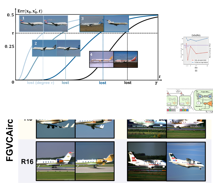
LoRA Rank is the rank of each LoRA matrix . As our method is based on a generative model, we can easily choose its rank through a visual approach on the train set. Specifically, we synthesize images using the LoRA-injected SD. A desired rank should enable SD to generate the specification of each class, but still limits it from overfitting to irrelevant details. As shown in Figure 5, rank 16 on ISIC2019 is too high, as the model overfits to the scratches on the lens, while rank 8 on FGVCAircraft is too low, as the model fails to capture the wing and the vertical stabilizer. Overall, we used rank 8 for ISIC2019 with simpler visual attributes and rank 16 for the rest.
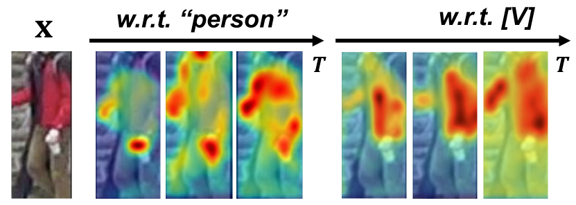
Additional Attention Maps. In Figure 6, we show attention maps on DukeMTMC-reID w.r.t. different input tokens, where “person” corresponds to human parts and “[V]” is associated with the class attribute clothes that uniquely identify this person.
6 Conclusions
We presented TiF learner, a novel few-shot learner parameterization based on the Diffusion Model (DM), leveraging the inductive bias of its time-steps to isolate nuanced class attributes from visually prominent, yet spurious ones. Specifically, we theoretically show that in the forward diffusion process, nuanced attributes are lost at a smaller time-step than the visually prominent ones. Based on this, we train class-specific low-rank adapters that enables a text-conditioned DM to make up for the attribute loss by accurately reconstructing images from their noisy ones given a prompt. Hence each adapter and the prompt parameterizes only the nuanced class attributes at a small time-step, enabling a robust inference rule that focuses on the class attributes. Extensive results show that our method significantly outperforms strong baselines on various fine-grained or customized few-shot learning tasks. As future direction, we will seek additional inductive bias to tackle more complicated scenarios (e.g., hierarchical classification).
7 Acknowledgement
This research is supported by the National Research Foundation, Singapore under its AI Singapore Programme (AISG Award No: AISG2-RP-2021-022), MOE AcRF Tier 2 (MOE2019-T2-2-062), Wallenberg-NTU Presidential Postdoctoral Fellowship, the A*STAR under its AME YIRG Grant (Project No.A20E6c0101) and the Lee Kong Chian (LKC) Fellowship fund awarded by Singapore Management University. Pan Zhou was supported by the Singapore Ministry of Education (MOE) Academic Research Fund (AcRF) Tier 1 grant.
References
- Chen et al. [2023] Haokun Chen, Xu Yang, Yuhang Huang, Zihan Wu, Jing Wang, and Xin Geng. Manipulating the label space for in-context classification. arXiv preprint arXiv:2312.00351, 2023.
- Chen et al. [2019] Wei-Yu Chen, Yen-Cheng Liu, Zsolt Kira, Yu-Chiang Frank Wang, and Jia-Bin Huang. A closer look at few-shot classification. In International Conference on Learning Representations, 2019.
- Cherti et al. [2023] Mehdi Cherti, Romain Beaumont, Ross Wightman, Mitchell Wortsman, Gabriel Ilharco, Cade Gordon, Christoph Schuhmann, Ludwig Schmidt, and Jenia Jitsev. Reproducible scaling laws for contrastive language-image learning. In Proceedings of the IEEE/CVF Conference on Computer Vision and Pattern Recognition, pages 2818–2829, 2023.
- Combalia et al. [2019] Marc Combalia, Noel CF Codella, Veronica Rotemberg, Brian Helba, Veronica Vilaplana, Ofer Reiter, Cristina Carrera, Alicia Barreiro, Allan C Halpern, Susana Puig, et al. Bcn20000: Dermoscopic lesions in the wild. arXiv preprint arXiv:1908.02288, 2019.
- D’Amour [2019] Alexander D’Amour. On multi-cause causal inference with unobserved confounding: Counterexamples, impossibility, and alternatives. In AISTATS, 2019.
- Dhillon et al. [2020] Guneet S Dhillon, Pratik Chaudhari, Avinash Ravichandran, and Stefano Soatto. A baseline for few-shot image classification. In International Conference on Learning Representations, 2020.
- Finn et al. [2017] Chelsea Finn, Pieter Abbeel, and Sergey Levine. Model-agnostic meta-learning for fast adaptation of deep networks. In ICML, 2017.
- Gao et al. [2021] Peng Gao, Shijie Geng, Renrui Zhang, Teli Ma, Rongyao Fang, Yongfeng Zhang, Hongsheng Li, and Yu Qiao. Clip-adapter: Better vision-language models with feature adapters. arXiv preprint arXiv:2110.04544, 2021.
- Gidaris and Komodakis [2019] Spyros Gidaris and Nikos Komodakis. Generating classification weights with gnn denoising autoencoders for few-shot learning. In Proceedings of the IEEE Conference on Computer Vision and Pattern Recognition, 2019.
- Guo et al. [2022] Ziyu Guo, Renrui Zhang, Longtian Qiu, Xianzheng Ma, Xupeng Miao, Xuming He, and Bin Cui. Calip: Zero-shot enhancement of clip with parameter-free attention. In AAAI, 2022.
- Higgins et al. [2018] Irina Higgins, David Amos, David Pfau, Sebastien Racaniere, Loic Matthey, Danilo Rezende, and Alexander Lerchner. Towards a definition of disentangled representations. arXiv preprint arXiv:1812.02230, 2018.
- Ho et al. [2020] Jonathan Ho, Ajay Jain, and Pieter Abbeel. Denoising diffusion probabilistic models. NeurIPS, 2020.
- Hu et al. [2022] Edward J Hu, Yelong Shen, Phillip Wallis, Zeyuan Allen-Zhu, Yuanzhi Li, Shean Wang, Lu Wang, and Weizhu Chen. LoRA: Low-rank adaptation of large language models. In ICLR, 2022.
- Ilharco et al. [2021] Gabriel Ilharco, Mitchell Wortsman, Ross Wightman, Cade Gordon, Nicholas Carlini, Rohan Taori, Achal Dave, Vaishaal Shankar, Hongseok Namkoong, John Miller, Hannaneh Hajishirzi, Ali Farhadi, and Ludwig Schmidt. Openclip, 2021. If you use this software, please cite it as below.
- khattak et al. [2023] Muhammad Uzair khattak, Hanoona Rasheed, Muhammad Maaz, Salman Khan, and Fahad Shahbaz Khan. Maple: Multi-modal prompt learning. In CVPR, 2023.
- Kirkpatrick et al. [2017] James Kirkpatrick, Razvan Pascanu, Neil Rabinowitz, Joel Veness, Guillaume Desjardins, Andrei A Rusu, Kieran Milan, John Quan, Tiago Ramalho, Agnieszka Grabska-Barwinska, et al. Overcoming catastrophic forgetting in neural networks. Proceedings of the national academy of sciences, 2017.
- Li et al. [2023] Alexander C. Li, Mihir Prabhudesai, Shivam Duggal, Ellis Brown, and Deepak Pathak. Your diffusion model is secretly a zero-shot classifier. In ICCV, 2023.
- Liu et al. [2021] Hong Liu, Jianmin Wang, and Mingsheng Long. Cycle self-training for domain adaptation. In NeurIPS, 2021.
- Liu et al. [2016a] Xinchen Liu, Wu Liu, Huadong Ma, and Huiyuan Fu. Large-scale vehicle re-identification in urban surveillance videos. In 2016 IEEE International Conference on Multimedia and Expo (ICME), 2016a.
- Liu et al. [2016b] Xinchen Liu, Wu Liu, Tao Mei, and Huadong Ma. A deep learning-based approach to progressive vehicle re-identification for urban surveillance. In Computer Vision–ECCV 2016: 14th European Conference, Amsterdam, The Netherlands, October 11-14, 2016, Proceedings, Part II 14, 2016b.
- Locatello et al. [2019] Francesco Locatello, Stefan Bauer, Mario Lucic, Gunnar Raetsch, Sylvain Gelly, Bernhard Schölkopf, and Olivier Bachem. Challenging common assumptions in the unsupervised learning of disentangled representations. In ICML, 2019.
- Maji et al. [2013] Subhransu Maji, Esa Rahtu, Juho Kannala, Matthew Blaschko, and Andrea Vedaldi. Fine-grained visual classification of aircraft. arXiv preprint arXiv:1306.5151, 2013.
- Mokady et al. [2023] Ron Mokady, Amir Hertz, Kfir Aberman, Yael Pritch, and Daniel Cohen-Or. Null-text inversion for editing real images using guided diffusion models. In Proceedings of the IEEE/CVF Conference on Computer Vision and Pattern Recognition, pages 6038–6047, 2023.
- Ng and Jordan [2001] Andrew Ng and Michael Jordan. On discriminative vs. generative classifiers: A comparison of logistic regression and naive bayes. NeurIPS, 14, 2001.
- OpenAI [2023] OpenAI. Gpt-4 technical report. arXiv preprint arXiv:2303.08774, 2023.
- Radford et al. [2021] Alec Radford, Jong Wook Kim, Chris Hallacy, Aditya Ramesh, Gabriel Goh, Sandhini Agarwal, Girish Sastry, Amanda Askell, Pamela Mishkin, Jack Clark, et al. Learning transferable visual models from natural language supervision. In ICML, 2021.
- Ristani et al. [2016] Ergys Ristani, Francesco Solera, Roger S. Zou, R. Cucchiara, and Carlo Tomasi. Performance measures and a data set for multi-target, multi-camera tracking. In ECCV Workshops, 2016.
- Rombach et al. [2022] Robin Rombach, Andreas Blattmann, Dominik Lorenz, Patrick Esser, and Björn Ommer. High-resolution image synthesis with latent diffusion models. In CVPR, 2022.
- Ronneberger et al. [2015] Olaf Ronneberger, Philipp Fischer, and Thomas Brox. U-net: Convolutional networks for biomedical image segmentation. In Medical Image Computing and Computer-Assisted Intervention–MICCAI 2015: 18th International Conference, Munich, Germany, October 5-9, 2015, Proceedings, Part III 18, 2015.
- Ruiz et al. [2023] Nataniel Ruiz, Yuanzhen Li, Varun Jampani, Yael Pritch, Michael Rubinstein, and Kfir Aberman. Dreambooth: Fine tuning text-to-image diffusion models for subject-driven generation. In CVPR, 2023.
- Russakovsky et al. [2015] Olga Russakovsky, Jia Deng, Hao Su, Jonathan Krause, Sanjeev Satheesh, Sean Ma, Zhiheng Huang, Andrej Karpathy, Aditya Khosla, Michael Bernstein, et al. Imagenet large scale visual recognition challenge. IJCV, 2015.
- Schölkopf et al. [2021] Bernhard Schölkopf, Francesco Locatello, Stefan Bauer, Nan Rosemary Ke, Nal Kalchbrenner, Anirudh Goyal, and Yoshua Bengio. Toward causal representation learning. Proceedings of the IEEE, 2021.
- Schuhmann et al. [2022] Christoph Schuhmann, Romain Beaumont, Richard Vencu, Cade W Gordon, Ross Wightman, Mehdi Cherti, Theo Coombes, Aarush Katta, Clayton Mullis, Mitchell Wortsman, Patrick Schramowski, Srivatsa R Kundurthy, Katherine Crowson, Ludwig Schmidt, Robert Kaczmarczyk, and Jenia Jitsev. LAION-5b: An open large-scale dataset for training next generation image-text models. In Thirty-sixth Conference on Neural Information Processing Systems Datasets and Benchmarks Track, 2022.
- Selvaraju et al. [2017] Ramprasaath R Selvaraju, Michael Cogswell, Abhishek Das, Ramakrishna Vedantam, Devi Parikh, and Dhruv Batra. Grad-cam: Visual explanations from deep networks via gradient-based localization. In Proceedings of the IEEE International Conference on Computer Vision, 2017.
- Snell et al. [2017] Jake Snell, Kevin Swersky, and Richard Zemel. Prototypical networks for few-shot learning. In Advances in Neural Information Processing Systems, 2017.
- Sun et al. [2019] Qianru Sun, Yaoyao Liu, Tat-Seng Chua, and Bernt Schiele. Meta-transfer learning for few-shot learning. In CVPR, 2019.
- Tang et al. [2020] Hui Tang, Ke Chen, and Kui Jia. Unsupervised domain adaptation via structurally regularized deep clustering. In CVPR, 2020.
- Tschandl et al. [2018] Philipp Tschandl, Cliff Rosendahl, and Harald Kittler. The ham10000 dataset, a large collection of multi-source dermatoscopic images of common pigmented skin lesions. Scientific data, 2018.
- Vinyals et al. [2016] Oriol Vinyals, Charles Blundell, Timothy Lillicrap, Daan Wierstra, et al. Matching networks for one shot learning. In Advances in Neural Information Processing Systems, 2016.
- Wertheimer et al. [2021] Davis Wertheimer, Luming Tang, and Bharath Hariharan. Few-shot classification with feature map reconstruction networks. In CVPR, 2021.
- Yue et al. [2020] Zhongqi Yue, Hanwang Zhang, Qianru Sun, and Xian-Sheng Hua. Interventional few-shot learning. In NeurIPS, 2020.
- Yue et al. [2023] Zhongqi Yue, Hanwang Zhang, and Qianru Sun. Make the u in uda matter: Invariant consistency learning for unsupervised domain adaptation. In NeurIPS, 2023.
- Zhang et al. [2020] Chi Zhang, Yujun Cai, Guosheng Lin, and Chunhua Shen. Deepemd: Few-shot image classification with differentiable earth mover’s distance and structured classifiers. 2020.
- Zhang et al. [2022a] Renrui Zhang, Rongyao Fang, Peng Gao, Wei Zhang, Kunchang Li, Jifeng Dai, Yu Qiao, and Hongsheng Li. Tip-adapter: Training-free clip-adapter for better vision-language modeling. In ECCV, 2022a.
- Zhang et al. [2023] Renrui Zhang, Xiangfei Hu, Bohao Li, Siyuan Huang, Hanqiu Deng, Hongsheng Li, Yu Qiao, and Peng Gao. Prompt, generate, then cache: Cascade of foundation models makes strong few-shot learners. In CVPR, 2023.
- Zhang et al. [2022b] Zijian Zhang, Zhou Zhao, and Zhijie Lin. Unsupervised representation learning from pre-trained diffusion probabilistic models. NeurIPS, 2022b.
- Zhou et al. [2022a] Kaiyang Zhou, Jingkang Yang, Chen Change Loy, and Ziwei Liu. Conditional prompt learning for vision-language models. In CVPR, 2022a.
- Zhou et al. [2022b] Kaiyang Zhou, Jingkang Yang, Chen Change Loy, and Ziwei Liu. Learning to prompt for vision-language models. IJCV, 2022b.
- Zhu et al. [2023] Beier Zhu, Yulei Niu, Yucheng Han, Yue Wu, and Hanwang Zhang. Prompt-aligned gradient for prompt tuning. International Conference on Computer Vision, 2023.