Real-time portable muography with Hankuk Atmospheric-muon Wide Landscaping : HAWL

Abstract

Cosmic ray muons prove valuable across various fields, from particle physics experiments to non-invasive tomography, thanks to their high flux and exceptional penetrating capability. Utilizing a scintillator detector, one can effectively study the topography of mountains situated above tunnels and underground spaces. The Hankuk Atmospheric-muon Wide Landscaping (HAWL) project successfully charts the mountainous region of eastern Korea by measuring cosmic ray muons with a detector in motion. The real-time muon flux measurement shows a tunnel length accuracy of 6.5 %, with a detectable overburden range spanning from 8 to 400 meter-water-equivalent depth. This is the first real-time portable muon tomography.

[1]organization=Department of Physics, Chung-Ang University,city=Seoul, postcode=06974, country=Republic of Korea

[2]organization=Physics Institute, University of São Paulo,city=São Paulo, postcode=05508-090, country=Brazil

1 Introduction

A cosmic-ray muon is an elementary particle generated when a primary cosmic-ray particle collides with atmospheric nuclei Workman et al. (2022). Cosmic-ray muons, in abundance, can traverse high-density materials non-destructively, and their unique energy loss in a material renders them valuable in various applications, from particle physics experiments to muon tomography. In particle physics experiments, a high spatial and temporal resolution muon counter can measure muon flux, track final state particles in an accelerator beam Hewes et al. (2021), and reveal yearly modulations with zenith angle dependence Tilav et al. (2020). Muon tomography has uncovered unknown spaces within pyramids Procureur et al. (2023b) and is employed to assess the condition of nuclear power plants Procureur et al. (2023a). Furthermore, recent advancements in high-resolution muon imaging technology and portable detectors have broadened their applications, notably in volcanic activity detection Tioukov et al. (2019) and archaeological site investigations Avgitas et al. (2022).

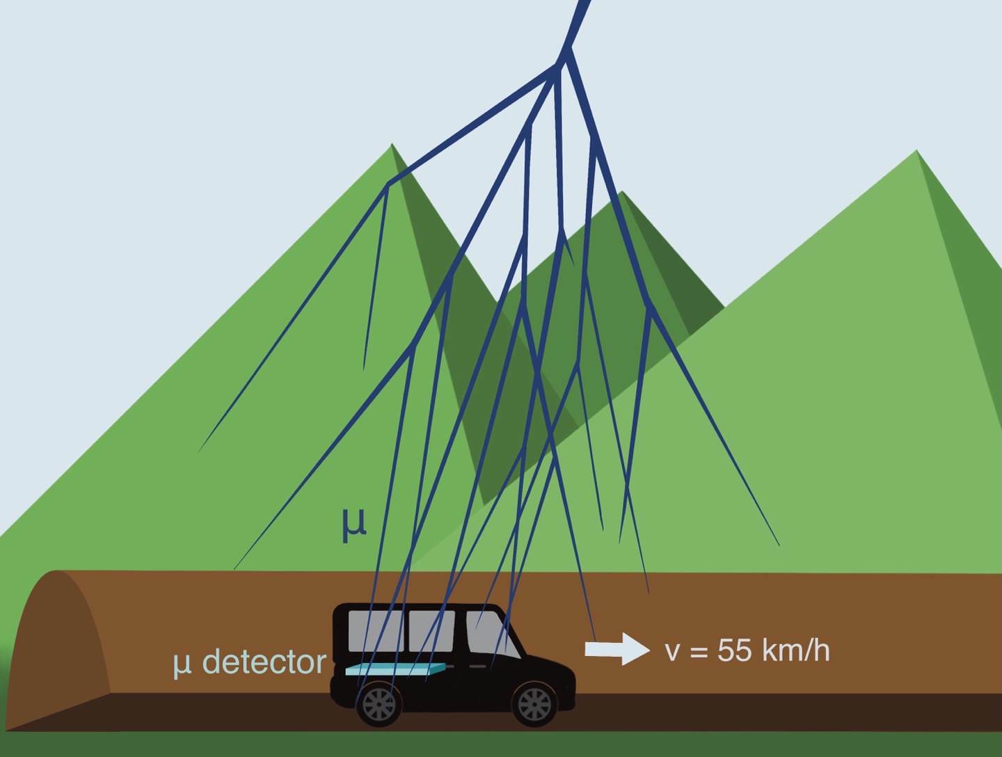
Figure 1: Schematic diagram of the HAWL tomography measurement. The cosmic-ray muon flux is measured in real-time by the HAWL detector loaded in a moving vehicle. The change in the flux relative to the open area can represent the vertical overburden of the rock above the detector.

The primary goal of this research is to map the land forms and features above the underground spaces quickly and non-invasively using a moving muon detector. To reconstruct mountainous topography using measured muon flux, we launched the Hankuk Atmospheric-muon Wide Landscaping (HAWL) project. HAWL precisely gauges changes in muon flux within tunnels situated above the Seoul-Yangyang highway and Yangyang Underground Laboratory (Y2L) Adhikari et al. (2018a) in South Korea while moving in high speed as schematically shown in Fig. 1. With data collected by the HAWL detector, we measured the muon flux as a function of elevation, and the detector sensitivity in terms of depth and length resolutions for the tunnels.

2 Experimental Method

The main design goal of the HAWL experiment is to be compact to fit in a vehicle and to be simply-integrated to consume low power. We chose the plastic scintillator (PS) as the main detection medium which is durable in rough conditions and relatively easy to handle Knoll (2010). To be efficient in power and space usage, small-sized silicon photomultipliers (SiPMs) coupled with optical fibers are used for the light sensor. A customized data acquisition system is developed to make the overall data processing easily streamlined.

2.1 Detector Construction

The muon counter is constructed from rectangular PS material (Eljen Technology, EJ-200) Eljen (2023) with dimensions of $\rm 490~{}mm\times 600~{}mm\times 30~{}mm$. A total of 56 optical fibers coupled with 28 SiPMs are laid out as a grid on the top and bottom surfaces of the PS material.

The cylindrical fiber (Kuraray, double-cladding Y-11) Kuraray (2024) is a wavelength-shifting scintillator with 1 mm diameter that has an absorption peak at 430 nm and an emission peak at 476 nm with an attenuation length greater than 3.5 m. The SiPM (Hamamatsu, S13360-1375PE) MPPC (2024) consists of 285 pixels and has a gain of $4.0\times 10^{6}$ in a $\rm 1.3\times 1.3~{}mm^{2}$ photosensitive area. Six SiPMs are placed on short sides and eight on long sides. The arrangement included 56 optical fibers crossing each other at 19 mm intervals on both the top and bottom of the PS scintillator with 4 ends of optical fibers joined together to couple one SiPM. For optimal performance, the tip of each optical fiber was polished, and a small amount of optical grease was applied at the junction between the SiPM and the optical fiber ends.

To better couple the tip of the optical fibers on a SiPM sensitive area, a fixture as shown in Fig. 2 is installed to the SiPM front-end board. The optical fiber fixture has a hole with a diameter of 4.0 mm and a vertical depth of 8.0 mm stabilizing the fiber bundle and providing better contact to the sensor.

To prevent leakage of scintillation photons and block external photons, the panel with fibers is first wrapped in a Tyvek sheet which has more than 90 % reflectivity in the scintillation spectrum Janecek (2012) and then is covered by a layer of 50 $\rm\mu m$-thick aluminum foil. A layout of the detector is shown in Fig. 2 and its construction procedures are displayed in Fig. 3.

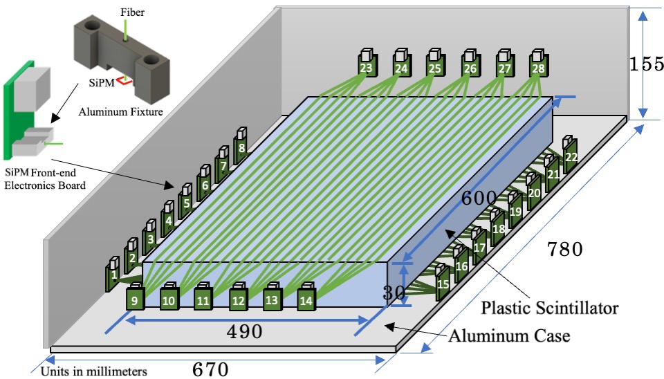
Figure 2: The HAWL detector design. The optical fibers are laid out on top and bottom of a PS panel and their ends are coupled with 28 SiPM light sensors. A SiPM is mounted on a front-end electronics board which sends signals to DAQ via LAN cables. A fixture aids the coupling between the SiPM sensitive area and the tip of the optical fibers. The entire setup is encased in an aluminum housing.

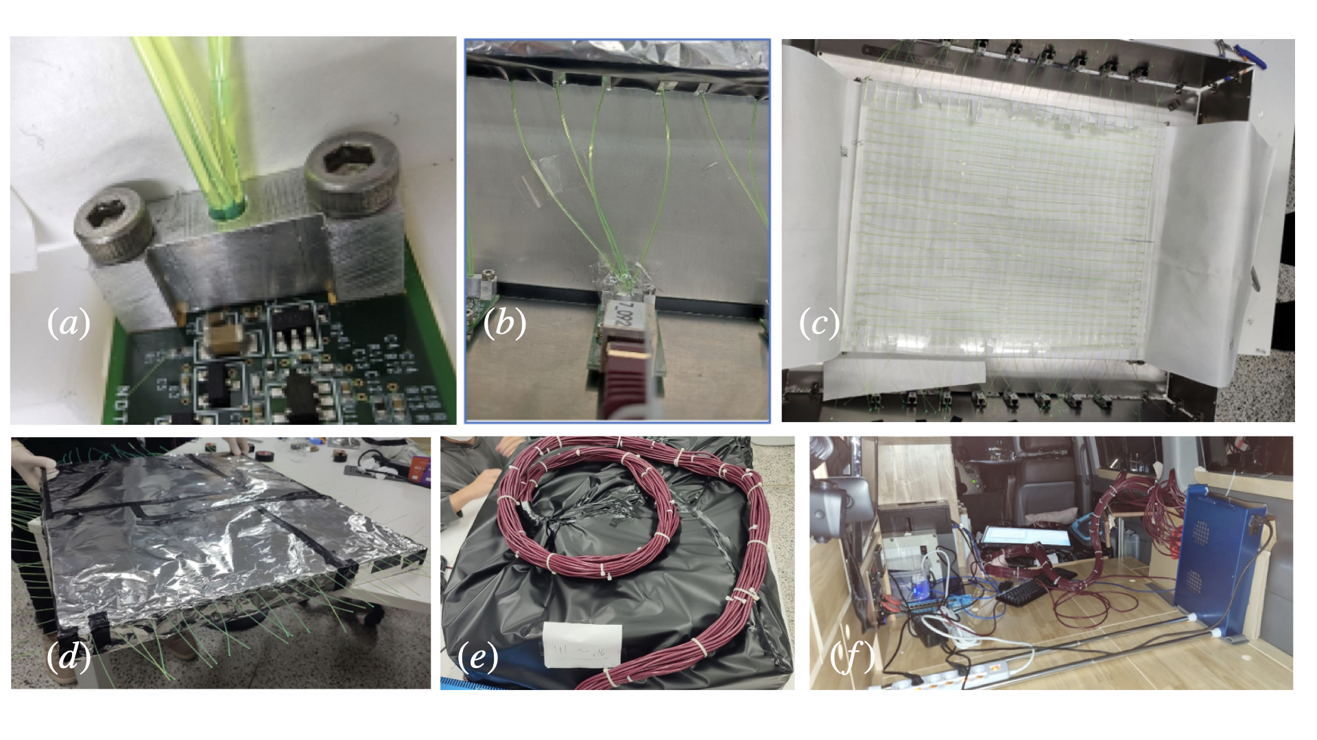
Figure 3: Photos of the HAWL detector assembly. A front-end board connected with four fiber ends are shown in (a) and (b). The layout of the fibers with Tyvek sheets and additional aluminum foil covers are visible in (c) and (d), respectively. The completed HAWL detector is seen in (e) and it is set in place in a van (f) with other DAQ system.

2.2 Data Acquisition

The data acquisition system consists of slow analog to digital converter (SADC), trigger–clock board (TCB) and a desktop computer Adhikari et al. (2018b). The 28 SiPM front-end boards are connected to a custom-made SADC module via a LAN connector. The SADC module provides required voltages to each channel and digitizes the analog signals. The SADC uses 16 ns sampling and has two modes; full waveform mode and sum charge mode. In the waveform mode, all 40-channel waveforms per event are stored while in the sum charge mode, reduced information consisting of only integrated ADC values and average time values for each channel are stored. Example waveforms for the same signal event are shown in Fig. 4.

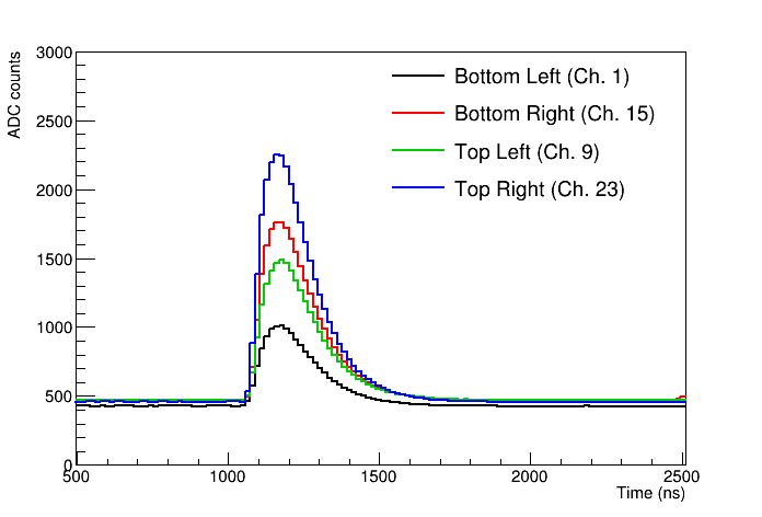
Figure 4: SiPM raw waveform data. Four signal waveforms selected from each side of the detector are displayed. Baselines are typically set around 500 ADC and the amplitude can go up to 4096 ADC. The trigger time starts around 1000 ns and readout window goes to 4096 ns.

The time synchronization and trigger decision are performed by the TCB which is connected to the SADC module via a USB cable. A channel hit is defined when a SiPM signal exceeds the preset threshold level on that channel. A trigger is then formed if 8 or more hits out of 28 active channels are recorded within a 1000 ns time window and an event is constructed by padding the trigger time around 4 $\mu$s readout window aligning the trigger hit times near 1.2 $\mu$s.

The collected raw data is a binary format which is immediately converted into a ROOT format Brun and Rademakers (1997). The detector tests are done in a waveform mode where the trigger settings and the individual channel signal analysis are determined in advance. Then, those conditions are applied to the real-time physics runs using a sum charge mode to minimize the power and disc space loads.

The completed detector has been tested in a lab to set a muon selection cut and check the stability before beginning the physics run collections. Figure 5 shows event distributions in terms of their measured charge. Muons are well separated from the environmental gamma background. A Landau function plus a linear function was used to model the data for muon and gamma components, respectively. A muon selection cut was set at 95 % signal efficiency, allowing 10 % gamma contamination. Subsequently, all equipment was loaded onto the vehicle with a battery. The total power consumption was measured to be 100 Watts. The real-time monitoring was established, allowing results to be broadcasted via wifi. The lab test at 18 m above sea level shows a muon flux of 149.8 events $\rm/m^{2}/s$.

Figure 5: Muon event selection. The rate measurements in a open space are shown as a function of 28-SiPM sum charge. Data are fit to a model defined by an exponential component for environmental radiation (green fills) plus a Landau component for cosmic-ray muons (yellow fills). The vertical dotted line at 15000 ADC is the cut to select muon events.

Muon flux measurements commenced with the portable HAWL detector on November 25, 2022. The trip began from the Gapyeong service area which is located approximately 60 km east of Seoul in the Seoul-Yangyang national highway and traveled to the easterly direction. The muon event rate as a function of time has been displayed in a car. At the same time, the same event rate is broadcasted in real-time by Internet so that it can be simultaneously monitored remotely. To record the speed of the car and the locations of tunnels, we kept camera recording using a smart phone.

The campaign is divided into three sections based on their geographical uniqueness. The section I consists of many tunnels of varying lengths and types while the section II includes the longest tunnel. We enter Yangyang underground laboratory (Y2L) which is the 700 m deep facility that can be accessed by a car in the section III. These sections covered about 100 km out of the total length of the 150 km highway as shown in Fig. 6. We maintained the speed at 55 km/h (the highway lanes have low speed limit of 50 km/h).

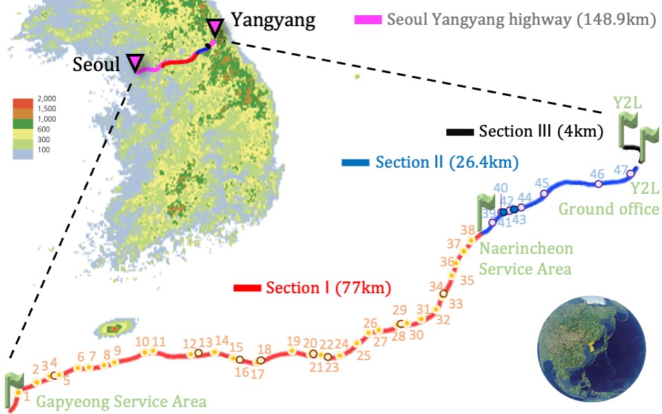
Figure 6: Measurement campaign sections and tunnels. The trip was divided into three sections (I,II, and III). Section I (red line) is from Gapyeong service area to Naerincheon service area and Section II (blue line) is to Y2L ground office. Section III (black line) is on a local road from Y2L ground office to Y2L underground lab. Tunnels are numbered in sequence. The specification of each tunnel can be found in Table 1.

3 Analysis and Results

Physics data of 10822 seconds have been collected and divided in three sections (run-times are 5259 s, 2475 s, and 3088 s, respectively for section I, II, and III). The raw trigger rate was measured at 1901.5 Hz and the rate was reduced to 52 Hz after the cosmic-ray muon selection cut in Fig 5. The moment the van enters a tunnel, the HAWL detector was able to show the muon rate decrease visually as displayed in Fig. 7 and in a video of the Supplementary material.

Figure 7 show the muon event rates as a function of time for the three section measurements. The HAWL detector was able to delineate all tunnels, overpasses, and features above the moving car. The average muon rate was measured at $53.0\pm 0.1$ Hz throughout the campaign. it became reduced to a certain amount when passing a tunnel depending on its length and depth. The section-II includes the 11 km-long tunnel (Inje-Yangyang tunnel) where the maximum vertical overburden is 440 m. For the third section, we recorded the muon rate for the Yangyang underground space. Data show a clear suppression in rates inside the tunnels where we were able to measure the tunnel width and a maximum depth of overburden.

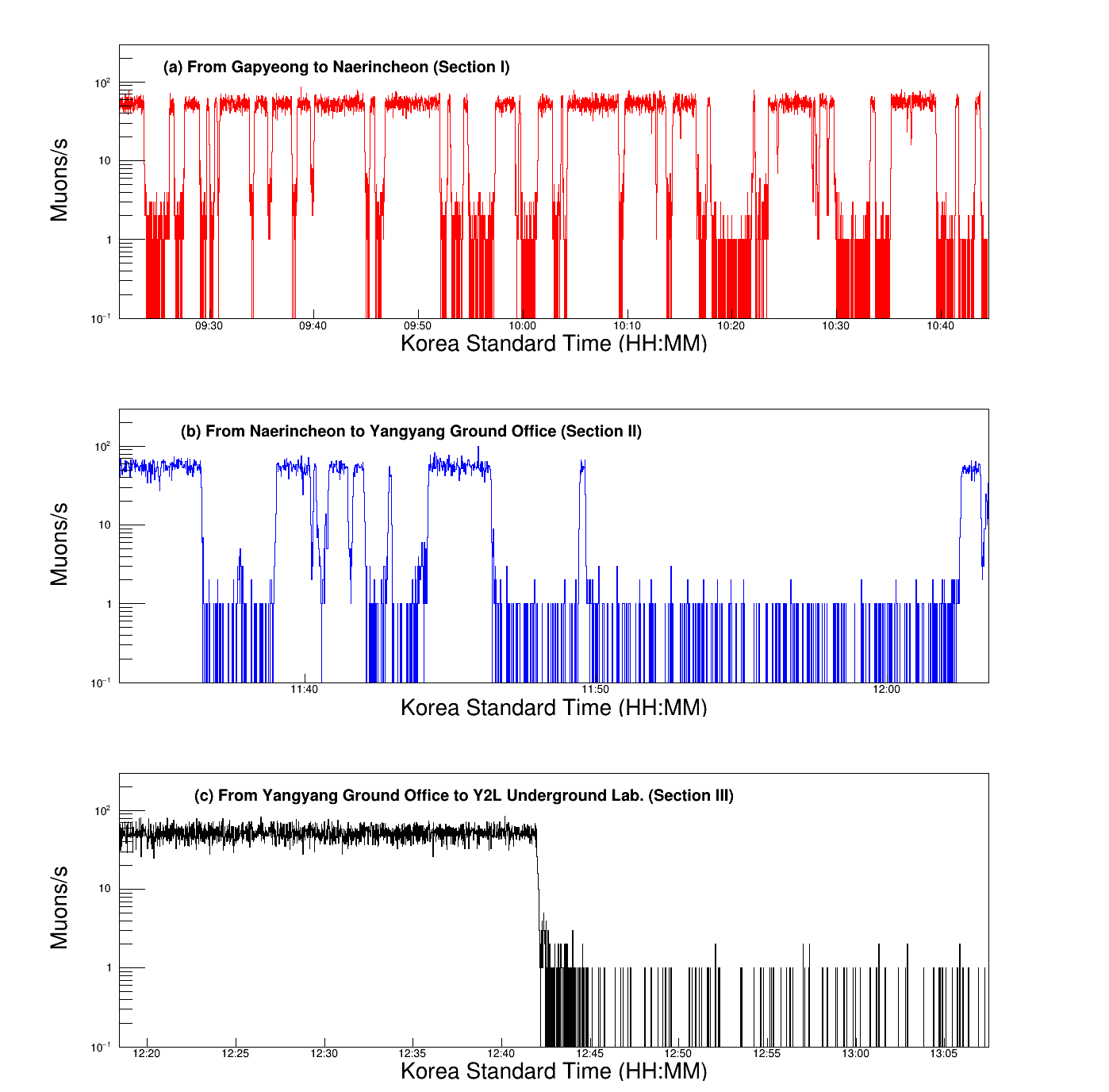
Figure 7: Muon flux measurement campaign. Muon count rates per second is displayed in Section I(a), II(b), and III(c). The rate drops are shown when passing tunnels. Note that the low count rates at deep tunnels in plot (b) and plot (c) appear to be mostly gamma background events.

We model the muon flux reduction based on the extended Sigmoid function $f(t)$ which is defined by

$$f(t)=\frac{A}{1+e^{b(t-m)}}+\frac{A}{1+e^{-b(t-m-w)}}+d,$$ (1)

where $A$ describes open area muon rate, $b$ models the slope of the mountain, $m$ and $w$ represent entrance and width of the tunnel, respectively, and $d$ is the depth parameter. The first term of Eq. 1 is for the entrance side of the tunnel while the second term is mirror reflection for the exiting side. The data segments that show rate reductions were fitted with Eq. 1 using the $\chi^{2}$ minimization to get the best-fit parameters and their uncertainties. An example fit is shown in Fig. 8.

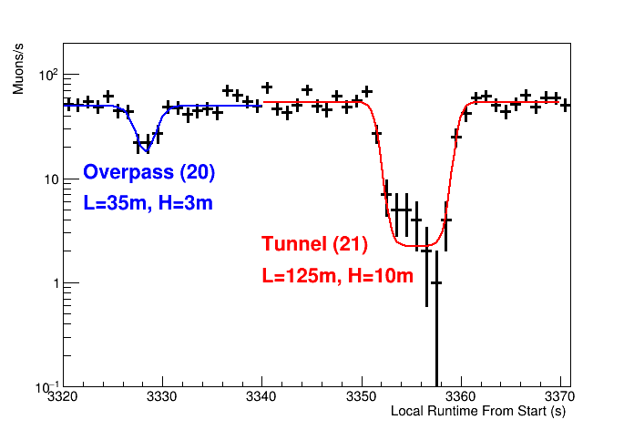
Figure 8: Short tunnel measurements. Two short tunnels are fitted separately. The blue fit line is for the 35 m-long animal overpass with height of 3 m while the red fit line is for the 125 m-long tunnel with maximum height of 10 m.

The fitting results show correct identification of all tunnels when we compared our measurements with the original civil engineering data and satellite images. The short overpasses are identified with limited data points which are constrained by the speed of the vehicle and the size of the detector. A model fit based on the Eq. 1 reveals continuous measurements of the muon flux in open spaces in between the tunnels. Because the highway has been built on an increasing slope (maximum elevation difference is about 400 m) towards the end of the section I and II and a decreasing slope at the end of section II, the muon rate appears to follow the similar characteristics of the elevation. Figure 9 shows the muon flux in an open space as a function of elevation. A constant muon flux model is rejected at more than 5 standard deviation. The correlation coefficient $R=0.72$ between the muon flux and engineering elevation data has been obtained supporting the flux increase as a function of the altitude.

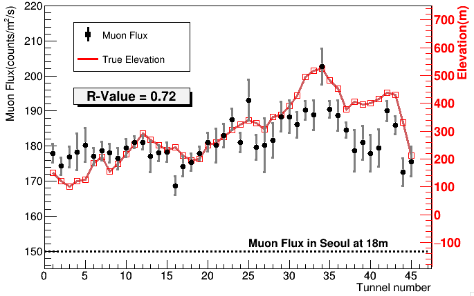
Figure 9: Muon flux as a function of the tunnel location. The muon rate is closely following the elevation changes of the Seoul-Yangyang highway. The correlation coefficient is measured to be $R=0.72$. Please note that the dotted line is reference muon flux measured at 18 m above sea level with the same detector.

Assuming the constant speed of the car at 55 km/h, we estimated the tunnel entrance location and the width as shown in Fig. 10. The width accuracy was measured as 6.5 % by the spread of the relative difference between the measured and true length. The three shortest structures detected were animal overpasses that have lengths of 35 m, 40 m, and 60 m each with 3 m, 3 m, and 5.5 m overburden, respectively.

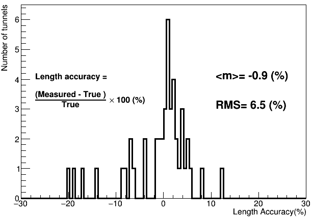
Figure 10: Length accuracy distribution. The relative difference between measured and actual lengths of tunnels is drawn. The accuracy is measured to be 6.5 % while the bias is -0.9 %. The length accuracy is driven by the outliers which are mostly short tunnels.

The muon rates inside the tunnels have been measured as a function of their true maximum depths. Assuming the metamorphic rock contents ($\rho=2.7\,g/cm^{3}$) in northeastern Korean provinces, the depth is converted into the meter-water-equivalent depth. Figure 11 shows the expected exponential reduction behavior Workman et al. (2022). The minimum overburden that data recorded is 3 meters while the maximum overburden is determined at 150 meters which was estimated by the kink in the decay of the data points. The tunnel specifications and measured values are tabulated in Table 1.

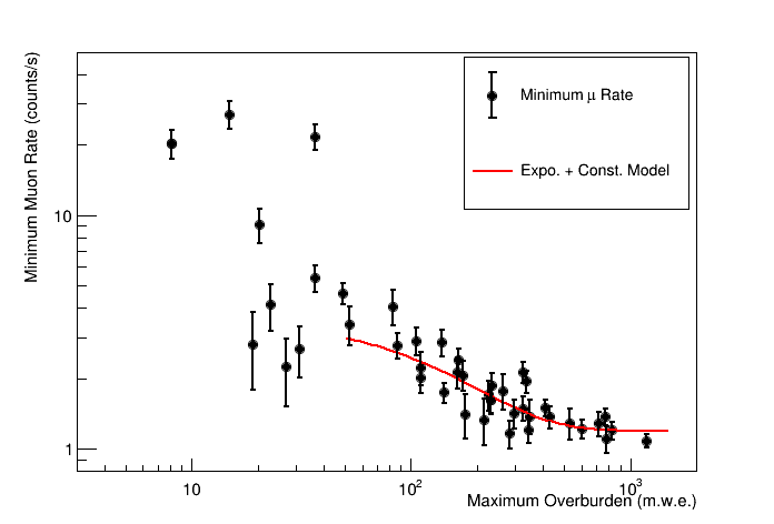
Figure 11: Measured minimum muon rate as a function of true maximum overburden in the meter-water-equivalent (m.w.e.) unit. The muon rate drops exponentially until it is saturated by the gamma contamination. Above 400 m.w.e deep tunnel, the events are dominated by the background gammas.

4 Discussion and Conclusion

The primary challenge lies in acquiring muon data more efficiently, especially considering the speed limits on highways and therefore, a bigger size panel is preferable. Secondly, the separation power between the environmental gammas and muons determines the depth resolution. A detailed analysis after the return of the trip shows most of those events recorded under deeper tunnels (i.e. depth larger than 150 meters) are dominated by gamma background events. Due to the relatively fast speed of the car and the small area detector, it is not efficient to collect a large amount of muon data in a deeper tunnel. On the other hand, we were able to map the short-to-medium tunnels with better accuracy thanks to high count rates. For example, data show that the entrance or exit of the tunnels can be measured with a high precision which helps determine the length of the tunnel. The steepness of mountains near the entrance or exit of the tunnels could be estimated utilizing the slope parameter in the fit. However, to measure the depths more accurately, a tighter control of environmental gamma ray interactions and a larger detector that can collect enough counts are needed.

The HAWL portable muon detector, utilizing a plastic scintillator, was successfully developed to create a mountainous topography, demonstrating muon flux variations based on rock thickness. The completed test validated the detector’s functionality, particularly evident in the expected decrease in muon flux when passing through a tunnel beneath a mountain in the eastern Korea. Analyzing muon flux data along the Seoul-Yangyang highway revealed a close alignment with anticipated tunnel dimensions and tomography above it, achieving a length accuracy of 6.5 % for tunnels at depths ranging from 8 to 400 m.w.e. The HAWL detector demonstrated its unique capability to measure muon rates, while in motion. An upgraded version of HAWL is in development, featuring two thicker panel detectors with anti-coincidence and directional sensitivity. Given its versatility in shallow-depth applications, the HAWL detector is planned to be used in subway systems and underwater tunnels to enhance safety measures.

5 Acknowledgments

This work was supported by National Research Foundation of Korea (NRF) grant funded by the Korean government (MSIT) (NRF-2021R1A2C1013761) and under the framework of international cooperation program managed by the National Research Foundation of Korea (NRF-2021K2A9A1A0609413312), Republic of Korea; Grant No. 2021/06743-1, 2022/12002-7 and 2022/13293-5 FAPESP, CAPES Finance Code 001, CNPq 304658/2023-5 and 303122/2020-0, Brazil.

Table 1: Tunnel specifications and HAWL measurements. Lengths (L) and maximum depths (H) are obtained from engineering blueprints. The elevations are an average value Measured L is equal to the fit width parameter $w$ multiplied by the speed $\rm 55~{}km/h$.

No.	Name	L (m)	Max. H (m)	Elev. (m)	Meas. L(m)	Depth H(/s)	$\mu$ Flux($\rm/m^{2}/s$)
1	Misa	2171	284	155	2218.3	1.37	177.9
2	Magok	919	85	124	914.0	1.62	174.3
3	Balsan 1	633	84	106	633.9	1.70	176.9
4	Balsan 2	480	97.5	126	460.6	1.77	178.3
5	Balsan 3	254	30.5	129	211.2	4.07	180.3
6	Balsan 4	433	60.5	189	435.4	2.13	177.0
7	Chugok	433	32	211	428.5	2.78	178.6
8	Haengchon	463	63.5	160	488.4	2.06	178.0
9	Gwangpan	358	18	186	360.9	4.64	176.4
10	Gunja 1	474	51	220	483.8	2.86	179.4
11	Gunja 2	885	120	255	891.4	2.12	181.1
12	Dongsan 1	680	86	295	689.7	1.87	181.0
13	Dongsan 2	1113	120.5	273	1168.8	1.49	177.0
14	Bukbang 1	2307	152	252	2391.6	1.50	178.0
15	Bukbang 2	326	65	235	328.2	1.41	178.3
16	Bukbang 3	1518	159	246	1550.1	1.37	168.7
17	Hwachon 1	721	85	216	724.0	1.62	174.2
18	Hwachon 2	378	80	200	396.6	1.33	175.4
19	Hwachon 3	527	61	204	522.9	2.39	177.9
20	Hwachon 4	35	3	252	36.3	20.4	181.1
21	Hwachon 5	125	10	264	123.4	2.24	180.2
22	Hwachon 6	629	41	283	606.0	2.01	183.0
23	Hwachon 7	40	3	308	37.5	20.3	182.7
24	Hwachon 8	978	124	328	987.2	1.94	181.0
25	Hwachon 9	3705	304	342	3764.1	1.20	193.1
26	Naechon 1	1261	52.5	332	1155.6	1.74	179.7
27	Naechon 2	88	7.5	309	86.8	9.12	180.2
28	Naechon 3	135	8.5	354	151.3	4.14	181.6
29	Naechon 4	355	39	362	365.8	2.90	188.4
30	Naechon 5	205	19.5	393	176.7	3.42	188.4
31	Seoseok	3061	221.5	430	3183.2	1.22	186.1
32	Haengchiryeong	1422	104	497	1434.9	1.16	190.2
33	Sangnam 1	60	5.5	520	48.1	27.1	190.0
34	Sangnam 2	115	13.5	527	105.3	21.7	201.7
35	Sangnam 3	1719	126.5	485	1714.6	1.20	190.5
36	Sangnam 4	1434	195	454	1472.3	1.29	188.7
37	Sangnam 7	2278	264	381	2342.6	1.28	184.6
38	Girin 1	114	7	408	92.7	2.81	178.7
39	Girin 2	397	41	398	370.4	2.23	181.0
40	Girin 3	162	11.5	402	163.4	2.68	177.9
41	Girin 4	750	128.5	418	765.1	1.38	179.5
42	Girin 5	1148	109.5	441	1165.3	1.42	190.0
43	Girin 6	2665	288.5	432	2785.4	1.10	186.0
44	Inje-Yangyang	10962	440	335	11821.4	1.08	172.5
45	Seomyeon 2	248	13.5	217	230.5	5.38	175.6

References

- Adhikari et al. (2018a) Adhikari, G., et al., 2018a. Initial Performance of the COSINE-100 Experiment. Eur. Phys. J. C 78, 107. doi:10.1140/epjc/s10052-018-5590-x, arXiv:1710.05299.
- Adhikari et al. (2018b) Adhikari, G., et al. (COSINE-100), 2018b. The COSINE-100 Data Acquisition System. JINST 13, P09006. doi:10.1088/1748-0221/13/09/P09006, arXiv:1806.09788.
- Avgitas et al. (2022) Avgitas, T., Elles, S., Goy, C., Karyotakis, Y., Marteau, J., 2022. Muography applied to archaelogy, in: 27e édition de la Réunion des Sciences de la Terre. arXiv:2203.00946.
- Brun and Rademakers (1997) Brun, R., Rademakers, F., 1997. ROOT - An Object Oriented Data Analysis Framework. Nuclear Instruments and Methods in Physics Research Section A: Accelerators, Spectrometers, Detectors and Associated Equipment 389, 81.
- Eljen (2023) Eljen, 2023. Eljen Technology, GENERAL PURPOSE EJ-200, EJ-204, EJ-208, EJ-212. URL: https://eljentechnology.com/products/plastic-scintillators/ej-200-ej-204-ej-208-ej-212.
- Hewes et al. (2021) Hewes, V., et al. (DUNE), 2021. Deep Underground Neutrino Experiment (DUNE) Near Detector Conceptual Design Report. Instruments 5, 31. doi:10.3390/instruments5040031, arXiv:2103.13910.
- Janecek (2012) Janecek, M., 2012. Reflectivity spectra for commonly used reflectors. IEEE Transactions on Nuclear Science 59, 490–497. doi:10.1109/TNS.2012.2183385.
- Knoll (2010) Knoll, G.F., 2010. Radiation detection and measurement. John Wiley and Sons, New York.
- Kuraray (2024) Kuraray, 2024. Plastic scintilating fibers (PSF). URL: https://www.kuraray.com/products/psf.
- MPPC (2024) MPPC, 2024. MPPC for precision measurement, S13360-1375PE. URL: https://www.hamamatsu.com/eu/en/product/optical-sensors/mppc.
- Procureur et al. (2023a) Procureur, S., et al., 2023a. 3D imaging of a nuclear reactor using muography measurements. Science Advances 9, eabq8431.
- Procureur et al. (2023b) Procureur, S., et al., 2023b. Precise characterization of a corridor-shaped structure in Khufu’s Pyramid by observation of cosmic-ray muons. Nature Communications 14, 1144.
- Tilav et al. (2020) Tilav, S., Gaisser, T.K., Soldin, D., Desiati, P. (IceCube), 2020. Seasonal variation of atmospheric muons in IceCube. PoS ICRC2019, 894. doi:10.22323/1.358.0894, arXiv:1909.01406.
- Tioukov et al. (2019) Tioukov, V., et al., 2019. First muography of Stromboli volcano. Scientific Reports 9, 6695.
- Workman et al. (2022) Workman, R., et al. (Particle Data Group), 2022. The Review of Particle Physics. Prog. Theor. Exp. Phys. 2022, 083C01.