TinyGC-Net: An Extremely Tiny Network for Calibrating MEMS Gyroscopes

Abstract

As the errors of microelectromechanical system (MEMS) gyroscopes are complex and nonlinear, the current calibration methods, which rely on linear models or networks with numerous parameters, are inadequate for low-cost embedded computing platforms to achieve both precision and real-time performance. In this paper, we introduce a extremely tiny network (TGC-Net) that characterizes the measurement model of MEMS gyroscopes. The network has a small number of parameters and can be trained on a central processing unit (CPU) before being deployed on a microcontroller unit (MCU). The TGC-Net leverage the robust data processing capabilities of deep learning to derive a nonlinear measurement model from fragmented gyroscope data. Subsequently, this model is used to regress errors on the gyroscope data. Moreover, we analyze the relationship between the compact network and the traditional linear model for MEMS gyroscopes, and emphasize the significance of the adequate angular motion stimulation for train the network. The experimental results, based on public datasets and real-world scenarios, demonstrate the practicality and effectiveness of the proposed method. These findings suggest that this technique is a viable candidate for applications that require MEMS gyroscopes.

• March 2024

Keywords: Gyroscope calibration, deep neural network, orientation estimation, autonomous systems navigation.

1 Introduction

Hello[1]. Inertial measurement units (IMUs) based on Microelectromechanical systems (MEMS), with their attributes of low power consumption, small size, and affordable price, has played a crucial role in various fields such as robotics, smartphones, wearable devices, and virtual reality. To reduce costs, the manufacturers of the MEMS IMU have only performed a rough calibration for their production. So MEMS IMU should be calibrated appropriately before being used. Typically, IMU is composed of a tri-axis gyroscope to measure the carrier’s angular velocity in the body coordinate frame relative to the inertial coordinate frame, and a tri-axis accelerometer to sense the carrier’s acceleration based on Newton’s law and Hooke’s law. The calibration of MEMS IMU has received extensive attention and in-depth research from the open-source community, and many researchers are committed to developing efficient and accurate calibration methods and algorithms to improve the measurement accuracy and reliability of sensors. Due to the fact that their calibration methods are typically based on stable static measurement values, the calibration process for accelerometers is generally simpler and has achieved good results, as well as good practicality and applicability. As the self-rotation angle velocity of the earth is weak and buried in measurement noise, so more external reference excitation is a prime requisite for calibrating a consumer grade gyroscope.

The methods mentioned above regard the calibration model parameters as constant values, and external precise instruments are usually needed for the calibration procedure.

As it is costly to equip a powerful central processing unit (CPU) or graphics processing unit (GPU) for calibrating the gyroscope’s readings, there is a necessary to build a nonlinear calibration model for the low-cost computing platforms, such as Microprogrammed Control Unit (MCU) and Digital Signal Processor (DSP) etc.

On the other hand, the majority of gyroscope calibration methods based on deep learning models require ground truth data from the dataset for model training. This significantly limits the practical application of such methods in real-world scenarios due to the challenges and costs associated with obtaining reference attitude angles.

In this work, we propose a super lightweight deep learning-based method to calibrate the MEMS gyroscope, which is referred as Light Wight Gyroscope Calibration Net (LWGC-Net). According to our experiments, LWGC is based on convolutional neural network (CNN) using Residual Network (ResNet),

The main contributions of our work are as follows:

(1) As the first attempt, we develop a super light-weight deep learning-based model with at least dozens of parameters for calibrating gyroscope, which can be deployed on the low-cost processor with limited computing resources and run in real-time.

(2) The observability analysis for the proposed model is provided, and a well-designed threshold of the observability degree can be used to determine whether the train data is valid in theory.

(3) A complete calibration process is desinged only with the aided of the calibrated tri-axis accelerometer and magnetometer.

2 Preliminaries

2.1 Gyroscope Measurement Model

A classical linear equation can describe the relationship between the gyroscope voltage readings sampled by analog-to-digital converter (ADC) and the physical quantities in metric units, which can be written as:

$$\tilde{\boldsymbol{\omega}}=\boldsymbol{R}_{g}\boldsymbol{T}_{g}\boldsymbol{S}_{g}\left(\boldsymbol{\omega}+\boldsymbol{b}_{g}+\boldsymbol{n}_{g}\right)$$ (1)

where the subscript $g$ indicates the sensor’s type is the gyroscope; $\tilde{\boldsymbol{\omega}}\in\mathbb{R}^{3}$ is the measured angular velocity in the unit of $rad/s$; $\boldsymbol{R}_{g}$, $\boldsymbol{T}_{g}$ and $\boldsymbol{S}_{g}$ are $3\times 3$ matrices, which account for misalignment, non-orthogonality, and scale factor, respectively; $\boldsymbol{\omega}\in\mathbb{R}^{3}$ is the sensor voltage readings sampled by analog-to-digital converter (ADC); $\boldsymbol{b}_{g}\in\mathbb{R}^{3}$ is the bias vector; $\boldsymbol{n}_{g}\in\mathbb{R}^{3}$ is zero-mean Gaussian noises. Since the Earth’s angular rate is too small to be detected by a MEMS gyroscope and is often overwhelmed by white noise, the equation (1) does not consider it.

The equation (1) can be simplified as follows

$$\tilde{\boldsymbol{\omega}}=\boldsymbol{E}_{g}\boldsymbol{\omega}+\boldsymbol{B}_{g}+\boldsymbol{\eta}_{g}$$ (2)

where

$$\boldsymbol{E}_{g} = \boldsymbol{R}_{g}\boldsymbol{T}_{g}\boldsymbol{S}_{g}=\left(\begin{array}[]{lll}e_{00}&e_{01}&e_{02}\\ e_{10}&e_{11}&e_{12}\\ e_{20}&e_{21}&e_{22}\end{array}\right),\boldsymbol{B}_{g}=\boldsymbol{R}_{g}\boldsymbol{T}_{g}\boldsymbol{S}_{g}\boldsymbol{b}_{g}=\left(\begin{array}[]{l}b_{0}\\ b_{1}\\ b_{2}\end{array}\right),$$

$\boldsymbol{\eta}_{g}\in\mathbb{R}^{3}$ is still assumed zero-mean Gaussian noise. And the essence of traditional gyroscope calibration is to estimate the elements in $\boldsymbol{E}_{g}$ and $\boldsymbol{B}_{g}$.

As the existence of the nonlinearity in the gyroscope measurement model, the elements in $\boldsymbol{E}_{g}$ and $\boldsymbol{B}_{g}$ can also be regarded as the higher-order polynomials,

In the actual gyroscope measurement model, $\boldsymbol{S}_{g}$ exhibits a certain degree of nonlinearity, hence the elements within matrices $E_{g}$ and $B_{g}$ can also be represented by higher-order polynomials [2]. However, traditional calibration methods struggle to effectively estimate all the polynomial coefficients. In light of this, this paper utilizes a Convolutional Neural Network (CNN) to model the measurement model of the gyroscope.

2.2 Kinematic Model

We choose the north-east-down frame as the navigation coordinate frame ($n$), whose $x_{n}$-axis points to the geodetic north, $y_{n}$-axis points to the geodetic east, and $y_{n}$-axis points to the downward. And the body coordinate frame ($b$) is fixed with the IMU sensor’s center, with its $x_{b}$-axis, $y_{b}$-axis, and $z_{b}$-axis pointing to the forward, right, and down directions, respectively.

The 3D orientation of a rigid platform is obtained by integrating the gyroscope’s angular velocity measurements, and we use quaternion to describe the kinematic model as follows:

$$\mathbf{q}_{k+1}=\mathbf{q}_{k}\otimes\left[\begin{array}[]{c}1\\ \frac{1}{2}\tilde{\boldsymbol{\omega}}_{k}dt\end{array}\right]$$ (3)

where the quaternion $\mathbf{q}_{k}$ at timestamp $k$ represents the rotation between the body coordinate frame to the navigation coordinate frame; the angular velocity $\tilde{\boldsymbol{\omega}}_{k}$ is the averaged during $dt$. The model (LABEL:AA02) successively integrates in open-loop and propagates the estimation errors caused by inaccurate $\boldsymbol{E}_{g}$ and $\boldsymbol{B}_{g}$.

3 Proposed Method

In this section, we propose the method based on learning method for obtaining the more accurate angular velocity measurements and orientation estimation. Compared with existing learning-based methods, TinyGC-Net devotes to reducing the number of parameters of the network model, and simplifies the process by dividing it into two parts: denoise subnet and calibration subnet.

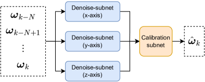
Figure 1: The overall network architecture of TinyGC-Net.

The overall network architecture is depicted in Figure XX, where $\boldsymbol{\omega}_{k}$ is the voltage reading of tri-axis gyroscope at timestamp $k$, $N$ is the length of local window, $\hat{\boldsymbol{\omega}}_{k}$ is the denoised and calibrated angular velocity in the unit of $rad/s$ at timestamp $k$.

3.1 Denoise Subnet

Through approximation, we assume that the three-axis measurement process of the gyroscope is independent of each other, allowing us to individually apply noise reduction processing to the measurement data of each axis.

Then, we define the denoise subnet structure which infers the denoised gyroscope’s measurements as

$$\hat{\omega}_{i,k}^{\prime}=f\left(\omega_{i,k-N+1},\cdots,\omega_{i,k}\right)$$ (4)

where the subscript $i$ indicates the $i$-axis of the gyroscope ($i=x,y,z$); $N$ is the length of the local window; $\omega_{i,k}$ is the voltage reading of gyroscope’s $i$-axis at timestamp $k$; $f(\cdot)$ is the mapping defined by the neural network; $\hat{\omega}_{i,k}^{\prime}$ is the denoised data.

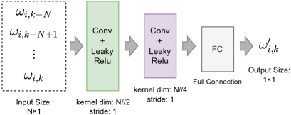
Figure 2: Denoise Subnet

The denoise subnet consists of three convolutional layers and three LeakyReLU layers, whose configurations are given in Figure XX. Essentially, we leverage the denoise subnet that infer a denoised data based on a local window of $N$ previous voltage readings of gyroscope’s $i-$axis. Since there is no coupling parameters between the three axis of gyroscope, the denoise subnet only requires hundreds of parameters totally by denoising the measurement for each axis individually.

3.2 Calibration Subnet

The calibration subnet is constructed as the figure XX. Essentially, the convolutional and concatenation operations within the dashed box in Figure XX are equivalent to Equation XX, both encompassing 12 parameters to be estimated, which we designate as linear basic network (LBN).

To accurately model the nonlinear components of the gyroscope measurement model, we employ the PReLU activation function [3] to connect two LBN modules, drawing inspiration from the structure of residual networks to facilitate faster convergence during training.

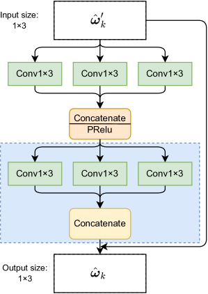
Figure 3: Calibration Subnet

remark 1:

Due to the continuous advancements in MEMS process technology, most manufacturers’ MEMS gyroscopes exhibit nonlinearity within a range of 0.01% in terms of angular rate measurement. On the other hand, according to our experimental observations, the cascading of multiple sub-networks can hardly bring enhanced calibration accuracy. Therefore, in the subsequent experiments detailed below, we only incorporate one LBN into TinyGC-Net.

3.3 Loss Function

Defining a proper loss function plays a critical role in training the calibration parameters involved in the neural network. Given that it is difficult and costly to obtain the ground truth values for every moment, we construct a simple loss function shown in Figure.xx, which only requires a few reference attitude information over a period of sampling time, and it is also convenient for the real scenarios without motion capture system.

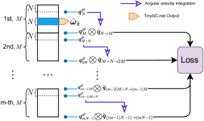
Figure 4: Loss function

In Figure.4, the quaternion $\boldsymbol{q}_{N}^{gt}$ represents the ground truth of the attitude angle at timestamp $N$; $\hat{\boldsymbol{q}}_{N\to M}$ represents the estimated attitude angle based on the equation (XX) from timestamp $N$ to $M$; the symbol $\bigotimes$ represents the difference between two quaternions, and we define it as follows in this paper:

$$\boldsymbol{q_{a}}\otimes\boldsymbol{q_{b}}=\sqrt{d{q}_{w}^{2}+d{q}_{x}^{2}+d{q}_{y}^{2}+d{q}_{z}^{2}}$$

where $\boldsymbol{q}_{a}=\left(q_{a,w},q_{a,x},q_{a,y},q_{a,z}\right)$ and $\boldsymbol{q}_{b}=\left(q_{b,w},q_{b,x},q_{b,y},q_{b,z}\right)$ are two distinct quaternion; $q_{a,w}$ and $q_{b,w}$ are the scalar parts; $\left(q_{a,x},q_{a,y},q_{a,z}\right)$ and $\left(q_{b,x},q_{b,y},q_{b,z}\right)$ are the vector parts; and

$$dq_{s}=q_{a,s}-q_{b,s},s=w,x,y,z.$$

As illustrated in Figure 5, the sequences of gyroscope measurements, each with a length of $mM$, will be segmented into $m$ equal parts, each part being $M$ in length. Within each segment, TinyGC-Net employs a local sliding window mechanism to analyze the raw gyroscope measurement data within the local window of length $N$ and perform local noise reduction and calibration. This localized processing aids in capturing short-term dynamic changes in the gyroscope measurement data and suppresses high-frequency noise within the measurements.

For the $j$-th gyroscope measurement sequence of length $M$, the cost function can be represented as follows:

$$\mathcal{L}_{j}=\boldsymbol{q}_{jM}^{gt}\otimes\hat{\boldsymbol{q}}_{(j-1)M+N\to{jM}}$$ (5)

4 Observability Analysis

5 Experiments

To verify the validity of the TGC-Net, we carry out the experiments based on the public datasets and real-world scenarios in this section.

5.1 Experiments on public datasets

5.1.1 Data Sources and Training Details

The european robotics challenge (EuRoC) microair vehicle (MAV) dataset [4] is a visual inertial dataset, which contains IMU sequences at 200Hz from an ADIS16448 MEMS IMU sensor, and an external Vicon system is used to provide the pose ground truth. For ease of comparison with previous work, we use MH{01, 03, 05}, V1{02} and V2{01, 03} in EuRoC dataset for training while the rest are used for testing.

The network of this paper is implemented using PyTorch, and we training it using a i7-13790F CPU. The training process use the AdamW optimizer [5], and set the learning rate as 0.01.

In the training process, the whole network only requires $90$ parameters to be trained, which is extremely fewer than other calibration model based on deep learning. And the 2000 epochs of training take about 10 min ($N=50$, $M=200$).

5.1.2 Metrics Definitions

We utilize absolute orientation error (AOE) [6] to quantitatively assess the performance of the proposed method. The AOE computes the mean square error between the ground truth and the estimated orientation, which can be described as follows

$$\mathrm{AOE}=\sqrt{\sum_{n=1}^{L}\frac{1}{L}\left\|\log\left(\mathbf{R}_{n}^{T}\hat{\mathbf{R}}_{n}\right)\right\|_{2}^{2}}$$ (6)

where $L$ represents the sequence length; $log(\cdot)$ is the $SO(3)$ logarithm map.

5.1.3 Compared Methods

We compare two existing methods based on deep learning for calibrating gyroscopes:

(1) Raw: uncalibrated gyroscope measurement. For the majority of low-cost MEMS gyroscopes, users are typically provided with a scale factor from the chip’s datasheet to convert the gyroscope’s voltage measurements into corresponding angular velocities, without accounting for the effects of misalignment and non-orthogonality on the measurement values;

(2) DIG[7]: the heavyweight network using convolutions to denoise the gyroscope noise;

(3) OriNet[8]: the network based on long short-term memory (LSTM);

(4) TinyGC: our proposed method described in Section XXX.

5.1.4 Experimental result

The experimental results are given in Table 1. And figure 5 and figure 6 illustrates roll, pitch, and yaw estimates for the sequence V2_02_medium and MH_04_difficult.

Table 1: Absolute Orientation Error (AOE) in terms of 3D Orientation in degree on the test sequences.

	raw	DIG	OriNet	TinyGC ($M$=200, Full)	TinyGC ($M$=600, Full)	TinyGC ($M$=200, 30s)	TinyGC ($M$=600, 30s)
MH_02_easy	146	1.39	5.75	4.88	5.18	1.11	1.47
MH_04_difficult	130	1.40	8.85	3.64	4.96	0.98	1.79 j
V1_01_easy	71.3	1.13	6.36	4.41	6.06	2.58	2.84
V1_03_difficult	119	2.70	14.70	2.49	8.11	1.24	1.36
V2_02_medium	117	3.85	11.70	5.38	5.03	2.10	4.49
average	125	2.10	9.46	4.17	5.87	1.60	2.39
parameter count	-	77052	-	180	180	180	180
training platform	-	GPU	GPU	GPU	GPU	GPU	GPU
deployment platform	-	GPU	GPU	CPU&MCU	CPU&MCU	CPU&MCU	CPU&MCU

• OriNet uses LSTM network, and its model parameters are more complex and take longer time than DIG.

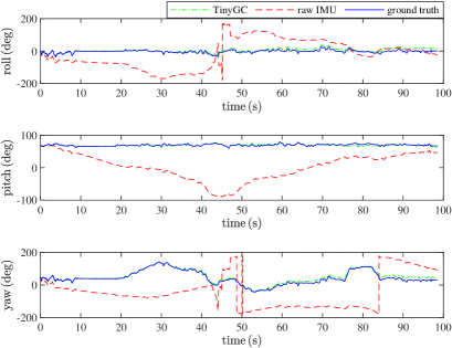
Figure 5: Orientation estimates on the test sequence V2_02_medium

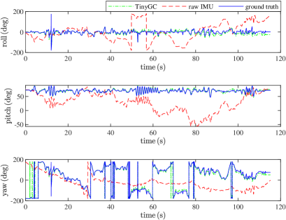
Figure 6: Orientation estimates on the test sequence MH_04_difficult

According to the experiment results, we note that:

(1) TinyGC requires minimal parameters, and is the only scheme among all the solutions that can be easily implemented on MCUs with limited computational resource.

(2) TinyGC outperforms OriNet by about $1.5$ times with more concise network structure.

(3) DIG achieved the highest accuracy, while both training and operation require the use of a GPU. Besides, OriNet uses LSTM network, its model parameters are more complex and take longer time compared with DIG.

(4) The uncalibrated gyroscope measurements are unreliable, and the orientation angles derived from the integration of raw gyroscope measurements are prone to rapid drift.

(5) The denoising effect of the denoise subnet is evident, with the high-frequency noise in the gyroscope measurements being effectively suppressed.

5.1.5 Remark

We provide a few more remarks based on the process of our research:

(1) Essentially, almost all learning-based gyroscope calibration methods introduce accelerometer measurement information to constrain the time-varying offset of the gyroscopes, which can effectively enhance the estimation accuracy of the orientation angles. However, this treatment necessitates an increased number of model parameters to establish the relationship between accelerometer and gyroscope measurements, and requires regularization techniques such as weight decay and dropout during training to mitigate the issue of overfitting.

(2) The calibration subnet is a linear model. We have attempted to employ a multi-layer network with the introduction of activation functions to construct the calibration subnet with non-linear characteristics, but this approach yielded negligible improvements in the estimation accuracy of the orientation angles. On the other hand, the non-linearity of the gyroscope is only 0.01% of its dynamic range according to the datasheet of the ADIS16488 (used in the EuRoC dataset). Consequently, the Calibration Subnet comprises only three convolutional layers, and its mathematical model is equivalent to Equation (2).

(3) To reduce the number of parameters, the denoise subnet independently performs noise reduction on the X, Y, and Z-axis measurements of the gyroscope. This not only effectively suppresses high-frequency noise but also introduces less latency compared to classical Finite Impulse Response (FIR) and Infinite Impulse Response (IIR) filters.

(4) It is important to note that some of the datasets exhibit very dynamic motions, which are known to deteriotate the measurement accuracy of the laser tracking device [4], which can not guarantee the precision of the pose ground truth, and leads to the relatively large training loss and validation loss during training.

Reference

References

- [1] Chua L O and Roska T 1993 IEEE Transactions on Circuits and Systems I: Fundamental Theory and Applications 40 147–156
- [2] Ru X, Gu N, Shang H and Zhang H 2022 Micromachines 13 879
- [3] Ding B, Qian H and Zhou J 2018 Activation functions and their characteristics in deep neural networks 2018 Chinese control and decision conference (CCDC) (IEEE) pp 1836–1841
- [4] Burri M, Nikolic J, Gohl P, Schneider T, Rehder J, Omari S, Achtelik M W and Siegwart R 2016 The International Journal of Robotics Research 35 1157–1163
- [5] Loshchilov I and Hutter F 2017 arXiv preprint arXiv:1711.05101
- [6] Grupp M 2017 evo: Python package for the evaluation of odometry and slam. https://github.com/MichaelGrupp/evo
- [7] Brossard M, Bonnabel S and Barrau A 2020 IEEE Robotics and Automation Letters 5 4796–4803
- [8] Esfahani M A, Wang H, Wu K and Yuan S 2019 IEEE Robotics and Automation Letters 5 399–406