Comparative analysis of diverse methodologies for portfolio optimization leveraging quantum annealing techniques

Abstract

Portfolio optimization (PO) is extensively employed in financial services to assist in achieving investment objectives. By providing an optimal asset allocation, PO effectively balances the risk and returns associated with investments. However, it is important to note that as the number of involved assets and constraints increases, the portfolio optimization problem can become increasingly difficult to solve, falling into the category of NP-hard problems. In such scenarios, classical algorithms, such as the Monte Carlo method, exhibit limitations in addressing this challenge when the number of stocks in the portfolio grows. Quantum annealing algorithm holds promise for solving complex portfolio optimization problems in the NISQ era. Many studies have demonstrated the advantages of various quantum annealing algorithm variations over the standard quantum annealing approach. In this work, we conduct a numerical investigation of randomly generated unconstrained single-period discrete mean-variance portfolio optimization instances. We explore the application of a variety of unconventional quantum annealing algorithms, employing both forward annealing and reverse annealing schedules. By comparing the time-to-solution(TTS) and success probabilities of diverse approaches, we show that certain methods exhibit advantages in enhancing the success probability when utilizing conventional forward annealing schedules. Furthermore, we find that the implementation of reverse annealing schedules can significantly improve the performance of select unconventional quantum annealing algorithms.

I Introduction

The portfolio optimization problem is a well-known finance challenge that aims to maximize the possible returns while minimizing risk. The objective of solving this problem is to determine an optimal asset allocation that meets the specified requirements. However, the complexity of the portfolio can escalate to NP-hard levels as the number of involved assets and constraints increases [1, 2]. Classical algorithms, including the commonly used Monte-Carlo algorithm, may fail to provide efficient solutions due to the computational complexity associated with the portfolio optimization problem.

Quantum computing has benefits in solving certain hard problems where classical algorithms fail [3, 4, 5, 6, 7, 8, 9, 10, 11, 12, 13, 14, 15, 16, 17, 18]. Its applicability extends to many disciplines, including artificial intelligence [19, 20, 21, 22, 23, 24, 25, 26], finance [27, 28, 29], the optimization of complex systems [30, 31, 32], and drug discovery [33, 34, 35, 36]. The fundamental operating units in quantum computers are essentially different from their classical counterparts. Quantum computing leverages the phenomenon of quantum entanglement, which enables extensive parallel processing by allowing the simultaneous operation of multiple states. Additionally, quantum superposition provides a vast storage space compared to classical bits. These unique characteristics of quantum computing offer the potential for exponential advancements in computational power and storage capabilities, surpassing the limitations of classical computing systems. The gate-model quantum computing, which employs quantum logical gates for information processing, is the most extensively studied quantum computing model and has been proven to be universal computation [37]. However, the fragility of qubits poses a significant challenge in scaling up quantum gate model computers in practice applications. Quantum error correction and fault tolerance techniques that are required in the implementation of quantum gate model computer can lead to large resource overhead costs [38, 39, 40, 41, 42, 43, 44]. As a result, current quantum gate model computers are limited to a few hundred qubits [45]. As an alternative to the quantum gate model, quantum annealing is extensively used in solving optimization problems. The scale of quantum annealing hardware can reach thousands of qubits [46, 47]. The high scalability of quantum annealer enables more practical implementations of quantum computation.

The most commonly used techniques in portfolio optimization problems, such as mean-variance model [48], Value-at-Risk [49, 50], and Conditional Value-at-Risk [51], have been extensively studied with classical methodologies, including statistical and artificial intelligence approaches [52, 53, 54, 55, 56, 57]. The investigations on portfolio optimization utilizing quantum computing have been conducted with gate-based models, employing techniques such as the quantum approximate optimization algorithm (QAOA) [58, 59, 60, 61], the variational quantum eigensolver (VQE) [59, 62, 63], the quantum algorithm for linear systems of equations(HHL) [64, 61], and the quantum annealing algorithm [65, 66, 67, 68, 16, 69, 70, 71, 72, 27, 63, 73, 74, 75]. Portfolio optimization problems involving diverse financial assets can lead to an exponential number of variables. Gate-based models are constrained in addressing the challenges due to the hardware limitations. Consequently, quantum algorithms employed for portfolio optimization problems predominantly rely on quantum annealing in the NISQ era, even when considering the limited connectivity of current quantum annealing hardware.

In the context of quantum annealing, a portfolio optimization problem can be encoded as a problem Hamiltonian. The system evolves from the ground state of an easily prepared initial Hamiltonian to the ground state of the problem Hamiltonian. According to the adiabatic theorem, if the system’s evolution is sufficiently slow, the final ground state attained by the system will encode the solution to the optimization problem. Various adaptations of QA have demonstrated advantages over the conventional QA [76, 77, 78, 79, 80, 81, 82, 83, 84, 85, 86]. The standard QA involves a stoquastic Hamiltonian, wherein the off-diagonal elements are real and non-positive. A stoquastic Hamiltonian that avoids “sign problem” can be efficiently simulated using classical algorithms like Quantum Monte Carlo(QMC). Thus, it’s valuable to explore some variants of standard QA that employ non-stoquastic Hamiltonians. Additionally, the reverse annealing protocol has been proven to provide quantum advantages [87, 68, 88]. Therefore, it is also worthwhile to explore variants of QA that incorporate the reverse annealing schedule.

Recent research lacks a comprehensive study that compares different variants of QA in the domain of solving portfolio optimization problems. We believe that such a study has the potential to provide valuable guidance for the experimental implementation of QA. To address this research gap, we propose conducting an in-depth investigation into the portfolio optimization problem utilizing a carefully selected ensemble of unconventional QA algorithms. Additionally, we intend to conduct a comparative analysis of the performance of each algorithm, utilizing both forward annealing and reverse annealing.

The paper is structured as follow: in Section II we introduce the formulation of the portfolio optimization problem and the recent developments. Section III describes different promising variants of QA like adding transverse couplers to standard QA, inhomogeneous driving QA, RFQA and CDQA. Section IV introduces the reverse annealing schedule. And section V is devoted to the numerical results, we compare the time-to-solution and success probability of each algorithm, utilizing both forward annealing and reverse annealing. In Section VI we conclude with a discussion and considerations for future work.

II Portfolio optimization formulation

Portfolio optimization is a challenging problem in finance and management. Its objective is to find a balance between risk and return. For instance, the general formulation of Markowitz’s mean-variance model can be expressed as follows [59]:

$$\max_{x}\left\{\sum_{i}^{n}\mu_{i}x_{i}-q\sum_{i,j}^{n}\sigma_{ij}x_{i}x_{j}-\lambda\left(B-\sum_{i}^{n}x_{i}\right)^{2}\right\},$$ (1)

the given formulation in Markowitz’s mean-variance model is a binary constrained mean-variance model. This model addresses the binary portfolio optimization problem, where the variables are limited to values of 0 or 1, $\mu_{i}$ is the expected return of assets, $\sigma_{ij}$ is the risk of assets, and $B$ is the full budget.

The formulation of a particular portfolio optimization depends on the given market conditions. To adapt a portfolio optimization problem for quantum annealing, it is necessary to transform the formulation into a Quadratic Unconstrained Binary Optimization (QUBO) problem through various conversions, such as binary, unary, or sequential encoding. [89, 65]. The problem is encoded into a problem Hamiltonian $H_{P}$, which is defined by pauli matrices

$$H_{P}\ =\ \sum_{i}^{n}h_{i}\sigma_{i}^{z}\ +\ \ \sum_{i,j}^{n}J_{ij}\sigma_{i}^{z}\sigma_{j}^{z}\ +\ C,$$ (2)

where $h_{i}$ is the qubit biases, $J_{ij}$ is the coupling strength between qubit $i$ and $j$, $C$ is a constant generated from the transformation and can be omitted in the following expressions. Unlike the transverse field ising model(TFIM) [90], which considers the nearest neighbour interactions, the Ising spin-glass model derived from the portfolio optimization problem encompasses all-to-all connections. Current quantum annealer such as the D-Wave machine has limited connectivity due to the QPU topology. However, as the hardware technology advances, we believe it is worthwhile simulating the behavior of promising quantum annealing algorithms for future implementation.

Quantum-based algorithms have demonstrated their efficacy in enhancing portfolio optimization outcomes, such as the works using gate-model Quantum computing in [59, 64, 60, 91, 92, 62, 61, 93, 94] and the ones using Quantum annealing algorithms in [65, 67, 68, 69, 70, 70, 95, 27, 73, 74, 75, 96]. Despite the limited connectivity of quantum annealers, they provide more accessible stable qubits than gate-model quantum computer in the NISQ era. Consequently, our focus in this study will be on evaluating the performance of different quantum annealing algorithms. To make a comprehensive comparison of QA algorithms for solving the portfolio optimization problem, we transform the portfolio optimization model into an ising model and simulate the annealing process under the guidance of time dependent Schrodinger equation. Various adaptations of QA algorithms are studied and compared to provide guidance for their implementation on real quantum hardware. Furthermore, the reverse annealing of each algorithm is investigated and introduced in the following sections.

III Unconventional QA methods

The formulation of standard quantum annealing is as follows,

$$H(t)\ =\ A(t)H_{0}+B(t)H_{P},$$ (3)

the initial Hamiltonian $H_{0}$ and problem Hamiltonian $H_{P}$ are not commute with each other, the annealing parameters $A(t)$ and $B(t)$ follows the routine that $A(t)\gg B(t)$ at the beginning and $B(t)\gg A(t)$ at the end. In the forward annealing routine, $A(t)$ monotonically decreases while $B(t)$ monotonically increases. The initial Hamiltonian, conventionally chosen as $H_{0}=-\sum_{i=1}^{n}h\sigma_{i}^{x}$, has an easily prepared ground state. Its ground state $\ket{+}^{\bigotimes n}$ is the uniform superposition state, where $\ket{+}=\ \frac{1}{\sqrt{2}}(\ket{0}+\ket{1})$. The problem Hamiltonian is usually prepared with pauli-z matrices so that $H_{P}$ doesn’t commute with $H_{0}$. The ground state of $H_{P}$ encodes the solution to the computational optimization problem.

In standard quantum annealing, the total Hamiltonian interpolates between the initial Hamiltonian and problem Hamiltonian under slowly adiabatic evolution, the system will stay on the instantaneous ground state according to the adiabatic theorem. The total annealing time is proportion to the inverse of squared minimum energy gap $t_{f}\propto\Delta_{min}^{2}$ , the probability of staying on the ground state can be approximated as $P_{t_{f}}=\ 1-e^{-\alpha t_{f}}$ [97]. For problems that go through first order transition, the evolution time required to reach a reasonable success probability will grow exponentially with the system size. However, it’s not ideal to solving realistic problems with an exponentially long evolution time. Some techniques that can provide speedup on short time evolution emerges for practical use requirements. We introduce them in the following subsections.

III.1 Coupler QA

In the work of [76, 77, 78, 79], adding a 2-body transverse coupler is proven to boost the traditional quantum annealing algorithm in solving some classes of problem. The formulation of the total Hamiltonian is given as:

$$H(t)\ =(1-s(t))H_{0}+s(t)H_{P}+(1-s(t))s(t)H_{I}.$$ (4)

The coupler term can be ferromagnetic coupler $H_{I}^{F}$, antiferromagnetic coupler $H_{I}^{A}$, or a mixed coupler $H_{I}^{M}$. They are defined as follows

$$H_{I}^{F}=-\sum_{<i,j>}^{N}{\sigma_{i}^{x}\sigma_{j}^{x}}$$ (5)

$$H_{I}^{A}=+\sum_{<i,j>}^{N}{\sigma_{i}^{x}\sigma_{j}^{x}}$$

$$H_{I}^{M}=\sum_{<i,j>}^{N}{r_{ij}\sigma_{i}^{x}\sigma_{j}^{x}},$$

where $r_{ij}$ can be a random number chosen from $\{-1,1\}$. The coupler term disappears at the beginning and the end of the annealing process, ferromagnetic coupler keeps the stoquastic of the tranditional QA, anti-ferromagnetic and mixed coupler forms non-stoquastic Hamiltonians. The work in [78] shows that adding transverse coupler outperforms the tranditional QA. Studies on constructing non-stoquastic Hamiltonians with $H_{I}^{F}$ or $H_{I}^{M}$ have shown the enhanced capabilities of the transverse couplers [98, 76, 77], they can help to avoid the first order phase transition in some certain systems.

III.2 Inhomogeneous driving QA

In addition to adding transverse coupler to the transverse driving field, an inhomogeneous driving field can weaken the effect of phase transition and lead to a better performance [80, 81] compared with traditional QA, the formulation is given by

$$H(t)\ =H_{V}(t)+s(t)H_{P},$$ (6)

unlike the uniform transverse field in standard QA, the inhomogeneous driving Hamiltonian $H_{V}(t)$ can be defined as

$$H_{V}(t)=-\sum_{i=1}^{N(1-\tau)}\sigma_{i}^{x},$$ (7)

where $\tau$ is another annealing controller similar to $s(t)$ that starts from 0 and ends up with 1 so that the transverse field on each qubit will be turned off starting from site $N$ to site 1. The $H_{V}(t)$ term can also be represented by a continuous function $\Gamma_{i}(t)$ as follow

$$H_{V}(t)=-\sum_{i=1}^{N}\Gamma_{i}(s)\sigma_{i}^{x},$$ (8)

the continuous filed amplitude $\Gamma_{i}(t)$ is applied to each qubit and will be reduced sequentially. The definition of $\Gamma_{i}(t)$ given in  [81] is

$$\begin{split}&\Gamma_{i}(s)=\begin{cases}1&\text{if $s<s_{i}$}\\ N(1-s^{r})+(1-i)&\text{if $s_{i}\leq s\leq s_{i-1}$}\\ 0&\text{if $s_{i-1}<s$}\\ \end{cases}\end{split}$$ (9)

where $s_{i}=(1-\frac{i}{N})^{\frac{1}{r}}$ and $r=0.5$ is chosen in our work. Such a continuous function can be reduced to Eq.7 as $N\to\infty$ and will circumvent the sudden change in Hamiltonian.

Experimental implementation and analytical studies of inhomogeneous driving QA have shown its ability to enhance the success probability for some specific instances [99, 100]

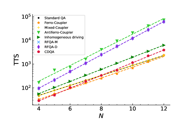
Figure 1: Shown is the time required to identify the true ground state in randomly generated instances using various unconventional QA methods with a forward annealing schedule. The runtime is $t_{f}=1$. The data points corresponding to the standard QA method are depicted as black dots, while the black solid line represents the best-fit curve for the data. Other markers and dashed lines are used to represent other methods for comparison purpose. The presented results are the average of 500 randomly generated instances.

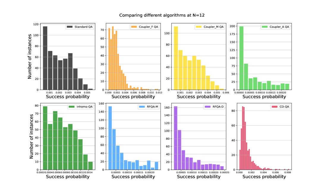
Figure 2: A comparison of the ground state success probability of different algorithms employing the forward annealing schedule at N=12. For each algorithm, 500 random instances were generated.

III.3 RF-QA

Traditional QA finds the ground state by adiabatically evolve the system to avoid the diabatic transitions nearby the energy gap. RFQA method is a new variant of QA that enhance the probability of finding ground state by taking advantage of diabatic transitions. RFQA modifies the conventional uniform transverse field into oscillating field and leave the problem Hamiltonian unchanged, the modified field can be either transverse field with oscillating magnitude or a uniform field with oscillating direction in x-y plane. RFQA method can be implemented in current hardware by making some modifications to the control circuitry [82].

The RFQA field with oscillating magnitude is refered to as $RFQA-M$, $M$ stands for magnitude. The formulation of the driving field in RFQA-M is denoted by

$$H_{M}=-\sum_{i}^{N}{(1+\bar{\alpha_{i}}sin(2\pi f_{i}t))\sigma_{i}^{x}},$$ (10)

in which $\bar{\alpha_{i}}$ represents the amplitude of the field, and the frequency $f_{i}$ is randomly chosen and applied to each spin $i$, the low frequency oscillating field induces multi-photon resonances during the annealing process, the proliferating multi-photon resonances can rapidly mix the ground state and first excited states at the adjacent of the minimum gap, and provides a polynomial speedup over the traditional quantum annealing algorithm theoretically [82].

The oscillating field can also be realized by oscillating the direction in x-y plan, which we refer to $RFQA-D$ method, $D$ represents direction here, the field in RFQA-D is denoted by

$$H_{D}=-\sum_{i}^{N}[cos(\bar{\alpha_{i}}isin(2\pi f_{i}t))\sigma_{i}^{x}+sin(\bar{\alpha_{i}}isin(2\pi f_{i}t))\sigma_{i}^{y}].$$ (11)

The Hamiltonian in RFQA method is defined as follow

$$H(t)\ =(1-s(t))H_{M/D}+s(t)H_{P}.$$ (12)

The advantages of RFQA have been shown in [83], which shows a polynomial quantum speedup of RFQA in solving an artificial problem with competing ground states.

Algorithm	Scaling exponent
Standard QA	0.70
Ferro Coupler QA	0.75
Mixed Coupler QA	0.70
Anti-ferro Coupler QA	1.10
Inhomogeneous QA	0.85
$RFQA_{M}$	1.17
$RFQA_{D}$	1.16
CD-QA	0.89

Table 1: The scaling exponents for each method employ the forward annealing schedule. The $TTS(N)$ of each approach is modeled by fitting it into the $2^{\beta+\alpha N}$ function. We present the exponential scaling coefficient “$\alpha$” for each method in the table for comparison purposes.

III.4 CD-QA

In standard QA, the ground state of $H_{P}$ can be found with high probability after annealing time that relates to the minimum energy gap. In some problems with exponentially small energy gap, the required annealing time can be extremely long. To make quantum annealing more practical to use, the idea of suppressing nonadiabatic transition during short time evolution was proposed [84, 85, 86], the non-adiabatic technique is named as counter-diabatic quantum annealing (CD-QA). The effectiveness of CD-QA has been proven in the works [101, 102, 103, 104, 105, 106, 107, 108, 109, 110, 111, 112, 27, 113, 114, 115, 116, 117]

The idea of CD-QA is taking advantage of the Adiabatic Gauge Potential(AGP) to suppress the non-adiabatic transition in quantum annealing. By transforming the original Hamiltonian $H_{origin}(t)$ in a specific rotating frame that consists of a static effective Hamiltonian and an adiabatic gauge potential related Hamiltonian which contribute to the excitations between eigenstates, we can add a Hamiltonian to $H_{origin}(t)$ so that the quantum state keeps adiabaticity and evolves to the ground state in a shorter time.

We can formulate the total Hamiltonian in CD-QA as follow(Appendix A):

$$H(t)\ =H_{origin}(t)\ +\ H_{CD},$$ (13)

the counter-diabatic driving term can be chosen as:

$$H_{CD}=\dot{\lambda}\sum_{i}^{N}{\alpha_{i}\left(t\right)\sigma_{i}^{y}}.$$ (14)

The annealing schedule $\lambda(t)$ can be chosen as $\lambda(t)={sin}^{2}[{\frac{\pi}{2}sin}^{2}(\frac{\pi t}{2T})]$ so that the CD driving term vanishes at $t=0$ and $t=t_{f}$. And $\alpha_{i}(t)$ specifically for the ising model is derived in Appendix A.

Ideally, one can evolve the system in a short time without excitations between the eigenstates. This concept is widely used in many fields such as quantum physics, stochastic physics.

IV Reverse annealing

Algorithm	Scaling exponent
Standard QA	1.00
Reverse Standard QA	0.34
Reverse Ferro Coupler QA	0.35
Reverse Mixed Coupler QA	0.34
Reverse Anti-ferro Coupler QA	0.35
Reverse $RFQA_{M}$	0.09
Reverse $RFQA_{D}$	0.09

Table 2: The scaling exponents for certain methods employ the reverse annealing schedule and the standard QA employ the forward annealing schedule. The $TTS(N)$ of each approach is modeled by fitting it into the $2^{\beta+\alpha N}$ function. We present the exponential scaling coefficient “$\alpha$” for each method in the table for comparison purposes.

In conventional forward quantum annealing, the transverse field is initially activated and subsequently reduced as the annealing process progresses, allowing the system to explore the entirety of the solution space. For most practical NP-hard problems that are described by the Ising model, the conventional routine can be doomed by exponentially small gaps in the spin-glass phase [118]. Reverse annealing that takes advantage of partial knowledge on the solution space can offer the potential for more efficient exploration of the true solution. The idea of reverse annealing is starting from a candidate initial state that is obtained by other methods, such as classical algorithms. The transverse field strength is initialized at $s=1$ and subsequently decreased to a finite value, followed by a pause. Finally, it is ramped up again to $s=1$. The system starts the exploration of the solution space from a candidate state nearby the solution in such a reverse annealing routine, thereby enhancing the efficiency of the search process. The advantages of reverse annealing are revealed in some works [119, 87, 120]. Reverse annealing can be described by the follow formulation

$$H(t)\ =\ sH_{p}+(1-s)H_{0},$$ (15)

where $H_{p}$ and $H_{0}$ represent the problem and initial Hamiltonians as in conventional forward annealing QA. However, the annealing parameter $s$ differs from that used in conventional forward annealing QA.

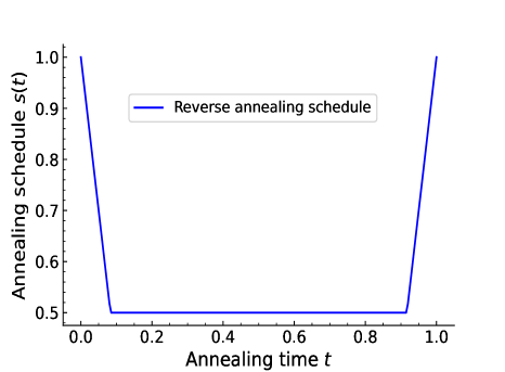
Figure 3: The reverse annealing schedule $s(t)$ initiates at 1, where the problem Hamiltonian dominates. Following this, $s(t)$ is gradually reduced to 0.5 and remains at this value for a relatively long time before being increased back to 1.

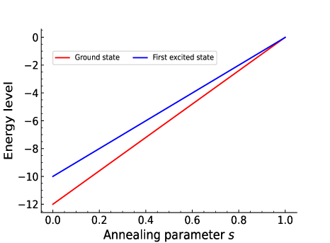
Figure 4: The energy levels of the hard instance at $N=12$. The ground state is represented by the red solid line, while the first excited state is represented by the blue line. An avoided small energy gap appears near the end of the annealing schedule.

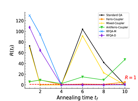
Figure 5: The advantages ration $R(t_{f})$ of the hard instance at $N=12$. The red dashed line represents $R=1$, indicating whether an algorithm achieves performance advantages with the help of reverse annealing schedule. The other solid lines correspond to the advantages ratio of each algorithm.

The reverse annealing schedule in this work is illustrated in FIG. 3, the annealing parameter $s$ starts at 1, ramps down to $s=0.5$ and pause at $s=0.5$ for a long time, and then ramp up to $s=1$.

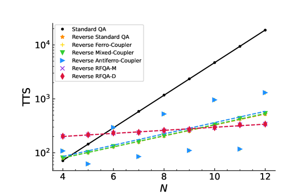
Figure 6: Shown is the time required to find the true ground state in randomly generated instances using various unconventional QA methods with a reverse annealing schedule. The runtime is $t_{f}=1$. The data of the standard QA method are denoted by black dots, and the black solid line represents the best-fit curve of the data. Other markers and dashed lines are used to represent the results of other methods for comparison purpose. The results presented are averaged over 500 randomly generated instances.

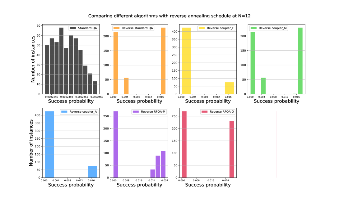
Figure 7: A comparison of the ground state success probability between certain methods that use the reverse annealing schedule and the standard QA that employs the forward annealing schedule at N=12. For each algorithm, 500 random instances were generated.

V Results and Discussion

In this section, we present and discuss the quantitative results obtained from a performance comparison of alternative QA approaches, employing both forward and reverse annealing schedules. These findings aims to provide guidance on the experimental implementation of these approaches.

In the study employing the forward annealing schedule, we generate 500 random instances for the unconstrained single-period discrete portfolio optimization problem. For each method, we determine the success probability within an annealing time $t_{f}=1$. The system size ranges from $N=4$ to $N=12$. In addition to the success probability, we compute another performance metric called time-to-solution(TTS) to evaluate the algorithms’ performance. TTS calculates the time needed to obtain a solution with 99% success probability:

$$TTS\propto t_{f}\frac{\ln(1-0.99)}{\ln(1-p(t_{f}))}.$$ (16)

As illustrated in FIG. 1, the randomly generated instances for portfolio optimization demonstrate exponential complexity, as the time-to-solution grows exponentially with system size $N$. We see that the unconventional QA algorithms do not exhibit obvious advantages over standard QA approach. To make a more intuitive comparison, we fit the $TTS(N)$ of each method with an exponential function $2^{\beta+\alpha N}$ and list the extracted exponent $\alpha$ in TABLE I. It is evident that only the mixed coupler QA approach is comparable to the standard QA. However, this doesn’t imply that the unconventional QA algorithms lack value in addressing portfolio optimization problems. In FIG. 2, we present the success probability of the 500 instances and demonstrate that methods such as the Ferromagnetic coupler QA, Mixed coupler QA and CDQA can enhance the success probability in certain cases.

In the study employing the reverse annealing schedule, we find one hard instance that contains a local minimum and we designate this local minimum as the initial state for the reverse annealing schedule. The energy gap of the hard instance is depicted in FIG. 4, revealing the presence of an avoided energy gap between the first excited state and the ground state towards the end of the annealing schedule. This avoided gap is extremely small, thereby inducing diabatic transitions between the two competing states. To show how the advantages provided by reverse annealing changes with annealing time, we conducted a comparative analysis of the success probability for some algorithms annealed using both forward and reverse annealing schedules. This analysis was performed over a range of short annealing times, specifically from $t_{f}=1$ to $t_{f}=10$, as depicted in FIG. 5. We define the success probability of each algorithm as $P_{f}(t_{f})$ for the forward annealing schedule and $P_{r}(t_{f})$ for the reverse annealing schedules. To quantify the advantages of the reverse annealing schedule in each algorithm, we denote the advantage as the ratio

$$R(t_{f})=\frac{P_{r}(t_{f})}{P_{f}(t_{f})}.$$ (17)

The advantages ratio for each algorithm is denoted as $R_{S}(t_{f})$, $R_{F}(t_{f})$, $R_{M}(t_{f})$, $R_{A}(t_{f})$, $R_{RM}(t_{f})$, $R_{RD}(t_{f})$, where “S”, “F”, “M”, “A”, “RM”, and “RD” represent standard QA, Ferro Coupler QA, Mixed Coupler QA, Anti-ferro Coupler QA, RFQA-M, and RFQA-D, respectively. For example, $R_{S}(t_{f})$ is the ratio of the standard QA using the reverse annealing schedule to the standard QA using the forward annealing schedule. As shown in FIG. 5, the dashed red line at $R=1$ represents the scenario where the reverse annealing schedule does not exhibit any advantages. It’s evident that all the methods demonstrate significant advantages in most cases. Reverse annealing that starts from a known possible solution provides obvious help in enhancing the success probability of finding the true ground state. Furthermore, we studied how the quantum advantages provided by reverse annealing changes with system size from $N=4$ to $N=12$. The time-to-solution (TTS) comparison between algorithms employing the reverse annealing schedule and the standard QA approach using the forward annealing schedule is depicted in FIG. 6. Additionally, the TTS scaling exponent for each algorithm is listed in TABLE II. The findings presented in FIG. 6 and TABLE II indicate that all methods, with the assistance of reverse annealing, exhibit promising quantum advantages in solving challenging portfolio optimization problem sets when compared to the standard QA approach utilizing the forward annealing schedule. Specifically for the system size at $N=12$, we conduct a comparison of the success probability between the standard QA approach using the forward annealing and other methods employing the reverse annealing schedule, as depicted in FIG. 7. 500 random instances are generated for the purpose of comparison. Notably, the methods utilizing the reverse annealing schedule exhibit significant improvements in the success probability for certain instances.

VI Conclusion

In this work, we investigated the portfolio optimization problem using different promising unconventional QA algorithms. We show that certain algorithms have the capability to improve the success probability compared to the standard quantum annealing algorithm in specific cases. Furthermore, we observed that the advantages can be further augmented with the help of the reverse annealing schedule.

In the context of the forward annealing schedule, we generated problem instances randomly and compared the time-to-solution exponent and success probability of each method. The simulation results reveal that while the unconventional QA methods may not exhibit obvious advantages in improving the averaged time-to-solution, certain methods such as coupler-QA and CD-QA demonstrate an enhanced success probability compared to the standard QA approach.

In the investigation with reverse annealing, we examined the behavior of standard QA, Coupler-QA and RFQA with the reverse annealing schedule. Specifically, we explored how the advantages ratio of reverse annealing changes with annealing time on a specific hard instances characterized by an extremely small avoided energy gap. FIG. 5 indicates that reverse annealing effectively enhances the success probability of standard QA, Coupler-QA and RFQA in most cases, particularly at short annealing times. The improvement in success probability is further illustrated in FIG. 7. Moreover, we compared the time-to-solution scaling of each methods using reverse annealing. The findings presented in FIG. 6 and TABLE II clearly indicate the significant quantum advantages provided by reverse annealing.

In conclusion, the utilization of unconventional QA methods has demonstrated the potential to enhance the success probability in certain cases. Moreover, the application of the reverse annealing schedule has significantly improved the performance of selected methods. We believe that the comprehensive quantitative assessment of time-to-solution and success probability for each method serves as a crucial step towards their experimental implementation in the NISQ era. It is worth noting that the portfolio optimization model employed in this study is the Markowitz portfolio model, where risk is estimated using the standard deviation. For future work, exploring alternative metrics such as the Sharpe ratio and CVaR could be considered.

Appendix A CD-QA Hamiltonian Derivation

To suppress the nonadiabatic transition, the adiabatic gauge potential (AGP) $A_{\lambda}$ is introduced into the Hamiltonian H in the lab frame and transform the Hamiltonian into a stationary effective Hamiltonian ${H^{\prime}}_{eff}$ in a rotating frame [121, 122]. For the state $\ket{\psi}$ in the lab frame, the corresponding state $\ket{\widetilde{\psi}}$ in the rotating frame becomes $\ket{\widetilde{\psi}}=\ U^{{\dagger}}(\lambda(t))\ket{\psi}$, $U$ is the unitary transformer between the frames and $\lambda$ is the parameter that controls the evolution of $H$. The evolution of the state in rotating frame is guided by the time dependent Schrodinger equation

$$i\hbar\frac{d\ket{\widetilde{\psi}}}{dt}=H_{eff}\ \ket{\widetilde{\psi}}=(U^{{\dagger}}HU-\ i\hbar\dot{\lambda}U^{{\dagger}}\partial_{\lambda}U)\ket{\widetilde{\psi}}.$$ (18)

The first term in the right-hand side is a diagonal term and only the second term contributes to the excitations between eigenstates. By adding the adiabatic gauge potential $A_{\lambda}=i\hbar\partial_{\lambda}UU^{{\dagger}}$ , the corresponding effective Hamiltonian becomes $U^{{\dagger}}HU$ and the state in the rotating frame becomes stationary state, the nonadiabatic transition is largely suppressed as a result.

The limitation of this approach is that the exact AGP is always consists of nonlocal terms, which is challenging to implement with the current quantum hardware. Thus, approximate methods for finding optimal CD driving protocols that can be easier to implement with local operations are proposed in [123]. In the ising model $H_{Ising}\ =\ \sum_{i=1}^{n}h_{i}\sigma_{i}^{z}\ +\ \ \sum_{<i,j>}^{n}J_{ij}\sigma_{i}^{z}\sigma_{j}^{z}$, the simplest local counter-diabatic term can be represented by the magnetic field along y direction: $H_{CD}=\dot{\lambda}A_{\lambda}^{\ast}$ . To find the approximate AGP term $A_{\lambda}^{\ast}=\sum_{i}^{N}{\alpha_{i}\left(t\right)\sigma_{i}^{y}}$, an equivalent way of Eq. (21) is minimizing the Hilbert-Schmidt norm of $G_{\lambda}$

$$G_{\lambda}(A_{\lambda}^{\ast})\ =\ \partial_{\lambda}H\ +\ \frac{i}{\hbar}[A_{\lambda}^{\ast},H].$$ (19)

And this can be converted to minimize the action $S(A_{\lambda}^{\ast})\ =\ Tr[{G_{\lambda}}^{2}(A_{\lambda}^{\ast})]$ of $A_{\lambda}^{\ast}$ [123]

$$\frac{\delta S(A_{\lambda}^{\ast})}{\delta A_{\lambda}^{\ast}}=0.$$ (20)

The adiabatic gauge potential satisfies

$$[i\hbar\partial_{\lambda}H\ -\ [A_{\lambda},H],H]=0,$$ (21)

the total Hamiltonian H(t) is given by

$$H(t) =(1-\lambda(t))\sum_{i=1}^{n}h_{x}\sigma_{i}^{x}$$ (22)

$$+\lambda(t)(\sum_{i=1}^{n}h_{i}^{z}\sigma_{i}^{z}+\sum_{i,j=1}^{n}J_{ij}\sigma_{i}^{z}\sigma_{j}^{z}),$$

where $h_{x}=-1$ by convention. We denote the coefficient of $\sigma_{i}^{x}$,$\sigma_{i}^{z}$ and coupling term $\sigma_{i}^{z}\sigma_{j}^{z}$ as $X_{i}$,$Z_{i}$,$C$,where $X_{i}=(1-\lambda(t))h_{x},Z_{i}=\lambda(t)h_{i}^{z},C=\lambda(t)J_{ij}$. By substituting the expression of $A_{\lambda}^{\ast}$ and the total Hamiltonian $H(t)$ into Eq. (22), the Hermitian operator now is

$$G_{\lambda}(A_{\lambda}^{\ast}) =\sum_{i}\sum_{n\neq i}[(\dot{X}_{i}-2\alpha_{i}Z_{i})\sigma_{i}^{x}+(\dot{Z}_{i}+2\alpha_{i}X_{i})\sigma_{i}^{z}$$ (23)

$$+\dot{C}\sigma_{i}^{z}\sigma_{n}^{z}-2\alpha_{i}C(\sigma_{i}^{x}\sigma_{n}^{z}+\sigma_{i}^{z}\sigma_{n}^{x})].$$

The dot of coefficient represents the derivative with respect to $\lambda$. The Hilbert-Schmidt norm of $G_{\lambda}(A_{\lambda}^{\ast})$ is simply adding up the squares of all coefficients

$$2^{-N}Tr[{G_{\lambda}}^{2}(A_{\lambda}^{\ast})] =\sum_{i}\sum_{n\neq i}[(\dot{X}_{i}-2\alpha_{i}Z_{i})^{2}$$ (24)

$$+(\dot{Z}_{i}+2\alpha_{i}X_{i})^{2}+\dot{C}^{2}+8\alpha_{i}^{2}C^{2}].$$

We obtain the optimal AGP by minimizing the above equation, which gives the expression of $\alpha_{i}$ [123, 124]

$$\alpha_{i}(t) =\frac{\dot{X}_{i}Z_{i}-\dot{Z}_{i}X_{i}}{2({{\ Z}_{i}}^{2}+{{\ X}_{i}}^{2}+2C^{2})}$$ (25)

$$=-\frac{h_{x}h_{i}^{z}\dot{\lambda}}{2[h_{x}^{2}(\lambda(t)-1)^{2}+{\lambda(t)}^{2}(h_{i}^{z^{2}}+2\sum_{i\neq j}J_{ij}^{2})]}.$$

Then we derive the formulation of the CD-QA in Ising model as follow:

$$H(t)\ =(1-\lambda(t))H_{0}+\lambda(t)H_{Ising}\ +\ \dot{\lambda}\sum_{i}^{N}{\alpha_{i}\left(t\right)\sigma_{i}^{y}}.$$ (26)

References

- Erwin and Engelbrecht [2023] K. Erwin and A. Engelbrecht, Soft Computing , 1 (2023).
- Suthiwong and Sodanil [2016] D. Suthiwong and M. Sodanil, in 2016 International Computer Science and Engineering Conference (ICSEC) (IEEE, 2016) pp. 1–4.
- Shor [1994] P. W. Shor, in Proceedings 35th annual symposium on foundations of computer science (Ieee, 1994) pp. 124–134.
- Grover [1996] L. K. Grover, in Proceedings of the twenty-eighth annual ACM symposium on Theory of computing (1996) pp. 212–219.
- Lloyd [1996] S. Lloyd, Science 273, 1073 (1996).
- Abrams and Lloyd [1997] D. S. Abrams and S. Lloyd, Physical Review Letters 79, 2586 (1997).
- Shor [1999] P. W. Shor, SIAM review 41, 303 (1999).
- Farhi et al. [2000] E. Farhi, J. Goldstone, S. Gutmann, and M. Sipser, arXiv preprint quant-ph/0001106 (2000).
- Steffen et al. [2003] M. Steffen, W. van Dam, T. Hogg, G. Breyta, and I. Chuang, Physical review letters 90, 067903 (2003).
- Aspuru-Guzik et al. [2005] A. Aspuru-Guzik, A. D. Dutoi, P. J. Love, and M. Head-Gordon, Science 309, 1704 (2005).
- Montanaro [2016] A. Montanaro, npj Quantum Information 2, 1 (2016).
- Farhi and Harrow [2016] E. Farhi and A. W. Harrow, arXiv preprint arXiv:1602.07674 (2016).
- von Burg et al. [2021] V. von Burg, G. H. Low, T. Häner, D. S. Steiger, M. Reiher, M. Roetteler, and M. Troyer, Physical Review Research 3, 033055 (2021).
- Mohseni et al. [2017] M. Mohseni, P. Read, H. Neven, S. Boixo, V. Denchev, R. Babbush, A. Fowler, V. Smelyanskiy, and J. Martinis, Nature 543, 171 (2017).
- Cao et al. [2019] Y. Cao, J. Romero, J. P. Olson, M. Degroote, P. D. Johnson, M. Kieferová, I. D. Kivlichan, T. Menke, B. Peropadre, N. P. Sawaya, et al., Chemical reviews 119, 10856 (2019).
- Orús et al. [2019] R. Orús, S. Mugel, and E. Lizaso, Reviews in Physics 4, 100028 (2019).
- Bishwas and Advani [2021] A. K. Bishwas and J. Advani, in 2021 International Conference on Electrical, Computer and Energy Technologies (ICECET) (IEEE, 2021) pp. 1–7.
- Bishwas et al. [2022] A. K. Bishwas, A. Mani, and V. Palade, in 2022 International Conference for Advancement in Technology (ICONAT) (IEEE, 2022) pp. 1–5.
- Schuld et al. [2015] M. Schuld, I. Sinayskiy, and F. Petruccione, Contemporary Physics 56, 172 (2015).
- Bishwas et al. [2016] A. K. Bishwas, A. Mani, and V. Palade, in 2016 2nd International Conference on Contemporary Computing and Informatics (IC3I) (IEEE, 2016) pp. 875–880.
- Bishwas et al. [2018] A. K. Bishwas, A. Mani, and V. Palade, Quantum information processing 17, 1 (2018).
- Bishwas et al. [2020a] A. K. Bishwas, A. Mani, and V. Palade, Quantum Information Processing 19, 108 (2020a).
- Bishwas et al. [2020b] A. K. Bishwas, A. Mani, and V. Palade, International Journal of Quantum Information 18, 2050006 (2020b).
- Caro et al. [2022] M. C. Caro, H.-Y. Huang, M. Cerezo, K. Sharma, A. Sornborger, L. Cincio, and P. J. Coles, Nature communications 13, 4919 (2022).
- Cerezo et al. [2022] M. Cerezo, G. Verdon, H.-Y. Huang, L. Cincio, and P. J. Coles, Nature Computational Science 2, 567 (2022).
- Zeguendry et al. [2023] A. Zeguendry, Z. Jarir, and M. Quafafou, Entropy 25, 287 (2023).
- Hegade et al. [2022a] N. N. Hegade, P. Chandarana, K. Paul, X. Chen, F. Albarrán-Arriagada, and E. Solano, Physical Review Research 4, 043204 (2022a).
- Albareti et al. [2022] F. D. Albareti, T. Ankenbrand, D. Bieri, E. Hänggi, D. Lötscher, S. Stettler, and M. Schöngens, arXiv preprint arXiv:2204.10026 (2022).
- Herman et al. [2023] D. Herman, C. Googin, X. Liu, Y. Sun, A. Galda, I. Safro, M. Pistoia, and Y. Alexeev, Nature Reviews Physics 5, 450 (2023).
- Ajagekar and You [2019] A. Ajagekar and F. You, Energy 179, 76 (2019).
- Ajagekar et al. [2020] A. Ajagekar, T. Humble, and F. You, Computers & Chemical Engineering 132, 106630 (2020).
- Abel et al. [2022] S. Abel, A. Blance, and M. Spannowsky, Physical Review A 106, 042607 (2022).
- Cao et al. [2018] Y. Cao, J. Romero, and A. Aspuru-Guzik, IBM Journal of Research and Development 62, 6 (2018).
- Zinner et al. [2021] M. Zinner, F. Dahlhausen, P. Boehme, J. Ehlers, L. Bieske, and L. Fehring, Drug Discovery Today 26, 1680 (2021).
- Cova et al. [2022] T. Cova, C. Vitorino, M. Ferreira, S. Nunes, P. Rondon-Villarreal, and A. Pais, Artificial Intelligence in Drug Design , 321 (2022).
- Mahesh and Shijo [2023] V. Mahesh and S. Shijo, Evolution and Applications of Quantum Computing , 175 (2023).
- Deutsch [1985] D. Deutsch, Proceedings of the Royal Society of London. A. Mathematical and Physical Sciences 400, 97 (1985).
- Shor [1995] P. W. Shor, Physical review A 52, R2493 (1995).
- Calderbank and Shor [1996] A. R. Calderbank and P. W. Shor, Physical Review A 54, 1098 (1996).
- Steane [1996] A. M. Steane, Physical Review Letters 77, 793 (1996).
- Fowler et al. [2012] A. G. Fowler, M. Mariantoni, J. M. Martinis, and A. N. Cleland, Physical Review A 86, 032324 (2012).
- Devitt et al. [2013] S. J. Devitt, W. J. Munro, and K. Nemoto, Reports on Progress in Physics 76, 076001 (2013).
- Lidar and Brun [2013] D. A. Lidar and T. A. Brun, Quantum error correction (Cambridge university press, 2013).
- Roffe [2019] J. Roffe, Contemporary Physics 60, 226 (2019).
- Gambetta [2020] J. Gambetta, IBM Research Blog (September 2020) (2020).
- King et al. [2023] A. D. King, J. Raymond, T. Lanting, R. Harris, A. Zucca, F. Altomare, A. J. Berkley, K. Boothby, S. Ejtemaee, C. Enderud, et al., Nature , 1 (2023).
- McGeoch and Farré [2023] C. C. McGeoch and P. Farré, ACM Transactions on Quantum Computing (2023).
- Naik et al. [2023] A. Naik, E. Yeniaras, G. Hellstern, G. Prasad, and S. K. L. P. Vishwakarma, arXiv preprint arXiv:2307.01155 (2023).
- Jorion [1997] P. Jorion, (No Title) (1997).
- Jorion [2007] P. Jorion, Value at risk: the new benchmark for managing financial risk (The McGraw-Hill Companies, Inc., 2007).
- Rockafellar et al. [2000] R. T. Rockafellar, S. Uryasev, et al., Journal of risk 2, 21 (2000).
- Milhomem and Dantas [2020] D. A. Milhomem and M. J. P. Dantas, Production 30 (2020).
- Zhang et al. [2020] Z. Zhang, S. Zohren, and S. Roberts, The Journal of Financial Data Science (2020).
- Sen et al. [2021] J. Sen, A. Dutta, and S. Mehtab, in 2021 IEEE Mysore Sub Section International Conference (MysuruCon) (IEEE, 2021) pp. 263–271.
- Yashaswi [2021] K. Yashaswi, arXiv preprint arXiv:2102.06233 (2021).
- Gunjan and Bhattacharyya [2023] A. Gunjan and S. Bhattacharyya, Artificial Intelligence Review 56, 3847 (2023).
- Al-Muharraqi and Messaadia [2023] M. Al-Muharraqi and M. Messaadia, in 2023 International Conference On Cyber Management And Engineering (CyMaEn) (IEEE, 2023) pp. 500–504.
- Hodson et al. [2019] M. Hodson, B. Ruck, H. Ong, D. Garvin, and S. Dulman, arXiv preprint arXiv:1911.05296 (2019).
- Barkoutsos et al. [2020] P. K. Barkoutsos, G. Nannicini, A. Robert, I. Tavernelli, and S. Woerner, Quantum 4, 256 (2020).
- Herman et al. [2022] D. Herman, R. Shaydulin, Y. Sun, S. Chakrabarti, S. Hu, P. Minssen, A. Rattew, R. Yalovetzky, and M. Pistoia, arXiv preprint arXiv:2209.15024 (2022).
- Veselỳ [2022] M. Veselỳ, arXiv preprint arXiv:2203.15716 (2022).
- Liu et al. [2022] X. Liu, A. Angone, R. Shaydulin, I. Safro, Y. Alexeev, and L. Cincio, IEEE Transactions on Quantum Engineering 3, 1 (2022).
- Mugel et al. [2022] S. Mugel, C. Kuchkovsky, E. Sanchez, S. Fernandez-Lorenzo, J. Luis-Hita, E. Lizaso, and R. Orus, Physical Review Research 4, 013006 (2022).
- Yalovetzky et al. [2021] R. Yalovetzky, P. Minssen, D. Herman, and M. Pistoia, arXiv preprint arXiv:2110.15958 (2021).
- Rosenberg et al. [2015] G. Rosenberg, P. Haghnegahdar, P. Goddard, P. Carr, K. Wu, and M. L. De Prado, in Proceedings of the 8th Workshop on High Performance Computational Finance (2015) pp. 1–7.
- Marzec [2016] M. Marzec, Handbook of High-Frequency Trading and Modeling in Finance , 73 (2016).
- Elsokkary et al. [2017] N. Elsokkary, F. S. Khan, D. La Torre, T. S. Humble, and J. Gottlieb, Financial portfolio management using d-wave quantum optimizer: The case of abu dhabi securities exchange, Tech. Rep. (Oak Ridge National Lab.(ORNL), Oak Ridge, TN (United States), 2017).
- Venturelli and Kondratyev [2019] D. Venturelli and A. Kondratyev, Quantum Machine Intelligence 1, 17 (2019).
- Cohen and Alexander [2020] J. Cohen and C. Alexander, arXiv preprint arXiv:2011.01308 (2020).
- Cohen et al. [2020a] J. Cohen, A. Khan, and C. Alexander, arXiv preprint arXiv:2007.01430 (2020a).
- Cohen et al. [2020b] J. Cohen, A. Khan, and C. Alexander, arXiv preprint arXiv:2008.08669 (2020b).
- Grant et al. [2021] E. Grant, T. S. Humble, and B. Stump, Physical Review Applied 15, 014012 (2021).
- Lang et al. [2022] J. Lang, S. Zielinski, and S. Feld, Applied Sciences 12, 12288 (2022).
- Palmer et al. [2022] S. Palmer, K. Karagiannis, A. Florence, A. Rodriguez, R. Orus, H. Naik, and S. Mugel, arXiv preprint arXiv:2208.11380 (2022).
- Mattesi et al. [2023] M. Mattesi, L. Asproni, C. Mattia, S. Tufano, G. Ranieri, D. Caputo, and D. Corbelletto, arXiv preprint arXiv:2302.12291 (2023).
- Seki and Nishimori [2012] Y. Seki and H. Nishimori, Physical Review E 85, 051112 (2012).
- Seki and Nishimori [2015] Y. Seki and H. Nishimori, Journal of Physics A: Mathematical and Theoretical 48, 335301 (2015).
- Hormozi et al. [2017] L. Hormozi, E. W. Brown, G. Carleo, and M. Troyer, Physical review B 95, 184416 (2017).
- Susa et al. [2017] Y. Susa, J. F. Jadebeck, and H. Nishimori, Physical Review A 95, 042321 (2017).
- Susa et al. [2018a] Y. Susa, Y. Yamashiro, M. Yamamoto, I. Hen, D. A. Lidar, and H. Nishimori, Physical Review A 98, 042326 (2018a).
- Susa et al. [2018b] Y. Susa, Y. Yamashiro, M. Yamamoto, and H. Nishimori, Journal of the Physical Society of Japan 87, 023002 (2018b).
- Kapit and Oganesyan [2021] E. Kapit and V. Oganesyan, Quantum Science and Technology 6, 025013 (2021).
- Tang and Kapit [2021] Z. Tang and E. Kapit, Physical Review A 103, 032612 (2021).
- Chen et al. [2010] X. Chen, A. Ruschhaupt, S. Schmidt, A. del Campo, D. Guéry-Odelin, and J. G. Muga, Physical review letters 104, 063002 (2010).
- del Campo [2013] A. del Campo, Physical review letters 111, 100502 (2013).
- Guéry-Odelin et al. [2019] D. Guéry-Odelin, A. Ruschhaupt, A. Kiely, E. Torrontegui, S. Martínez-Garaot, and J. G. Muga, Reviews of Modern Physics 91, 045001 (2019).
- Ohkuwa et al. [2018] M. Ohkuwa, H. Nishimori, and D. A. Lidar, Physical Review A 98, 022314 (2018).
- Passarelli et al. [2020] G. Passarelli, K.-W. Yip, D. A. Lidar, H. Nishimori, and P. Lucignano, Physical Review A 101, 022331 (2020).
- Tamura et al. [2021] K. Tamura, T. Shirai, H. Katsura, S. Tanaka, and N. Togawa, IEEE Access 9, 81032 (2021).
- Kadowaki and Nishimori [1998] T. Kadowaki and H. Nishimori, Physical Review E 58, 5355 (1998).
- Plekhanov et al. [2022] K. Plekhanov, M. Rosenkranz, M. Fiorentini, and M. Lubasch, Quantum 6, 670 (2022).
- Lim and Rebentrost [2022] D. Lim and P. Rebentrost, arXiv preprint arXiv:2208.14749 (2022).
- Wang [2022] G. Wang, arXiv preprint arXiv:2203.13936 (2022).
- Brandhofer et al. [2022] S. Brandhofer, D. Braun, V. Dehn, G. Hellstern, M. Hüls, Y. Ji, I. Polian, A. S. Bhatia, and T. Wellens, Quantum Information Processing 22, 25 (2022).
- Phillipson and Bhatia [2021] F. Phillipson and H. S. Bhatia, in International Conference on Computational Science (Springer, 2021) pp. 45–59.
- Xu et al. [2023] H. Xu, S. Dasgupta, A. Pothen, and A. Banerjee, Entropy 25, 541 (2023).
- Zener [1932] C. Zener, Proceedings of the Royal Society of London. Series A, Containing Papers of a Mathematical and Physical Character 137, 696 (1932).
- Seoane and Nishimori [2012] B. Seoane and H. Nishimori, Journal of Physics A: Mathematical and Theoretical 45, 435301 (2012).
- Hartmann and Lechner [2019a] A. Hartmann and W. Lechner, Physical Review A 100, 032110 (2019a).
- Adame and McMahon [2020] J. I. Adame and P. L. McMahon, Quantum Science and Technology 5, 035011 (2020).
- Bason et al. [2012] M. G. Bason, M. Viteau, N. Malossi, P. Huillery, E. Arimondo, D. Ciampini, R. Fazio, V. Giovannetti, R. Mannella, and O. Morsch, Nature Physics 8, 147 (2012).
- del Campo et al. [2012] A. del Campo, M. M. Rams, and W. H. Zurek, Physical review letters 109, 115703 (2012).
- Zhang et al. [2013] J. Zhang, J. H. Shim, I. Niemeyer, T. Taniguchi, T. Teraji, H. Abe, S. Onoda, T. Yamamoto, T. Ohshima, J. Isoya, et al., Physical review letters 110, 240501 (2013).
- Ban and Chen [2014] Y. Ban and X. Chen, Scientific reports 4, 6258 (2014).
- Okuyama and Takahashi [2016] M. Okuyama and K. Takahashi, Physical review letters 117, 070401 (2016).
- Claeys et al. [2019] P. W. Claeys, M. Pandey, D. Sels, and A. Polkovnikov, Physical review letters 123, 090602 (2019).
- Hartmann et al. [2020] A. Hartmann, V. Mukherjee, G. B. Mbeng, W. Niedenzu, and W. Lechner, Quantum 4, 377 (2020).
- Prielinger et al. [2021] L. Prielinger, A. Hartmann, Y. Yamashiro, K. Nishimura, W. Lechner, and H. Nishimori, Physical Review Research 3, 013227 (2021).
- Funo et al. [2021] K. Funo, N. Lambert, and F. Nori, Physical Review Letters 127, 150401 (2021).
- Hegade et al. [2021] N. N. Hegade, K. Paul, Y. Ding, M. Sanz, F. Albarrán-Arriagada, E. Solano, and X. Chen, Physical Review Applied 15, 024038 (2021).
- Wurtz and Love [2022] J. Wurtz and P. J. Love, Quantum 6, 635 (2022).
- Chandarana et al. [2022] P. Chandarana, N. N. Hegade, K. Paul, F. Albarrán-Arriagada, E. Solano, A. Del Campo, and X. Chen, Physical Review Research 4, 013141 (2022).
- Hegade et al. [2022b] N. N. Hegade, X. Chen, and E. Solano, Physical Review Research 4, L042030 (2022b).
- Keever and Lubasch [2023] C. M. Keever and M. Lubasch, arXiv preprint arXiv:2311.05544 (2023).
- Chandarana et al. [2023a] P. Chandarana, N. N. Hegade, I. Montalban, E. Solano, and X. Chen, Physical Review Applied 20, 014024 (2023a).
- Chandarana et al. [2023b] P. Chandarana, P. S. Vieites, N. N. Hegade, E. Solano, Y. Ban, and X. Chen, Quantum Science and Technology 8, 045007 (2023b).
- Čepaitė et al. [2023] I. Čepaitė, A. Polkovnikov, A. J. Daley, and C. W. Duncan, PRX Quantum 4, 010312 (2023).
- Knysh [2016] S. Knysh, Nature communications 7, 12370 (2016).
- Chancellor [2017] N. Chancellor, New Journal of Physics 19, 023024 (2017).
- Perdomo-Ortiz et al. [2019] A. Perdomo-Ortiz, A. Feldman, A. Ozaeta, S. V. Isakov, Z. Zhu, B. O’Gorman, H. G. Katzgraber, A. Diedrich, H. Neven, J. de Kleer, et al., Physical Review Applied 12, 014004 (2019).
- Kolodrubetz et al. [2017] M. Kolodrubetz, D. Sels, P. Mehta, and A. Polkovnikov, Physics Reports 697, 1 (2017).
- Bhattacharjee [2023] B. Bhattacharjee, arXiv preprint arXiv:2302.07228 (2023).
- Sels and Polkovnikov [2017] D. Sels and A. Polkovnikov, Proceedings of the National Academy of Sciences 114, E3909 (2017).
- Hartmann and Lechner [2019b] A. Hartmann and W. Lechner, New Journal of Physics 21, 043025 (2019b).
- Rebentrost and Lloyd [2018] P. Rebentrost and S. Lloyd, arXiv preprint arXiv:1811.03975 (2018).