Periodic Cylindrical Bilayers Self-Assembled from Diblock Polymers
Abstract
Amphiphilic polymers in aqueous solutions can self-assemble to form bilayer membranes, and their elastic properties can be captured by the well-known Helfrich model involving several elastic constants. In this paper, we employ the self-consistent field model to simulate sinusoidal bilayers self-assembled from diblock copolymers where a proper constraint term is introduced to stabilize periodic bilayers with prescribed amplitudes. Then, we devise several methods to extract the shape of these bilayers and examine the accuracy of the free energy predicted by the Helfrich model. Numerical results show that when the bilayer curvature is small, the Helfrich model predicts the excess free energy more accurately. However, when the curvature is large, the accuracy heavily depends on the method used to determine the shape of the bilayer. In addition, the dependence of free energy on interaction strength, constraint amplitude, and constraint period are systematically studied. Moreover, we obtain certain periodic cylindrical bilayers that are equilibrium states of the self-consistent field model, which agree with the theoretical predictions made by the shape equations.
- Keywords
-
Self-consistent field theory; Helfrich model; flexible membrane.
I Introduction
Bilayer membranes are widely found in biological and chemical systems, including cell membranes, nuclei, chloroplasts, and mitochondria [1, 18, 20]. Its unique bilayer structure, composed of hydrophilic and hydrophobic molecules, makes it have broad applications in biomedicine and biotechnology, such as drug delivery carriers, nanomaterial preparation, biological imaging, energy storage and conversion [12, 2, 33]. To gain a deeper understanding and utilization of their structure and properties, polymeric hybrid membranes are broadly studied to mimic biological membranes because there are virtually no limits to the selection of monomers and chain architecture [38].
In recent decades, the increasing computing power has enabled individuals to analyze and simulate research objects at a deeper, more detailed, and more comprehensive level. In particular, there are three frameworks for membrane simulations at different scales: (1) particle level methods, including molecular dynamics, Monte Carlo, and dissipative particle dynamics [4, 34, 11]; (2) field theory methods, such as self-consistent field (SCF) theory [28, 10] and density functional theory [43]; (3) surface-based methods, such as Helfrich curvature elastic theory and Hamm-Kozlov model [16, 13]. Among the various theoretical frameworks developed for amphiphilic molecules, the SCF theory provides a versatile and accurate framework for studying self-assembled bilayer membranes [23, 47]. However, if we neglect the inner structure and simplify the topological structure of the membrane as a surface , the free energy of the membrane can be approximated by the Helfrich model which expressions the energy as [16, 23]
| (1) |
where and are the local mean curvature and Gaussian curvature, respectively, and and are the two principal curvatures. The parameters , , , and in the model are called elastic constants, which are the surface tension, spontaneous curvature, bending modulus, and Gaussian modulus, respectively. In addition, , , and are the fourth-order moduli, which are not neglectable to predict free energy of bilayer membranes with large curvatures [23].
It is valuable to establish the relationship between different simulation methods and clarify their applicable scope and accuracy. For the relationship between the SCF and Helfrich model, Laradji et al. [21] used the SCF model to study the elastic properties of monolayer membranes, Li et al. [23] extended the elastic properties to bilayer membranes which were further extended to liquid-crystalline bilayers [7]. In these studies, the bilayer membranes are restricted to planar, cylindrical, and spherical geometries and aim to extract the elastic constants. Taking the curvature of cylindrical and spherical membranes as small parameters, Cai et al. [5, 44] obtained the analytical expression for the elastic constants and found that there are some energy differences between the results of the SCF simulation and the predictions of the Helfrich model when the curvatures are large. For general membrane geometries, the disparity between the SCF and Helfrich model has been less studied.
In this paper, we investigate self-assembled periodic cylindrical bilayers and examine the accuracy of the Helfrich model to predict their free energy. Particularly, we focus on sinusoidal shape bilayers, which were observed in experiments by Harbich et al. [14] and explored theoretically by Ou-Yang et al. [35, 32]. Within the framework of the SCF theory, we design a suitable constraint term to stabilize the bilayers with the desired shape and then extract the interfaces of the obtained bilayers. Comparing the free energies of the SCF and Helfrich models, we have discovered that the accuracy of the Helfrich model heavily depends on the method used to determine the shape of the membranes. In addition, when the interface is extracted from parallel surfaces, the equilibrium shape of periodic cylindrical bilayers agrees with the theoretical prediction of Ou-Yang et al. [35].
The rest of the paper is organized as follows. Section II describes the SCF model of the bilayer and the geometric constraints. In Section III, we provide the numerical method for solving the SCF model and extracting the bilayer profile. The main results are shown in Section IV. Finally, a summary is provided in Section V.
II Model
II.1 Self-consistent field model
The molecular model considered in this paper is a binary mixture system composed of -diblock copolymers and -homopolymers, following [23]. In this general model, the -diblock copolymers are used to represent amphiphilic molecules, while the -homopolymers are used to represent amphiphilic solvent molecules. We assume that the mixture system is incompressible and that both monomers ( and ) have the same monomeric density . The volume fractions of and -blocks in the copolymers are denoted by and , respectively. For simplicity, we further assume that the and polymers have the same degrees of polymerization , and monomers have the same statistical segment length. The strength of the mutual repulsion between the and monomers is characterized by the Flory-Huggins parameter [9]. The last parameter, the chemical potential or the corresponding activity degree , is used to control the average concentration of or molecules. In the grand canonical ensemble [23, 21, 10], the free energy of the system within the SCF framework is given by
| (2) | ||||
where and are the local concentration and mean field of the -type monomers, respectively. The local pressure is a Lagrange multiplier that maintains the incompressibility of the system, and is a proper term to stabilize bilayers with various geometries. In addition, and are the contributions from the single-chain partition functions of the and molecules, respectively.
Motivated by previous geometric constraints [29, 27, 23, 7] for cylindrical and spherical membranes, the term here is designed as the following,
| (3) |
where number of constraint points introduced to guide the bilayer’s shape, are Lagrange multipliers, and are sharp Gaussians used to ensure that only operates near the position .
In SCF theory, the fundamental quantities we need to calculate are the probability distribution functions of the polymers, i.e., the propagators for -homopolymers and for -diblock copolymers. These propagators are obtained by solving the following modified diffusion equations (MDEs) for flexible polymer chains in mean fields and ,
| (4) | |||
| (5) |
with the initial conditions and . In terms of the chain propagators, the single-chain partition functions are given by ,. Furthermore, the local concentrations of the and monomers are obtained from the propagators as
| (6) | ||||
| (7) |
The corresponding SCF equations become
| (8) | |||
| (9) | |||
| (10) | |||
| (11) |
Generally, the SCF equations are hard to be solved analytically and we turn to the numerical solutions by iterating methods. During the iteration, we need to assign the update rule of the Lagrange multiplier . Combine Eq. (8) and (9), we have
| (12) |
Multiplied by in both side, integrated along , and combined with Eq. (11), the Eq. (II.1) becomes
| (13) |
This is a system of linear algebraic equations , which can be easily solved to obtain each .
II.2 Excess free energy and elastic model
The SCF equations usually have multi-solutions except for the constant solutions, i.e., the bulk phases, which can be solved analytically [23, 21]. The bulk phase is the environment in which the bilayer exists, and its free energy is taken as a reference to define the excess free energy of bilayer membranes. Since the free energy difference is proportional to the area of the membrane , the excess free energy density can be defined as
| (14) |
where the expressions of can be referenced in Appendix A. Here, we emphasize that the excess free energy, , rather than the original energy is compared with the energy predicted by the Helfrich model. To employ the Helfrich model, one should first determine the elastic constants. Previous studies have shown that simulating cylindrical and spherical bilayers with various curvatures is enough to extract the elastic constants of bilayers [23], and this procedure can be improved by using the asymptotic expansion method to obtain analytical expressions of the elastic constants [5].
To verify the accuracy of the Helfrich model to predict the free energy of bilayers with general shapes beyond cylindrical and spherical geometries, we extract the elastic constants analytically, follow [5], solve the SCF model equipped with the constraint term numerically, and then compare their excess free energies. Although the constraints term is general, this paper only focuses on periodic cylindrical bilayers. With properly assigning several constrain points , the system will adjust the bilayer profile to satisfy the SCF equations. Since the bilayer has two interfaces, while the Helfrich model only accepts one surface, one needs to introduce a procedure to merge the two interfaces as one surface , which will be detailed later. As we are considering periodic cylindrical membranes, the surface can be simplified as a two-dimensional curve parameterized as
| (15) |
where is the period along -axis. Then the local curvature of can be calculated and the Helfrich energy becomes the following:
| (16) |
where is the square of the local curvature. The relationship between and will be examined in the next sections, where the involved numerical procedure is shown in Fig. 1.
III Method
III.1 Numerical method to solve the SCF model
We assume that the periodic cylindrical membranes have a period along the -axis, and the system tends towards the bulk phase on both sides of the -axis. For this setting, the simulation can be approximately reduced to solve a periodic boundary problem in both the and -axes, where the period on the -axis should be large enough to ensure that the concentrations at the boundary are close to the bulk phase. The computational domain is denoted as , where is larger and its assignment will be discussed in Subsection IV.1. The most time-consuming part of the SCF model is solving the MDEs (4-5) with given the fields and . Here, we employ the Fourier spectral method and the fast Fourier transform to accelerate the computation [48, 24]. The calculation steps are summarized as follows: (1) transform Eqs. (4-5) into ordinary differential equations using the Fourier transform, (2) solve these equations directly using the given initial conditions, and (3) obtain the solution by applying the inverse Fourier transform. The fields and are updated by the Picard iteration and accelerated by the Anderson iteration [31, 40] until the fields and concentrations are self-consistent, i.e., the SCF equations Eq. (8-11) are satisfied.
III.2 Constraint points and initial fields
Note that the constraint points are introduced to guide the bilayer to some desired shapes, meanwhile, the initial fields should be assigned accordingly. In our simulation, we chose the standard sinusoidal function as a reference to set the initial fields and constraint points.
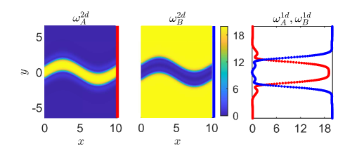
Let be the following sinusoidal function,
with a period of and an amplitude of . After solving the SCF model to obtain the fields and of a one-dimensional planar bilayer, the initial two-dimensional fields and are set as a shift of and . The detailed procedure is provided in Appendix B and an example of this construction is shown in Fig. 2.
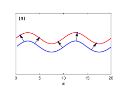
Moreover, the constraint points are chosen from a parallel curve of , as shown in Fig. 3(a). The parallel curve is an extension of along the normal vector . Therefore, the constraint points are of the form , where is half of the planar bilayer’s thickness.
III.3 Extracting the bilayer profile
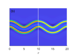
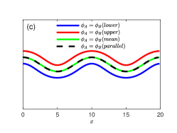
After solving the SCF model with the constraint term, we extract the profile of the bilayer from the convergent concentrations and . A natural way is to use the level set of or . However, the bilayer we considered has two interfaces, which means that the level set, such as , contains two curves. Since there isn’t a standard way to merge the two interfaces into one, we propose several methods to determine the profile and examine the differences later.
The methods include two steps: (1) extracting the upper and lower interface curves, and , parameterized as and , respectively, and (2) merging the two curves into one curve, . It is natural to determine as a level set of , such as . However, the second step is subtle. A simple method can take either or as , and another simple method takes the mean value of and as the parameterization for . Continuing with the concept of parallel surfaces, we present a third method: taking as the curve that is equidistant from and . The detail is provided in Appendix C and the procedure is shown in Fig. 3(b,c).
IV Results and discussion
Now we present the numerical results where the default model parameters are chosen from Cai et al [7] as , . The chemical potential is adjusted so that the planar bilayer is tensionless. The default number of discretization points in space is taken as and , and the number of discretization points in the chain length is . The default numerical parameters are enough to make the results have high accuracies. In addition, the self-consistent fields are updated until the error is less than .
IV.1 Effect of numerical parameters on the energy calculation of the bilayer
In this subsection, we will discuss the effect of numerical parameters on the calculated free energy of the bilayer. The numerical parameters include the number of discretization points or grid size, , , and , for the computational domain and the chain length, respectively, the truncated domain size in the -axis, the number of constraint points, , and the Gaussian constraint width . For the constraint of width, we define a ratio by taking the bilayer’s thickness as a reference width.
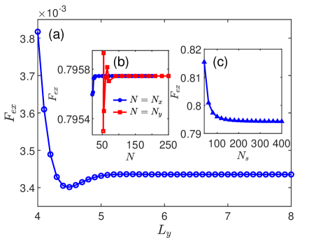
Grid size and domain truncation. It is expected that more discretization points will lead to high accuracy, however, the computation burden is also large. To facilitate the choice of parameters, we compare the free energies calculated under various numerical parameters. Fig. 4 shows the free energy of some demo bilayers as a function of , , , and , respectively. The energy difference is negligible when is larger, for example, , as the concentrations near the boundary are close enough to the bulk phase. In later calculations, when considering the amplitude of the bilayer, we will choose . In addition, the effect of , , and is also negligible when they are large. This implies that our default setting of , , and is already sufficiently large.
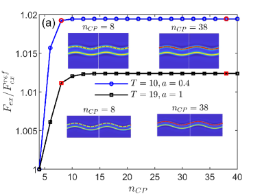
Constraint points and constraint width. Note that the constraint term aims to stabilize bilayers with the desired shape. Using more constraint points is expected to take the membranes close to the target shape, but this will limit the membrane’s self-assembly flexibility. Fig. 5(a) shows the free energy as a function of the number of constraint points. It implies that an increase in the number of constraint points will result in higher free energy, while a smaller number of constraint points is enough to guide the self-assembly of membrane shapes. Therefore, we only use two constraint points, i.e., , in subsequent simulations. This allows the membrane to flexibly adjust its interfaces.
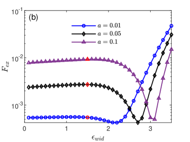
Since the membrane itself has a certain thickness, the non-zero constraint width ratio will affect the final profile of the self-assembled bilayer. Fig. 5(b) shows the effect of on the free energy of bilayers with different amplitudes. It can be observed that the free energy is slightly changed when the ratio is small. To improve the stability of the numerical simulation, we will set in subsequent simulations.
 |
 |
IV.2 Effect of the constraint amplitude and period
Now we start to examine the accuracy of the Helfrich model to predict the excess free energy of periodic cylindrical bilayers with different amplitude and period . As mentioned previously, we consider several methods to determine the profile of the bilayer before evaluating the Helfrich model.
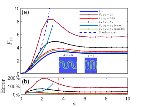
Fig. 6 shows a typical example of bilayers with a fixed period , where the free energy and its relative error are given as a function of the bilayer amplitude . The elastic constants in the Helfrich model are obtained by the asymptotic expansion method [5]. At first, glance, directly taking one level set curve of or , or mean the two-level set curves of as the shape of the bilayer, will lead to a large margin of error, especially when the amplitude is larger. Particularly, the direct mean of the two-level set curves is not feasible when is larger than 3, as the curves are not in the form of . However, using the mean parallel curve as the profile of the bilayer could have better accuracy. In addition, taking the level set curve of also gives good accuracy as it is close to the mean parallel curve.
Since we only used two constraint points, the self-assembled bilayer is not necessarily a standard sinusoidal shape. Fig. 6 also gives the Helfrich energy of sinusoidal curves which is larger than that of the self-assembled bilayers whose profiles are shown in Fig. 6 for and . This agrees with the assumption that the system could adjust the bilayer geometry to decrease the free energy. It is worth noting that the excess free energy of the bilayer remains almost unchanged when is very large. This is because the membrane is flat for a large part, which has small contributions to the whole energy.
 |
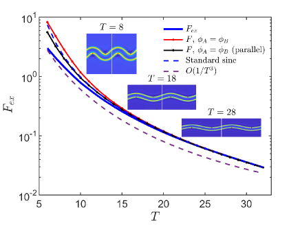 |
Next, we turn to change the period and fix the constraint amplitude . Fig. 7 shows the free energy as a function of and some bilayer profiles. Since the curvature tends to zero when the period tends to infinity, the free energy converges to the surface tension which is zero as we are considering the tensionless bilayer. Helfrich’s energy of standard sinusoidal curves with corresponding amplitude are also compared, which are close to the SCF calculations when is large. This indicates that the prediction of the Helfrich model is accurate when the curve of the periodic cylindrical bilayer is small and the excess free energy is of the order .
IV.3 Effect of the interaction strength
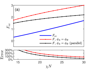
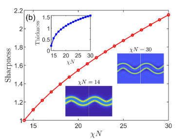
Here, we explore the effect of the interaction strength . As an example, we take and , and show the free energy as a function of in Fig. 8. It is observed that the free energy of bilayers increases almost linearly, which is expected since the bending modulus is almost linearly dependent on [23, 5]. It is interesting to note that the relative prediction error of the Helfrich model decreases when increases. This might be because the bilayer interfaces become sharp and dominate the system. Fig. 8(a,b) gives the bilayers’ sharpness, characterized by and taken the value at as a reference, which is almost linearly increasing. The bilayer’s average thickness is also provided, where the thickness is the distance between two corresponding points on the two interfaces of bilayers. In addition, the shape of several bilayers is also illustrated, which hardly changes for different .
 |
 |
IV.4 Periodic cylindrical bilayers
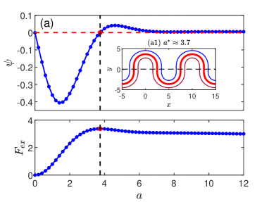
During the numerical simulations, we unexpectedly discovered that there are some equilibrium shapes that satisfy the SCF equations without constraints, i.e., all Lagrange multipliers in Eq. (2) are zero. A typical example of is shown in Fig. 9 by giving the Lagrange multiplier as a function of the constraint amplitude . Note that the Lagrange multiplier vanishes near and the free energy of the bilayer with this critical amplitude achieves the local maximum. The profile of this special is shown in Fig. 9(a1). It is worth noting that this special shape was observed experimentally and subsequently analyzed theoretically as a solution to the shape equations [14, 35, 41].
 |
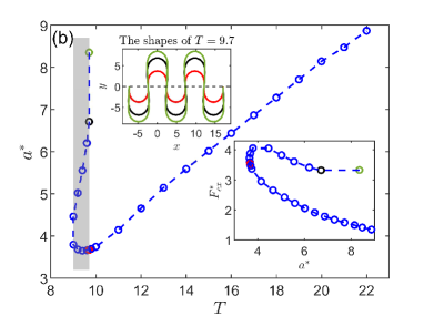 |
Here, we further illustrate that the special bilayer shape is universal for bilayers with different periods. By examining the constraint Lagrange multipliers, we plot the critical amplitudes as a function of the periods in Fig. 9(b). The free energy of bilayers with these critical amplitudes is also provided. When the period is large, such as , the critical amplitude is almost linearly dependent on the period . In addition, the critical shape is the same in the case of where only the scale of the shape changes for different .
However, when is small, such as , there isn’t any critical amplitude. The cases of period between 8.9 and 9.7 seem interesting as there are more than one critical amplitudes . For example, there are three critical amplitudes for the case of as shown in Fig. 9(b). During these multiple critical shapes, the bilayers with large amplitudes have lower free energies.
IV.5 Asymmetic bilayers
Until now, we have been simulating symmetric periodic cylindrical bilayers. However, there are asymmetric bilayers in experiments [25, 22], which are known as the ripple phases of membranes. Here, we asymmetrically assign the constraint points and examine whether the asymmetric bilayers can be in equilibrium states. The two constraint points are located at periodically, where is the ratio of asymmetry and will lead to symmetric constraint points.
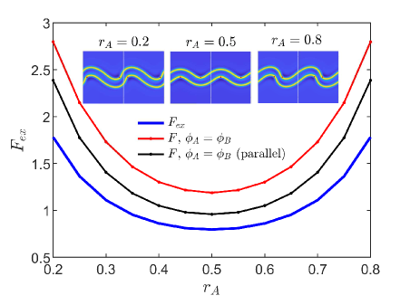
Some examples of asymmetric bilayers are shown in Fig. 10 where the free energy and profiles are given. When the value of is either small or large, the profile of the bilayer differs significantly from that of the symmetric bilayer with . For the case of , we can also obtain equilibrium bilayers by repeating the procedure described in the previous subsection to determine the critical amplitude . Unfortunately, the equilibrium bilayers obtained are symmetric and have the same shape as the bilayer shown in Fig. 9(a1). Note that ripple phases in experiments are observed for lipid bilayers, where the molecules involve rigid or semi-flexible chains. Our simulations suggest that the asymmetric periodic cylindrical bilayers are not equilibrium states for flexible bilayers.
 |
V Conclusion
In this paper, we simulate periodic cylindrical bilayers within the SCF framework and verify the accuracy of the Helfrich model to predict the free energy of self-assembled bilayers. The bilayers are stabilized by introducing some constraint points and the effect of the constraints on the self-assembled bilayers is systematically examined. Numerical results show that the method of reducing the bilayer as a surface is crucial to using the Helfrich model, especially when the bilayer’s curvature is large.
Furthermore, we have identified certain critical bilayers that represent equilibrium states of the SCF model without any constraints. However, the equilibrium bilayers obtained are symmetric, despite the asymmetric assignment of constraint points. This suggests that we should extend the simulation to include periodic liquid-crystalline bilayers, where asymmetric ripple phases have been observed in experiments. A systematic study in this area is intriguing, and we will consider it for future research.
Acknowledgements.
YQ Cai is supported by the National Natural Science Foundation of China (grant no. 12201053). YN Di is partially supported by the National Natural Science Foundation of China (grant no. 12271048), and Guangdong Key Laboratory.Appendix A The bulk phase
The SCF equations have multiple solutions, including the constant solution, which is also known as the bulk phase. In our numerical simulation, the bulk phase is used as the reference state, where its free energy density is given by:
| (17) |
where is the bulk copolymer concentration determined by the following equation:
| (18) |
When Eq. (18) has more than one solution, the one with the lowest free energy density is chosen as the bulk phase.
Appendix B Design the initial fields
In the SCF model, the initial guess of the fields is crucial for efficient simulations. To obtain the periodic cylindrical bilayers, we construct the initial fields based on the results of the one-dimensional planar bilayers. The specific steps are as follows:
-
(1)
Calculate the one-dimensional fields and for tensionless bilayers. Here the chemical potential is adjusted such the bilayer’s excess free energy is zero.
-
(2)
Construct the two-dimensional simulation grid. The computational domain is , which is uniformly discretized as is grid points.
-
(3)
Construct initial guess of the two-dimensional fields and . Denote the two points that satisfying as and , and define their mean value as . Then the two-dimensional fields are assigned as
The evaluation of and is performed using linear interpolation with the values at one-dimensional grid points.
Appendix C Extract the interfaces
We determine the shape of the bilayer based on its order parameters. The following methods are considered:
-
(1)
Take one unilateral level set of , such as the upper part of the set , as the bilayer’s shape.
-
(2)
Directly average the two interfaces such that along -axis as the bilayer’s shape.
-
(3)
Take the parallel median of the two interfaces as the bilayer’s shape.
Here, the parallel median of two interface curves parameterized as is the curve , where and are paired such that the tangent lines of at and , respectively, are parallel.
References
- [1] Alberts, B. Molecular Biology of the Cell. Garland science, 2017.
- [2] Bates, F. S., Hillmyer, M. A., Lodge, T. P., Bates, C. M., Delaney, K. T., and Fredrickson, G. H. Multiblock polymers: Panacea or pandora’s box? Science. 336, 6080 (2012), 434–440.
- [3] Berthault, A., Werner, M., and Baulin, V. A. Bridging molecular simulation models and elastic theories for amphiphilic membranes. J. Chem. Phys. 149, 1 (2018), 014902.
- [4] Binder, K. Monte Carlo and Molecular Dynamics Simulations in Polymer Science. Oxford University Press, 1995.
- [5] Cai, Y.-Q., Li, S.-R., and Shi, A.-C. Elastic properties of self-assembled bilayer membranes: Analytic expressions via asymptotic expansion. J. Chem. Phys. 152, 24 (2020), 244121.
- [6] Cai, Y.-Q., Zhang, P.-W., and Shi, A.-C. Liquid crystalline bilayers self-assembled from rod-coil diblock copolymers. Soft Matter. 13, 26 (2017), 4607–4615.
- [7] Cai, Y.-Q., Zhang, P.-W., and Shi, A.-C. Elastic properties of liquid-crystalline bilayers self-assembled from semiflexible–flexible diblock copolymers. Soft Matter. 15, 45 (2019), 9215–9223.
- [8] Dimova, R. Recent developments in the field of bending rigidity measurements on membranes. Adv. Colloid Interface Sci. 208 (2014), 225–234.
- [9] Flory, P. J. Principles of Polymer Chemistry. Cornell university press, 1953.
- [10] Fredrickson, G. The Equilibrium Theory of Inhomogeneous Polymers. Oxford University Press, 2006.
- [11] Groot, R. D., and Warren, P. B. Dissipative particle dynamics: Bridging the gap between atomistic and mesoscopic simulation. J. Chem. Phys. 107, 11 (1998), 4423–4435.
- [12] Hamley, I. W., et al. Developments in Block Copolymer Science and Technology. Wiley Online Library, 2004.
- [13] Hamm, M., and Kozlov, M. Tilt model of inverted amphiphilic mesophases. The European Physical Journal B-Condensed Matter and Complex Systems. 6 (1998), 519–528.
- [14] Harbich, W., and Helfrich, W. The swelling of egg lecithin in water. Chem. Phys. Lipids. 36, 1 (1984), 39–63.
- [15] Helfand, E. Theory of inhomogeneous polymers: Fundamentals of the gaussian random-walk model. J. Chem. Phys. 62, 3 (1975), 999–1005.
- [16] Helfrich, W. Elastic properties of lipid bilayers: theory and possible experiments. Z. Naturforsch. C. 28, 11 (1973), 693–703.
- [17] Hu, M., Briguglio, J., and Deserno, M. Determining the gaussian curvature modulus of lipid membranes in simulations. Biophys. J. 102, 6 (2012), 1403–1410.
- [18] Jung, H.-S., and Chory, J. Signaling between chloroplasts and the nucleus: Can a systems biology approach bring clarity to a complex and highly regulated pathway? Plant Physiology. 152, 2 (2009), 453–459.
- [19] Kheyfets, B., Galimzyanov, T., Drozdova, A., and Mukhin, S. Analytical calculation of the lipid bilayer bending modulus. Phys. Rev. E. 94, 4 (2016), 042415.
- [20] Korpelainen, H. The evolutionary processes of mitochondrial and chloroplast genomes differ from those of nuclear genomes. Naturwissenschaften. 91, 11 (2004), 505–518.
- [21] Laradji, M., and Desai, R. C. Elastic properties of homopolymer-homopolymer interfaces containing diblock copolymers. J. Chem. Phys. 108, 11 (1998), 4662–4674.
- [22] Lenz, O., and Schmid, F. Structure of symmetric and asymmetric ’ripple’ phases in lipid bilayers. Phys. Rev. Letters. 98, 5 (2007), 058104.1–058104.4.
- [23] Li, J.-F., Pastor, K., Shi, A.-C., Schmid, F., and Zhou, J.-J. Elastic properties and line tension of self-assembled bilayer membranes. Phys. Rev. E. 88, 1 (2013), 012718.
- [24] Liang, Q., Jiang, K., and Zhang, P.-W. Efficient numerical schemes for solving the self-consistent field equations of flexible–semiflexible diblock copolymers. Mathematical Methods in the Applied Sciences. 38, 18 (2015), 4553–4563.
- [25] Lubensky, T. C., and Mackintosh, F. C. Theory of ”ripple” phases of lipid bilayers. Phys. Rev. Letters. 71, 10 (1993), 1565.
- [26] Marsh, D. Elastic curvature constants of lipid monolayers and bilayers. Chem. Phys. Lipids. 144, 2 (2006), 146–159.
- [27] Matsen, M. W. Elastic properties of a diblock copolymer monolayer and their relevance to bicontinuous microemulsion. J. Chem. Phys. 110, 9 (1999), 4658–4667.
- [28] Matsen, M. W. Self-Consistent Field Theory and Its Applications. John Wiley & Sons, Ltd, 2005.
- [29] Matsen, M. W., and Schick, M. Stable and unstable phases of a diblock copolymer melt. Phys. Rev. Letters. 72, 16 (1994), 2660–2663.
- [30] Nagle, J. Introductory lecture: Basic quantities in model biomembranes. Faraday Discuss. 161 (2013), 11–29.
- [31] Noolandi, J., Shi, A.-C., and Linse, P. Theory of phase behavior of poly (oxyethylene)- poly (oxypropylene)- poly (oxyethylene) triblock copolymers in aqueous solutions. Macromolecules. 29, 18 (1996), 5907–5919.
- [32] Ou-Yang, Z.-C., Liu, J.-X., and Xie, Y.-Z. Geometric Methods in the Elastic Theory of Membranes in Liquid Crystal Phases. World Scientific, 1999.
- [33] Palivan, C. G., Goers, R., Najer, A., Zhang, X., Car, A., and Meier, W. Bioinspired polymer vesicles and membranes for biological and medical applications. Chem. Soc. Rev. 45, 2 (2016), 377–411.
- [34] Pivkin, I. V., Caswell, B., and Karniadakisa, G. E. Dissipative particle dynamics. Reviews in Computational Chemistry. 27 (2010), 85–110.
- [35] Shao-Guang, Z., and Ou-Yang, Z.-C. Periodic cylindrical surface solution for fluid bilayer membranes. Phys. Rev. E. 53, 4 (1996), 4206–4208.
- [36] Sodt, A. J., and Pastor, R. W. Bending free energy from simulation: correspondence of planar and inverse hexagonal lipid phases. Biophys. J. 104, 10 (2013), 2202–2211.
- [37] Song, W.-D., Tang, P., Qiu, F., Yang, Y.-L., and Shi, A.-C. Phase behavior of semiflexible-coil diblock copolymers: A hybrid numerical scft approach. Soft Matter. 7, 3 (2011), 929–938.
- [38] Taubert, A., Napoli, A., and Meier, W. Self-assembly of reactive amphiphilic block copolymers as mimetics for biological membranes. Current Opinion in Chemical Biology. 8, 6 (2004), 598–603.
- [39] Thakkar, F. M., Maiti, P. K., Kumaran, V., and Ayappa, K. G. Verifying scalings for bending rigidity of bilayer membranes using mesoscale models. Soft Matter. 7, 8 (2011), 3963–3966.
- [40] Thompson, R. B., Rasmussen, K. O., and Lookman, T. Improved convergence in block copolymer self-consistent field theory by anderson mixing. J. Chem. Phys. 120, 1 (2004), 31–34.
- [41] Tu, Z.-C., and Ou-Yang, Z.-C. Recent theoretical advances in elasticity of membranes following helfrich’s spontaneous curvature model. Adv. Colloid Interface Sci. 208 (2014), 66–75.
- [42] Tzeremes, G., Rasmussen, K., Lookman, T., and Saxena, A. Efficient computation of the structural phase behavior of block copolymers. Phys. Rev. E. 65, 4 (2002), 041806.
- [43] Uneyama, T., and Doi, M. Density functional theory for block copolymer melts and blends. Macromolecules. 38, 1 (2005), 196–205.
- [44] Wang, X.-Y., Li, S.-R., and Cai, Y.-Q. Analytical calculation of the elastic moduli of self-assembled liquid-crystalline bilayer membranes. J. Phys. Chem. B. 125, 20 (2021), 5309–5320.
- [45] Xu, R., Dehghan, A., Shi, A.-C., and Zhou, J.-J. Elastic property of membranes self-assembled from diblock and triblock copolymers. Chem. Phys. Lipids. 221 (2019), 83–92.
- [46] Yu, J.-Y., Liu, F.-Q., Tang, P., Qiu, F., Zhang, H.-D., and Yang, Y.-L. Effect of geometrical asymmetry on the phase behavior of rod-coil diblock copolymers. Polymers. 8, 5 (2016), 184.
- [47] Zhang, P.-W., and Shi, A.-C. Application of self-consistent field theory to self-assembled bilayer membranes. Chin. Phys. B. 24, 12 (2015), 45–52.
- [48] Zhang, P.-W., and Zhang, X.-W. An efficient numerical method of landau–brazovskii model. Journal of Computational Physics. 227, 11 (2008), 5859–5870.