Learning-augmented Online Minimization of Age of Information and Transmission Costs

Abstract

We consider a discrete-time system where a resource-constrained source (e.g., a small sensor) transmits its time-sensitive data to a destination over a time-varying wireless channel. Each transmission incurs a fixed transmission cost (e.g., energy cost), and no transmission results in a staleness cost represented by the Age-of-Information. The source must balance the tradeoff between transmission and staleness costs. To address this challenge, we develop a robust online algorithm to minimize the sum of transmission and staleness costs, ensuring a worst-case performance guarantee. While online algorithms are robust, they are usually overly conservative and may have a poor average performance in typical scenarios. In contrast, by leveraging historical data and prediction models, machine learning (ML) algorithms perform well in average cases. However, they typically lack worst-case performance guarantees. To achieve the best of both worlds, we design a learning-augmented online algorithm that exhibits two desired properties: (i) consistency: closely approximating the optimal offline algorithm when the ML prediction is accurate and trusted; (ii) robustness: ensuring worst-case performance guarantee even ML predictions are inaccurate. Finally, we perform extensive simulations to show that our online algorithm performs well empirically and that our learning-augmented algorithm achieves both consistency and robustness.

I Introduction

In recent years, we have witnessed the swift and remarkable development of the Internet of Things (IoT), which connects billions of entities through wireless networks [2]. These entities range from small, resource-constrained sensors (e.g., temperature sensors and smart cameras) to powerful smartphones. Among various IoT applications, one most important categories is real-time IoT application, which requires timely information updates from the IoT sensors. For example, in industrial automation systems [3, 4], battery-powered IoT sensors are deployed to provide data for monitoring equipment health and product quality. On the one hand, IoT sensors are usually small and have limited battery capacity, and thus frequent transmissions drain the battery quickly; on the other hand, occasional transmissions render the information at the controller outdated, leading to detrimental decisions. In addition, wireless channels can be unreliable due to potential channel fading, interference, and the saturation of wireless networks if the traffic load generated by numerous sensors is high [5]. Clearly, under unreliable wireless networks, IoT sensors must transmit strategically to balance the tradeoff between transmission cost (e.g., energy cost) and data freshness. Other applications include smart grids, smart cities, and so on.

To this end, in the first part of this work, we study the tradeoff between transmission cost and data freshness under a time-varying wireless channel. Specifically, we consider a discrete-time system where a device transmits its data to an access point over an ON/OFF wireless channel (i.e., transmissions occur only when the channel is ON). Each transmission incurs a fixed transmission cost, while no transmission results in a staleness cost represented by the Age-of-Information (AoI) [6], which is defined as the time elapsed since the generation time of the freshest delivered packet. To minimize the sum of transmission costs and staleness costs, we develop a robust online algorithm that achieves a competitive ratio (CR) of $3$. That is, different from typical studies with stationary network assumptions, the cost of our online algorithm is at most three times larger than that of the optimal offline algorithm under the worst channel state (see the definition of CR in Section III).

While online algorithms exhibit robustness against the worst-case situations, they often lean towards excessive caution and may have a subpar average performance in real-world scenarios. On the other hand, by exploiting historical data to build prediction models, machine learning (ML) algorithms can excel in average cases. Nonetheless, ML algorithms could be sensitive to disparity in training and testing data due to distribution shifts or adversarial examples, resulting in poor performance and lacking worst-case performance guarantees.

To that end, we design a novel learning-augmented online algorithm that takes advantage of both ML and online algorithms. Specifically, our learning-augmented online algorithm integrates ML prediction (a series of times indicating when to transmit) into our online algorithm, achieving two desired properties: (i) consistency: when the ML prediction is accurate and trusted, our learning-augmented algorithm performs closely to the optimal offline algorithm, and (ii) robustness: even when the ML prediction is inaccurate, our learning-augmented algorithm still offers a worst-case guarantee.

Our main contributions are as follows.

First, we study the tradeoff between transmission cost and data freshness in a time-varying wireless channel by formulating an optimization problem to minimize the sum of transmission and staleness costs under an ON/OFF channel.

Second, following the approach in [7], we reformulate our (non-linear) optimization problem into a linear Transmission Control Protocol (TCP) acknowledgment problem [8] and propose a primal-dual-based online algorithm that achieves a CR of $3$. While a similar primal-dual-based online algorithm has been claimed to asymptotically achieve a CR of $e/(e-1)$ [7], there is a technical issue in their analysis (see Remark 2).

Third, by incorporating ML predictions into our online algorithm, we design a novel learning-augmented online optimization algorithm that achieves both consistency and robustness. To the best of our knowledge, this is the first study on AoI that incorporates ML predictions into online optimization to achieve consistency and robustness.

Finally, we perform extensive simulations using both synthetic and real trace data. Our online algorithm exhibits better performance than the theoretical analysis, and our learning-augmented algorithm can achieve consistency and robustness.

The remainder of this paper is organized as follows. We first discuss related work in Section II. The system model and problem formulation are described in Section III. In Section IV and Section V, we present our robust online algorithm and our learning-augmented online algorithm, respectively. Finally, we show the numerical results in Section VI and conclude our paper in Section VII.

II Related Work

Since AoI was introduced in [6], it has sparked numerous studies on this topic (see surveys in [9, 10]). Among these AoI studies, two categories are most relevant to our work.

The first category includes studies that consider the joint minimization of AoI and certain costs [11, 12, 13, 14]. The work of [11] studies the problem of minimizing the average cost of sampling and transmission over an unreliable wireless channel subject to average AoI constraints. In [13], the authors consider a source-monitor pair with stochastic arrival of packets at the source. The source pays a transmission cost to send the packet, and its goal is to minimize the weighted sum of AoI and transmission costs. Here the packet arrival process is assumed to follow certain distributions. Although the assumptions in these studies lead to tractable performance analysis, such assumptions may not hold in practical scenarios.

The second category contains studies that focus on non-stationary settings [15, 16, 7, 17]. For example, in [15], the authors proposed online algorithms to minimize the AoI of users in a cellular network under adversarial wireless channels. In these AoI works that consider non-stationary settings, the most relevant work to ours is [7], where the authors study the minimization of the sum of download costs and AoI costs under an adversarial wireless channel. A primal-dual-based randomized online algorithm is shown to have an asymptotic CR of $e/(e-1)$. However, there is a technical issue in their analysis (see Remark 2). To address this issue, we propose an online primal-dual-based algorithm that achieves a CR of $3$ in the non-asymptotic regime. While the AoI optimization problems under non-stationary settings have been investigated, none of them considers applying ML predictions to improve the average performance of online algorithms.

In recent works [18, 19, 20, 21], researchers attempt to take advantage of both online algorithms and ML predictions, i.e., to design a learning-augmented online algorithm that achieves consistency and robustness. In the seminal work [18], by incorporating ML predictions into the online Marker algorithm, the authors can achieve consistency and robustness for a caching problem. Following [18], a large body of research works in this direction have emerged. The most related learning-augmented work to ours is [20], where the authors design a primal-dual-based learning-augmented algorithm for the TCP acknowledgment problem. In [20], the uncertainty comes from the packet arrival times, and the controller can make decisions at any time. In our work, however, the uncertainty comes from the channel states, and no data can be transmitted when the channel is OFF. Lacking the freedom to transmit data at any time makes their algorithm inapplicable.

III System Model and Problem Formulation

System Model. Consider a status-updating system where a resource-limited device sends time-sensitive data to an access point (AP) through an unreliable wireless channel. The system operates in discrete time slots, denoted by $t=1,2,\ldots,T$, where $T$ is finite and is allowed to be arbitrarily large. We use $s(t)\in\{0,1\}$ to denote the channel state at time $t$, where $s(t)=1$ means the channel is ON, allowing the device to access the AP; while $s(t)=0$ means the channel is OFF, preventing access to the AP. The sequence of channel states over the time horizon is represented by $\mathbf{s}=\left\{{s(1),\dots,s(T)}\right\}$.

At the start of each slot, the device probes to know the current channel state and decides whether to transmit its freshest data to the AP. The transmission decision at slot $t$ is denoted by $d(t)\in\{0,1\}$, where $d(t)=1$ if the device decides to transmit (i.e., generates a new update and transmits it to the AP), and $d(t)=0$ if not. A scheduling algorithm $\pi$ is denoted by $\pi=\left\{{{d^{\pi}}(t)}\right\}_{t=1}^{T}$, where ${d^{\pi}}(t)$ is the transmission decisions made by algorithm $\pi$ at time $t$. For simplicity, we use $\pi=\left\{{{d}(t)}\right\}_{t=1}^{T}$ throughout the paper. When the device decides to transmit and the channel is ON, it incurs a fixed transmission cost of $c>1$, and the data on the AP will be successfully updated at the end of slot $t$; otherwise, the data on the AP gets staler. To quantify the freshness of data on the AP side, we utilize a metric called Age-of-Information (AoI) [6], which measures the time elapsed since the freshest received update was generated. We use $a(t)$ to denote the AoI at time $t$, which evolves as

$${a}(t)=\left\{\begin{array}[]{ll}0,&\text{if}\ {s}(t)\cdot{d}(t)=1;\\ {a}(t-1)+1,&\text{otherwise},\end{array}\right.$$ (1)

where the AoI drops to $0$ if the device transmits at ON slots; otherwise, it increases by $1$. Assuming $a(0)=0$. To reflect the penalty when the AP does not get an update at time $t$, we introduce a staleness cost equivalent to the AoI at that time.

Problem Formulation. The total cost of an algorithm $\pi$ is

$$C(\mathbf{s},\pi)\triangleq\sum\limits_{t=1}^{T}{(c\cdot d(t)+a(t))},$$ (2)

where the first item $c\cdot d(t)$ is the transmission cost at time $t$, and the second item $a(t)$ is the staleness cost at time $t$. In this paper, we focus on the class of online scheduling algorithms, under which the information available at time $t$ for making decisions includes the transmission cost $c$, the transmission history $\{d(\tau)\}_{\tau=1}^{t}$, and the channel state pattern $\{s(\tau)\}_{\tau=1}^{t}$, while the time horizon $T$ and the future channel state $\{s(\tau)\}_{\tau={t+1}}^{T}$ is unknown. Conversely, an offline scheduling algorithm has the information about the connectivity pattern $\mathbf{s}$ (and the time horizon $T$) beforehand.

Our goal is to develop an online algorithm $\pi$ that minimizes the total cost given a channel state pattern $\mathbf{s}$:

$$\underset{d(t)}{\min} \sum\limits_{t=1}^{T}{(c\cdot d(t)+a(t))}$$ (3a)

s.t. $$d(t)\in\{0,1\}\ \text{for}\ t=1,2,\dots,T;$$ (3b)

$$a(t)\ \text{evolves as Eq.~{}\eqref{eq:AoI_evo}}\ \text{for}\ t=1,2,\dots,T.$$ (3c)

​​In Problem (3), the only decision variables are the transmission decisions $\{d(t)\}_{t=1}^{T}$, and the objective function is a non-linear function of $\{d(t)\}_{t=1}^{T}$ due to the dependence of $a(t)$ on $d(t)$. Specifically, based on Eq. (1), we can rewrite the AoI at time $t$ as $a(t)=(1-s(t)\cdot d(t))\cdot(a(t-1)+1)$. Upon rephrasing $a(t)$ with the transmission decisions $\{d(\tau)\}_{\tau=1}^{t}$ (i.e., rewriting $a(t-1)$ with $d(t-1)$ and $a(t-2)$, rewriting $a(t-2)$ with $d(t-2)$ and $a(t-3)$, and so forth), we can observe that $a(t)$ involves the products of the current transmission decision $d(t)$ and the previous transmission decisions $d(\tau)$ for $\tau\in[1,t-1]$, which indicates that $a(t)$ is not linear with respect to $\{d(\tau)\}_{\tau=1}^{t}$. This non-linearity poses a challenge to its efficient solutions. In Section IV-A, following a similar line of analysis as in [7], we reformulate Problem (3) to an equivalent TCP acknowledgment (ACK) problem, which is linear and can be solved efficiently (e.g., via the primal-dual approach [22]).

To measure the performance of an online algorithm, we use the metric competitive ratio (CR) [22], which is defined as the worst-case ratio of the cost under the online algorithm to the cost of the optimal offline algorithm. Formally, we say that an online algorithm $\pi$ is $\beta$-competitive if there exists a constant $\beta\geq 1$ such that for any channel state pattern $\mathbf{s}$,

$$C({\bf{s}},\pi)\leq\beta\cdot OPT({\bf{s}}),$$ (4)

where $OPT({\bf{s}})$ is the cost of the optimal offline algorithm for the given channel state $\mathbf{s}$. We desire to develop an online algorithm with a CR close to $1$, which implies that our online algorithm performs closely to the optimal offline algorithm.

IV Robust Online Algorithm

In this section, we first reformulate our AoI Problem (3) to an equivalent linear TCP ACK problem. Then, this TCP ACK problem is further relaxed to a linear primal-dual-based program. Finally, a $3$-competitive online algorithm is developed to solve the linear primal-dual-based program.

IV-A Problem Reformulation

In [7], the authors study the same non-linear Problem (3) and reformulate it to an equivalent linear problem. Following a similar line of analysis as in [7], we reformulate the non-linear Problem (3) to an equivalent linear TCP ACK Problem (5) as follows. Consider a TCP ACK problem, where the source reliably generates and delivers one packet to the destination in each slot $t=1,2,\ldots,T$. Those delivered packets need to be acknowledged (for simplicity, we use “acked” instead of “acknowledged” throughout the paper) that they are received by the destination, which requires the destination to send ACK packets (for brevity, we call it ACK) back to the source. We use $d(t)\in\{0,1\}$ to denote the ACK decision made by the destination at slot $t$. Let $z_{i}(t)\in\{0,1\}$ represent whether packet $i$ (i.e., the packet sent at slot $i$) has been acked by slot $t$ ($i\leq t$), where $z_{i}(t)=1$ if packet $i$ is not acked by slot $t$ and $z_{i}(t)=0$ otherwise. Once packet $i$ is acked at slot $t$, then it is acked forever after slot $t$, i.e., $z_{i}(\tau)=0$ for all $i\leq t$ and all $\tau\geq t$. The feedback channel is unreliable and its channel state in slot $t$ is modeled by an ON/OFF binary variable $s(t)\in\{0,1\}$. We use $\mathbf{s}=\left\{{s(1),\dots,s(T)}\right\}$ to denote the entire feedback channel states. The destination can access the feedback channel state $s(t)$ at the start of each slot $t$. When the feedback channel is ON and the destination decides to send an ACK, all previous packets are acked, i.e., the number of unacked packets becomes $0$; otherwise, the number of unacked packets increases by $1$. We can see that the dynamic of the number of unacked packets is the same as the AoI dynamic.

We assume that there is a holding cost at each slot, which is the number of unacked packets in that slot. In addition, we also assume that each ACK has an ACK cost of $c$. The goal of the TCP ACK problem is to develop an online scheduling algorithm $\pi=\left\{{{d}(t)}\right\}_{t=1}^{T}$ that minimizes the total cost given a feedback channel state pattern $\mathbf{s}$:

$$\underset{d(t),z_{i}(t)}{\min}\hskip 2.84544pt\sum_{t=1}^{T}\left(c\cdot d(t)+\sum_{i=1}^{t}z_{i}(t)\right)$$ (5a)

$$\text{s.t. }\hskip 7.11317ptz_{i}(t)+\sum\nolimits_{\tau=i}^{t}s(\tau)d(\tau)\geq 1$$

$$\hskip 56.9055pt\text{for}\ i\leq t\ \text{and}\ t=1,2,\ldots,T;$$ (5b)

$$\hskip 22.76228ptd(t),z_{i}(t)\in\{0,1\}\ \text{for}\ i\leq t\ \text{and}\ t=1,2,\ldots,T,$$ (5c)

where the first item $c\cdot d(t)$ in Eq. (5a) is the ACK cost at slot $t$, the second item $\sum\nolimits_{i=1}^{t}{{z_{i}}(t)}$ in Eq. (5a) is the holding cost at slot $t$. Constraint (5b) states that for packet $i$ at slot $t$, either this packet is not acked (i.e., $z_{i}(t)=1$) or an ACK was made since its arrival (i.e., $s(\tau)d(\tau)=1$ for some $i\leq\tau\leq t$). While Problem (5) is an integer linear problem, we demonstrate its equivalence to Problem (3) in the following.

Lemma 1.

Problem (5) is equivalent to Problem (3).

We provide detailed proof in Appendix -A and give a proof sketch as follows. We can show that: (i) any feasible solution to Problem (3) can be converted to a feasible solution to Problem (5), and the total costs of these two solutions are the same; (ii) any feasible solution to Problem (5) can be converted to a feasible solution to Problem (3), and the total cost of the converted solution to Problem (3) is no greater than the total cost of the solution to Problem (5). This implies that any optimal solution to Problem (3) is also an optimal solution to Problem (5), and vice versa. Therefore, these two problems are equivalent [23, Sec. 4.1.3].

To obtain a linear program of the integer Problem (5), we relax the integer requirement to real numbers:

$$\underset{d(t),z_{i}(t)}{\min}\hskip 2.84544pt\sum_{t=1}^{T}\left(c\cdot d(t)+\sum_{i=1}^{t}z_{i}(t)\right)$$ (6a)

$$\text{s.t. }\hskip 7.11317ptz_{i}(t)+\sum\nolimits_{\tau=i}^{t}s(\tau)d(\tau)\geq 1$$

$$\hskip 56.9055pt\text{for}\ i\leq t\ \text{and}\ t=1,2,\ldots,T;$$ (6b)

$$\hskip 17.07182pt\ d(t),z_{i}(t)\geq 0\ \text{for}\ i\leq t\ \text{and}\ t=1,2,\ldots,T,$$ (6c)

​which is referred to as the primal problem. The corresponding dual problem of Problem (6) is as follows:

$$\underset{y_{i}(t)}{\max} \sum_{t=1}^{T}\sum_{i=1}^{t}y_{i}(t)$$ (7a)

s.t. $$s(t)\sum_{i=1}^{t}\sum_{\tau=t}^{T}y_{i}(\tau)\leq c\text{ for }t=1,2,\ldots,T;$$ (7b)

$$y_{i}(t)\in[0,1]\text{ for}\ i\leq t\ \text{and}\ t=1,2,\ldots,T,$$ (7c)

​​which has a dual variables $y_{i}(t)$ for packet $i$ and time $t\geq i$.

Remark 1.

In [7], the authors mentioned that their reformulated problem is equivalent to the original AoI problem without proof. For the sake of completeness, we provide rigorous proof regarding the equivalence between Problem (5) and Problem (3) in Lemma 1.

IV-B Primal-dual Online Algorithm Description and Analysis

To solve the primal-dual Problems (6) and (7), we develop the Primal-dual-based Online Algorithm (PDOA) and present it in Algorithm 1. The input is the channel state pattern $\bf{s}$ (revealed in an online manner), and the outputs are the primal variables $d(t)$ and $z_{i}(t)$, and the dual variable $y_{i}(t)$. Two auxiliary variables $L$ and $M$ are also introduced: $L$ denotes the time when the latest ACK was made, and $M$ denotes the ACK marker (PDOA should make an ACK when $M\geq 1$).

PDOA is a threshold-based algorithm. Assuming that the latest ACK was made at slot $L$, when the accumulated holding costs since slot $L+1$ is no smaller than the ACK cost $c$ (i.e., $M\geq 1$), PDOA will make an ACK at the next ON slot $L^{\prime}$. Here, we call the interval $[L+1,L^{\prime}]$ an ACK interval. Note that PDOA updates the primal variables and dual variables only for the packets that are not acked in the current ACK interval $[L+1,L^{\prime}]$. More specifically, consider packet $i$ that has not been acked by the current slot $t\in[L+1,L^{\prime}]$: (i) for the primal variable $z_{i}(t)$, if the threshold is not achieved ($M<1$) or the channel is OFF at slot $t$, PDOA will update $z_{i}(t)$ to be $1$ (in Line 1 or Line 1, respectively) since packet $i$ is not acked by slot $t$; (ii) for the dual variable $y_{i}(t)$, if packet $i$ is not the last packet in the current ACK interval, PDOA will update $y_{i}(t)$ to be $1$ to maximize the dual objective function; otherwise, PDOA will update $y_{i}(t)$ to $c-c\cdot M$ to ensure that when the threshold is achieved ($M\geq 1$), the sum of all the dual variables in the current ACK interval is exactly $c$.

Input : $c$, $\mathbf{s}$ (revealed in an online manner)

Output : $d(t),z_{i}(t),y_{i}(t)$

Init.: $d(t),z_{i}(t),y_{i}(t),L,M\leftarrow 0$ for all $i$ and $t$

1 for $t=1$ to $T$ do

       /* Iterate all the packets arriving since the latest ACK time $L$. */

2       for $i=L+1$ to $t$  do

3             if $M<1$  then /* Not ready to ACK */

4                   ${z_{i}}(t)\leftarrow 1$;

5                   $M\leftarrow M+1/c$;

6                   ${y_{i}}(t)\leftarrow\min\{1,c-c\cdot M\}$;

7                  

8             end if

9             if $M\geq 1$ then /* Ready to ACK */

10                   if $s(t)=1$  then /* ON channel */

11                         $d(t)\leftarrow 1$;

12                         $M\leftarrow 0$;

13                         $L\leftarrow t$;

14                         break and go to the next slot (i.e., $t+1$);

15                        

16                  else /* OFF channel */

17                         ${z_{i}}(t)\leftarrow 1$;

18                        

19                   end if

20                  

21             end if

22            

23       end for

       /* At the end of slot $t$, update dual variable $y_{i}(t)$ with $s(i)=0$ as: */

24       for $i=t$ decrease to $L+1$  do

25             if $s(i)=0$ then

26                   ${y_{i}}(t)\leftarrow 1$;

27                  

28            else

29                  break and go to the next slot;

30             end if

31            

32       end for

33      

34 end for

Algorithm 1 Primal-dual-based Online Algorithm (PDOA)

In addition, at the end of slot $t$ (i.e., Lines 1-1), if the channel is ON at slot $t$, PDOA will skip slot $t$ and go to slot $t+1$. Otherwise, assuming that the most recent ON slot is slot $t^{\dagger}$ ($t^{\dagger}\in[L,t)$), then the channels are OFF during $[t^{\dagger}+1,t]$. To maximize the dual objective function, PDOA updates the dual variables of packet $t^{\dagger}+1$ to packet $t$ to be $1$ since the channels are OFF during $[t^{\dagger}+1,t]$ and the updating of their dual variables does not violate constraint (7b) (see an illustration in Fig. 1(b)). Note that there may be some OFF channels before slot $t^{\dagger}$, but PDOA does not update their dual variables to avoid the violation of constraint (7b). For example, assuming that slot $t^{\prime}$ ($t^{\prime}<t^{\dagger}$) is an OFF channel and we let ${y_{t^{\prime}}}(t)=1$. Letting ${y_{t^{\prime}}}(t)=1$ has no effect on the constraint (7b) at slot $t^{\prime}$ since we always have $s(t^{\prime})\sum_{i=1}^{\hat{t}}\sum_{\tau=t^{\prime}}^{T}y_{i}(\tau)=0$, but doing this does impact the constraint (7b) at slot $t^{\dagger}$ (i.e., increasing $s(t^{\dagger})\sum_{i=1}^{t^{\dagger}}\sum_{\tau=t^{\dagger}}^{T}y_{i}(\tau)$ by $1$ because ${y_{t^{\prime}}}(t)$ is a part of $s(t^{\dagger})\sum_{i=1}^{t^{\dagger}}\sum_{\tau=t^{\dagger}}^{T}y_{i}(\tau)$ as $t^{\prime}<t^{\dagger}$ and $t^{\dagger}\leq t$), possibly making constraint (7b) at slot $t^{\dagger}$ violated.

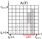
(a) Primal variables $z_{i}(t)$ updates.

(b) Dual variables $y_{i}(t)$ updates.

Figure 1: The updates of primal variables $z_{i}(t)$ and dual variables $y_{i}(t)$ in the $k$-th ACK interval $[t_{k}+1,t_{k+1}]$ of PDOA, where channels are OFF during $[t_{k}+5,t_{k}+7]$. The x-axis represents time and the y-axis represents the packet id. PDOA makes two ACKs at slot $t_{k}$ and slot $t_{k+1}$, where the ACK cost $c=18$. The primal variables $z_{i}(t)$ and dual variables $y_{i}(t)$ are updated from slot $t_{k}+1$ to slot $t_{k+1}$; and in slot $t$, packets are updated from packet $t_{k}+1$ to packet $t$. The red bold italic $1$ denotes when the ACK marker equals or is larger than $1$. In Fig. 1(a), the grey areas denote the updates due to Line 1; In Fig. 1(b), the grey areas denote the updates due to Lines 1-1.

Theorem 1.

PDOA is 3-competitive.

We provide detailed proof in Appendix -B and explain the key ideas as follows. We first show that given any channel state $\bf{s}$, PDOA produces a feasible solution to primal Problem (6) and dual Problem (7). Then, we show that in any $k$-th ACK interval, the ratio between the primal objective value and the dual objective value (denoted by $P(k)$ and $D(k)$, respectively) is at most $3$, i.e., $P(k)/D(k)\leq 3$. This implies that the ratio between the total primal objective value (denoted by $P$) and the total dual objective value (denoted by $D$) is also at most $3$, i.e., $P/D\leq 3$. By the weak duality, PDOA is 3-competitive.

Remark 2.

In [7], the authors also propose a primal-dual-based online algorithm and show that their algorithm achieves a CR of $e/(e-1)$ only when $c$ goes to infinity. In their algorithm, to maximize the dual objective function, at the end of slot $T$, they update certain dual variables $y_{i}(t)$ that arrived at OFF slot to be $1$. In their analysis (specifically, the proof of their Theorem $7$), they show that because of those dual variables updates at the end of slot $T$, the dual objective value is at least $c$ (i.e., $D\geq c$). In addition, the primal objective value satisfies $P\leq(1+1/({(1+1/c)^{\left\lfloor c\right\rfloor}}-1))\cdot D+(T(T+1)/2)\cdot(D/c)$. They claim that when $c$ goes to infinity, this bound becomes $P\leq e/(e-1)\cdot D$ as $(T(T+1)/2)\cdot(D/c)$ goes to $0$. However, this is not true because they already show that $D/c\geq 1$ always holds. Therefore, their analysis cannot lead to the conclusion that their algorithm achieves an asymptotically CR of $e/(e-1)$. Furthermore, when $c$ is finite, their CR is a quadratic function of the time horizon $T$, which can be very large when $T$ is long. Instead, in our algorithm, rather than updating these dual variables $y_{i}(t)$ at the end of slot $T$, we directly update them only in the current ACK interval (i.e., Lines 1-1), ensuring that the dual constraint (7b) is satisfied and the dual objective function is as large as possible. This enables us to focus on the analysis of $P(k)/D(k)$ in the current ACK interval and show that $P(k)/D(k)\leq 3$ for any $k$-th ACK interval, which implies that PDOA is 3-competitive.

V Learning-augmented Online Algorithm

Online algorithms are known for their robustness against worst-case scenarios, but they can be overly conservative and may have a poor average performance in typical scenarios. In contrast, ML algorithms leverage historical data to train models that excel in average cases. However, they typically lack worst-case performance guarantees when facing distribution shifts or outliers. To attain the best of both worlds, we design a learning-augmented online algorithm that achieves both consistency and robustness.

V-A Machine Learning Predictions

We consider the case where an ML algorithm provides a prediction $\mathcal{P}\triangleq\{{p_{1}},{p_{2}},\dots,{p_{n}}\}$ that represents the times to transmit an ACK for the destination (i.e., the prediction $\mathcal{P}$ makes a total of $n$ ACKs and sends the $i$-th ACK at slot $p_{i}$). The prediction $\mathcal{P}$ is unaware of the channel state pattern $\mathbf{s}$ and can be provided either in full in the beginning (i.e., $t=0$) or be provided one-by-one in each slot. Furthermore, when the prediction $\mathcal{P}$ decides to send an ACK at an OFF slot, we will simply ignore the decision for this particular slot.

Provided with the prediction $\mathcal{P}$, we specify a trust parameter $\lambda\in(0,1]$ to reflect our confidence in the prediction: a smaller $\lambda$ means higher confidence. The learning-augmented online algorithm takes a prediction $\mathcal{P}$, a trust parameter $\lambda$, and a channel state pattern $\mathbf{s}$ (revealed in an online manner) as inputs, and outputs a solution with a cost of $C(\mathbf{s},\mathcal{P},\lambda)$. A learning-augmented algorithm is said $\beta(\lambda)$-robust ($\beta(\lambda)\geq 1$) and $\gamma(\lambda)$-consistent ($\gamma(\lambda)\geq 1$) if its cost satisfies

$$C(\mathbf{s},\mathcal{P},\lambda)\leq\min\{\beta(\lambda)\cdot OPT(\mathbf{s}),\gamma(\lambda)\cdot C(\mathbf{s},\mathcal{P})\},$$ (8)

where $OPT(\mathbf{s})$ and $C(\mathbf{s},\mathcal{P})$ is the cost of the optimal offline algorithm and the cost of purely following the prediction $\mathcal{P}$ under the channel state pattern $\mathbf{s}$, respectively.

We aim to design a learning-augmented online algorithm for primal Problem (6) that exhibits two desired properties (i) consistency: when the ML prediction $\mathcal{P}$ is accurate ($C(\mathbf{s},\mathcal{P})\approx OPT(\mathbf{s})$) and we trust it, our learning-augmented online algorithm should perform closely to the optimal offline algorithm (i.e., $\gamma(\lambda)\to 1$ as $\lambda\to 0$); and (ii) robustness: even if the ML prediction $\mathcal{P}$ is inaccurate, our learning-augmented online algorithm still retains a worst-case guarantee (i.e., $C(\mathbf{s},\mathcal{P},\lambda)\leq\beta(\lambda)\cdot OPT(\mathbf{s})$ for any prediction $\mathcal{P}$).

Input : $c$, $\mathcal{P},\lambda$, $\mathbf{s}$ (revealed in an online manner)

Output : $d(t),z_{i}(t),y_{i}(t)$

Init.: $d(t),z_{i}(t),y_{i}(t),L,M\leftarrow 0$ for all $i$ and $t$

1 for $t=1$ to $T$ do

       /* Iterate all the packets arriving since the most recent ACK time $L$. */

2       for $i=L+1$ to $t$  do

3             if $M<1$  then /* Not ready to ACK */

4                   if $t\geq\alpha(i)$ then

                         /* Big update: prediction already acked packet $i$ */

5                         $M^{\prime}\leftarrow 1/{\lambda c}$, $y^{\prime}\leftarrow 1$;

6                        

7                  else

                         /* Small update: prediction did not ack packet $i$ yet */

8                         $M^{\prime}\leftarrow\lambda/c$, $y^{\prime}\leftarrow\lambda$;

9                        

10                   end if

11                  ${z_{i}}(t)\leftarrow 1$;

12                   $M\leftarrow M+M^{\prime}$;

13                   ${y_{i}}(t)\leftarrow y^{\prime}$;

14                  

15             end if

16            if $M\geq 1$ then /* Ready to ACK */

17                   if $s(t)=1$ then /* ON channel */

18                         $d(t)\leftarrow 1$;

19                         $M\leftarrow 0$;

20                         $L\leftarrow t$;

21                         break and go to the next slot (i.e., $t+1$);

22                        

23                  else /* OFF channel */

24                        if ${z_{i}}(t)\neq 1$ then

                               /* Zero update */

25                               ${z_{i}}(t)\leftarrow 1$;

26                              

27                         end if

28                        

29                   end if

30                  

31             end if

32            

33       end for

       /* At the end of slot $t$, update dual variable $y_{i}(t)$ with $s(i)=0$ as: */

34       for $i=t$ decrease to $L+1$  do

35             if $s(i)=0$ then

36                   if ${y_{i}}(t)=0$ then

37                        ${y_{i}}(t)\leftarrow 1$;

38                   end if

39                  

40            else

41                  break and go to the next slot;

42             end if

43            

44       end for

45      

46 end for

Algorithm 2 Learning-augmented Primal-dual-based Online Algorithm (LAPDOA)

V-B Learning-augmented Online Algorithm Description

We present our Learning-augmented Primal-dual-based Online Algorithm (LAPDOA) in Algorithm 2. LAPDOA behaves similarly to PDOA, but the updates of primal variables and dual variables incorporate the ML prediction $\mathcal{P}$.

In LAPDOA, two additional auxiliary variables $M^{\prime}$ and $y^{\prime}$ are used to denote the increment of the ACK marker $M$ and the increment of the dual variables $y_{i}(t)$ in each iteration of update, respectively. Assuming that the current time is $t$, let $\alpha(t)$ denote the next time when the prediction $\mathcal{P}$ sends an ACK (i.e., $\alpha(t)\triangleq\min\{{p_{i}}:{p_{i}}\geq t\}$ and $\alpha(t)=\infty$ if $t>{p_{n}}$). For the updates of primal and dual variables of an unacked packet $i$ at slot $t$, based on the relationship between the current time $t$ and $\alpha(i)$ (which is also the time when the prediction $\mathcal{P}$ makes an ACK for packet $i$ because packet $i$ arrives at slot $i$), we classify them into three types:

• Big updates: those updates make $M^{\prime}\leftarrow 1/\lambda c$, $y^{\prime}\leftarrow 1$, and $z_{i}(t)\leftarrow 1$. The big updates are made when LAPDOA is behind the ACK scheduled by the prediction $\mathcal{P}$ (i.e., $t\geq\alpha(i)$), and it tries to catch up the prediction $\mathcal{P}$ by making a big increase in the ACK marker.

• Small updates: those updates make $M^{\prime}\leftarrow\lambda/c$, $y^{\prime}\leftarrow\lambda$, and $z_{i}(t)\leftarrow 1$. The small updates are made when LAPDOA is ahead of the ACK scheduled by the prediction $\mathcal{P}$ (i.e., $t<\alpha(i)$), and LAPDOA tries to slow down its ACK rate by making a small increase in the ACK marker.

• Zero updates: those updates make $M^{\prime}\leftarrow 0$, $y^{\prime}\leftarrow 0$, and $z_{i}(t)\leftarrow 1$. The zero updates are made when LAPDOA is supposed to ACK at some slot $t^{\prime}$ but finds that slot $t^{\prime}$ is OFF, and it has to delay its ACK to the next ON slot and pay the holding cost (i.e., $z_{i}(t)=1$) along the way.

An illustration of these three types of updates is in Fig. 2.

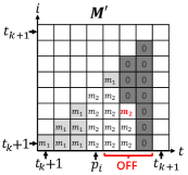
(a) Auxiliary variables $M^{\prime}$ updates.

(b) Primal variables $z_{i}(t)$ updates.

(c) Dual variables $y_{i}(t)$ updates.

Figure 2: The updates of variables in the $k$-th ACK interval $[t_{k}+1,t_{k+1}]$ of LAPDOA, where channels are OFF during $[t_{k}+5,t_{k}+7]$. LAPDOA makes two ACKs at $t_{k}$ and $t_{k+1}$, and the ML prediction $\mathcal{P}$ makes its $i$-th ACK at slot $t_{k}+4$. The red bold italic value denotes when the ACK marker $M\geq 1$. Let ${m_{1}}=\lambda/c$, ${m_{2}}=1/\lambda c$, ${y_{1}}=\lambda$, and ${y_{2}}=1$. The light grey area denotes the small updates, the white area (without background) denotes the big updates, and the dark grey area denotes the zero updates.

V-C Learning-augmented Online Algorithm Analysis

In this subsection, we focus on the consistency and robustness analysis of LAPDOA with $\lambda\in(0,1]$. The special cases of LAPDOA with $\lambda=0$ and $\lambda=1$ correspond to the cases that LAPDOA follows the prediction $\mathcal{P}$ purely and PDOA, respectively. It is noteworthy that by choosing different values of $\lambda$, LAPDOA exhibits a crucial trade-off between consistency and robustness.

Theorem 2.

For any channel state pattern $\mathbf{s}$, any prediction $\mathcal{P}$, any parameter $\lambda\in(0,1]$, and any ACK cost $c$, LAPDOA outputs an almost feasible solution (within a factor of $c/(c+1)$) with a cost of: when $\lambda\in(0,1/c]$,

$${C}({\mathbf{s}},{\cal P},\lambda)\leq \min\{({3}/{\lambda})\cdot(({{c+1}})/{c})\cdot OPT({\mathbf{s}}),$$

$$(1+\lambda){C_{H}}({\mathbf{s}},{\cal P})+{C_{A}}({\mathbf{s}},{\cal P})\},$$ (9)

and when $\lambda\in(1/c,1]$,

$$C(\mathbf{s},\mathcal{P},\lambda)\leq\min\{({3}/{\lambda})\cdot(({{c+1}})/{c})\cdot OPT({\mathbf{s}}),$$

$$(\lambda+2)C_{H}(\mathbf{s},\mathcal{P})+(1/\lambda+2)\cdot\left\lceil{\lambda c}\right\rceil\cdot C_{A}(\mathbf{s},\mathcal{P})/{c}\},$$ (10)

where $C_{A}(\mathbf{s},\mathcal{P})$ and $C_{H}(\mathbf{s},\mathcal{P})$ denote the total ACK costs and total holding costs of prediction $\mathcal{P}$ under $\mathbf{s}$, respectively; and $C(\mathbf{s},\mathcal{P})=C_{A}(\mathbf{s},\mathcal{P})+C_{H}(\mathbf{s},\mathcal{P})$.

Next, we show that LAPDOA has the robustness guarantee in Lemma 11 and the consistency guarantee in Lemma 3. Combining Lemmas 11 and 3, we can conclude Theorem 2.

Lemma 2.

(Robustness) For any ON/OFF input instance $\mathbf{s}$, any prediction $\mathcal{P}$, any parameter $\lambda\in(0,1]$, and any ACK cost $c$, LAPDOA outputs a solution which has a cost of

$$C(\mathbf{s},\mathcal{P},\lambda)\leq(3/\lambda)\cdot((c+1)/c)OPT(\mathbf{s}).$$ (11)

We provide detailed proof in Appendix -C and explain the key ideas as follows. We first show that LAPDOA produces a feasible primal solution and an almost feasible dual solution (with a factor of $c/(c+1)$). Then, we show that in any $k$-th ACK interval, LAPDOA achieves $P(k)/{D}(k)\leq 3/\lambda$. This implies that LAPDOA also achieves $P/{D}\leq 3/\lambda$ on the entire instance. Finally, by scaling down all dual variables ${y_{i}}(t)$ generated by LAPDOA by a factor of $c/(c+1)$, we obtain a feasible dual solution with a dual objective value of $(c/(c+1))\cdot D$. By the weak duality, we have $P/OPT\leq P/((c/(c+1))\cdot D)=(P/D)\cdot((c+1)/c)\leq(3/\lambda)\cdot((c+1)/c)$.

Lemma 3.

(Consistency) For any channel state pattern $\mathbf{s}$, any prediction $\mathcal{P}$, any parameter $\lambda\in(0,1]$, and any ACK cost $c$, LAPDOA outputs a solution with a cost of: when $\lambda\in(0,1/c]$,

$$C(\mathbf{s},\mathcal{P},\lambda)\leq(1+\lambda)C_{H}(\mathbf{s},\mathcal{P})+C_{A}(\mathbf{s},\mathcal{P}),$$ (12)

and when $\lambda\in(1/c,1]$,

$$C(\mathbf{s},\mathcal{P},\lambda)\leq$$

$$(\lambda+2)C_{H}(\mathbf{s},\mathcal{P})+(1/\lambda+2)\cdot\left\lceil{\lambda c}\right\rceil\cdot{C_{A}(\mathbf{s},\mathcal{P})}/{c},$$ (13)

where $C_{A}(\mathbf{s},\mathcal{P})$ and $C_{H}(\mathbf{s},\mathcal{P})$ denote the total ACK cost and total holding cost of prediction $\mathcal{P}$ under $\mathbf{s}$, respectively; and $C(\mathbf{s},\mathcal{P})=C_{A}(\mathbf{s},\mathcal{P})+C_{H}(\mathbf{s},\mathcal{P})$.

We provide detailed proof in Appendix -D and give a proof sketch as follows. In general, LAPDOA generates three types of updates: big updates, small updates, and zero updates. Our idea is to bound the total cost of each type of update by the cost of the algorithm that purely follows the prediction. In the case of $\lambda\in(0,1/c]$, we show that the total number of big updates is $C_{A}(\mathbf{s},\mathcal{P})/c$, and each big update increases the primal objective value by $c$, so the total cost of big updates in LAPDOA is $C_{A}(\mathbf{s},\mathcal{P})$. In addition, the total number of small updates and zero updates can be shown to be bounded by $C_{H}(\mathbf{s},\mathcal{P})$, and each small update or zero update incurs a cost at most $1+\lambda$, thus the total cost of small and zero updates in LAPDOA is at most $(1+\lambda)C_{H}(\mathbf{s},\mathcal{P})$. In summary, the total cost of LAPDOA in the case of $\lambda\in(0,1/c]$ is bounded by $(1+\lambda)C_{H}(\mathbf{s},\mathcal{P})+((c+1)/c)C_{A}(\mathbf{s},\mathcal{P})$. A similar bound can be also obtained for the case of $\lambda\in(1/c,1]$.

Remark 3.

When we trust the ML prediction (i.e., $\lambda\to 0$) and the ML prediction is accurate at the same time ($C(\mathbf{s},\mathcal{P})\approx OPT(\mathbf{s})$), our learning-augmented algorithm also performs nearly to the optimal offline algorithm, achieving consistency.

Remark 4.

With any $\lambda\in(0,1]$, the CR of LAPDOA is at most $(3/\lambda)\cdot((c+1)/c)$, regardless of the prediction quality. This indicates that our learning-augmented algorithm has the worst-case performance guarantees, achieving robustness.

VI Numerical Results

In this section, we perform simulations using both synthetic data and real trace data to show that our online algorithm PDOA outperforms the State-of-the-Art online algorithm and that our learning-augmented online algorithm LAPDOA achieves consistency and robustness.

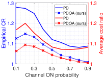
(a) Bernoulli process

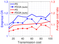
(b) Real trace dataset

Figure 3: Performance comparison of online algorithms under different datasets.

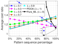
Figure 4: Performance comparison of LAPDOA under different trust parameters using synthetic dataset.

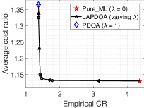
Figure 5: Average cost ratio vs. empirical CR of LAPDOA when the pattern sequence percentage is $99\%$. The direction of the arrow indicates that $\lambda$ becomes larger.

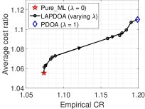
(a) Driving tests (small shift)

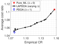
(b) Walking tests (big shift)

Figure 6: Average cost ratio vs. empirical CR of LAPDOA using real trace dataset. The direction of the arrow indicates that $\lambda$ becomes larger.

VI-A Online Algorithm

In Fig. 4, we compare PDOA with the State-of-the-Art online algorithm proposed in [7] (which is referred to as “PD” in Fig. 4). Two datasets are considered: (i) The synthetic dataset in Fig. 3(a). We adopt the same settings as in [7], where the channel state is a Bernoulli process with varying channel ON probability and the transmission cost $c=15$; (ii) The real trace dataset [24] in Fig. 3(b). This dataset contains the channel measurement (i.e., reference signal received quality (RSRQ)) of the commercial mmWave 5G services in a major U.S. city. Specifically, located in the Minneapolis downtown region, the researchers in [24] repeatedly conduct walking tests on the 1300m loop area. Throughout these walking tests, they utilized a 5G monitoring tool installed on an Android smartphone to collect RSRQ information. The RSRQ values fluctuate as the tester moves, being higher in proximity to the mmWave 5G tower and decreasing as the tester moves away from it. For the ON/OFF channel determination, a threshold is established for the RSRQ (-13dB): the channel is considered ON when the RSRQ exceeds the threshold; otherwise, it is deemed OFF. Here we vary the transmission cost from $10$ to $100$. In both datasets, the performance metrics are the empirical CR and the average cost ratio (i.e., the worst cost ratio and the average cost ratio under the online algorithm and the optimal offline algorithm over multiple simulation runs).

Fig. 4 illustrates that our online algorithm PDOA consistently outperforms the State-of-the-Art online algorithm PD in both datasets, i.e., PDOA achieves a lower empirical CR and a lower average cost ratio compared to PD. In addition, the empirical CR of PDOA outperforms the theoretical analysis (with a CR of 3), validating our theoretical results.

VI-B Learning-augmented Online Algorithm

In this subsection, we study the performance of LAPDOA under different prediction qualities using both synthetic datasets and real trace datasets. We first explain how to generate ML predictions based on the training dataset. Then, we shift the distribution of the testing dataset to deviate from the training dataset and showcase the performance of LAPDOA on the testing datasets.

The Synthetic Dataset. In Fig. 3(a), PDOA demonstrates strong performance under the Bernoulli process. However, a specific training dataset reveals its suboptimal performance. In this training dataset, the transmission cost $c=16$, and the channel state sequence is constituted by an independently repeating pattern [$X\times$OFF, $Y\times$ON], where $X\sim B(13,0.9)$ and $Y\sim B(6,0.9)$ ($B(n,p)$ represents the binomial distribution with parameters $n$ and $p$). Under this pattern, in most cases, PDOA only makes one transmission at the first ON slot of these $Y$ ON slots (i.e., after a long consecutive $X$ OFF slots, the ACK marker $M$ will be larger than $1$, and PDOA will transmit at the first ON slot. However, after this transmission, during the short remaining $(Y-1)$ ON slots, the ACK marker $M$ is unable to be increased to $1$). This results in a high AoI increase for these next $X$ OFF slots. While for the optimal offline algorithm, to have a lower AoI increase during OFF slots, it will transmit at both the first ON slot and the last ON slot among those $Y$ ON slots. To generate a sequence of channel states of the required length, we repeat the pattern enough times independently and concatenate them together.

Recall that LAPDOA incorporates an ML prediction $\mathcal{P}$ that provides the transmission decision at each slot. To generate such an ML prediction $\mathcal{P}$, we train an Long Short-term Memory (LSTM) network, which has three LSTM layers (each layer has $20$ hidden states) followed by one fully connected layer. The input of our LSTM network is the current channel state, and the output is the transmission probability at that slot. For training, we manually create 300 sequences, each with a length of 100 slots consisting of repeating patterns introduced earlier (we call these constructed sequences “pattern sequences”). Optimal offline transmission decisions for the training datasets are obtained through dynamic programming. We use the mean squared error between the LSTM network output and the optimal offline algorithm output as the loss function and employ the Adam optimizer to train the weights. In the end, to convert the output of our LSTM network (i.e., transmission probability) to the real transmission decisions, a threshold (e.g., $0.5$) is set, and transmission occurs when the output of the LSTM network exceeds the threshold.

In Fig. 4, we illustrate LAPDOA’s performance under varying prediction qualities, influenced by a distribution shift between the training and testing datasets. The training dataset only contains the sequences that are fully composed of the pattern (i.e., the percentage of the pattern sequences is $100\%$). However, in the testing dataset, we reduce the percentage of the pattern sequence by replacing some pattern sequences with a Bernoulli process sequence of a length of $100$ with an ON probability of $0.32$ (close to the pattern ON probability). While the training dataset and the testing dataset share the same channel ON probability, they exhibit shifts in distribution. The magnitude of this shift amplifies as the percentage of the pattern sequence decreases. As we can observe in Fig. 4, when the distribution shift is small ($100\%$ or $90\%$ pattern sequence percentage), our trained ML algorithm (“Pure_ML” in the figure) outperforms PDOA (recall that Pure_ML is a special case of LAPDOA with $\lambda=0$, and PDOA is a special case of LAPDOA with $\lambda=1$). Learning-augmented algorithms trusting the prediction ($\lambda\in\{0.1,0.3\}$) closely match the ML algorithm’s performance. Conversely, with a substantial distribution shift ($0$ or $10\%$ pattern sequence percentage), the ML algorithm performs poorly while PDOA performs well. In this case, learning-augmented algorithms not trusting the prediction ($\lambda\in\{0.7,0.9\}$) closely resemble PDOA. Furthermore, with different values of $\lambda$, LAPDOA provides different tradeoff curves for consistency and robustness.

Though the trained ML algorithm performs well in the average case when the distribution shift is small (i.e., Pure_ML achieves a low average cost ratio in Fig. 4 when the pattern sequence percentage is high), it may lack worst-case performance guarantees. In Fig. 6, we show the comparison between the average cost ratio and the empirical CR under LAPDOA when the pattern sequence percentage is $99\%$ (i.e., there exists at least a sequence that is not the pattern sequence). Here we consider the LAPDOA algorithms with $\lambda\in\{0,0.1,...,0.9,1\}$. Pure_ML achieves the smallest average cost ratio, however, its empirical CR significantly surpasses that of PDOA, indicating that it lacks performance robustness. In addition, as the trust parameter $\lambda$ increases, the empirical CR performance improves, while the performance of the average cost ratio worsens. In this scenario, selecting $\lambda$ as $0.3$ appears to be beneficial, as it not only yields a low empirical CR but also sustains a low average cost ratio concurrently.

The Real Trace Dataset. We still use the real trace dataset [24]. In addition to the walking tests we introduced before, this dataset also contains the RSRQ measurement of the driving tests. Throughout these driving tests, the researchers mounted the smartphone on the car’s windshield and repeatedly drove on the same 1300m loop area to collect RSRQ information. Again, we set a threshold for RSRQ ($-13$dB) to determine the ON/OFF channels. The differences between the driving datasets and the walking datasets are that: (i) the time length of one driving loop is much shorter than that of one walking loop (i.e., 250 seconds vs 750 seconds); (ii) the number of ON slots in the driving dataset is less than that in the walking dataset. As explained in [24], this phenomenon primarily arises due to signal attenuation caused by the car’s body components, such as windshields or side windows. Additionally, the swift movement of the car leads to frequent handoffs between 5G panels and towers, which further degrades signal strength.

Similar to the synthetic dataset, the ML prediction $\mathcal{P}$ is also generated by an LSTM network (with the same architecture as introduced in the synthetic dataset). To train this LSTM network, we use a $5$ loop of driving tests as our training dataset. We consider two different testing datasets: (i) a $3$ loop of driving tests in Fig. 6(a), and (ii) a $3$ loop of walking tests in Fig. 6(b). The distribution shift between the first testing dataset and the training dataset is small as the data is collected under the same scenario (i.e., driving), while the distribution shift between the second testing dataset and the training dataset is large as the data is collected under the two different scenarios (i.e., walking vs. driving). In Fig. 6(a), when the testing dataset is the driving dataset, which has a small distribution shift compared to the training dataset, the Pure_ML demonstrates superior performance not only for average cost ratio but also empirical CR. We conjecture that Pure_ML achieves a low empirical CR because this testing dataset is highly identical to the training datasets (i.e., with the same $1300$m loop area, the signal strength measured in one driving loop does not appear to change dramatically in another driving loop, and thus those driving loops share a similar signal strength pattern). However, in Fig. 6(b), when the testing dataset significantly deviates from the training dataset, the performance of Pure_ML diminishes, resulting in both a high average cost ratio and a high empirical CR. In contrast, the PDOA online algorithm excels in this scenario in terms of both the average cost ratio and the empirical CR. Upon analyzing these two testing datasets, we learn that, on the one hand, if we possess an understanding of the characteristics in the testing dataset, we can select our trust parameters correspondingly. For example, if we are aware that the testing dataset deviates from the training dataset greatly, we should choose a lower trust parameter. On the other hand, when uncertainty shrouds the testing dataset, selecting an appropriate trust parameter (e.g., $\lambda=0.3$) enables LAPDOA to strike a good trade-off between consistency and robustness.

VII Conclusion

In this paper, we studied the minimization of data freshness and transmission costs under a time-varying wireless channel. After reformulating our original problem to a TCP ACK problem, we developed a $3$-competitive primal-dual-based online algorithm. Realizing the pros and cons of online algorithms and ML algorithms, we designed a learning-augmented online algorithm that takes advantage of both approaches and achieves consistency and robustness. Finally, simulation results validate the superiority of our online algorithm and highlight the consistency and robustness achieved by our learning-augmented algorithm. For future work, one interesting direction would be to consider how to adaptively select the trust parameter $\lambda$ to achieve the best performance.

-A Proof of Lemma 1

Proof.

Our goal is to show that: (i) any feasible solution to Problem (3) can be converted to a feasible solution to Problem (5), and the total costs of these two solutions are the same; (ii) any feasible solution to Problem (5) can be converted to a feasible solution to Problem (3), and the total cost of the converted solution to Problem (3) is no greater than the total cost of the solution to Problem (5). With above two statements, we can show that any optimal solution to Problem (3) is also an optimal solution to Problem (5), and vice versa. Therefore, these two problems are equivalent [23, Sec. 4.1.3].

We first show that any feasible solution to Problem (3) can be converted to a feasible solution to Problem (5). Given a channel state pattern $\mathbf{s}$, we assume that the solution $\pi=\{{t_{1}},{t_{2}},\dots,{t_{n}}\}$ is a feasible solution to Problem (3), where this solution makes the $i$-th transmission at the ON slot $t_{i}$ (i.e., $s(t_{i})d(t_{i})=1$), and the total number of transmission is $n$. We can compute the total cost of the solution $\pi$ to Problem (3) as ${C_{\ref{problem}}}(s,\pi)=cn+({t_{1}}-1){t_{1}}/2+\sum\nolimits_{i=2}^{n}{({t_{i}}-{t_{i-1}}-1)({t_{i}}-{t_{i-1}})/2}+(T-{t_{n}}-1)(T-{t_{n}})/2$, where $cn$ is the total transmission cost and the rest is the total staleness cost. Based on the solution $\pi$ to Problem (3), we construct a solution $\pi^{\prime}$ to Problem (5) in the following way: (i) solution $\pi^{\prime}$ sends the ACKs at the same time when solution $\pi$ transmits, i.e., solution $\pi^{\prime}$ sends ACKs at a sequence of slots $\{t{{}_{1}},t{{}_{2}},\dots,t{{}_{n}}\}$; (ii) based on the ACK decisions in step (i), for any slot $t$ and any packet $i\leq t$, solution $\pi^{\prime}$ lets $z_{i}(t)=0$ if $\sum\nolimits_{\tau=i}^{t}s(\tau)d(\tau)\geq 1$ and $z_{i}(t)=1$ if $\sum\nolimits_{\tau=i}^{t}s(\tau)d(\tau)=0$. We denote the solution $\pi^{\prime}$ to Problem (5) by $\pi^{\prime}=\{\{{t_{1}},{t_{2}},\dots,{t_{n}}\},\{\{{z_{i}}(t)\}_{i=1}^{t}\}_{t=1}^{T}\}$. We can easily verify that solution $\pi^{\prime}$ is a feasible solution to Problem (5) because both constraints (5b) and (5c) are satisfied. Furthermore, according to the construction of $z_{i}(t)$ in step (ii), we know that once the ACK is made at some ON slot $t\in\{{t_{1}},{t_{2}},\dots,{t_{n}}\}$, then all previously arrived packets (packet $1$ to packet $t$) are acked forever after slot $t$, i.e., $z_{i}(\tau)=0$ for all $i\leq t$ and all $\tau\geq t$. This indicates that we can compute the total holding cost of the solution $\pi^{\prime}$ as

$$\sum\nolimits_{t=1}^{T}{\sum\nolimits_{i=1}^{t}{{z_{i}}(t)}}$$

$$= \underbrace{\sum\nolimits_{t=1}^{{t_{1}}-1}{\sum\nolimits_{i=1}^{t}{{z_{i}}(t)}}+\sum\nolimits_{t={t_{1}}}^{T}{\sum\nolimits_{i=1}^{{t_{1}}}{{z_{i}}(t)}}}_{\text{Total holding cost of packet $1$ to packet $t_{1}$}}$$

$$+\underbrace{\sum\nolimits_{t={t_{1}}+1}^{{t_{2}}-1}{\sum\nolimits_{i={t_{1}}+1}^{t}{{z_{i}}(t)}}+\sum\nolimits_{t={t_{2}}}^{T}{\sum\nolimits_{i={t_{1}}+1}^{{t_{2}}}{{z_{i}}(t)}}}_{\text{Total holding cost of packet ($t_{1}+1$) to packet $t_{2}$}}$$

$$+\dots+\underbrace{\sum\nolimits_{t={t_{n}}+1}^{T}{\sum\nolimits_{i={t_{n}}+1}^{t}{{z_{i}}(t)}}}_{\text{Total holding cost of packet ($t_{n}+1$) to packet $T$}}$$

$$\buildrel(a)\over{=} \underbrace{\sum\nolimits_{t=1}^{{t_{1}}-1}{\sum\nolimits_{i=1}^{t}{1}}+\sum\nolimits_{t={t_{1}}}^{T}{\sum\nolimits_{i=1}^{{t_{1}}}{0}}}_{\text{Total holding cost of packet $1$ to packet $t_{1}$}}$$ (14)

$$+\underbrace{\sum\nolimits_{t={t_{1}}+1}^{{t_{2}}-1}{\sum\nolimits_{i={t_{1}}+1}^{t}{1}}+\sum\nolimits_{t={t_{2}}}^{T}{\sum\nolimits_{i={t_{1}}+1}^{{t_{2}}}{0}}}_{\text{Total holding cost of packet ($t_{1}+1$) to packet $t_{2}$}}$$

$$+\dots+\underbrace{\sum\nolimits_{t={t_{n}}+1}^{T}{\sum\nolimits_{i={t_{n}}+1}^{t}{1}}}_{\text{Total holding cost of packet ($t_{n}+1$) to packet $T$}}$$

$$= ({t_{1}}-1){t_{1}}/2+\sum\nolimits_{i=2}^{n}{({t_{i}}-{t_{i-1}}-1)({t_{i}}-{t_{i-1}})/2}$$

$$+(T-{t_{n}}-1)(T-{t_{n}})/2,$$

where in (a), ${z_{i}}(t)=1$ is because packet $i$ is not acked by slot $t$ and ${z_{i}}(t)=0$ otherwise. In addition, the total ACK cost of the solution $\pi^{\prime}$ is $cn$. Therefore, the total cost of the solution $\pi^{\prime}$ to Problem (5) is ${C_{\ref{prob:integerl-program}}}(s,\pi^{\prime})=cn+({t_{1}}-1){t_{1}}/2+\sum\nolimits_{i=2}^{n}{({t_{i}}-{t_{i-1}}-1)({t_{i}}-{t_{i-1}})/2}+(T-{t_{n}}-1)(T-{t_{n}})/2$, which is the same as the total cost of solution $\pi$ to Problem (3). Therefore, any feasible solution $\pi$ to Problem (3) can be converted to a feasible solution $\pi^{\prime}$ to Problem (5), and those two solutions have the same total cost, i.e., ${C_{\ref{problem}}}(s,\pi)={C_{\ref{prob:integerl-program}}}(s,\pi^{\prime})$.

Next, we show that any feasible solution to Problem (5) can be converted to a feasible solution to Problem (3). Given a channel state pattern $\mathbf{s}$, we assume that the solution $\pi=\{\{{t_{1}},{t_{2}},\dots,{t_{n}}\},\{\{{z_{i}}(t)\}_{i=1}^{t}\}_{t=1}^{T}\}$ is a feasible solution to Problem (5), where this solution makes the $i$-th ACK at the ON slot $t_{i}$ (i.e., $s(t_{i})d(t_{i})=1$). Though the solution $\pi$ is a feasible solution to Problem (5), it is possible that this solution makes unnecessary cost of $z_{i}(t)$ (i.e., letting $z_{i}(t)=1$ even though $\sum\nolimits_{\tau=i}^{t}s(\tau)d(\tau)\geq 1$). In this case, we can always find another feasible solution $\hat{\pi}=\{\{{t_{1}},{t_{2}},\dots,{t_{n}}\},\{\{{{\hat{z}}_{i}}(t)\}_{i=1}^{t}\}_{t=1}^{T}\}$ to Problem (5) that makes the same ACK decisions as the solution $\pi$ but never makes the unnecessary cost of ${\hat{z}}_{i}(t)$ (i.e., letting ${\hat{z}}_{i}(t)=1$ only when $\sum\nolimits_{\tau=i}^{t}s(\tau)d(\tau)=0$ and letting ${\hat{z}}_{i}(t)=0$ only when $\sum\nolimits_{\tau=i}^{t}s(\tau)d(\tau)\geq 1$), and their total cost in Problem (5) satisfies $C_{\ref{prob:integerl-program}}(\mathbf{s},{\hat{\pi}})\leq C_{\ref{prob:integerl-program}}(\mathbf{s},\pi)$. Similar to the previous analysis (i.e., Eq. (14)), the total cost of the solution $\hat{\pi}$ is ${C_{\ref{prob:integerl-program}}}(s,{\hat{\pi}})=cn+({t_{1}}-1){t_{1}}/2+\sum\nolimits_{i=2}^{n}{({t_{i}}-{t_{i-1}}-1)({t_{i}}-{t_{i-1}})/2}+(T-{t_{n}}-1)(T-{t_{n}})/2$. Based on the feasible solution ${\hat{\pi}}$ to Problem (5), we can construct a solution $\pi^{\prime}$ to Problem (3) in the following way: (i) solution $\pi^{\prime}$ transmits at the same time when solution $\pi$ sends the ACKs, i.e., solution $\pi^{\prime}$ transmits at a sequence of slot $\{t{{}_{1}},t{{}_{2}},\dots,t{{}_{n}}\}$. We denote the solution $\pi^{\prime}$ to Problem (3) by $\pi^{\prime}=\{{t_{1}},{t_{2}},\dots,{t_{n}}\}$. We can easily check the solution $\pi^{\prime}$ is a feasible solution to Problem (3) since constraint (3b) is satisfied. In addition, we can compute the total cost of the solution $\pi^{\prime}$ to Problem (3) as ${C_{\ref{problem}}}(s,\pi^{\prime})=cn+({t_{1}}-1){t_{1}}/2+\sum\nolimits_{i=2}^{n}{({t_{i}}-{t_{i-1}}-1)({t_{i}}-{t_{i-1}})/2}+(T-{t_{n}}-1)(T-{t_{n}})/2$, which is the same as the total cost of solution ${\hat{\pi}}$ to Problem (5). In conclusion, any feasible solution $\pi$ to Problem (5) can be converted to a feasible solution $\pi^{\prime}$ to Problem (3), and their total cost satisfies ${C_{\ref{prob:integerl-program}}}(s,\pi)\geq{C_{\ref{problem}}}(s,\pi^{\prime})$.

Finally, we show that for any optimal solution of Problem (3), it can be converted to an optimal solution to Problem (5), and vice versa. Assuming that the solution $\pi_{*}$ is an optimal solution to Problem (3). From the above analysis, we can construct a feasible solution $\pi^{\prime}_{*}$ to Problem (5), and their total cost satisfies ${C_{\ref{problem}}}(\mathbf{s},\pi_{*})={C_{\ref{prob:integerl-program}}}(\mathbf{s},\pi^{\prime}_{*})$. We claim that $\pi^{\prime}_{*}$ is also an optimal solution to Problem (5). Otherwise, there must be an optimal solution $\pi^{\prime\prime}_{*}$ to Problem (5) such that $\pi^{\prime\prime}_{*}\neq\pi^{\prime}_{*}$ and ${C_{\ref{prob:integerl-program}}}(\mathbf{s},\pi^{\prime}_{*})>{C_{\ref{prob:integerl-program}}}(\mathbf{s},\pi^{\prime\prime}_{*})$. Again, from the previous analysis, we know that the optimal solution $\pi^{\prime\prime}_{*}$ to Problem (5) can be converted to a feasible solution $\pi_{*}^{\dagger}$ to Problem (3), and their total cost satisfies ${C_{\ref{prob:integerl-program}}}(\mathbf{s},\pi^{\prime\prime}_{*})\geq{C_{\ref{problem}}}(\mathbf{s},\pi_{*}^{\dagger})$. However, this indicates the solution $\pi_{*}$ is not an optimal solution to Problem (3) since we have ${C_{\ref{problem}}}(\mathbf{s},\pi_{*}^{\dagger})<{C_{\ref{problem}}}(\mathbf{s},\pi_{*})$, which contradicts with our assumption. Therefore, the solution $\pi_{*}$ is also an optimal solution to Problem (5). Similarly, we can show that any optimal solution to Problem (5) is also an optimal solution to Problem (3). This completes the proof. ∎

-B Proof of Theorem 1

We first demonstrate that PDOA produces a feasible solution to primal Problem (6) and dual Problem (7) in Lemma 4. Then, we explain the usefulness of the primal-dual problem [22] for competitive analysis. Finally, we establish that our online primal-dual-based PDOA is $3$-competitive.

To begin with, we first introduce two key observations of PDOA that will be widely used in the proofs.

Observation 1.

Assuming that PDOA makes the latest ACK at some ON slot $L$ and the current time slot is $t$ ($t>L$), then at slot $t$, before the threshold is achieved ($M<1$), PDOA updates the primal variable $z_{i}(t)$ and dual variable $y_{i}(t)$ of packet $(L+1)$ to packet $t$; however, once the threshold is achieved ($M\geq 1$) and the channel is OFF at slot $t$, PDOA only updates the primal variable $z_{i}(t)$ of the unacked packets.

Observation 2.

Once PDOA makes an ACK at some ON slot $t$, all the packets arriving no later than slot $t$ (packet $1$ to packet $t$) are acked forever after slot $t$, and their primal variables and dual variables will never be changed after slot $t$, i.e., $z_{i}(\tau)=0$ and $y_{i}(\tau)=0$ for all $i\leq t$ and all $\tau\geq t$.

With Observations 1 and 2, we ready to show the feasibility of the solution produced by PDOA.

Lemma 4.

PDOA produces a feasible solution to both primal Problem (6) and dual Problem (7).

Proof.

The primal constraint (6c) and the dual constraint (7c) are clearly satisfied. For the primal constraint (6b), it is easy to verify that for the $i$-th packet at slot $t$ ($i\leq t$), if PDOA made an ACK during $[i,t]$, then constraint (6b) is satisfied; otherwise, since the $i$-th packet is not acked by slot $t$, PDOA will update ${z_{i}}(t)$ to be $1$, so constraint (6b) is also satisfied. When the channels are OFF, the dual constraints (7b) are automatically satisfied. Now, consider an ON slot $t$ and its dual constraint (7b) $\sum_{i=1}^{t}\sum_{\tau=t}^{T}y_{i}(\tau)\leq c$. This constraint requires that for all the packets arriving no later than slot $t$ (packet $1$ to packet $t$), the sum of their dual variables beyond slot $t$ should not exceed $c$. Assuming that this ON slot $t$ falls into the $k$-th ACK interval $[t_{k}+1,t_{k+1}]$ of PDOA, i.e., ${t_{k}}+1\leq t\leq{t_{k+1}}$, where PDOA makes two ACKs at the ON slot $t_{k+1}$ ($t_{k+1}>t_{k}+1$) and the ON slot $t_{k}$ (when the ON slot $t$ falls into the last ACK interval $[t_{K}+1,T]$, where PDOA makes the last ACK at the ON slot $t_{K}$, our following analysis can be easily extended to this case). According to Observations 1 and 2, packet $1$ to packet $t_{k}$ are not updated after slot $t_{k}$, and packet $(t_{k}+1)$ to packet $t$ are not updated after slot $t_{k+1}$, then we have

$$\sum\nolimits_{i=1}^{t}{\sum\nolimits_{\tau=t}^{T}{{y_{i}}}}(\tau)$$ (15)

$$= \sum\nolimits_{i=1}^{{t_{k}}}{\sum\nolimits_{\tau=t}^{T}{{y_{i}}}}(\tau)+\sum\nolimits_{i={t_{k}}+1}^{t}{\sum\nolimits_{\tau=t}^{{t_{k+1}}}{{y_{i}}}}(\tau)$$

$$+\sum\nolimits_{i={t_{k}}+1}^{t}{\sum\nolimits_{\tau={t_{k+1}+1}}^{T}{{y_{i}}}}(\tau)$$

$$= 0+\sum\nolimits_{i={t_{k}}+1}^{t}{\sum\nolimits_{\tau=t}^{{t_{k+1}}}{{y_{i}}}}(\tau)+0$$

$$= \sum\nolimits_{i={t_{k}}+1}^{t}{\sum\nolimits_{\tau=t}^{{t_{k+1}}}{{y_{i}}}}(\tau).$$

Next, we discuss the value of $\sum\nolimits_{i={t_{k}}+1}^{t}{\sum\nolimits_{\tau=t}^{{t_{k+1}}}{{y_{i}}}}(\tau)$ in two cases: (i) $t=t_{k}+1$, and (ii) $t_{k}+1<t\leq t_{k+1}$.

1. $t=t_{k}+1$. In this case, we have $\sum\nolimits_{i={t_{k}}+1}^{t}{\sum\nolimits_{\tau=t}^{{t_{k+1}}}{{y_{i}}}}(\tau)=\sum\nolimits_{\tau={t_{k}}+1}^{{t_{k+1}}}{{y_{{t_{k}}+1}}(\tau)}$. We assume that the threshold is achieved after the updating packet $j$ ($t_{k}+1\leq j\leq t_{k+1}$) at slot ${t^{\dagger}}$ ($t_{k}+1<{t^{\dagger}}\leq t_{k+1}$), i.e., $\sum\nolimits_{\tau={t_{k}}+1}^{{t^{\dagger}}-1}{\sum\nolimits_{i={t_{k}}+1}^{\tau}{{y_{i}}(\tau)}}+\sum\nolimits_{i={t_{k}}+1}^{j}{{y_{i}}({t^{\dagger}})}=c$. Then

   $$\sum\nolimits_{\tau={t_{k}}+1}^{{t_{k+1}}}{{y_{{t_{k}}+1}}(\tau)}$$ (16)

   $$= \sum\nolimits_{\tau={t_{k}}+1}^{{t^{\dagger}}}{{y_{{t_{k}}+1}}(\tau)}+\sum\nolimits_{\tau={t^{\dagger}}+1}^{{t_{k+1}}}{{y_{{t_{k}}+1}}(\tau)}$$

   $$\buildrel(a)\over{=} \sum\nolimits_{\tau={t_{k}}+1}^{{t^{\dagger}}}{{y_{{t_{k}}+1}}(\tau)}+0$$

   $$\leq \sum\nolimits_{\tau={t_{k}}+1}^{{t^{\dagger}}-1}{\sum\nolimits_{i={t_{k}}+1}^{\tau}{{y_{i}}(\tau)}}+\sum\nolimits_{i={t_{k}}+1}^{j}{{y_{i}}({t^{\dagger}})}$$

   $$= c,$$

   where $(a)$ is because the threshold is achieved at slot ${t^{\dagger}}$ and packet $(t_{k}+1)$ is never updated after slot ${t^{\dagger}}$.

2. $t_{k}+1<t\leq t_{k+1}$. We assume that during the interval $[t,{t_{k+1}}]$, all packets arriving between $[t_{k}+1,t]$ (packet $t_{k}+1$ to packet $t$) make a total number $m$ updates, i.e., $\sum_{i={t_{k}}+1}^{t}\sum_{\tau=t}^{{{t_{k+1}}}}y_{i}(\tau)=m$. If the ACK marker $M$ is no smaller than $1$ before $m$ achieves $\left\lceil c\right\rceil-1$ (i.e., $m<\left\lceil c\right\rceil-1$), then all the dual variables of packet $t_{k}+1$ to packet $t$ are not updated according to Observation 1, and we have $\sum\nolimits_{i={t_{k}}+1}^{t}{\sum\nolimits_{\tau=t}^{{t_{k+1}}}{{y_{i}}}}(\tau)=m<\left\lceil c\right\rceil-1<(c+1)-1=c$. Now consider the case where the ACK marker $M$ is smaller than $1$ before $m$ achieves $\left\lceil c\right\rceil-1$. When $m=\left\lceil c\right\rceil-1$, the increment of the ACK marker $M$ due to those $m$ updates (denoted by $M(m)$) is $M(m)=(\left\lceil c\right\rceil-1)/c$. At this point, the ACK marker $M$ becomes $M=N^{\prime}+M(m)\geq 1/c+M(m)=\left\lceil c\right\rceil/c\geq 1$, where $N^{\prime}$ is the increment of the ACK marker $M$ due to packet $(t_{k}+1)$ to packet $t-1$ ($N^{\prime}$ is at least $1/c$ since packet $(t_{k}+1)$ is not acked at slot $(t_{k}+1)$, which increases $N^{\prime}$ by $1/c$). Given that the ACK marker $M$ now is no smaller than $1$, all the dual variables of packet $t_{k}+1$ to packet $t$ are not updated according to Observation 1. Therefore, we have $\sum\nolimits_{i={t_{k}}+1}^{t}{\sum\nolimits_{\tau=t}^{{t_{k+1}}}{{y_{i}}}}(\tau)=m=\left\lceil c\right\rceil-1<(c+1)-1=c$.

In summary, we have $\sum_{i=1}^{t}\sum_{\tau=t}^{T}y_{i}(\tau)\leq c$ in both cases, thus the dual constraint (7b) is satisfied. ∎

The primal-dual problem allows us to analyze the CR of our online algorithm without knowing the optimal offline solution. As shown in Lemma 4, for a given channel state $\bf{s}$, our online algorithm outputs an integer feasible solution (denoted by $\pi$) to both primal Problem (6) and dual Problem (7). We use $P(\bf{s},\pi)$ and $D(\bf{s},\pi)$ to denote the primal objective value and the dual objective value under $\pi$, respectively. In addition, the integer solution $\pi$ is also a feasible solution to Problem (5), and we use $C_{\ref{prob:integerl-program}}({\bf{s}},\pi)$ to denote the objective value of Problem (5) under $\pi$. Because primal Problem (6) and Problem (5) have the same objective function, we have $C_{\ref{prob:integerl-program}}({\bf{s}},\pi)=P({\bf{s}},\pi)$. The CR of our online algorithm $\pi$ for primal Problem (6) satisfies

$$\underbrace{\frac{{C_{\ref{prob:integerl-program}}({\bf{s}},\pi)}}{{OPT_{\ref{prob:integerl-program}}({\bf{s}})}}}_{\text{CR of Problem~{}\eqref{prob:integerl-program}}}\leq\underbrace{\frac{{P({\bf{s}},{\pi})}}{{OPT_{\ref{prob:integerl-program_relax}}({\bf{s}})}}}_{\text{CR of primal Problem~{}\eqref{prob:integerl-program_relax}}}\leq\frac{{P({\bf{s}},{\pi})}}{{D({\bf{s}},{\pi})}},$$ (17)

where $OPT_{\ref{prob:integerl-program}}({\bf{s}})$ and $OPT_{\ref{prob:integerl-program_relax}}({\bf{s}})$ is the cost of the optimal offline algorithm for Problem (5) and primal Problem (6), respectively. Here we have $OPT_{\ref{prob:integerl-program}}({\bf{s}})\geq OPT_{\ref{prob:integerl-program_relax}}({\bf{s}})$ because the search space of the optimal solution in primal Problem (6) is larger than that in Problem (5). The second inequality comes from the weak duality [22]. Furthermore, if we can show that there exists a constant $\beta$ such that $P({\bf{s}},\pi)/D({\bf{s}},\pi)\leq\beta$ holds for any channel state $\mathbf{s}$, then our online algorithm is $\beta$-competitive for primal Problem (6) and Problem (5).

For notational simplicity, let $P$ and $D$ be the value of the objective function of the primal and the dual solutions produced by PDOA under a given channel state $\bf{s}$, respectively. In the following, we show that $P/{D}\leq 3$. We assume that PDOA makes a sequence of ACKs $\pi=\{t_{1},t_{2},\dots,t_{K}\}$, where PDOA makes the $i$-th ACK at the ON slot $t_{i}$ (i.e., $s(t_{i})d(t_{i})=1$). Our goal is to show that for any $k$-th ($k\in[0,K]$) ACK interval $[{t_{k}}+1,{t_{k+1}}]$ (where the first ACK interval is $[1,{t_{1}}]$ when $k=0$ and the last ACK interval is $[{t_{K}}+1,T]$ when $k=K$), the ratio between the primal objective value and the dual objective value in this $k$-th ACK interval (denoted by $P(k)$ and $D(k)$, respectively) is at most $3$, i.e., $P(k)/D(k)\leq 3$. According to Observation 2, $P(k)$ and $D(k)$ are never changed when this ACK interval ends at slot $t_{k+1}$. This implies that PDOA also achieves $P/{D}\leq 3$ on the entire instance $\mathbf{s}$.

We first discuss the relation between $P(k)$ and $D(k)$ in the first $K$ ACK interval $[{t_{k}}+1,{t_{k+1}}]$ (i.e., $k\in[0,K-1]$, where there is always an ACK made at slot $t_{k+1}$), and then discuss the relation between $P(K)$ and $D(K)$ in the last ACK interval $[{t_{K}}+1,T]$ (i.e., $k=K$, where it is possible that no ACK is made at slot $T$) in the end.

Consider any $k$-th ($k\in[0,K-1]$) ACK interval $[{t_{k}}+1,{t_{k+1}}]$ (denoted by $I_{k}$), where PDOA makes two ACKs at the ON slots $t_{k}$ and $t_{k+1}$, respectively. There are two cases when making an ACK at $t_{k+1}$: $1)$ the ACK marker $M$ equals or is larger than $1$ at $t_{k+1}$; $2)$ the ACK marker $M$ equals or is larger than $1$ at some OFF slot $t^{\prime}$ $(t^{\prime}<t_{k+1})$ and $t_{k+1}$ is the very first ON slot after $t^{\prime}$ (the channels are OFF during $[t^{\prime},t_{k+1}-1]$). An illustration of Case $2$ is provided in Fig. 7. We emphasize that according to Observation 2, we only need to consider the primal variable update and dual variable updates of packet $(t_{k}+1)$ to packet $t_{k+1}$, since all previous packets (packet $1$ to packet $t_{k}$) are never updated after slot $t_{k}$.

Case $1)$: The ACK marker $M$ equals or is larger than $1$ at $t_{k+1}$. In this case, Lines 1-1 in PDOA are repeated $\left\lceil c\right\rceil$ times, and the total holding cost in $I_{k}$ is $\sum\nolimits_{t={t_{k}}+1}^{{t_{k+1}}}{\sum\nolimits_{i={t_{k}}+1}^{t}{{z_{i}}(t)}}=\left\lceil c\right\rceil$ and the total ACK cost in $I_{k}$ is $\sum\nolimits_{t={t_{k}}+1}^{{t_{k+1}}}{c\cdot d(t)}=c\cdot d({t_{k+1}})=c$. Thus, the primal objective value is $P(k)=\left\lceil c\right\rceil+c$. Similarly, the dual objective value is the sum of the dual variables $y_{i}(t)$ in $I_{k}$, which is $D(k)=\sum\nolimits_{t={t_{k}}+1}^{{t_{k+1}}}{\sum\nolimits_{i={t_{k}}+1}^{t}{{y_{i}}(t)}}=c$. Therefore, we have $P(k)/D(k)=(\left\lceil c\right\rceil+c)/c\leq(c+1+c)/c<3$.

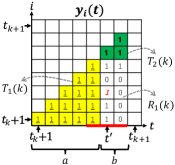
Figure 7: The updates of primal variables $z_{i}(t)$ and dual variables $y_{i}(t)$ in the $k$-th ACK interval $[t_{k}+1,t_{k+1}]$ of PDOA, where channels are OFF during $[t^{\prime}-1,t^{\prime}+1]$. The red bold italic $1$ denotes when the ACK marker equals or is larger than $1$. In addition, ${T_{1}}(k)$ is an equilateral triangle made of 1 (the underlined $1$’s with yellow background), ${T_{2}}(k)$ is an equilateral triangle made of $1$ (the bold $1$’s with green background), and ${R_{1}}(k)$ is a rectangle made of $1$ and $0$ (the regular $1$’s and $0$’s without background).

Case $2)$: The ACK marker $M$ equals or is larger than $1$ at some OFF slot $t^{\prime}$ $(t^{\prime}<t_{k+1})$ and $t_{k+1}$ is the very first ON slot after $t^{\prime}$. We use $C_{A}(k)$ to denote the total ACK cost and use $C_{H}(k)$ to denote the total holding cost in $I_{k}$. Here $P(k)=C_{A}(k)+C_{H}(k)$. We have

$${P(k)}/{D(k)} =({{C_{A}(k)+C_{H}(k)}})/{D(k)}$$ (18)

$$\buildrel(a)\over{=}{c}/{D(k)}+{C_{H}(k)}/{D(k)}$$

$$\buildrel(b)\over{\leq}{c}/{c}+{C_{H}(k)}/{D(k)}$$

$$\buildrel(c)\over{\leq}{c}/{c}+{{2\Delta D}(k)}/{D(k)}$$

$$=3,$$

where $(a)$ is because PDOA makes only one ACK at slot ${{t_{k+1}}}$ during $I_{k}$, i.e., ${C_{A}}(k)=\sum\nolimits_{t={t_{k}}+1}^{{t_{k+1}}}{c\cdot d(t)}=c\cdot d({t_{k+1}})=c$; $(b)$ is due to the dual objective value $D(k)$ is at least $c$ (i.e., when the ACK markter $M$ equals or is larger than $1$, $D(k)$ equals $c$, and $D(k)$ can be larger than $c$ due to the additional updates of the dual variables in Lines 1-1); and we prove $(c)$ as follows. The total holding cost in $I_{k}$ is

$${C_{H}}(k)$$ (19)

$$= \sum\nolimits_{\tau={t_{k}}+1}^{{t_{k+1}}}{\sum\nolimits_{i={t_{k}}+1}^{\tau}{{z_{i}}(\tau)}}$$

$$= \sum\nolimits_{\tau={t_{k}}+1}^{{t_{k+1}}-1}{\sum\nolimits_{i={t_{k}}+1}^{\tau}{{z_{i}}(\tau)}}+\sum\nolimits_{i={t_{k}}+1}^{{t_{k+1}}}{{z_{i}}({t_{k+1}})}$$

$$\buildrel(d)\over{=} \sum\nolimits_{\tau={t_{k}}+1}^{{t_{k+1}}-1}{\sum\nolimits_{i={t_{k}}+1}^{\tau}{{z_{i}}(\tau)}}+0$$

$$= \sum\nolimits_{\tau={t_{k}}+1}^{{t_{k+1}}-1}{\sum\nolimits_{i={t_{k}}+1}^{\tau}{{z_{i}}(\tau)}}$$

$$\buildrel(e)\over{=} \sum\nolimits_{\tau={t_{k}}+1}^{{t_{k+1}}-1}{\sum\nolimits_{i={t_{k}}+1}^{\tau}1}$$

$$= ({t_{k+1}}-{t_{k}}-1)({t_{k+1}}-{t_{k}})/2,$$

where in $(d)$, ${z_{i}}({t_{k+1}})=0$ for any $i\in[{t_{k}}+1,{t_{k+1}}]$ is because all the packets in $I_{k}$ are acked at slot $t_{k+1}$; and in $(e)$, ${{z_{i}}(\tau)}=1$ for any $\tau\in[{t_{k}}+1,{t_{k+1}}-1]$ and $i\in[{t_{k}}+1,\tau]$ is because the packets in $I_{k}$ are not acked until slot $t_{k+1}$, and each of them needs to pay a holding cost, i.e., ${{z_{i}}(\tau)}=1$. Similarly, the dual objective value in $I_{k}$ can be computed as $D(k)=\sum\nolimits_{\tau={t_{k}}+1}^{{t_{k+1}}-1}{\sum\nolimits_{i={t_{k}}+1}^{\tau}{{y_{i}}(\tau)}}$. We split $D(k)$ into three parts: the triangle ${T_{1}}(k)=\sum\nolimits_{\tau={t_{k}}+1}^{t^{\prime}-1}{\sum\nolimits_{i={t_{k}}+1}^{\tau}{{y_{i}}(\tau)}}$, the triangle ${T_{2}}(k)=\sum\nolimits_{\tau=t^{\prime}}^{{t_{k+1}}-1}{\sum\nolimits_{i=t^{\prime}}^{\tau}{{y_{i}}(\tau)}}$, and the rectangle ${R_{1}}(k)=\sum\nolimits_{\tau=t^{\prime}}^{{t_{k+1}}-1}{\sum\nolimits_{i={t_{k}}+1}^{t^{\prime}-1}{{y_{i}}(\tau)}}$ (see an illustration in Fig. 7). Here $D(k)={T_{1}}(k)+{T_{2}}(k)+{R_{1}}(k)$.

Our goal is to show that ${C_{H}}(k)\leq 2({T_{1}}(k)+{T_{2}}(k))\leq 2D(k)$. Here, we can compute ${T_{1}}(k)=\sum\nolimits_{\tau={t_{k}}+1}^{t^{\prime}-1}{\sum\nolimits_{i={t_{k}}+1}^{\tau}{{y_{i}}(\tau)}}=\sum\nolimits_{\tau={t_{k}}+1}^{t^{\prime}-1}{\sum\nolimits_{i={t_{k}}+1}^{\tau}1}=(t^{\prime}-{t_{k}}-1)(t^{\prime}-{t_{k}})/2$, where ${{y_{i}}(\tau)}=1$ for any $\tau\in[{t_{k}}+1,t^{\prime}-1]$ and $i\in[{t_{k}}+1,\tau]$ comes from Lines 1-1 in PDOA since the ACK marker $M$ equals or is larger than $1$ until $t^{\prime}$. In addition, we can compute ${T_{2}}(k)=\sum\nolimits_{\tau=t^{\prime}}^{{t_{k+1}}-1}{\sum\nolimits_{i=t^{\prime}}^{\tau}{{y_{i}}(\tau)}}=\sum\nolimits_{\tau=t^{\prime}}^{{t_{k+1}}-1}{\sum\nolimits_{i=t^{\prime}}^{\tau}1}=({t_{k+1}}-t^{\prime})({t_{k+1}}-t^{\prime}+1)/2$, where ${{y_{i}}(\tau)}=1$ for any $\tau\in[t^{\prime},t_{k+1}-1]$ and $i\in[t^{\prime},\tau]$ comes from Lines 1-1 in PDOA since the channels are OFF during $[t^{\prime},t_{k+1}-1]$. Let $a$ be the length of $[{t_{k}}+1,t^{\prime}-1]$ (i.e., $a=t^{\prime}-{t_{k}}-1$) and $b$ be the length of $[t^{\prime},t_{k+1}-1]$ (i.e., $b={t_{k+1}}-t^{\prime}$). Now we have ${T_{1}}(k)=a(a+1)/2$, ${T_{2}}(k)=b(b+1)/2$, and ${C_{H}}(k)=(a+b)(a+b+1)/2$. Clearly, we have

$$2D(k)-{C_{H}}(k)$$ (20)

$$=2({T_{1}}(k)+{T_{2}}(k)+{R_{1}}(k))-{C_{H}}(k)$$

$$\geq 2({T_{1}}(k)+{T_{2}}(k))-{C_{H}}(k)$$

$$=2\cdot[a(a+1)/2+b(b+1)/2]-(a+b)(a+b+1)/2$$

$$=[{(a-b)^{2}}+a+b]/2$$

$$\geq 0,$$

which completes $(c)$ in Eq. (18).

In the end, we consider the last time interval $[{t_{K}}+1,T]$ (denoted by $I_{K}$). If the last slot is an ON slot and PDOA makes the last ACK exactly at the last slot, i.e., $t_{K}=T$, then our previous analysis in Cases $1$ and $2$ still holds. Next, we consider the scenario where $t_{K}<T$. There are two cases at slot $T$: $1)$ $T$ is the slot before the ACK marker $M$ equals or is larger than $1$; $2)$ $T$ is the slot when or after the ACK marker $M$ equals or is larger than $1$. In both cases, there is no ACK made during $I_{K}$.

Case $1)$: $T$ is the slot before the ACK marker $M$ equals or is larger than $1$. In this case, the total holding cost and the total ACK cost in $I_{K}$ are $(T-{t_{K}})(T-{t_{K}}+1)/2$ and $0$, respectively. Thus, the primal objective value is $P(K)=(T-{t_{K}})(T-{t_{K}}+1)/2+0\cdot c=(T-{t_{K}})(T-{t_{K}}+1)/2$. The dual objective value is the sum of total dual variables $y_{i}(t)$ in $I_{K+1}$, which is $(T-{t_{K}})(T-{t_{K}}+1)/2$, i.e., $D(K)=(T-{t_{K}})(T-{t_{K}}+1)/2$. Therefore, we have $P(K)/D(K)=1$.

Case $2)$: $T$ is the slot when or after the ACK marker $M$ equals or is larger than $1$. We assume that the ACK marker $M$ equals or is larger than $1$ at some slot $t^{\prime}$ $(t_{K}<t^{\prime}\leq T)$. We claim that the channels are OFF during the interval $[t^{\prime},T]$. Otherwise, an ACK will be made during $[t^{\prime},T]$, which contradicts the fact that there is no ACK made during $I_{K}$. We use $C_{A}(K)$ to denote the total ACK cost and use $C_{H}(K)$ to denote the total holding cost. Here $P(K)=C_{A}(K)+C_{H}(K)=0+C_{H}(K)$, where $C_{A}(K)=0$ because there is no ACK made during $I_{K}$. We have

$${P(K)}/{D(K)} =({{C_{A}(K)+C_{H}(K)}})/{D(K)}$$ (21)

$$=0+{C_{H}(K)}/{D(K)}$$

$$\buildrel(a)\over{\leq}{{2\Delta D}(K)}/{D(K)}$$

$$=2,$$

where the analysis in $(a)$ is the same as that for $(c)$ in Eq. (18).

In summary, given any channel state $\mathbf{s}$, PDOA achieves $P(k)/D(k)\leq 3$ for any ACK interval $I_{k}$ ($k\in[0,K]$), and thus PDOA achieves $P/D\leq 3$ on the entire instance $\mathbf{s}$. By the weak duality, PDOA is 3-competitive.

-C Proof of Lemma 11

The proof outline is as follows: We first show that LAPDOA produces a feasible primal solution and an almost feasible dual solution (with a factor of $c/(c+1)$) in Lemma 5. Then, we show that in any $k$-th ACK interval, the ratio between the primal objective value and the dual objective value in this $k$-th ACK interval (denoted by $P(k)$ and $D(k)$, respectively) is at most $3/\lambda$, i.e., $P(k)/D(k)\leq 3/\lambda$. This implies that the ratio between the total primal objective value (denoted by $P$) and the total dual objective value (denoted by $D$) is also at most $3/\lambda$, i.e., $P/D\leq 3/\lambda$. Scaling down all dual variables ${y_{i}}(t)$ generated by LAPDOA by a multiplicative factor of $c/(c+1)$, we obtain a feasible dual solution with a dual objective value of $(c/(c+1))\cdot D$. By the weak duality, we have $P/OPT\leq P/((c/(c+1))\cdot D)=((c+1)/c)\cdot P/D\leq((c+1)/c)\cdot 3/\lambda$, which completes the proof.

To begin with, we introduce two key observations of LAPDOA that will be widely used in the following proofs.

Observation 3.

Assuming that LAPDOA made the latest ACK at some ON slot $L$ and the current time slot is $t$ ($t>L$), then at slot $t$, before the threshold is achieved ($M<1$), LAPDOA updates the primal variable $z_{i}(t)$ and the dual variable $y_{i}(t)$ of packet $(L+1)$ to packet $t$; however, once the threshold is achieved ($M\geq 1$) and the channel is OFF at slot $t$, LAPDOA only updates the primal variable $z_{i}(t)$ of the unacked packets.

Observation 4.

Once LAPDOA makes an ACK at some ON slot $t$, all the packets arriving no later than slot $t$ (packet $1$ to packet $t$) are acked forever after slot $t$, and their primal variables and dual variables will never be changed after slot $t$, i.e., $z_{i}(\tau)=0$ and $y_{i}(\tau)=0$ for all $i\leq t$ and all $\tau\geq t$.

Then, we show that LAPDOA gives an almost feasible solution in Lemma 5.

Lemma 5.

LAPDOA produces a feasible solution to primal Problem (6). In addition, let $\mathbf{y}\triangleq\{\{{y_{i}}(t)\}_{i=1}^{t}\}_{t=1}^{T}$ be the solution produced by LAPDOA to dual Problem (7), then $(c/(c+1))\mathbf{y}$ is a feasible solution to dual Problem (7).

Proof.

We omit the proof for primal constraints (6b)-(6c) and dual constraint (7c) because they are similar to the proof in Lemma 4 and provide the proof for dual constraint (7b). Consider an ON slot $t$ and its dual constraint (7b) $\sum_{i=1}^{t}\sum_{\tau=t}^{T}y_{i}(\tau)\leq c$. Recall that this dual constraint requires that for all the packets arriving no later than slot $t$, the sum of their dual variables beyond slot $t$ should not exceed $c$. We assume that this ON slot $t$ falls into the $k$-th ACK interval $[t_{k}+1,t_{k+1}]$, i.e., ${t_{k}}+1\leq t\leq{t_{k+1}}$, where LAPDOA makes two ACKs at the ON slots $t_{k}$ and $t_{k+1}$ (in a special case that the ON slot $t$ falls into the last interval $[t_{K}+1,T]$, i.e., ${t_{K}}+1\leq t\leq T$, where LAPDOA makes the last ACK at the ON slot $t_{K}$, our following analysis can be extended to this case). According to Observations 3 and 4, packet $1$ to packet $t_{k}$ are not updated after slot $t_{k}$, and packet $(t_{k}+1)$ to packet $t$ are not updated after slot $t_{k+1}$, similar to Eq. (15), we have $\sum_{i={1}}^{t}\sum_{\tau=t}^{T}y_{i}(\tau)=\sum_{i={t_{k}}+1}^{t}\sum_{\tau=t}^{{{t_{k+1}}}}y_{i}(\tau)$. Furthermore, we assume that during the interval $[t,{t_{k+1}}]$, all packets arriving between $[t_{k}+1,t]$ (packet $t_{k}+1$ to packet $t$) make $m$ big updates and $n$ small updates (some zero updates can also be made but we ignore them since they cannot increase the dual variables). In other words, we have $\sum_{i={t_{k}}+1}^{t}\sum_{\tau=t}^{{{t_{k+1}}}}y_{i}(\tau)=1\cdot m+\lambda\cdot n=m+\lambda n$. We claim that if $m+\lambda n\geq c$, then the increment of ACK marker $M$ due to those $m$ big and $n$ small updates (denoted by $M(m,n)$) will be larger than or equal to $1$. This is true since we have $M(m,n)=m\cdot(1/\lambda c)+n\cdot(\lambda/c)=m/\lambda c+\lambda n/c\geq m/c+\lambda n/c=(m+\lambda n)/c\geq c/c=1$. This claim, in turn, implies that $\sum_{i={t_{k}}+1}^{t}\sum_{\tau=t}^{{{t_{k+1}}}}y_{i}(\tau)=m+\lambda n<c+1$. To see this, consider the edge case where there are $m^{\prime}$ big updates and $n^{\prime}$ small updates made by all packets arriving between $[t_{k}+1,t]$ since slot $t$, and they satisfy: (i) their sum of dual variables is smaller than $c$, i.e., $m^{\prime}+\lambda n^{\prime}<c$; (ii) with one more update (either big or small), the sum of their dual variables is no less than $c$, i.e., either $(m^{\prime}+1)+\lambda n^{\prime}\geq c$ or $m^{\prime}+\lambda(n^{\prime}+1)\geq c$ holds. From condition (ii) and our claim we know that with the arrival of one more update, the ACK marker $M$ will be larger than or equal to be $1$ (because we have $M\geq M(m,n)\geq 1$) at some slot $t^{\prime}$ ($t^{\prime}\leq t_{k+1}$). When this happens, the sum of dual variables is at most $\max\{(m^{\prime}+1)+\lambda n^{\prime},m^{\prime}+\lambda(n^{\prime}+1)\}=(m^{\prime}+1)+\lambda n^{\prime}=(m^{\prime}+\lambda n^{\prime})+1<c+1$, and those dual variables will never be updated after slot $t^{\prime}$ according to Observation 3. Therefore, we have $\sum_{i={1}}^{t}\sum_{\tau=t}^{T}y_{i}(\tau)=\sum_{i={t_{k}}+1}^{t}\sum_{\tau=t}^{{{t_{k+1}}}}y_{i}(\tau)<c+1$. Now scaling down the dual solution $\bf{y}$ by a factor of $c/(c+1)$, we obtain a feasible dual solution $(c/(c+1))\mathbf{y}$. ∎

In the following, we assume that $d(t)$ is updated to the ACK marker $M$ $(M\geq 1)$ rather than $1$ in Line 2, which possibly makes LAPDOA perform worse (i.e., has a larger total cost since the one-time ACK cost now is $c\cdot M$, which is larger than or equal to $c\cdot 1$). We show that our CR analysis holds for this worse setting (i.e., $d(t)=M$), and thus our CR analysis also holds for LAPDOA. The benefit of considering this worse setting is that this allows us to allocate the ACK costs to large and small updates. Specifically, under the worse setting, suppose that LAPDOA makes an ACK at slot $t_{k}$, and after $m$ ($m\geq 0$) big updates and $n$ ($n\geq 0$) small updates, LAPDOA is ready to make another ACK at some slot $t_{k+1}$. At this point, the ACK marker is $M=m/(\lambda c)+n\lambda/c$, and the ACK cost is $c\cdot M=m/\lambda+n\lambda$. However, instead of calculating the ACK cost at slot $t_{k+1}$, we can distribute the ACK cost to the updates in $[t_{k}+1,t_{k+1}]$, that is, each big update gets an ACK cost of $1/\lambda$ and each small update gets an ACK cost of $\lambda$. The total ACK cost of those $m$ big updates and $n$ small updates is still $m/\lambda+n\lambda$. Doing this does not change the ACK cost, but now every big update or small update has a contribution to the ACK cost, which helps our analysis in the following when we compute the primal increment (i.e., the sum of ACK cost and holding cost) of each update.

We assume that LAPDOA makes a sequence of ACKs $\pi=\{t_{1},t_{2},\dots,t_{K}\}$, where LAPDOA makes the $i$-th ACK at the ON slot $t_{i}$ (i.e., $s(t_{i})d(t_{i})=1$). Our goal is to show that for any $k$-th ($k\in[0,K]$) ACK interval $[{t_{k}}+1,{t_{k+1}}]$ (where the first ACK interval is $[1,{t_{1}}]$ when $k=0$ and the last ACK interval is $[{t_{K}}+1,T]$ when $k=K$), the ratio between the primal objective value and the dual objective value in this $k$-th ACK interval is at most $3$, i.e., $P(k)/D(k)\leq 3/\lambda$. According to Observation 4, when this ACK interval ends at slot $t_{k+1}$, $P(k)$ and $D(k)$ are never changed. This implies that LAPDOA also achieves $P/{D}\leq 3/\lambda$ on the entire instance $\mathbf{s}$.

We first discuss the relation between $P(k)$ and $D(k)$ in the first $K$ ACK interval $[{t_{k}}+1,{t_{k+1}}]$ (i.e., $k\in[0,K-1]$, where there is always an ACK made at slot $t_{k+1}$), and then discuss the relation between $P(K)$ and $D(K)$ in the last ACK interval $[{t_{K}}+1,T]$ (i.e., $k=K$, where it is possible that no ACK is made at slot $T$) in the end.

Consider the $k$-th ($k\in[0,K-1]$) ACK interval $[{t_{k}}+1,{t_{k+1}}]$ (denoted by $I_{k}$), where LAPDOA makes two ACKs at the ON slots $t_{k}$ and $t_{k+1}$ (the first ACK interval is the $0$-th ACK interval $[{t_{0}}+1,{t_{1}}]$, where $t_{0}=0$ and LAPDOA only makes one ACK at slot $t_{1}$), respectively. There are two cases when we make an ACK at slot $t_{k+1}$: $1)$ the ACK marker $M$ is equal to or larger than $1$ at $t_{k+1}$; $2)$ the ACK marker $M$ equals or is larger than $1$ at some OFF slot $t^{\prime}$ $(t^{\prime}<t_{k+1})$ and $t_{k+1}$ is the very first ON slot after slot $t^{\prime}$ (in this case, the channels are OFF during $[t^{\prime},t_{k+1}-1]$). We analyze the performance of LAPDOA in these two cases of $t_{k+1}$.

Case $1)$: The ACK marker $M$ is equal to or larger than $1$ at $t_{k+1}$. In this case, we do not have zero updates in $I_{k}$. Let $\Delta P$ and $\Delta D$ denote the increment of the primal objective value and the increment of the dual objective value when we make an update, respectively. In the case of a small update, we have $\Delta P=\lambda+1$ and $\Delta D=\lambda$, that is, $\Delta P/\Delta D=1+1/\lambda$. In the case of a big update, $\Delta P=1/\lambda+1$ and $\Delta D=1$, and we still have $\Delta P/\Delta D=1+1/\lambda$. Obviously, for this $k$-th ACK interval, we have $P(k)/D(k)=1+1/\lambda$.

Case $2)$: The ACK marker $M$ equals or is larger than $1$ at some OFF slot $t^{\prime}$ $(t^{\prime}<t_{k+1})$ and $t_{k+1}$ is the very first ON slot after slot $t^{\prime}$. An illustration is shown in Fig. 2. We use $C_{A}(k)$ and $C_{H}(k)$ to denote the ACK costs and holding costs in $I_{k}$, respectively. Here $P(k)=C_{A}(k)+C_{H}(k)$. In addition, we assume that there are $m$ ($m\geq 0$) big updates and $n$ ($n\geq 0$) small updates in $I_{k}$ (some zero updates can also be made but we ignore them since they cannot increase the ACK cost and the dual variable). Given that each big update has an ACK cost of $1/\lambda$ and increases the dual variable by $1$, and each small update has an ACK cost of $\lambda$ and increases the dual variable by $\lambda$, we have ${C_{A}}(k)=m/\lambda+\lambda n$ and $D(k)\geq m+\lambda n$ (i.e., $D(k)$ can be larger than $m+\lambda n$ due to the additional updates of dual variables in Lines 2-2).

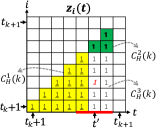
(a) Primal variables $z_{i}(t)$ updates.

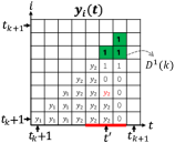
(b) Dual variables $y_{i}(t)$ updates.

Figure 8: An illustration of $C_{H}^{1}(k),C_{H}^{2}(k),C_{H}^{3}(k)$ and ${D^{1}}(k)$ when $j\neq t^{\prime}$. $C_{H}^{1}(k)$ is an equilateral triangle made of 1 (the underlined $1$’s with yellow background in Fig. 8(a)), $C_{H}^{2}(k)$ is an equilateral triangle made of $1$ (the bold $1$’s with green background in Fig. 8(a)), $C_{H}^{3}(k)$ is a rectangle made of $1$ (the regular $1$’s without background in Fig. 8(a)), and ${D^{1}}(k)$ is an equilateral triangle made of 1 (the bold $1$’s with green background in Fig. 8(b)).

Now we can compute

$$P(k)/D(k)$$ (22)

$$=({C_{A}(k)+C_{H}(k)})/{D(k)}$$

$$=(m/\lambda+\lambda n+C_{H}(k))/{D(k)}$$

$$\leq(m/\lambda+\lambda n)/({m+\lambda n})+C_{H}(k)/{D(k)}$$

$$\leq 1/{\lambda}+C_{H}(k)/D(k)$$

$$\buildrel(a)\over{\leq}1/\lambda+2/\lambda$$

$$=3/\lambda,$$

where $(a)$ is proven in the following. Similar to the analysis of Case-$(2)$ in the proof of Theorem 1, we can first compute the total holding cost in $I_{k}$ as ${C_{H}}(k)=\sum\nolimits_{\tau={t_{k}}+1}^{{t_{k+1}}-1}{\sum\nolimits_{i={t_{k}}+1}^{\tau}{{z_{i}}(\tau)}}=\sum\nolimits_{\tau={t_{k}}+1}^{{t_{k+1}}-1}{\sum\nolimits_{i={t_{k}}+1}^{\tau}1}=({t_{k+1}}-{t_{k}}-1)({t_{k+1}}-{t_{k}})/2$, where ${{z_{i}}(\tau)}=1$ for any $\tau\in[{t_{k}}+1,{t_{k+1}}-1]$ and $i\in[{t_{k}}+1,\tau]$ is because the packets in $I_{k}$ are not acked until slot $t_{k+1}$, and they need to pay a holding cost, i.e., ${{z_{i}}(\tau)}=1$. Next, we split ${C_{H}}(k)$ into three parts under two different cases. Assuming that the ACK marker $M$ is equal to or larger than $1$ after the updating of $j$-th packet at slot $t^{\prime}$. There are two cases for packet $j$: $1)$ packet $j$ is not packet $t^{\prime}$ ($j\neq t^{\prime}$), and $2)$ packet $j$ is packet $t^{\prime}$ ($j=t^{\prime}$). In the first case ($j\neq t^{\prime}$), we can split ${C_{H}}(k)$ into $C_{H}^{1}(k)=\sum\nolimits_{\tau={t_{k}}+1}^{t^{\prime}-1}{\sum\nolimits_{i={t_{k}}+1}^{\tau}{{z_{i}}(\tau)}}$, $C_{H}^{2}(k)=\sum\nolimits_{\tau=t^{\prime}}^{{t_{k+1}}-1}{\sum\nolimits_{i=t^{\prime}}^{\tau}{{z_{i}}(\tau)}}$, and $C_{H}^{3}(k)=\sum\nolimits_{\tau=t^{\prime}}^{{t_{k+1}}-1}{\sum\nolimits_{i={t_{k}}+1}^{t^{\prime}-1}{{z_{i}}(\tau)}}$ (see an illustration in Fig. 8). In addition, when $j\neq t^{\prime}$, we know that the total number of big updates and small updates satisfies $m+n=\sum\nolimits_{\tau={t_{k}}+1}^{t^{\prime}-1}{\sum\nolimits_{i={t_{k}}+1}^{\tau}{{z_{i}}(\tau)}+}\sum\nolimits_{i={t_{k}}+1}^{j}{{z_{i}}(t^{\prime})}\geq\sum\nolimits_{\tau={t_{k}}+1}^{t^{\prime}-1}{\sum\nolimits_{i={t_{k}}+1}^{\tau}{{z_{i}}(\tau)}=}C_{H}^{1}(k)$.

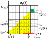
(a) Primal variables $z_{i}(t)$ updates.

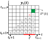
(b) Dual variables $y_{i}(t)$ updates.

Figure 9: An illustration of $C_{H}^{1}(k),C_{H}^{2}(k),C_{H}^{3}(k)$ and ${D^{1}}(k)$ when $j=t^{\prime}$. $C_{H}^{1}(k)$ is an equilateral triangle made of 1 (the underlined $1$’s with yellow background in Fig. 9(a)), $C_{H}^{2}(k)$ is an equilateral triangle made of $1$ (the bold $1$’s with green background in Fig. 9(a)), $C_{H}^{3}(k)$ is a rectangle made of $1$ (the regular $1$’s without background in Fig. 9(a)), and ${D^{1}}(k)$ is an equilateral triangle made of 1 (the bold $1$’s with green background in Fig. 9(b)).

In the second case ($j=t^{\prime}$), we can split ${C_{H}}(k)$ into $C_{H}^{1}(k)=\sum\nolimits_{\tau={t_{k}}+1}^{t^{\prime}}{\sum\nolimits_{i={t_{k}}+1}^{\tau}{{z_{i}}(\tau)}}$, $C_{H}^{2}(k)=\sum\nolimits_{\tau=t^{\prime}+1}^{{t_{k+1}}-1}{\sum\nolimits_{i=t^{\prime}+1}^{\tau}{{z_{i}}(\tau)}}$, and $C_{H}^{3}(k)=\sum\nolimits_{\tau=t^{\prime}+1}^{{t_{k+1}}-1}{\sum\nolimits_{i={t_{k}}+1}^{t^{\prime}}{{z_{i}}(\tau)}}$ (see an illustration in Fig. 9). Furthermore, when $j=t^{\prime}$, we know that the total number of big updates and small updates satisfies $m+n=\sum\nolimits_{\tau={t_{k}}+1}^{t^{\prime}}{\sum\nolimits_{i={t_{k}}+1}^{\tau}{{z_{i}}(\tau)}}=C_{H}^{1}(k)$. In the following, we only focus on the analysis of $D(k)$ in the first case since the analysis in the second case is very similar. According to Lines 2-2, for the dual variables, we have an equilateral triangle made of $1$, which has the same shape as $C_{H}^{2}(k)$, we denote it by ${D^{1}}(k)$ (see an illustration in Fig. 8). We can calculate that ${D^{1}}(k)=\sum\nolimits_{\tau=t^{\prime}}^{{t_{k+1}}-1}{\sum\nolimits_{i=t^{\prime}}^{\tau}{{y_{i}}(\tau)}}=\sum\nolimits_{\tau=t^{\prime}}^{{t_{k+1}}-1}{\sum\nolimits_{i=t^{\prime}}^{\tau}1}=C_{H}^{2}(k)$. Now we can compute

$$C_{H}(k) =C_{H}^{1}(k)+C_{H}^{2}(k)+C_{H}^{3}(k)$$ (23)

$$\buildrel(a)\over{\leq}2(C_{H}^{1}(k)+C_{H}^{2}(k))$$

$$\buildrel(b)\over{\leq}2((m+n)+C_{H}^{2}(k))$$

$$\buildrel\over{=}2((m+n)+{D^{1}}(k))$$

$$\leq 2(({m+\lambda n})/{\lambda}+({{D^{1}}(k)})/{\lambda})$$

$$=2/\lambda\cdot(m+\lambda n+{D^{1}}(k))$$

$$\buildrel(c)\over{\leq}2/\lambda\cdot D(k),$$

where $(a)$ can be proven using the same techniques in Eq. (20), $(b)$ is because $C_{H}^{1}(k)$ is at least $m+n$ as we analyzed above, and $(c)$ is because $D(k)$ is least $m+\lambda n+{D^{1}}(k)$ (i.e., $D(k)$ can be larger than $m+\lambda n+{D^{1}}(k)$ due to Lines 2-2). This completes (a) in Eq. (22).

In the end, we consider the last time interval $[{t_{K}}+1,T]$ (denoted by $I_{K}$). If the last slot is an ON slot and LAPDOA makes the last ACK exactly at the last slot, i.e., $t_{K}=T$, then our previous analysis in Cases $1$ and $2$ still holds. Next, we consider the scenario where $t_{K}<T$. There are two cases at slot $T$: $1)$ $T$ is the slot before the ACK marker $M$ equals or is larger than $1$; $2)$ $T$ is the slot when or after the ACK marker $M$ equals or is larger than $1$. In both cases, there is no ACK made during $I_{K}$. We use $P(K)$ and $D(K)$ to denote the primal objective value and the dual objective value in $I_{K}$, respectively.

Case $1)$: $T$ is the slot before the ACK marker $M$ equals or is larger than $1$. In this case, we do not have zero updates in $I_{K}$. Let $\Delta P$ and $\Delta D$ denote the increment of the primal objective value and the increment of the dual objective value when we make an update, respectively. In the case of a small update, we have $\Delta P=c\cdot 0+1=1$ and $\Delta D=\lambda$, that is, $\Delta P/\Delta D=1/\lambda$. In the case of a big update, $\Delta P=c\cdot 0+1=1$ and $\Delta D=1$, so we have $\Delta P/\Delta D=1$. Obviously, for this $K$-th ACK interval, we have $P(K)/D(K)\leq 1/\lambda$.

Case $2)$: $T$ is the slot when or after the ACK marker $M$ equals or is larger than $1$. We assume that the ACK marker $M$ equals or is larger than $1$ at slot $t^{\prime}$ $(t^{\prime}>t_{K})$. According to the definition of Case $2$, we have $T\geq t^{\prime}$. We claim that the channels are OFF during the interval $[t^{\prime},T]$. Otherwise, an ACK will be made during $[t^{\prime},T]$, which contradicts the fact that there is no ACK during $I_{K}$. We use $C_{A}(K)$ to denote the total ACK cost and use $C_{H}(K)$ to denote the total holding cost in $I_{K}$. Here $P(K)=C_{A}(K)+C_{H}(K)=0+C_{H}(K)$, where $C_{A}(K)=0$ because there is no ACK made during $I_{K}$. We have

$${P(K)}/{D(K)} =({{C_{A}(K)+C_{H}(K)}})/{D(K)}$$ (24)

$$=0+{C_{H}(K)}/{D(K)}$$

$$\buildrel(a)\over{\leq}2/\lambda,$$

where the analysis in $(a)$ is the same as the (a) in Eq. (22).

In summary, LAPDOA achieves $P(k)/{D}(k)\leq 3/\lambda$ for any ACK interval, and thus LAPDOA also achieves $P/{D}\leq 3/\lambda$ on the entire instance.

-D Proof of Lemma 3

Proof.

In this proof, similar to the proof of Lemma 11, we still assume that $d(t)$ is updated to the ACK marker $M$ $(M\geq 1)$ rather than $1$ in Line 2 (except the analysis of big updates in the case of $\lambda\in(0,1/c]$, where we still update $d(t)$ to be $1$). Therefore, for the big updates and small updates in any ACK interval, each big update can be charged with an ACK cost of $1/\lambda$, and each small update can be charged with an ACK cost of $\lambda$. In particular, for the big updates and small updates in the last time interval $[t_{K},T]$ (we assume that LAPDOA makes the last ACK at slot $t_{K}$), though there is no ACK made during $[t_{K},T]$, we still charge each big update and each small update with an ACK cost of $1/\lambda$ and $\lambda$, respectively. Doing this can possibly increase the total cost of LAPDOA, but we can show that the upper bound we derived still holds in this case.

We first consider $\lambda\in(0,1/c]$. In this case, LAPDOA has three types of updates: big updates, small updates, and zero updates. Consider the total cost of big updates first. Once the prediction $\mathcal{P}$ makes an ACK at some ON slot $t$, LAPDOA will make a big update immediately, the ACK marker becomes $M=1/\lambda c=1/c\cdot 1/\lambda\geq 1/c\cdot c=1$, and thus LAPDOA will also make an ACK at the beginning of slot $t$. Since the prediction $\mathcal{P}$ has a total number of $C_{A}(\mathbf{s},\mathcal{P})/c$ ACKs, then LAPDOA has also $C_{A}(\mathbf{s},\mathcal{P})/c$ big updates. Each big update leads to an ACK, which results in an ACK cost of $c$. Therefore, the total cost of the big updates in LAPDOA is $C_{A}(\mathbf{s},\mathcal{P})/c\cdot c=C_{A}(\mathbf{s},\mathcal{P})$. By the definition of small update and zero update, each small update or zero update in LAPDOA corresponds to one packet in the prediction $\mathcal{P}$ that has not been acked yet, which requires the prediction $\mathcal{P}$ to pay a holding cost of $1$, so the total number of small updates and zero udpates is at most $C_{H}(\mathbf{s},\mathcal{P})/1=C_{H}(\mathbf{s},\mathcal{P})$. For each of the small updates, the increase in the primal is $\Delta P=\lambda+1$, and for each of the zero updates, the increase in the primal is $\Delta P=0+1=1$, so the total cost of small updates and zero updates is at most $(1+\lambda)C_{H}(\mathbf{s},\mathcal{P})$. This concludes Eq. (12).

Next, we analyze $\lambda\in(1/c,1]$. We consider two cases: $1)$ the channels are ON all the time, and $2)$ there are some OFF channels. We show that Eq. (13) holds for both cases.

Case $1)$: The channels are ON all the time. In this case, LAPDOA will generate only two types of updates: small updates and big updates. By the definition of small updates, for any of them, there is one corresponding packet in the prediction $\mathcal{P}$ that has not been acked yet, which requires the prediction $\mathcal{P}$ to pay a holding cost of $1$ for this packet, so the total number of the small updates is at most $C_{H}(\mathbf{s},\mathcal{P})/1=C_{H}(\mathbf{s},\mathcal{P})$. Each small update contributes $(\lambda+1)$ to the primal objective value, thus the total cost of small updates is at most $(1+\lambda)C_{H}(\mathbf{s},\mathcal{P})$. Next, we analyze the total cost of big updates. We claim that for any ACK made by the prediction $\mathcal{P}$, LAPDOA makes at most $\left\lceil{\lambda c}\right\rceil$ big updates for this ACK. To see this, assuming that prediction $\mathcal{P}$ makes an ACK at slot $t$, and consider all the big updates due to this ACK (i.e., those big updates produced by the packets in LAPDOA that have not been acked yet and arrives before or at slot $t$). After at most $\left\lceil{\lambda c}\right\rceil$ such big updates, the ACK marker will become $M=\left\lceil{\lambda c}\right\rceil\cdot 1/\lambda c\geq 1$ at some slot $t^{\prime}\geq t$. Once the ACK marker $M$ equals or is larger than $1$, no more big updates will be made for the ACK made by prediction $\mathcal{P}$ at slot $t$. Given that prediction $\mathcal{P}$ makes $C_{A}(\mathbf{s},\mathcal{P})/c$ ACKs, then LAPDOA makes at most $\left\lceil{\lambda c}\right\rceil\cdot C_{A}(\mathbf{s},\mathcal{P})/c$ big updates. For each big update, the increment in the primal objective value is $\Delta P=1/\lambda+1$. Therefore, the total cost of big updates is at most $(1/\lambda+1)\cdot\left\lceil{\lambda c}\right\rceil\cdot C_{A}(\mathbf{s},\mathcal{P})/c$. In summary, when the channels are always ON, the total cost of LAPDOA is upper bounded by $C(\mathbf{s},\mathcal{P},\lambda)\leq(\lambda+1)C_{H}(\mathbf{s},\mathcal{P})+(1/\lambda+1)\left\lceil{\lambda c}\right\rceil{C_{A}(\mathbf{s},\mathcal{P})}/{c},$ which is smaller than the bound in Eq. (13).

Case $2)$: There are some OFF channels. In this case, LAPDOA will generate three types of updates: small updates, big updates, and zero updates. Note that these zero updates only increase the holding costs. We use ${C_{A,s}}$ and ${C_{H,s}}$ to denote the ACK cost and the holding cost of all the small updates, respectively; use ${C_{A,b}}$ and ${C_{H,b}}$ to denote the ACK cost and the holding cost of all the big updates, respectively; and ${C_{H,z}}$ to denote the holding cost of all the zero updates. Obviously, we have $C({\bf{s}},{\cal P},\lambda)={C_{A,b}}+{C_{H,b}}+{C_{A,s}}+{C_{H,s}}+{C_{H,z}}$. Furthermore, similar to the analysis in Case $1$, for the big updates, we can obtain ${C_{A,b}}+{C_{H,b}}\leq(1/\lambda+1)\cdot\left\lceil{\lambda c}\right\rceil\cdot{C_{A}}({\bf{s}},{\cal P})/c$; and for the small updates, we have ${C_{A,s}}+{C_{H,s}}\leq(\lambda+1){C_{H}}({\bf{s}},{\cal P})$. To analyze the holding costs of zero updates ${C_{H,z}}$, our idea is to bound it by the holding cost of small updates and big updates, which can be further bounded by the total cost of prediction. To this end, we assume that LAPDOA makes a sequence of ACKs $\pi=\{t_{1},t_{2},\dots,t_{K}\}$, where LAPDOA makes the $i$-th ACK at the ON slot $t_{i}$ (i.e., $s(t_{i})d(t_{i})=1$). Our goal is to show that in any $k$-th ($k\in[0,K]$) ACK interval $[{t_{k}}+1,{t_{k+1}}]$ (where the first ACK interval is $[1,{t_{1}}]$ when $k=0$ and the last ACK interval is $[{t_{K}}+1,T]$ when $k=K$), the holding costs of zero updates can be bounded by the holding cost of small updates and big updates.

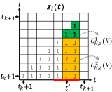
(a) when $j\neq t^{\prime}$

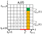
(b) when $j=t^{\prime}$

Figure 10: An illustration of $C_{H,z}(k)$, $C_{H,z}^{1}(k)$, and $C_{H,z}^{2}(k)$ in two different cases ($j\neq t^{\prime}$ and $j=t^{\prime}$). $C_{H,z}(k)$ is the sum of the underlined $1$’s, $C_{H,z}^{1}(k)$ is an equilateral triangle made of $1$ (the bold underlined $1$’s with green background), and $C_{H,z}^{2}(k)$ is a rectangle made of $1$ (the sum of some regular $1$’s and some underlined $1$’s with orange background).

We consider the $k$-th ($k\in[0,K-1]$) ACK interval $[{t_{k}}+1,{t_{k+1}}]$ (denoted by $I_{k}$), where the LAPDOA makes two ACKs at the ON slots $t_{k}$ and $t_{k+1}$, respectively. Still, there are two cases when we make an ACK at $t_{k+1}$: $1)$ the ACK marker $M$ is equal to or larger than $1$ at $t_{k+1}$ and $t_{k+1}$ is an ON slot; $2)$ the ACK marker $M$ equals or is larger than $1$ at some OFF slot $t^{\prime}$ $(t^{\prime}<t_{k+1})$ and $t_{k+1}$ is the very first ON slot after slot $t^{\prime}$. Note that though the following analysis is for the general ACK interval $[{t_{k}}+1,{t_{k+1}}]$ ($k\in[0,K-1]$), they can be easily extended the last ACK interval $[{t_{K}}+1,T]$.

1. The ACK marker $M$ is equal to or larger than $1$ at the ON slot $t_{k+1}$. In this case, there is no zero update, and the holding cost of zero updates is $0$.

2. The ACK marker $M$ equals or is larger than $1$ at some OFF slot $t^{\prime}$ $(t^{\prime}<t_{k+1})$ and $t_{k+1}$ is the very first ON slot after slot $t^{\prime}$ (i.e., the channels are OFF during $[t^{\prime},t_{k+1}-1]$). Assuming that the ACK marker $M$ is equal to or larger than $1$ after the updating of the $j$-th packet at slot $t^{\prime}$. In this case, for the holding costs of zero updates in $I_{k}$ (denoted by ${C_{H,z}}(k)$), we can compute it under two different cases based on packet $j$: $1)$ packet $j$ is not packet $t^{\prime}$ ($j\neq t^{\prime}$), and $2)$ packet $j$ is packet $t^{\prime}$ ($j=t^{\prime}$). In the first case ($j\neq t^{\prime}$), we can denote ${C_{H,z}}(k)$ as ${C_{H,z}}(k)=\sum\nolimits_{i=j+1}^{t^{\prime}}{{z_{i}}(t^{\prime})}+\sum\nolimits_{\tau=t^{\prime}+1}^{{t_{k+1}}-1}{\sum\nolimits_{i={t_{k}}+1}^{\tau}{{z_{i}}(\tau)}}$ (see an illustration in Fig. 10(a)); and in the second case ($j=t^{\prime}$), we can denote ${C_{H,z}}(k)$ as ${C_{H,z}}(k)=\sum\nolimits_{\tau=t^{\prime}+1}^{{t_{k+1}}-1}{\sum\nolimits_{i={t_{k}}+1}^{\tau}{{z_{i}}(\tau)}}$ (see an illustration in Fig. 10(b)). In the following, we only focus on the analysis of ${C_{H,z}}(k)$ in the first case since the analysis in the second case is very similar. Next, we bound ${C_{H,z}}(k)$ by two areas: $C_{H,z}^{1}(k)\triangleq\sum\nolimits_{\tau=t^{\prime}}^{{t_{k+1}}-1}{\sum\nolimits_{i=t^{\prime}}^{\tau}{{z_{i}}(\tau)}}$ and $C_{H,z}^{2}(k)\triangleq\sum\nolimits_{\tau=t^{\prime}}^{{t_{k+1}}-1}{\sum\nolimits_{i={t_{k}}+1}^{t^{\prime}-1}{{z_{i}}(\tau)}}$ (see an illustration in Fig. 10(a)). Clearly, we have ${C_{H,z}}(k)=\sum\nolimits_{i=j+1}^{t^{\prime}}{{z_{i}}(t^{\prime})}+\sum\nolimits_{\tau=t^{\prime}+1}^{{t_{k+1}}-1}{\sum\nolimits_{i={t_{k}}+1}^{\tau}{{z_{i}}(\tau)}}\leq\sum\nolimits_{\tau=t^{\prime}}^{{t_{k+1}}-1}{\sum\nolimits_{i=t^{\prime}}^{\tau}{{z_{i}}(\tau)}}+\sum\nolimits_{\tau=t^{\prime}}^{{t_{k+1}}-1}{\sum\nolimits_{i={t_{k}}+1}^{t^{\prime}-1}{{z_{i}}(\tau)}}=C_{H,z}^{1}(k)+C_{H,z}^{2}(k)$. We use $C_{H,z}^{1}$ to denote the sum of $C_{H,z}^{1}(k)$ over all the ACK intervals $I_{k}$ ($k\in[0,K]$), i.e., $C_{H,z}^{1}\triangleq\sum\nolimits_{k=0}^{K}{C_{H,z}^{1}(k)}$. For any of the zero updates in $C_{H,z}^{1}$, there is one corresponding packet in the prediction $\mathcal{P}$ that has not been acked yet since the channels are OFF during some $[t^{\prime},{t_{k+1}}-1]$, which requires the prediction $\mathcal{P}$ to pay a holding cost of $1$ for this packet. Similarly, for any of the small updates, by the definition of small updates, there is one corresponding packet in the prediction $\mathcal{P}$ that has not been acked yet, which requires the prediction $\mathcal{P}$ to pay a holding cost of $1$ for this packet. Therefore, the total number of the zero updates in $C_{H,z}^{1}$ and the small updates is at most $C_{H}(\mathbf{s},\mathcal{P})/1=C_{H}(\mathbf{s},\mathcal{P})$, and each of such update has a total cost at most $(1+\lambda)$, which indicates that the total cost of the zero updates in $C_{H,z}^{1}$ and the small updates is at most $(1+\lambda)C_{H}(\mathbf{s},\mathcal{P})$, i.e.,

   $${C_{A,s}}+{C_{H,s}}+C_{H,z}^{1}\leq(1+\lambda)C_{H}(\mathbf{s},\mathcal{P}).$$ (25)

   For the holding cost $C_{H,z}^{2}(k)$, same as the analysis in $(a)$ of Eq. (23), it is upper bounded by the sum of the holding cost of big updates and small updates in $I_{k}$ and the holding cost of the zero updates in $C_{H,z}^{1}(k)$, i.e., $C_{H,z}^{2}(k)\leq C_{H,s}(k)+C_{H,b}(k)+C_{H,z}^{1}(k)$. More generally, let $C_{H,z}^{2}$ denote the sum of $C_{H,z}^{2}(k)$ over all the ACK intervals $I_{k}$ ($k\in[0,K]$), i.e., $C_{H,z}^{2}\triangleq\sum\nolimits_{k=0}^{K}{C_{H,z}^{2}(k)}$. Then we have

   $$C_{H,z}^{2} \leq C_{H,s}+C_{H,b}+C_{H,z}^{1}$$

   $$=(C_{H,s}+C_{H,z}^{1})+C_{H,b}$$

   $$\buildrel(a)\over{\leq}C_{H}(\mathbf{s},\mathcal{P})+C_{H,b}$$

   $$\buildrel(b)\over{\leq}C_{H}(\mathbf{s},\mathcal{P})+\left\lceil{\lambda c}\right\rceil\times{C_{A}(\mathbf{s},\mathcal{P})}/{c},$$

   where $(a)$ is because as we showed before, the total number of the zero updates in $C_{H,z}^{1}$ and the small updates is at most $C_{H}(\mathbf{s},\mathcal{P})$, and each of small updates or zero updates increases the holding costs of LAPDOA by $1$, so the total holding cost of them is at most $C_{H}(\mathbf{s},\mathcal{P})$; $(b)$ is due to the total number of big updates is at most $\left\lceil{\lambda c}\right\rceil\times C_{A}(\mathbf{s},\mathcal{P})/c$, and each of big updates increases the holding costs by $1$, so we have $C_{H,b}\leq\left\lceil{\lambda c}\right\rceil\times C_{A}(\mathbf{s},\mathcal{P})/c$.

In summary, the total cost of LAPDOA in Case $2$ is

$$C(\mathbf{s},\mathcal{P},\lambda)$$

$$={C_{A,b}}+{C_{H,b}}+{C_{A,s}}+{C_{H,s}}+{C_{H,z}}$$

$$\leq{C_{A,b}}+{C_{H,b}}+{C_{A,s}}+{C_{H,s}}+C_{H,z}^{1}+C_{H,z}^{2}$$

$$=({C_{A,b}}+{C_{H,b}})+({C_{A,s}}+{C_{H,s}}+C_{H,z}^{1})+C_{H,z}^{2}$$

$$\leq(1/\lambda+1)\times\left\lceil{\lambda c}\right\rceil\times{C_{A}(\mathbf{s},\mathcal{P})}/{c}+(1+\lambda)C_{H}(\mathbf{s},\mathcal{P})$$

$$\quad+C_{H}(\mathbf{s},\mathcal{P})+\left\lceil{\lambda c}\right\rceil\times{C_{A}(\mathbf{s},\mathcal{P})}/{c}$$

$$=(1/\lambda+2)\times\left\lceil{\lambda c}\right\rceil\times{C_{A}(\mathbf{s},\mathcal{P})}/{c}+(2+\lambda)C_{H}(\mathbf{s},\mathcal{P}).$$

Finally, combining the results in Case $1$ and Case $2$, we see that Eq. (13) holds. ∎

References

- [1] Z. Liu, K. Zhang, B. Li, Y. Sun, T. Hou, and B. Ji, “Learning-augmented online minimization of age of information and transmission costs,” in IEEE INFOCOM WKSHPS: ASoI 2024: IEEE INFOCOM Age and Semantics of Information Workshop (INFOCOM ASoI 2024), Vancouver, Canada, May 2024, p. 7.98.
- [2] S. Li, L. D. Xu, and S. Zhao, “The internet of things: a survey,” Information systems frontiers, vol. 17, pp. 243–259, 2015.
- [3] F. Wu, C. Rüdiger, and M. R. Yuce, “Real-time performance of a self-powered environmental iot sensor network system,” Sensors, vol. 17, no. 2, p. 282, 2017.
- [4] X. Cao, J. Wang, Y. Cheng, and J. Jin, “Optimal sleep scheduling for energy-efficient aoi optimization in industrial internet of things,” IEEE Internet of Things Journal, vol. 10, no. 11, pp. 9662–9674, 2023.
- [5] B. Yu, Y. Cai, X. Diao, and K. Cheng, “Adaptive packet length adjustment for minimizing age of information over fading channels,” IEEE Transactions on Wireless Communications, pp. 1–1, 2023.
- [6] S. Kaul, R. Yates, and M. Gruteser, “Real-time status: How often should one update?” in 2012 IEEE INFOCOM, 2012, pp. 2731–2735.
- [7] Y.-H. Tseng and Y.-P. Hsu, “Online energy-efficient scheduling for timely information downloads in mobile networks,” in 2019 ISIT, 2019, pp. 1022–1026.
- [8] A. R. Karlin, C. Kenyon, and D. Randall, “Dynamic tcp acknowledgement and other stories about e/(e-1),” in Proceedings of the Thirty-Third Annual ACM Symposium on Theory of Computing, ser. STOC ’01. New York, NY, USA: Association for Computing Machinery, 2001, p. 502–509.
- [9] Y. Sun, I. Kadota, R. Talak, and E. Modiano, Age of information: A new metric for information freshness. Springer Nature, 2022.
- [10] R. D. Yates, Y. Sun, D. R. Brown, S. K. Kaul, E. Modiano, and S. Ulukus, “Age of information: An introduction and survey,” IEEE JSAC, vol. 39, no. 5, pp. 1183–1210, 2021.
- [11] E. Fountoulakis, N. Pappas, M. Codreanu, and A. Ephremides, “Optimal sampling cost in wireless networks with age of information constraints,” in IEEE INFOCOM 2020 - IEEE Conference on Computer Communications Workshops (INFOCOM WKSHPS), 2020, pp. 918–923.
- [12] Z. Liu, B. Li, Z. Zheng, Y. T. Hou, and B. Ji, “Towards optimal tradeoff between data freshness and update cost in information-update systems,” IEEE Internet of Things Journal, pp. 1–1, 2023.
- [13] K. Saurav and R. Vaze, “Minimizing the sum of age of information and transmission cost under stochastic arrival model,” in IEEE INFOCOM 2021 - IEEE Conference on Computer Communications, 2021, pp. 1–10.
- [14] A. M. Bedewy, Y. Sun, S. Kompella, and N. B. Shroff, “Optimal sampling and scheduling for timely status updates in multi-source networks,” IEEE TIT, vol. 67, no. 6, pp. 4019–4034, 2021.
- [15] A. Sinha and R. Bhattacharjee, “Optimizing age-of-information in adversarial and stochastic environments,” IEEE Transactions on Information Theory, vol. 68, no. 10, pp. 6860–6880, 2022.
- [16] S. Banerjee and S. Ulukus, “Age of information in the presence of an adversary,” in IEEE INFOCOM 2022 - IEEE Conference on Computer Communications Workshops (INFOCOM WKSHPS), 2022, pp. 1–8.
- [17] S. Li, C. Li, Y. Huang, B. A. Jalaian, Y. T. Hou, and W. Lou, “Enhancing resilience in mobile edge computing under processing uncertainty,” IEEE JSAC, vol. 41, no. 3, pp. 659–674, 2023.
- [18] T. Lykouris and S. Vassilvitskii, “Competitive caching with machine learned advice,” J. ACM, vol. 68, no. 4, jul 2021.
- [19] M. Purohit, Z. Svitkina, and R. Kumar, “Improving online algorithms via ml predictions,” in Advances in Neural Information Processing Systems, S. Bengio, H. Wallach, H. Larochelle, K. Grauman, N. Cesa-Bianchi, and R. Garnett, Eds., vol. 31. Curran Associates, Inc., 2018.
- [20] E. Bamas, A. Maggiori, and O. Svensson, “The primal-dual method for learning augmented algorithms,” Advances in Neural Information Processing Systems, vol. 33, pp. 20 083–20 094, 2020.
- [21] D. Rutten, N. Christianson, D. Mukherjee, and A. Wierman, “Smoothed online optimization with unreliable predictions,” Proc. ACM Meas. Anal. Comput. Syst., vol. 7, no. 1, mar 2023.
- [22] N. Buchbinder, J. S. Naor et al., “The design of competitive online algorithms via a primal–dual approach,” Foundations and Trends® in Theoretical Computer Science, vol. 3, no. 2–3, pp. 93–263, 2009.
- [23] S. P. Boyd and L. Vandenberghe, Convex optimization. Cambridge university press, 2004.
- [24] A. Narayanan, E. Ramadan, R. Mehta, X. Hu, Q. Liu, R. A. Fezeu, U. K. Dayalan, S. Verma, P. Ji, T. Li et al., “Lumos5g: Mapping and predicting commercial mmwave 5g throughput,” in Proceedings of the ACM Internet Measurement Conference, 2020, pp. 176–193.