Globally-stable and metastable crystal structure enumeration using polynomial machine learning potentials in elemental As, Bi, Ga, In, La, P, Sb, Sn, and Te

Abstract

Machine learning potentials (MLPs) have become essential tools for accelerating accurate large-scale atomistic simulations and crystal structure predictions. The polynomial MLPs, which are described by polynomial rotational invariants, have been systematically developed for many elemental and alloy systems. This study presents an efficient procedure for enumerating global minimum and metastable structures using robust polynomial MLPs. To develop MLPs that can handle the structure enumeration, performing random structure searches and updating MLPs are iteratively repeated. The current procedure is systematically applied to the elemental systems of As, Bi, Ga, In, La, P, Sb, Sn, and Te, with many local minimum structures competing with the global minimum structure in terms of energy. This procedure will significantly accelerate global structure searches and expand their search space.

I Introduction

Machine learning potentials (MLPs) are becoming increasingly popular for performing accurate calculations that are prohibitively expensive to perform using only density functional theory (DFT) calculations, such as large-scale atomistic simulations Lorenz et al. (2004); Behler and Parrinello (2007); Behler (2011); Han et al. (2018); Artrith and Urban (2016); Artrith et al. (2017); Bartók et al. (2010); Szlachta et al. (2014); Bartók et al. (2018); Li et al. (2015); Glielmo et al. (2017); Seko et al. (2014, 2015); Takahashi et al. (2017); Thompson et al. (2015); Wood and Thompson (2018); Chen et al. (2017); Shapeev (2016); Mueller et al. (2020); Khorshidi and Peterson (2016); Ferré et al. (2015); Ghasemi et al. (2015); Botu and Ramprasad (2015); Freitas and Cao (2022). MLPs represent the short-range part of interatomic interactions with systematic structural features using machine learning models, including artificial neural network models, Gaussian process models, and linear models. These MLP models are typically estimated using extensive datasets generated by DFT calculations. MLPs are designed to be more accurate than conventional interatomic potentials while also being computationally much more efficient than DFT calculations.

Global crystal structure optimizations using MLPs have also been increasingly attempted (e.g., Deringer et al. (2018); Podryabinkin et al. (2019); Gubaev et al. (2019); Kharabadze et al. (2022); Wakai et al. (2023); Thorn et al. (2023)). In global structure optimizations, heuristic approaches such as multi-start methods and evolutionary algorithms have typically been employed Oganov et al. (2019); Pickard and Needs (2011); Wang et al. (2012); Glass et al. (2006). Therefore, to reliably detect global minimum structures using such a heuristic approach, it is necessary to enumerate local minimum structures until new local minimum structures are difficult to find. This is supported by the fact that a stopping criterion in multi-start methods is derived from the number of trials and the number of local minimum structures found Boender and Rinnooy Kan (1987). In addition, a list of local minimum structures with energy values close to the global minimum energy can be helpful in predicting stable structures at high temperatures and temperature-dependent phase diagrams. MLPs can significantly improve the efficiency of computing the energy required to enumerate local minimum structures. However, to robustly enumerate local minimum structures, MLPs with both predictive power for a wide variety of structures and computational efficiency are needed.

This study presents an iterative procedure that uses MLPs and random structure searches to enumerate both global and local minimum structures. The performance of the current procedure for enumerating global and local minimum structures is systematically evaluated in the elemental systems of As, Bi, Ga, In, La, P, Sb, Sn, and Te, which possess complex potential energy surfaces with numerous local minimum structures that have energy values comparable to the global minimum energy. The systematic application of this procedure to these complex systems highlights the reliability of the current procedure.

This study utilizes polynomial MLPs that are generated from datasets containing various known structures, their derivatives, and local minimum structures that are iteratively discovered through random structure searches. It has been demonstrated that polynomial MLPs can accurately predict properties for a wide range of structures in many elemental and alloy systems Seko et al. (2019); Seko (2020, 2023). The polynomial MLP is described as a polynomial of polynomial rotational invariants that are systematically derived from order parameters in terms of radial and spherical harmonic functions. However, the descriptive power for the potential energy is restricted by the use of simple polynomial functions instead of artificial neural networks and Gaussian process models. Despite this limitation, efficient model estimations can be accomplished using linear regressions supported by powerful libraries for linear algebra. Additionally, the force and stress tensor components in DFT training datasets can be considered in a straightforward manner. Even when considering the force and stress tensor components as training data entries, it is possible to efficiently estimate model coefficients using fast linear regressions.

This paper is organized as follows: Section II demonstrates the formulation of the polynomial MLP and the current procedure for developing the MLP. Section III introduces the current iterative procedure used for structure enumeration. In Sec. III.3, a structural similarity used for eliminating duplicate structures in the structure search, which is derived from the formulation of the polynomial MLP, is shown. Section IV lists the global and local minimum structures found in the elemental systems and analyzes their preference. Finally, Section V provides a summary of this study.

II Polynomial Machine Learning Potentials

II.1 Formulation

This section provides the formulation of the polynomial MLP in elemental systems, which can be simplified from the formulation in multi-component systems Seko (2020, 2023). The short-range part of the potential energy for a structure, $E$, is assumed to be decomposed as $E=\sum_{i}E^{(i)}$, where $E^{(i)}$ denotes the contribution of interactions between atom $i$ and its neighboring atoms within a given cutoff radius $r_{c}$, referred to as the atomic energy. The atomic energy is then approximately given by a function of invariants $\{d_{m}^{(i)}\}$ with any rotations centered at the position of atom $i$ as

$$E^{(i)}=F\left(d_{1}^{(i)},d_{2}^{(i)},\cdots\right),$$ (1)

where $d_{m}^{(i)}$ can be referred to as a structural feature for modeling the potential energy. The polynomial MLP adopts polynomial invariants of the order parameters representing the neighboring atomic density as structural features and employs polynomial functions as function $F$. In other words, the atomic energy is modeled as a polynomial function of polynomial invariants in the polynomial MLP. Thus, the polynomial MLPs can be regarded as a generalization of EAM, MEAM Takahashi et al. (2017), a spectral neighbor analysis potential (SNAP) Thompson et al. (2015), and a quadratic SNAP Wood and Thompson (2018).

When the neighboring atomic density is expanded in radial functions $\{f_{n}\}$ and spherical harmonics $\{Y_{lm}\}$, a $p$th-order polynomial invariant for radial index $n$ and set of angular numbers $\{l_{1},l_{2},\cdots,l_{p}\}$ is given by a linear combination of products of $p$ order parameters, expressed as

$$d_{nl_{1}l_{2}\cdots l_{p},(\sigma)}^{(i)}=\sum_{m_{1},m_{2},\cdots,m_{p}}c^{l_{1}l_{2}\cdots l_{p},(\sigma)}_{m_{1}m_{2}\cdots m_{p}}a_{nl_{1}m_{1}}^{(i)}a_{nl_{2}m_{2}}^{(i)}\cdots a_{nl_{p}m_{p}}^{(i)},$$ (2)

where order parameter $a^{(i)}_{nlm}$ is component $nlm$ of the neighboring atomic density of atom $i$. Coefficient set $\{c^{l_{1}l_{2}\cdots l_{p},(\sigma)}_{m_{1}m_{2}\cdots m_{p}}\}$ ensures that the linear combinations are invariant for arbitrary rotations, which can be enumerated using group theoretical approaches such as the projection operator method El-Batanouny and Wooten (2008); Seko et al. (2019). In terms of fourth- and higher-order polynomial invariants, multiple linear combinations are linearly independent for most of the set $\{l_{1},l_{2},\cdots,l_{p}\}$. They are distinguished by index $\sigma$ if necessary.

Here, the radial functions are Gaussian-type ones expressed by

$$f_{n}(r)=\exp\left[-\beta_{n}(r-r_{n})^{2}\right]f_{c}(r),$$ (3)

where $\beta_{n}$ and $r_{n}$ denote given parameters. Cutoff function $f_{c}$ ensures the smooth decay of the radial function. The current MLP employs a cosine-based cutoff function expressed as

$$f_{c}(r)=\left\{\begin{aligned} &\frac{1}{2}\left[\cos\left(\pi\frac{r}{r_{c}}\right)+1\right]&(r\leq r_{c})\\ &0&(r>r_{c})\end{aligned}\right..$$ (4)

The order parameter of atom $i$, $a_{nlm}^{(i)}$, is approximately evaluated from the neighboring atomic distribution of atom $i$ as

$$a_{nlm}^{(i)}=\sum_{\{j|r_{ij}\leq r_{c}\}}f_{n}(r_{ij})Y_{lm}^{*}(\theta_{ij},\phi_{ij}),$$ (5)

where $(r_{ij},\theta_{ij},\phi_{ij})$ denotes the spherical coordinates of neighboring atom $j$ centered at the position of atom $i$. Note that this approximation for the order parameters ignores the non-orthonormality of the Gaussian-type radial functions, but it is acceptable in developing the polynomial MLP Seko et al. (2019).

Given a set of structural features $D^{(i)}=\{d_{1}^{(i)},d_{2}^{(i)},\cdots\}$, polynomial function $F_{\xi}$ composed of all combinations of $\xi$ structural features is represented as

$$F_{1}\left(D^{(i)}\right) = \sum_{s}w_{s}d_{s}^{(i)},$$

$$F_{2}\left(D^{(i)}\right) = \sum_{\{st\}}w_{st}d_{s}^{(i)}d_{t}^{(i)},$$ (6)

$$F_{3}\left(D^{(i)}\right) = \sum_{\{stu\}}w_{stu}d_{s}^{(i)}d_{t}^{(i)}d_{u}^{(i)},$$

where $w$ denotes a regression coefficient. A polynomial of the polynomial invariants $D^{(i)}$ is then described as

$$E^{(i)}=F_{1}\left(D^{(i)}\right)+F_{2}\left(D^{(i)}\right)+F_{3}\left(D^{(i)}\right)+\cdots.$$ (7)

The current model has no constant term, which means that the atomic energy is measured from the energies of isolated atoms. In addition to the model given by Eqn. (7), simpler models composed of a linear polynomial of structural features and a polynomial of a subset of the structural features are also introduced, such as

$$E^{(i)} = F_{1}\left(D^{(i)}\right)+F_{2}\left(D_{\rm pair}^{(i)}\cup D_{2}^{(i)}\right),$$ (8)

where subsets of $D^{(i)}$ are denoted by

$$D_{\rm pair}^{(i)}=\{d_{n0}^{(i)}\},D_{2}^{(i)}=\{d_{nll}^{(i)}\}.$$ (9)

II.2 Procedure for developing polynomial MLPs

II.2.1 Datasets

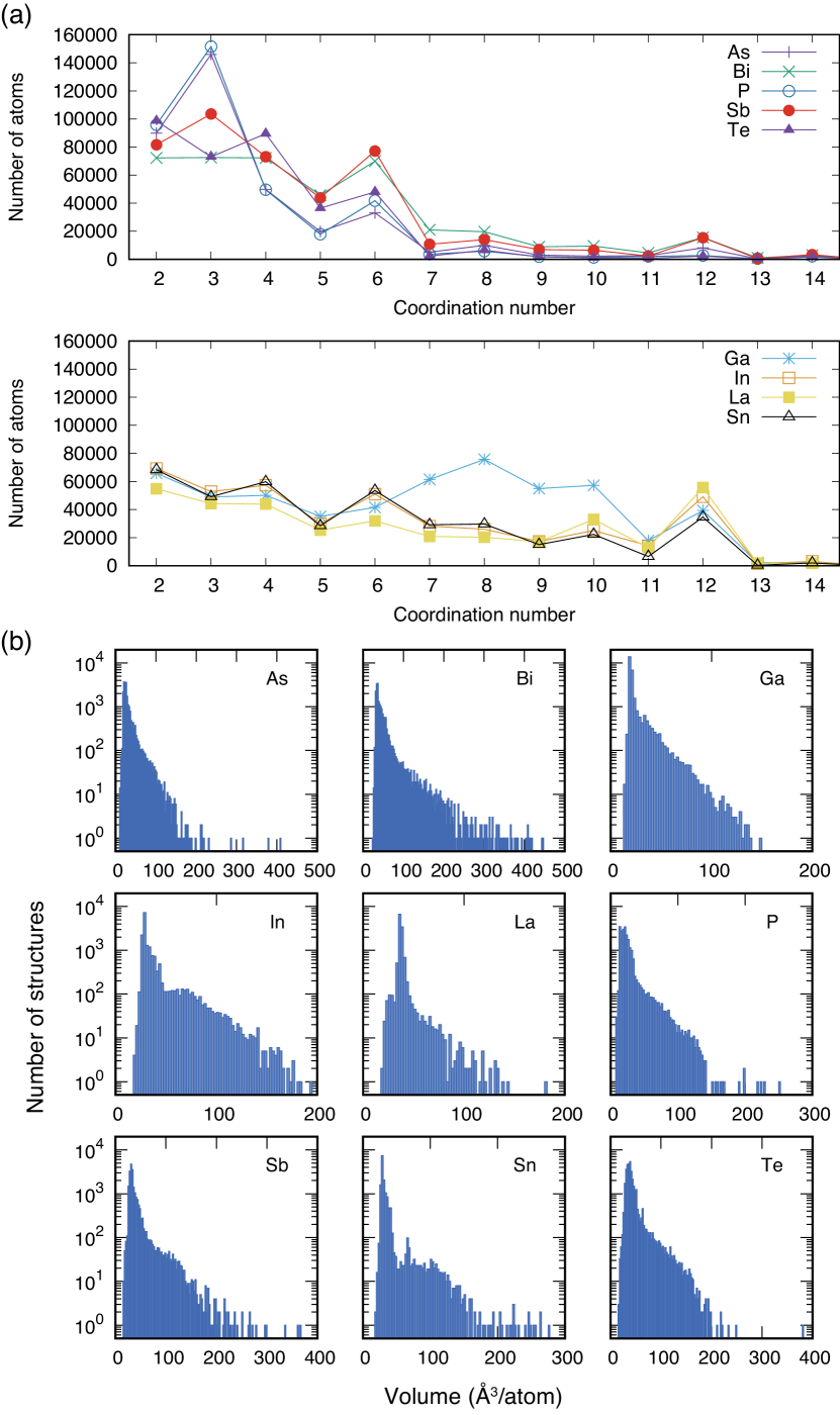
Figure 1: (a) Distribution of the coordination numbers around atoms in structures consisting of the training and test datasets. (b) Distribution of the volume for structures in the datasets. The distribution is displayed in the logarithmic scale for visibility.

Datasets for each elemental system were generated as follows. First, the atomic positions and lattice constants of 86 prototype structures Seko et al. (2019) using the DFT calculation were fully optimized. They comprise single elements with zero oxidation state from the Inorganic Crystal Structure Database (ICSD) Bergerhoff and Brown (1987), including metallic closed-packed structures, covalent structures, layered structures, and structures reported as high-pressure phases. Then, 13000–15000 structures were generated by randomly introducing lattice expansions, lattice distortions, and atomic displacements into supercells of optimized prototype structures. The entire set of structures was randomly divided into training and test datasets at a ratio of nine to one.

Figure 1 (a) displays the distribution of coordination numbers around atoms in structures that are present in both the training and test datasets. The datasets for the elements Ga, In, La, and Sn contain structures with coordination numbers ranging from two to twelve. However, the datasets for the elements As, Bi, P, Sn, and Te are biased and primarily composed of structures with coordination numbers ranging from two to eight. The coordination number distribution depends on the system, which arises from the variety of the converged prototype structures optimized by the DFT calculation. Although the DFT calculation optimizes the local geometry of the same prototype structure for each system, it converges to different structures based on the preferences of the neighborhood environment.

Figure 1 (b) shows the volume distribution of the datasets, displayed in a logarithmic scale for better visibility. The majority of the structures are distributed around the equilibrium volumes of the prototype structures. On the other hand, the maximum value of the volume in the distribution is nearly ten times the equilibrium volumes.

DFT calculations were performed for structures in the datasets using the plane-wave-basis projector augmented wave method Blöchl (1994) within the Perdew–Burke–Ernzerhof exchange-correlation functional Perdew et al. (1996) as implemented in the vasp code Kresse and Hafner (1993); Kresse and Furthmüller (1996); Kresse and Joubert (1999). The cutoff energy was set to 300 eV. The total energies converged to less than 10^-3 meV/supercell. The atomic positions and lattice constants of the prototype structures were optimized until the residual forces were less than 10^-2 eV/Å.

II.2.2 Regression

Weighted linear ridge regression was used to determine the regression coefficients for potential energy models. The energy values and force components in the training dataset were employed as observation entries in the regression. The forces acting on atoms are derived as linear models with the coefficients of the potential energy model, and the predictor matrix $\bm{X}$ and observation vector $\bm{y}$ can be written in a submatrix form as

$$\bm{X}=\begin{bmatrix}\bm{X}_{\rm energy}\\ \bm{X}_{\rm force}\\ \end{bmatrix},\qquad\bm{y}=\begin{bmatrix}\bm{e}\\ \bm{f}\\ \end{bmatrix}.$$ (10)

The matrix $\bm{X}_{\rm energy}$ comprises structural features and their polynomials, and the elements of $\bm{X}_{\rm force}$ are related to the derivatives of structural features with respect to the Cartesian coordinates of atoms, which were derived in Ref. Seko et al., 2019. The observation vector $\bm{y}$ includes components of $\bm{e}$ and $\bm{f}$, which contain the total energies and the forces acting on atoms in the training dataset, respectively. These values were obtained from DFT calculations.

Weighted linear ridge regression is a technique that can be used to shrink the regression coefficients by imposing a penalty. The approach involves minimizing the penalized residual sum of squares, which is given by

$$L(\bm{w})=||\bm{W}(\bm{X}\bm{w}-\bm{y})||_{2}^{2}+\lambda||\bm{w}||_{2}^{2},$$ (11)

where $\lambda$ and $\bm{W}$ denote the magnitude of the penalty and the diagonal matrix where non-zero elements correspond to weights for data entries, respectively. The solution to the minimization problem is represented by

$$\bm{\hat{w}}=(\bm{X}^{\top}\bm{W}^{2}\bm{X}+\lambda\bm{I})^{-1}\bm{X}^{\top}\bm{W}^{2}\bm{y},$$ (12)

where $\bm{I}$ denotes the unit matrix. The solution can be easily obtained using fast linear algebra algorithms while avoiding the well-known multicollinearity problem. In this study, the magnitude of the penalty is determined so that the estimated regression coefficients result in the lowest root mean square (RMS) error for an extensive test dataset.

The energy and forces acting on atoms have units that resemble weights for data entries. Specifically, the units eV/cell and eV/Å are used for defining energy and force, respectively. In addition, weights are applied to data entries depending on their values, which aims to develop robust MLPs for essential structures. This is achieved by decreasing the influence of less significant data entries that have large values. The weight for the energy entry of $i$-th structure $W(e_{[i]})$ is given as

$$W(e_{[i]})=\begin{cases}0.1&(e_{[i]}\geq 0)\\ 1&(e_{[i]}<0)\end{cases},$$ (13)

where $e_{[i]}$ denotes the total energy of structure $i$. Small weights are applied to energy entries of structures that are less stable than isolated atoms. The weight for the force entry on $\alpha$-component of atom $j$ in structure $i$, $W(f_{[i],j\alpha})$, is given as

$$W(f_{[i],j\alpha})=\begin{dcases}\frac{\varepsilon}{\left|f_{[i],j\alpha}\right|}&(|f_{[i],j\alpha}|\geq\varepsilon)\\ 1&(|f_{[i],j\alpha}|<\varepsilon)\end{dcases}.$$ (14)

Here, $\varepsilon$ is set to 1 eV/Å. Smaller weights are assigned to strong force components, whereas larger weights are given to weak force components observed in structures near local minima. This approach can help develop MLPs with high predictive power for structures near local minima.

II.2.3 Model selection

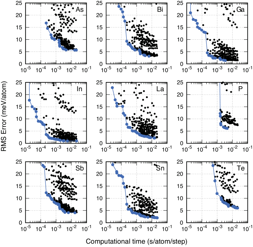
Figure 2: MLP distributions for nine different elements, including As, Bi, Ga, In, La, P, Sb, Sn, and Te, which are obtained through grid searches for finding optimal model parameters. The Pareto-optimal points of the distributions are shown by the blue closed circles. The computational efficiency is evaluated by measuring the elapsed time to compute the energy, forces, and stress tensors of a structure consisting of 284 atoms. The elapsed time is normalized by the number of atoms because it is proportional to the number of atoms. The elapsed time for a single point calculation is estimated using a single core of Intel® Xeon® E5-2695 v4 (2.10 GHz) and an implementation of the polynomial MLP to the lammps code Lam .

The accuracy and computational efficiency of polynomial MLPs depend on several input parameters. To find optimal MLPs with different trade-offs, a systematic grid search is performed. The input parameters in the grid search include the cutoff radius, the type of potential energy model, the number of radial functions, and the truncation of the polynomial invariants, i.e., the maximum angular numbers of spherical harmonics, $\{l_{\rm max}^{(2)},l_{\rm max}^{(3)},l_{\rm max}^{(4)},\cdots\}$, and the polynomial order of the invariants. Figure 2 shows the distributions of MLPs and the Pareto-optimal MLPs for the elemental As, Bi, Ga, In, La, P, Sb, Sn, and Te. The RMS error is used to estimate the prediction error for the energy values in the test dataset. As demonstrated in Fig. 2, the accuracy and computational efficiency of MLPs are conflicting properties, and the Pareto-optimal MLPs can be considered as suitable candidates for enumerating crystal structures.

For each system, an efficient MLP from the Pareto-optimal MLPs is chosen. This study focuses on crystal structure enumerations, so the selected MLP is desired to possess the following features: (1) The shape of the potential energy surface, particularly the locations of local minimum structures, should be reconstructed accurately. The MLP should be capable of predicting a wide variety of local minimum structures, ideally all of them. (2) The selected MLP should be able to recognize unrealistic and hypothetical structures with high DFT energy values as energetically unstable. MLP calculations must be performed for many such structures during crystal structure enumerations. (3) The potential energy surface of the MLP should have a limited number of ghost local minima. (4) The energy and force calculations done by the MLP should be computationally efficient since crystal structure enumerations involve performing many computations. Therefore, MLPs that require approximately 1 ms/atom for a single point calculation are selected.

Figure 3: Prediction errors of the selected MLPs for 86 prototype structures.

Figure 4: Distribution of the energy values for the training and test datasets, predicted using the DFT calculation and the selected MLPs.

Figure 3 shows the prediction errors of the selected MLPs for 86 prototype structures. As shown in Fig. 3, the MLPs have a high predictive power for various structures. Figure 4 displays the distributions of energies of structures in both the training and test datasets, computed using the DFT calculation and the polynomial MLP. The distributions demonstrate that the polynomial MLP is accurate for many typical structures and their derivatives containing diverse neighborhood environments and coordination numbers, as evidenced by a narrow distribution of errors. Overall, these results suggest that the polynomial MLPs are reliable for predicting the energies of a wide range of structures.

The MLPs shown here can be accessed through the Polynomial machine learning potential repository Seko (2023); Mac . While only their predictive power for energy has been demonstrated, the repository website includes predictions for other properties as well. Additionally, the predictive power for liquid states in the elemental Bi and Sn can be found elsewhere Wakai et al. (2024).

III Methodology on Structure enumeration

III.1 General statement

In a structure optimization problem with $N$ atoms at a given composition, a crystal structure can be represented by $3N+3$ independent variables $\bm{x}$. They do not contain the translational and rotational degrees of freedom. The goal of global structure optimization is to minimize the structure-dependent potential energy $E(\bm{x})$, formulated as

$$E^{*}=\min_{\bm{x}\in\mathbb{D}}E(\bm{x}),$$ (15)

within the nonempty feasible region $\mathbb{D}$ for crystal structure representation $\bm{x}$. The crystal structure that yields the minimum energy $E^{*}$ is denoted as the global minimum structure $\bm{x}^{*}$, hence $E^{*}=E(\bm{x}^{*})$. Similarly, a local minimum structure is denoted as $\bm{x}_{l}^{*}$, and a set of local minimum structures with energy values lower than a given energy threshold $\theta$ is denoted as

$$\mathbb{D}^{*}_{\theta}=\left\{\bm{x}_{l}^{*}\in\mathbb{D}\>|\>E(\bm{x}_{l}^{*})\leq\theta\right\}.$$ (16)

Depending on the choice of the crystal structure representation, multiple representations can correspond to the same structure, making the entire feasible region redundant. In addition, there may be subregions within the feasible region where it is impossible to form crystal structures. Furthermore, the feasible region contains physically unrealistic structures. To search for crystal structures efficiently, these unrealistic structures are often eliminated from the feasible region in advance. These subregions can be defined by constraints applied to the entire feasible region, particularly linear constraints. Given a set of constraints $\{g_{1}(\bm{x})\leq 0,\cdots,g_{m}(\bm{x})\leq 0\}$, the reduced feasible region $\Delta$ is described as

$$\Delta=\bigcap_{m}\Delta_{m},$$ (17)

where $\Delta_{m}$ denotes the feasible region reduced by constraint $g_{m}(\bm{x})\leq 0$, written as

$$\Delta_{m}=\{\bm{x}\in\mathbb{D}\>|\>g_{m}(\bm{x})\leq 0\}.$$ (18)

When the feasible region is reduced, the problems of finding the global minimum structure and enumerating local minimum structures are restated as

$$E^{*}=\min_{\bm{x}\in\Delta}E(\bm{x})$$ (19)

and

$$\Delta^{*}_{\theta}=\left\{\bm{x}_{l}^{*}\in\Delta\>|\>E(\bm{x}_{l}^{*})\leq\theta\right\},$$ (20)

respectively.

III.2 Computational procedures

This study employs a random structure search method [todo:cite]known as the multi-start approach for global optimization Hendrix et al. (2010). The approach involves repeatedly performing local geometry optimizations starting with uniformly sampled structures within the feasible region $\mathbb{D}$ or reduced feasible region $\Delta$. The random structure search is a reasonable approach for enumerating both global and local minimum structures. It is also simple to implement and can be parallelized easily.

The current procedure replaces most of the $ab$ $initio$ calculations in the $ab$ $initio$ random structure search (AIRSS) method Pickard and Needs (2011) with calculations using MLPs. However, there are some concerns about using MLPs for crystal structure enumerations. Firstly, MLPs often produce significant prediction errors for structures that are distant from the training dataset. It is impossible to prepare a training dataset that covers all local minimum structures in advance, so an iterative approach consisting of update processes of polynomial MLPs is used. Secondly, MLPs may produce small but non-negligible prediction errors, which make it difficult to assess the stability between local minimum structures using the energy values predicted by the MLPs. Therefore, the final stability between local minimum structures is evaluated using DFT calculations. The local geometry optimizations for the local minimum structures obtained using the MLP are systematically performed using DFT calculations.

The following is the current procedure for finding the global and local minimum structures: (1) A polynomial MLP is developed for the chosen model using DFT training and test datasets. (2) A large number of initial structures ($\sim 10^{5}$) are randomly and uniformly sampled from the reduced feasible region $\Delta$, which is limited to structures with up to twelve atoms. (3) Local geometry optimizations are systematically performed on the initial structures using the polynomial MLP. (4) Duplicate local minimum structures are identified and removed using space-group identification and a similarity measure that is closely related to the polynomial MLP (as described in Sec. III.3). A small tolerance value is used to eliminate duplicate structures, while ensuring that all borderline structures are kept as candidates for local minimum structures. (5) Single-point DFT calculations are performed for local minimum structures with low energy values, and their results are added to the training dataset. Steps (1)–(5) are repeated iteratively until a robust random structure search becomes possible. (6) Local geometry optimizations are then performed using the DFT calculation. These optimizations begin with a subset of local minimum structures with MLP energy values lower than a given threshold value $\theta^{\rm MLP}$. (7) Duplicate local minimum structures are again identified and removed using a tolerance value that is slightly larger than the one used in step (4).

The feasible region is defined by the metric tensor of lattice basis vectors and the fractional coordinates of the atomic positions with respect to the lattice basis vectors. This feasible region is then reduced by applying the main conditions for defining the Niggli reduced cell IUCr (2002). To create initial structures, a set of three diagonal components of the metric tensor is uniformly sampled, given an upper bound for the diagonal elements. Following the main conditions for the Niggli cell determined by the diagonal components, the non-diagonal components of the metric tensor are then randomly sampled between the upper and lower bounds. Although the fractional coordinates of the atomic positions in the reduced feasible region have duplicate subregions, the efficiency of the random structure search remains unaffected.

Note that the AIRSS can be computationally expensive because it requires numerous local geometry optimizations using $ab$ $initio$ calculations. To reduce the computational cost, initial structures are usually sampled within a feasible region based on prior knowledge of crystal structure stability. On the other hand, the current approach does not rely on any prior knowledge about the initial crystal structure, except for the upper bound of the metric tensor of lattice basis vectors, which is used to enumerate the global and local minimum structures in a robust manner.

III.3 Duplicate structure elimination

Numerous local geometry optimizations in steps (3) and (6) of the current procedure described in Sec. III.2 generate many duplicate structures. This issue has also been observed in global structure searches conducted elsewhere. To address this problem, the space group identification and a distance measure between structures defined by structural features to eliminate duplicate structures are used. These structure features are given in Eq. (2), which comprises the selected polynomial MLP. These structural features are then normalized with the regression coefficients of the selected polynomial MLP.

When indices of the structural features are written by single index $s=\{n,l_{1},l_{2},\cdots,l_{p},(\sigma)\}$, the averages of the normalized structural features and their products over atoms in structure $i$, $\bm{\bar{d}}_{[i]}$, are described as

$$\bm{\bar{d}}_{[i]}=\left[\cdots,\bar{d}_{[i],s},\cdots,\bar{d}_{[i],st},\cdots,\bar{d}_{[i],stu},\cdots\right],$$ (21)

where

$$\bar{d}_{[i],s} = \frac{1}{N_{[i]}}\sum_{k}w_{s}d_{[i],s}^{(k)},$$

$$\bar{d}_{[i],st} = \frac{1}{N_{[i]}}\sum_{k}w_{st}d_{[i],s}^{(k)}d_{[i],t}^{(k)},$$ (22)

$$\bar{d}_{[i],stu} = \frac{1}{N_{[i]}}\sum_{k}w_{stu}d_{[i],s}^{(k)}d_{[i],t}^{(k)}d_{[i],u}^{(k)},$$

and $N_{[i]}$ denotes the number of atoms in structure $i$. The distance between structures, $i$ and $j$, is then measured as the Euclidean distance of their corresponding $\bm{\bar{d}}_{[i]}$ and $\bm{\bar{d}}_{[j]}$, $\|\bm{\bar{d}}_{[i]}-\bm{\bar{d}}_{[j]}\|_{2}$. If the distance between the structures is small, they are considered similar in terms of the local neighboring atomic distribution. It is important to note that the current set of structural features is a generalization of radial distribution functions and angular distribution functions. These functions represent local neighboring atomic distributions and are often used to eliminate duplicate structures. (e.g., Valle and Oganov (2010)).

In the current structure searches using the MLPs, the number of local minimum structures frequently exceeds 50,000, which makes it impractical to compute distances for all pairs of structures. Therefore, an efficient procedure is introduced to eliminate duplicate structures. (1) Structures with different energy values are considered to be different. The energy value can act as a concise key to determine whether structures are different or not. This is based on the fact that the energy of structure $i$ is expressed using its normalized structural features as

$$E_{[i]}=\sum_{s}\bar{d}_{[i],s}+\sum_{st}\bar{d}_{[i],st}+\sum_{stu}\bar{d}_{[i],stu}+\cdots.$$ (23)

If the absolute difference between the energy values of structures $i$ and $j$ is more than a given tolerance parameter $\varepsilon_{E}$, $|E_{[i]}-E_{[j]}|>\varepsilon_{E}$, they are regarded as different. Here, the tolerance parameter is set to $\varepsilon_{E}=0.01$ meV/atom. If $|E_{[i]}-E_{[j]}|\leq\varepsilon_{E}$, we proceed to step (2). (2) Structures with different space groups are considered different. Because the space group identification depends on the tolerance parameter, multiple tolerance parameters are used. A single structure is identified with the set of space groups from the multiple tolerance parameters. If the sets of space groups for structures $i$ and $j$, $\{\mathbb{G}\}_{[i]}$ and $\{\mathbb{G}\}_{[j]}$, have no common elements, i.e., $\{\mathbb{G}\}_{[i]}\cap\{\mathbb{G}\}_{[j]}=\varnothing$, the structures are regarded to be different. Otherwise, we proceed to step (3). (3) Two structures separated by a distance larger than a tolerance parameter $\varepsilon_{d}$, i.e., $\|\bm{\bar{d}}_{[i]}-\bm{\bar{d}}_{[j]}\|_{2}>\varepsilon_{d}$, are considered different. Here, the tolerance parameter is set to $\varepsilon_{d}=0.001$. Otherwise, they are regarded to be identical.

Note that the distances between structures that are clearly identical are less than $10^{-7}$. Alternatively, the distances between structures that are visibly different but have similar energy values are greater than 0.1. Most structure pairs are classified into either the first or second category, while some pairs lie on the borderline. In the case of a set of local minimum structures obtained using the DFT calculation, the tolerance parameters of $\varepsilon_{E}=1$ meV/atom and $\varepsilon_{d}=0.01$ are employed. These values are larger than those used for structures obtained using MLPs, due to the adoption of larger convergence criteria for local geometry optimizations using the DFT calculation.

IV Crystal structure enumeration

Structure enumerations begin with polynomial MLPs that are developed using the procedure outlined in Section II.2. These MLPs are created from datasets generated from various prototype structures, and they are generally accurate for many local minimum structures. However, the MLPs sometimes produce ghost local minimum structures and fail to predict the energy for some local minimum structures with accuracy. Therefore, the MLPs are iteratively improved using the DFT datasets for structures that are predicted to be local minima by the MLPs. These DFT datasets are then added to the training datasets, as demonstrated in Section III.2.

Table 1: Accuracy and computational efficiency of the polynomial MLPs that are iteratively updated using DFT data for the global and local minimum structures. These structures are obtained from random structure searches using the MLPs. The RMS errors are calculated for a test dataset to evaluate the performance of the updated MLPs.

	RMS error (energy)	RMS error (force)	Time
	(meV/atom)	(eV/Å)	(ms/atom/step)
As	9.4	0.137	3.0
Bi	3.8	0.060	1.8
Ga	2.1	0.032	1.6
In	1.0	0.015	1.0
La	3.2	0.057	2.1
P	8.5	0.169	2.6
Sb	4.2	0.070	3.0
Sn	2.6	0.042	1.9
Te	8.4	0.102	5.5

Table 1 lists the RMS errors of the updated MLPs at the final iteration. The RMS errors are estimated using the same test datasets that were employed in developing the MLPs without incorporating the DFT dataset obtained from structure enumerations. To provide practically useful measures of accuracy, the RMS errors are calculated by removing structures that exhibit extremely high energies and strong forces. For the elemental Bi, Ga, In, La, Sb, and Sn, the updated MLPs not only maintain their predictive power for the original datasets but also enhance the predictive power for the global and local minimum structures. However, for the elemental As, P, and Te, although the updated MLPs significantly improve the predictive power for the global and local minimum structures, the updates of the MLPs slightly decrease the predictive power for the original datasets.

Random structure searches are then carried out using the updated MLPs, repeating numerous local geometry optimizations systematically. From these searches, unique local minimum structures with MLP energy values, $E^{\rm MLP}$, lower than a given energy threshold $\theta^{\rm MLP}$, $E^{\rm MLP}\leq\theta^{\rm MLP}$, are extracted. To ensure reliable structure enumerations, the following threshold values are used: 25 meV/atom for Ga, 50 meV/atom for As, Bi, and In, 75 meV/atom for La, P, Sb, and Sn, and 100 meV/atom for Te, which are measured from the lowest energy. Although different threshold values are also possible, these threshold values are chosen because the current results of structure enumerations are reliable for them.

When it is assumed that the Bayesian estimates on the number of local minima in multi-start approaches Boender and Rinnooy Kan (1987) are applicable to the current structure search, the estimates are calculated for $E^{\rm MLP}\leq\theta^{\rm MLP}$ as follows: 465.9, 189.8, 1566.7, 520.1, 298.9, 282.7, 407.6, 403.3, 418.9 for As, Bi, Ga, In, La, P, Sb, Sn, and Te, respectively. These estimates are very close to the numbers of the local minimum structures found in the current random structure searches, i.e., 464, 189, 1529, 516, 297, 282, 406, 400, and 417, respectively. This indicates that most of the local minimum structures with $E^{\rm MLP}\leq\theta^{\rm MLP}$ existing in the feasible region should be found in the current structure searches using the MLPs, including the globally stable structure.

Figure 5: Energy distribution for the global and local minimum structures. The MLP energy is calculated using the updated MLP at the final iteration.

Once a set of local minimum structures with $E^{\rm MLP}\leq\theta^{\rm MLP}$ is obtained using the MLP, local geometry optimizations are performed using the DFT calculation. This allows us to evaluate the stability of the structures more accurately. Figure 5 shows the energy distribution of the local minimum structures in the nine elemental systems. The energy values of the local minimum structures predicted using the DFT calculation and the polynomial MLP show strong correlations as a result of the iterative update of the MLPs. This result suggests that the updated MLPs can accurately enumerate most of the local minimum structures with low energy values. However, there are some local minimum structures whose energies predicted by the polynomial MLPs deviate from their DFT energies. While the MLPs are less reliable in predicting the energy of such structures, they can still play an adequate role in finding local minimum structures with low energy values. If we aim to improve the predictive power for such structures, more complex models for the MLPs are necessary.

Table 2: Number of the global and local minimum structures for several energy threshold values $\theta$. The energy values of the local minimum structures are computed using the DFT calculation. The energy threshold values are described in the unit of meV/atom.

	$\theta=5$	$\theta=10$	$\theta=15$	$\theta=20$	$\theta=25$
Ga	1	101	616	902	1142
	$\theta=10$	$\theta=20$	$\theta=30$	$\theta=40$	$\theta=50$
As	269	336	387	407	415
Bi	2	11	27	54	101
In	99	113	135	336	474
	$\theta=15$	$\theta=30$	$\theta=45$	$\theta=60$	$\theta=75$
La	73	150	205	220	253
P	112	191	255	274	276
Sb	2	24	101	220	302
Sn	1	4	13	81	310
	$\theta=20$	$\theta=40$	$\theta=60$	$\theta=80$	$\theta=100$
Te	7	41	81	253	339

Table 2 shows the number of unique local minimum structures obtained using the DFT calculation. The table shows the number of structures with DFT energy values lower than $\theta^{\rm MLP}$ and those with DFT energy values lower than threshold values $\theta$, which are lower than $\theta^{\rm MLP}$, $E^{\rm DFT}\leq\theta<\theta^{\rm MLP}$. It can be observed that there are many local minimum structures with energy values that are very close to the global minimum energy in these systems.

However, the use of the DFT calculation causes a reduction in the number of unique local minimum structures. Some structures have MLP energy values lower than $\theta^{\rm MLP}$, but their DFT energy values are larger than $\theta^{\rm MLP}$, $E^{\rm DFT}>\theta^{\rm MLP}$. Similarly, some structures with MLP energy values higher than $\theta^{\rm MLP}$ can exhibit DFT energy values smaller than $\theta^{\rm MLP}$, $E^{\rm DFT}\leq\theta^{\rm MLP}$. Therefore, the set of global and local minimum structures for a threshold lower than $\theta^{\rm MLP}$ is more reliable. On the other hand, the set of structures for $\theta\sim\theta^{\rm MLP}$ is expected to become larger than shown in Table 2.

The decrease in the number of structures also originates from the current setting of tolerance parameters to eliminate duplicate structures. Specifically, a larger tolerance value is used for the structures obtained through the DFT calculation in comparison to those obtained using the MLPs, which is explained in Sec. III.2. Moreover, some of the converged structures are duplicated, but the majority of the structures obtained through the MLPs converge to unique local minimum structures in DFT geometry optimizations.

IV.1 As

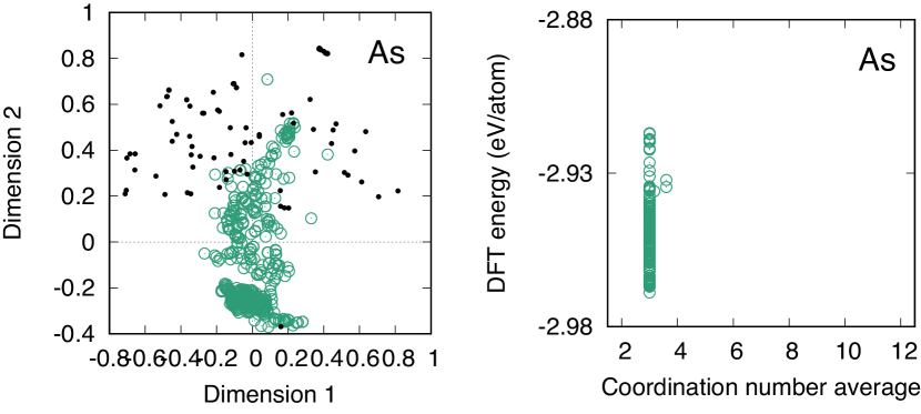
Figure 6: (a) Distribution of the local minimum structures and equilibrium prototype structures in As. The prototype structures are used to derive structures in the training dataset. These structures are mapped into a two-dimensional plane using an MDS for visibility. The open and closed circles show the local minimum structures and prototype structures, respectively. (b) Average coordination numbers of the local minimum structures. The cutoff radius is given as 1.2 times the nearest neighbor distance.

In the elemental As, it is found that there are 415 local minimum structures that have relative energy values lower than $\theta=50$ meV/atom. Specifically, 269 of those structures have relative energy values less than $\theta=10$ meV/atom. Figure 6 (a) displays the distribution of local minimum structures and equilibrium prototype structures that are used to create structures in the training dataset. The structural features of the polynomial MLP for these structures are mapped onto a two-dimensional plane using multi-dimensional scaling (MDS) Borg and Groenen (2005). Figure 6 (a) also provides a visual representation of the similarity measure between the local minimum structures and training dataset. As shown in the figure, many local minimum structures are located far from the prototype structures. Figure 6 (b) shows the distribution of average coordination numbers for the local minimum structures. The cutoff radius used is 1.2 times the nearest neighbor distance. The global minimum structure and most of the local minimum structures are three-coordinated, which is consistent with the experimental structure.

Table 3: Global and local minimum structures in As. The relative energy $\Delta E$ calculated using the DFT calculation is expressed in the unit of meV/atom. $Z$ denotes the number of atoms included in the unitcell. Parentheses in the columns of ICSD identifiers and prototype structures indicate that the corresponding structure is close to the prototype in the parentheses. However, its space group is different from that of the prototype structure and/or large tolerance values are required for the prototype identification.

Space group	ICSD-ID	Prototype	$Z$	$\Delta E$
$R\bar{3}m$	9859	As	6	0.0
$P\bar{3}m1$	(1425)	(HCP)	2	1.9
$C2/m$	(1425)	(HCP)	8	2.0
$P\bar{3}m1$	(1425)	(HCP)	4	2.0
$R\bar{3}m$	$-$	$-$	24	2.1
$R\bar{3}m$	$-$	$-$	30	2.1
$P3m1$	$-$	$-$	6	2.1
$P3m1$	(31170)	(C($P6_{3}mc$))	4	2.1
$R\bar{3}m$	$-$	$-$	18	2.2
$R\bar{3}m$	$-$	$-$	12	2.2
$P6_{3}mc$	31170	C($P6_{3}mc$)	4	2.2
$P\bar{3}m1$	$-$	$-$	8	2.2
$R3m$	$-$	$-$	12	2.2
$R\bar{3}m$	$-$	$-$	18	2.2
$R\bar{3}m$	$-$	$-$	18	2.2
$R\bar{3}m$	$-$	$-$	12	2.3
$R\bar{3}m$	$-$	$-$	18	2.3
$R3m$	$-$	$-$	24	2.3
$R3m$	$-$	$-$	24	2.4
$R3m$	$-$	$-$	30	2.4
$R3m$	$-$	$-$	24	2.4
$R3m$	$-$	$-$	24	2.5
$R3m$	$-$	$-$	24	2.5
$R3m$	$-$	$-$	30	2.5
$R3m$	$-$	$-$	36	2.5
$P3m1$	$-$	$-$	10	2.5
$P1$	$-$	$-$	10	2.5
$R3m$	$-$	$-$	30	2.5
$R3m$	$-$	$-$	18	2.5
$C2/m$	2284	O2($mS4$)	4	3.2
$R\bar{3}m$	29213	Graphite(3R)	6	3.2
$R\bar{3}m$	29213	Graphite(3R)	6	3.8
$P6_{3}mc$	31170	C($P6_{3}mc$)	4	4.1
$Cmce$	23836	black-P	8	18.7

Table 3 provides a list of local minimum structures found in the elemental As. This list includes only the structures that have low energy values and can be identified with prototype structures and experimental structures in As. Prototype identifiers that are consistent with the ICSD are given. The global minimum structure is the three-coordinated As-type structure, which is consistent with the experimental structure at low temperatures Schiferl and Barrett (1969); Young (1991). Apart from the global minimum structure, three-coordinated structures such as C($P6_{3}mc$)-, graphite(3R)-, and black-P-type are also found as local minimum structures. However, among these structures, only the black-P-type structure is an experimental polymorph Smith et al. (1975).

IV.2 Bi

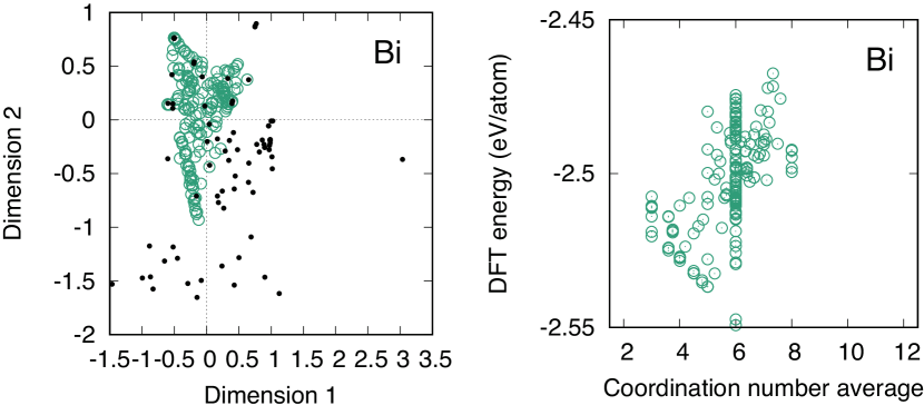
Figure 7: (a) Distribution of the local minimum structures and equilibrium prototype structures in Bi. These structures are mapped into a two-dimensional plane using an MDS. The open and closed circles show the local minimum structures and prototype structures, respectively. (b) Average coordination numbers of the local minimum structures. The cutoff radius is given as 1.2 times the nearest neighbor distance.

In the elemental Bi, 101 different local minimum structures with relative energy values lower than $\theta=$ 50 meV/atom have been discovered. The distribution of these local minimum structures and equilibrium prototype structures in Bi is shown in Fig. 7 (a). The majority of the local minimum structures are located around the equilibrium prototype structures. Figure 7 (b) shows the distribution of average coordination numbers for the local minimum structures in Bi. The global minimum structure is six-coordinated, and the average coordination numbers of the local minimum structures in Bi range from three to eight.

Table 4: Global and local minimum structures in Bi. The DFT relative energy $\Delta E$ is expressed in the unit of meV/atom. $Z$ denotes the number of atoms included in the unitcell.

Space group	ICSD-ID	Prototype	$Z$	$\Delta E$
$R\bar{3}m$	9859	As	6	0.0
$Imma$	(9859)	(As)	4	1.8
$R\bar{3}m$	$-$	$-$	36	12.5
$P\bar{3}m1$	$-$	$-$	12	12.5
$P3m1$	$-$	$-$	10	13.8
$P\bar{3}m1$	$-$	$-$	10	14.6
$R3m$	$-$	$-$	24	16.7
$P\bar{3}m1$	$-$	$-$	8	16.7
$P6_{3}mc$	$-$	$-$	8	16.8
$R\bar{3}m$	$-$	$-$	24	17.6
$C2/m$	$-$	$-$	24	19.8
$Cm$	$-$	$-$	24	20.4
$R3m$	$-$	$-$	18	20.9
$R\bar{3}m$	$-$	$-$	18	21.4
$R3m$	$-$	$-$	36	21.8
$R\bar{3}m$	$-$	$-$	18	22.0
$P\bar{3}m1$	$-$	$-$	6	22.2
$P2_{1}/m$	$-$	$-$	10	23.5
$R3m$	$-$	$-$	30	24.2
$R3m$	$-$	$-$	30	25.0
$P3m1$	$-$	$-$	10	25.0
$P6_{3}mc$	31180	C($P6_{3}mc$)	4	28.9
$P2_{1}/m$	(43211)	(SC)	8	38.7
$C2$	(43211)	(SC)	18	39.6
$P1$	(43211)	(SC)	12	39.7
$Pm\bar{3}m$	43211	SC	1	40.0
$I4_{1}/amd$	40037	$\beta$-Sn	4	41.1
$Pnma$	165995	MnP	8	41.6
$C2/m$	409752	Bi(II)	20	42.9
$Cmce$	23836	black-P	8	49.4
$I4_{1}/amd$	109018	Cs(HP)	4	49.8

Table 4 lists the local minimum structures found in the elemental Bi. The global minimum structure is the As-type structure, which is consistent with the experimental structure observed at low temperatures Davey (1925); Cucka and Barrett (1962); Young (1991). It is worth noting that the global minimum structure can be considered as six-coordinated, which is different from the three-coordinate As-type structure observed in the elemental As. This inconsistency is due to the fact that the distribution of interatomic distances in the As-type structure for Bi is different from that in the As-type structure for As.

Moreover, some of the local minimum structures are assigned as prototype structures, such as C($P6_{3}mc$)-, simple-cubic (SC)-, $\beta$-Sn-, MnP-, Bi(II)-, black-P-, and Cs(HP)-type structures. Among these structures, the SC-type Jaggi (1964) and Bi(II)-type Akselrud et al. (2003) structures were reported as high-pressure polymorphs in the literature. The body-centered-cubic (BCC)-type structure, which is known as a high-pressure structure Schaufelberger et al. (1973), is also found in the structure list obtained from the structure search using the MLPs. However, it exhibits a relative energy value larger than $\theta=$ 50 meV/atom. In the elemental Bi, Bi($I4/mcm$)-type Degtyareva et al. (2001), Bi(III)-type Degtyareva et al. (2001), Si($oS16$)-type Chaimayo et al. (2012), and Sb($mP4$)-type Kabalkina et al. (1970) structures were also reported as high-pressure phases, but they are not found in the current structure list.

IV.3 Ga

Figure 8: (a) Distribution of the local minimum structures and equilibrium prototype structures in Ga. These structures are mapped into a two-dimensional plane using an MDS. The open and closed circles show the local minimum structures and prototype structures, respectively. (b) Average coordination numbers of the local minimum structures. The cutoff radius is given as 1.2 times the nearest neighbor distance.

There are 1142 local minimum structures in the elemental Ga with relative energy values less than $\theta=$ 25 meV/atom. Among these structures, 616 structures are highly competitive in terms of energy, with relative energy values less than 15 meV/atom. Figure 8 (a) shows the distribution of the local minimum structures and equilibrium prototype structures in Ga. The local minimum structures are located inside the distribution of the prototype structures, while many of them are distant from the prototype structures. Figure 8 (b) shows the distribution of average coordination numbers for the local minimum structures in Ga. The global minimum structure has a coordination number of seven, while 12-coordinated local minimum structures similar to the FCC structure are also competing with the global minimum structure. The average coordination numbers of the local minimum structures in Ga range from six to twelve.

Table 5: Global and local minimum structures in Ga. The DFT relative energy $\Delta E$ is expressed in the unit of meV/atom. $Z$ denotes the number of atoms included in the unitcell.

Space group	ICSD-ID	Prototype	$Z$	$\Delta E$
$Cmce$	43388	Ga(I)	8	0.0
$P\bar{1}$	(12174)	(In)	10	5.2
$C2/m$	(12174)	(In)	16	5.4
$Cmcm$	$-$	$-$	8	5.5
$P\bar{1}$	(12174)	(In)	12	5.5
$Imma$	$-$	$-$	16	5.6
$P\bar{1}$	(12174)	(In)	12	5.8
$P1$	(12174)	(In)	12	5.8
$C2/m$	(54338)	(Pr)	24	5.9
$C2/m$	(54338)	(Pr)	18	6.1
$P\bar{1}$	(12174)	(In)	12	6.1
$Cmcm$	$-$	$-$	24	6.9
$R\bar{3}m$	(12174)	(In)	3	7.3
$Cmmm$	$-$	$-$	22	7.6
$Cmcm$	$-$	$-$	4	7.6
$Cm$	$-$	$-$	24	7.8
$Immm$	$-$	$-$	22	7.8
$Fm\bar{3}m$	20502	FCC	4	7.9
$Cm$	$-$	$-$	16	8.0
$Cm$	$-$	$-$	20	8.1
$R\bar{3}m$	$-$	$-$	30	8.1
$Fddd$	44866	Pu($oF8$)	8	8.1
$C2/c$	$-$	$-$	20	8.2
$Immm$	$-$	$-$	22	8.2
$Cmmm$	$-$	$-$	18	8.2
$P4_{2}2_{1}2$	$-$	$-$	8	8.3
$R\bar{3}m$	$-$	$-$	27	8.3
$Cm$	(52496)	(Tb)	12	8.3
$Cmce$	$-$	$-$	16	8.4
$Cmcm$	$-$	$-$	16	8.4
$Cm$	$-$	$-$	16	8.4
$Cm$	(43573)	(La)	16	8.7
$P6_{3}/mmc$	43573	La	4	9.5
$Cmcm$	43539	Ga($Cmcm$)	4	9.6
$P6_{3}/mmc$	52496	Tb	6	9.8
$C2/m$	2284	O2($mS4$)	20	10.1
$Pnma$	165995	MnP	8	10.8
$P6_{3}/mmc$	164724	O2	4	11.2
$R3c$	(12173)	(Ga(II))	18	11.7
$P2_{1}/c$	189806	Bi($P2_{1}/c$)	8	12.3
$R\bar{3}m$	52497	Sm	9	12.9
$I\bar{4}3d$	109012	Li($cI16$)	16	15.0
$P6_{3}/mmc$	1425	HCP	2	16.1
$P3_{2}21$	281124	S	9	22.0
$P2_{1}2_{1}2$	16817	H2O(III,IX)	12	23.8

Table 5 presents a list of the local minimum structures in the elemental Ga. The global minimum structure is the Ga(I)-type structure with the space group of $Cmce$, which is the experimental structure observed at low temperatures Sharma and Donohue (1962); Young (1991). One of the local minimum structures, exhibiting the fourth lowest energy value and the space group of $Cmcm$, corresponds to a metastable structure determined through first-principle prediction de Koning et al. (2009).

In the elemental Ga, there are numerous competing close-packed and open structures. The close-packed structures include In-, face-centered-cubic (FCC)-, La-, and Sm-type structures, while the open structures with coordination numbers of seven and eight correspond to Ga(I)- and Ga($Cmcm$)-type structures. Intermediate structures between the open and close-packed structures, namely Pu($oF8$)-, Ga(II)-, and Li($cI16$)-types, are also found as local minimum structures.

Experimental studies reported Ga($Cmcm$)- Defrain et al. (1961), In- (Ga(III)-) Bosio (2008), Ga(II)- Bosio (2008), and Ga($R\bar{3}m$)($\delta$Ga)-type Bosio et al. structures. The first three structures are present in the list of local minimum structures. Although the Ga(II)-type structure is not equivalent to but close to a local minimum structure with a different space group, $R3c$. The Ga($R\bar{3}m$)($\delta$Ga)-type structure requires at least 22 atoms to represent, which cannot be discovered in the current procedure.

IV.4 In

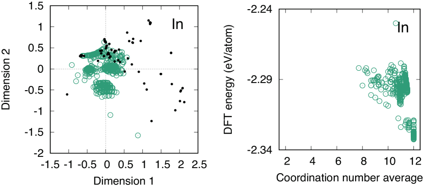
Figure 9: (a) Distribution of the local minimum structures and equilibrium prototype structures in In. These structures are mapped into a two-dimensional plane using an MDS. The open and closed circles show the local minimum structures and prototype structures, respectively. (b) Average coordination numbers of the local minimum structures. The cutoff radius is given as 1.2 times the nearest neighbor distance.

A total of 474 local minimum structures with relative energy values less than $\theta=$ 50 meV/atom have been discovered in the elemental In. Among them, 99 structures are found for $\theta=5$ meV/atom. Figure 9 (a) shows the distribution of the local minimum structures and equilibrium prototype structures in the elemental In. Some local minimum structures are close to the equilibrium prototype structures, while many others are far from them. Figure 9 (b) shows the distribution of average coordination numbers for the local minimum structures in the elemental In. The global minimum structure is 12-coordinated, and the local minimum structures also exhibit large coordination numbers ranging from 10 to 12.

Table 6: Global and local minimum structures in In. The DFT relative energy $\Delta E$ is expressed in the unit of meV/atom. $Z$ denotes the number of atoms included in the unitcell.

Space group	ICSD-ID	Prototype	$Z$	$\Delta E$
$C2/m$	(12174)	(In)	20	0.0
	(57392)	(In($Fmmm$))
	(41824)	(Ce)
$I4/mmm$	12174	In	2	0.1
$C2/m$	54338	Pr	4	0.4
$C2/m$	(12174)	(In)	16	0.4
$C2/m$	41824	Ce	2	0.6
$P\bar{1}$	(41824)	(Ce)	1	1.0
$Pmmn$	(12174)	(In)	10	1.2
$C2/m$	$-$	$-$	24	1.6
$C2/m$	$-$	$-$	18	1.7
$R\bar{3}m$	$-$	$-$	24	1.8
$C2/m$	$-$	$-$	24	1.8
$P6_{3}/mmc$	$-$	$-$	8	1.8
$Cmcm$	$-$	$-$	20	1.9
$R\bar{3}m$	$-$	$-$	27	1.9
$P\bar{6}m2$	$-$	$-$	12	1.9
$C2/m$	$-$	$-$	20	1.9
$R\bar{3}m$	$-$	$-$	24	2.0
$C2/m$	$-$	$-$	20	2.0
$P\bar{3}m1$	$-$	$-$	9	2.1
$C2/m$	$-$	$-$	22	2.1
$C2/m$	$-$	$-$	20	2.2
$R\bar{3}m$	$-$	$-$	18	2.2
$P6_{3}/mmc$	43573	La	4	2.3
$C2/m$	$-$	$-$	18	2.3
$C2/m$	$-$	$-$	16	2.3
$R\bar{3}m$	$-$	$-$	30	2.3
$P\bar{3}m1$	$-$	$-$	7	2.4
$R3m$	$-$	$-$	36	2.4
$R3m$	$-$	$-$	33	2.4
$P6_{3}/mmc$	52496	Tb	6	2.6
$R\bar{3}m$	52497	Sm	9	5.3
$P6_{3}/mmc$	1425	HCP	2	5.7
$I\bar{4}3d$	109012	Li($cI16$)	16	8.7
$P1$	(5248)	(BCC)	11	10.3
$P3_{2}21$	281124	S	9	38.3

Table 6 provides a list of the local minimum structures present in the elemental In. The global minimum structure has the $C2/m$ space group, is 12-coordinated, and is almost identical to the In-type Hull and Davey (1921) and In($Fmmm$)-type Takemura and Fujihisa (1993) structures. However, the high-pressure In($Fmmm$)-type structure, reported in the literature, is quite different from the global minimum structure in terms of the lattice constants. The local minimum structure with the second lowest energy can be identified with the In-type structure, which is the experimental structure at room temperature Hull and Davey (1921); Young (1991). Table 6 shows that there are many local minimum structures with low relative energy values, including La-, Tb-, Sm-, and hexagonal-close-packed (HCP)-type structures. In the literature, the In- and In($Fmmm$)-type structures are included in the ICSD. They are found in the list of local minimum structures.

IV.5 La

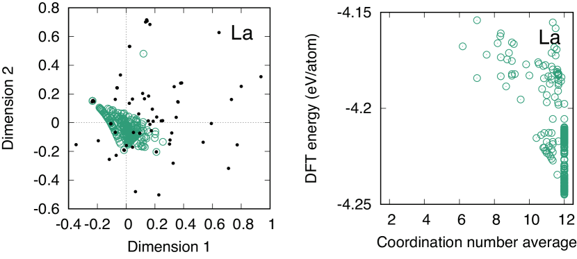
Figure 10: (a) Distribution of the local minimum structures and equilibrium prototype structures in La. These structures are mapped into a two-dimensional plane using an MDS. The open and closed circles show the local minimum structures and prototype structures, respectively. (b) Average coordination numbers of the local minimum structures. The cutoff radius is given as 1.2 times the nearest neighbor distance.

In the case of the elemental La, 253 local minimum structures have been identified, all of which have relative energy values less than $\theta=$ 75 meV/atom. Among these structures, 73 structures have been discovered for $\theta=15$ meV/atom. Figure 10 (a) shows the distribution of the local minimum structures and equilibrium prototype structures in La. Many local minimum structures are distributed around the equilibrium prototype structures. Figure 10 (b) depicts the distribution of average coordination numbers for the local minimum structures in La. The global minimum structure and many local minimum structures are 12-coordinated, while some local minimum structures have smaller coordination numbers ranging from six to eight.

Table 7: Global and local minimum structures in La. The DFT relative energy $\Delta E$ is expressed in the unit of meV/atom. $Z$ denotes the number of atoms included in the unitcell.

Space group	ICSD-ID	Prototype	$Z$	$\Delta E$
$P6_{3}/mmc$	43573	La	4	0.0
$R\bar{3}m$	$-$	$-$	27	0.3
$R\bar{3}m$	$-$	$-$	15	0.7
$P\bar{6}m2$	$-$	$-$	10	1.2
$R3m$	$-$	$-$	33	1.3
$R\bar{3}m$	$-$	$-$	33	1.4
$R\bar{3}m$	$-$	$-$	18	1.6
$P\bar{3}m1$	$-$	$-$	7	1.7
$R\bar{3}m$	$-$	$-$	24	1.9
$R\bar{3}m$	$-$	$-$	33	1.9
$R3m$	$-$	$-$	36	2.1
$R\bar{3}m$	$-$	$-$	21	2.3
$R\bar{3}m$	$-$	$-$	27	2.3
$P\bar{3}m1$	$-$	$-$	9	2.4
$R\bar{3}m$	$-$	$-$	21	2.8
$P6_{3}/mmc$	$-$	$-$	8	2.8
$P6_{3}/mmc$	52496	Tb	6	2.9
$P6_{3}/mmc$	$-$	$-$	10	2.9
$P\bar{3}m1$	$-$	$-$	8	3.0
$P3m1$	$-$	$-$	9	3.4
$R3m$	$-$	$-$	33	3.4
$R3m$	$-$	$-$	30	3.7
$P3m1$	$-$	$-$	12	3.8
$R3m$	$-$	$-$	24	4.1
$R3m$	$-$	$-$	36	4.1
$P3m1$	$-$	$-$	10	4.4
$P3m1$	$-$	$-$	11	4.4
$R3m$	$-$	$-$	33	4.6
$Fm\bar{3}m$	20502	FCC	4	4.7
$R3m$	$-$	$-$	27	4.8
$P\bar{3}m1$	$-$	$-$	9	5.0
$R\bar{3}m$	52497	Sm	9	6.2
$P6_{3}/mmc$	1425	HCP	2	29.5
$P6/mmm$	52521	CaHg2	3	29.7

The local minimum structures in the elemental La are listed in Table 7. The 12-coordinated La-type structure is the global minimum structure, which is consistent with the experimental structure at low temperatures Spedding et al. (1961); Young (1991). Additionally, several close-packed local minimum structures, such as the FCC-, Sm-, and HCP-type structures, have low energy values near the global minimum energy. Among these structures, the FCC-type structure is recognized as a high-temperature polymorph Spedding et al. (1961); Young (1991). Although the BCC-type structure is also known as a high-temperature structure Spedding et al. (1961); Young (1991), it is not found in the structure list since it is dynamically unstable at zero temperature. Moreover, the Sn($tI2$)-type structure Nomura et al. (1977) is not included in the structure list.

IV.6 P

Figure 11: (a) Distribution of the local minimum structures and equilibrium prototype structures in P. These structures are mapped into a two-dimensional plane using an MDS. The open and closed circles show the local minimum structures and prototype structures, respectively. (b) Average coordination numbers of the local minimum structures. The cutoff radius is given as 1.2 times the nearest neighbor distance.

In this study, 276 local minimum structures with relative energy values less than $\theta=$ 75 meV/atom have been identified for the elemental P. In particular, 112 structures are discovered for $\theta=15$ meV/atom. Figure 11 (a) shows the distribution of the local minimum structures and equilibrium prototype structures in P. Most of the local minimum structures are located far from the equilibrium prototype structures. Figure 11 (b) presents the distribution of average coordination numbers for the local minimum structures in P. The global minimum structure and most of the local minimum structures have three-coordinated configurations.

Table 8: Global and local minimum structures in P. The DFT relative energy $\Delta E$ is expressed in the unit of meV/atom. $Z$ denotes the number of atoms included in the unitcell.

Space group	ICSD-ID	Prototype	$Z$	$\Delta E$
$Cmce$	23836	black-P	8	0.0
$Ibam$	$-$	$-$	16	3.0
$C2/m$	$-$	$-$	20	3.1
$P\bar{1}$	$-$	$-$	12	3.1
$C2/m$	$-$	$-$	12	4.1
$P\bar{1}$	$-$	$-$	12	4.1
$P\bar{1}$	$-$	$-$	8	4.5
$Cm$	$-$	$-$	24	4.6
$C2/m$	$-$	$-$	24	4.7
$C2/m$	$-$	$-$	24	4.8
$P\bar{1}$	$-$	$-$	6	5.3
$C2/m$	$-$	$-$	20	5.5
$Cccm$	$-$	$-$	8	5.9
$P2/m$	$-$	$-$	12	6.1
$C2/m$	$-$	$-$	16	6.3
$C2/m$	$-$	$-$	16	6.3
$P2/m$	$-$	$-$	12	6.3
$P\bar{1}$	$-$	$-$	12	7.2
$Cm$	$-$	$-$	24	7.2
$Pm$	$-$	$-$	12	7.3
$C2/m$	$-$	$-$	20	7.4
$C2/m$	$-$	$-$	20	7.7
$P\bar{1}$	$-$	$-$	8	7.7
$C2/m$	$-$	$-$	24	8.0
$P\bar{3}m1$	(1425)	(HCP)	2	10.4
$P6_{3}mc$	31170	C($P6_{3}mc$)	4	10.5
$R\bar{3}m$	29123	Graphite(3R)	6	10.7
$I2_{1}3$	187643	N	8	35.2
$R\bar{3}m$	9859	As	6	50.3

Table 8 lists the local minimum structures in the elemental P. The global minimum structure is the three-coordinated black-P-type structure, also known as the most stable experimental structure at room temperature Brown and Rundqvist (1965); Young (1991). The structure list includes many other three-coordinated local minimum structures such as the C($P6_{3}mc$)-, graphite(3R)-, and As-type structures. However, only the As-type structure is known as a high-pressure polymorph Jamieson (1963); Young (1991). Several other experimental structures such as the SC- Kikegawa and Iwasaki (1983); Young (1991), Ca(III)- Marqués et al. (2008), P($Amm2$)-types Marqués et al. (2008) have also been reported as high-pressure polymorphs in the literature. Among these structures, only the SC-type structure Kikegawa and Iwasaki (1983); Young (1991) is included in the list of local minimum structures obtained using the structure search using the MLP, but it shows an energy value larger than the threshold.

IV.7 Sb

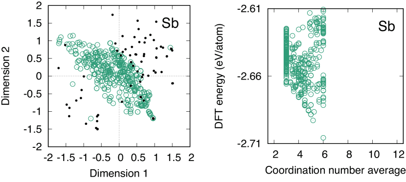
Figure 12: (a) Distribution of the local minimum structures and equilibrium prototype structures in Sb. These structures are mapped into a two-dimensional plane using an MDS. The open and closed circles show the local minimum structures and prototype structures, respectively. (b) Average coordination numbers of the local minimum structures. The cutoff radius is given as 1.2 times the nearest neighbor distance.

In the elemental Sb, 302 structures in the elemental Sb that have relative energy values less than $\theta=$ 75 meV/atom have been discovered. However, for $\theta=15$ and 30 meV/atom, only two and 24 structures have been found, respectively. Figure 12 (a) shows the distribution of the local minimum structures and equilibrium prototype structures in Sb. Most of the local minimum structures are far from the equilibrium prototype structures. Figure 12 (b) shows the distribution of average coordination numbers for the local minimum structures in Sb. The elemental Sb prefers open structures, and the global minimum structure is six-coordinated. The coordination numbers of the local minimum structures range from three to six.

Table 9: Global and local minimum structures in Sb. The DFT relative energy $\Delta E$ is expressed in the unit of meV/atom. $Z$ denotes the number of atoms included in the unitcell.

Space group	ICSD-ID	Prototype	$Z$	$\Delta E$
$R\bar{3}m$	9859	As	6	0.0
$Pm$	$-$	$-$	12	12.9
$R\bar{3}m$	$-$	$-$	36	17.3
$P6_{3}mc$	$-$	$-$	12	17.3
$P\bar{3}m1$	$-$	$-$	8	19.3
$P\bar{3}m1$	$-$	$-$	10	20.1
$R\bar{3}m$	$-$	$-$	30	20.6
$P3m1$	$-$	$-$	10	20.6
$P6_{3}mc$	$-$	$-$	8	23.9
$Imma$	$-$	$-$	24	24.3
$R\bar{3}m$	$-$	$-$	24	24.3
$R\bar{3}m$	$-$	$-$	18	24.4
$R\bar{3}m$	$-$	$-$	24	24.4
$P1$	$-$	$-$	8	24.4
$C2/m$	$-$	$-$	12	24.5
$P1$	$-$	$-$	8	24.6
$R3m$	$-$	$-$	24	24.7
$P\bar{3}m1$	$-$	$-$	8	25.8
$Cmce$	$-$	$-$	24	26.7
$Pmma$	$-$	$-$	10	27.4
$P3m1$	$-$	$-$	12	27.8
$R3m$	$-$	$-$	36	27.9
$Cccm$	$-$	$-$	24	28.1
$C2/m$	$-$	$-$	16	29.4
$P6_{3}mc$	31170	C($P6_{3}mc$)	4	40.0
$Pm\bar{3}m$	43211	SC	1	46.4
$Cmce$	23836	black-P	8	47.2
$Pnma$	165995	MnP	8	51.0

Table 9 provides a list of the local minimum structures observed in the elemental Sb. The global minimum structure is the six-coordinated As-type structure, which is also the experimental structure at low temperatures Barrett et al. (1963); Young (1991). In addition, the coordination numbers for all atoms in the As-type structure are obtained as six, similar to the elemental Bi. Other structures such as the C($P6_{3}mc$)-, SC-, black-P- and MnP-type structures are also identified. The SC-type structure is the only known high-pressure polymorph Vereschchagin and Kabalkina (1965) among these structures. Additionally, the BCC- Aoki et al. (1983), HCP- Vereschchagin and Kabalkina (1965), Sb($mP4$)- Kabalkina et al. (1970), Bi($I4/mcm$)- Schwarz et al. (2003), and Bi(III)-type structures Schwarz et al. (2003) are known as high-pressure polymorphs and have been experimentally observed. Among these structures, the BCC-, HCP-, Sb($mP4$)-, and Bi($I4/mcm$)-type structures are included in the list of local minimum structures obtained using the random structure search using the MLP.

IV.8 Sn

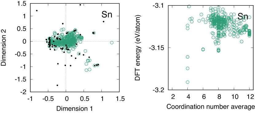
Figure 13: (a) Distribution of the local minimum structures and equilibrium prototype structures in Sn. These structures are mapped into a two-dimensional plane using an MDS. The open and closed circles show the local minimum structures and prototype structures, respectively. (b) Average coordination numbers of the local minimum structures. The cutoff radius is given as 1.2 times the nearest neighbor distance.

There are 310 local minimum structures in the elemental Sn, each with relative energy values lower than $\theta=$ 75 meV/atom. However, only one, four, and thirteen structures are discovered for $\theta=$ 15, 30, and 45 meV/atom, respectively. Figure 13 (a) illustrates the distribution of the local minimum structures and equilibrium prototype structures in Sn. Most of the local minimum structures are located around the equilibrium prototype structures. Figure 13 (b) shows the distribution of average coordination numbers for the local minimum structures in Sn. The global minimum structure and the local minimum structures with low energy values are four-coordinated, while the coordination number of the local minimum structures ranges from four to twelve.

Table 10: Global and local minimum structures in Sn. The DFT relative energy $\Delta E$ is expressed in the unit of meV/atom. $Z$ denotes the number of atoms included in the unitcell.

Space group	ICSD-ID	Prototype	$Z$	$\Delta E$
$Fd\bar{3}m$	28857	Diamond-C($cF8$)	8	0.0
$P6_{3}/mmc$	30101	Wurtzite-ZnS(2H)	4	16.3
$P6_{1}22$	$-$	$-$	6	29.8
$P6_{5}22$	$-$	$-$	6	29.8
$P6/mmm$	52456	Ca.15Sn.85	1	37.0
$Cmmm$	(52456)	(Ca.15Sn.85)	10	37.4
$Cmm2$	(52456)	(Ca.15Sn.85)	22	37.5
$P\bar{3}m1$	(52456)	(Ca.15Sn.85)	3	37.8
$Pmma$	(52456)	(Ca.15Sn.85)	8	37.8
$Pmna$	(52456)	(Ca.15Sn.85)	10	37.8
$P1$	(40037)	($\beta$-Sn)	8	38.4
$Pmc2_{1}$	(40037)	($\beta$-Sn)	8	38.9
$I4_{1}/amd$	40037	$\beta$-Sn	4	39.0
$Fdd2$	$-$	$-$	48	45.6
$Cm$	$-$	$-$	24	46.0
$P2_{1}/c$	$-$	$-$	10	47.6
$I\bar{4}3d$	109012	Li($cI16$)	16	48.0
$I\bar{4}3d$	109012	Li($cI16$)	16	48.0
$C2/c$	$-$	$-$	16	48.9
$C2/m$	$-$	$-$	24	49.8
$Cmce$	89414	Si($oS16$)	16	54.0
$Cm$	(1425)	(HCP)	24	54.8
$Cmcm$	(12174)	(In)	4	56.0
$I4/mmm$	12174	In	2	56.4
	(236711)	(I($Immm$))
$I4/mmm$	24622	Sn($tI2$)	2	56.8
$I4/mmm$	181908	Si($I4/mmm$)	8	67.1
$Pm\bar{3}m$	43211	SC	1	74.2

The local minimum structures in the elemental Sn are listed in Table 10. The global minimum structure is the four-coordinated diamond-type structure, which is the experimental structure at low temperatures Swanson (1953); Young (1991). The local minimum structures also include the wurtzite-, $\beta$-Sn-, Li($cI16$)-, Si($oS16$)-, In-, and Sn($tI2$)-type structures. Experimentally, the $\beta$-Sn- Lee and Raynor (1954); Young (1991), Sn($tI2$)- Barnett et al. (1966), I($Immm$)- Salamat et al. (2013), and BCC-type Salamat et al. (2013) structures have been reported as high-pressure polymorphs, and the $\beta$-Sn-type structure is also known as the high-temperature structure Young (1991). Among these structures, the $\beta$-Sn-, Sn($tI2$)-, and I($Immm$)-type structures are included in the current structure list.

IV.9 Te

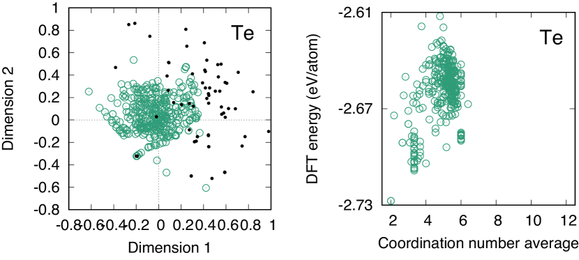
Figure 14: (a) Distribution of the local minimum structures and equilibrium prototype structures in Te. These structures are mapped into a two-dimensional plane using an MDS. The open and closed circles show the local minimum structures and prototype structures, respectively. (b) Average coordination numbers of the local minimum structures. The cutoff radius is given as 1.2 times the nearest neighbor distance.

In the elemental Te, 339 local minimum structures with relative energy values less than $\theta=$ 100 meV/atom have been discovered. On the other hand, only seven structures are discovered for $\theta=$ 20 meV/atom. Figure 14 (a) shows the distribution of the local minimum structures and equilibrium prototype structures in Te. Most of the local minimum structures are far from the equilibrium prototype structures. Figure 14 (b) shows the distribution of average coordination numbers for the local minimum structures in Te. The global minimum structure is two-coordinated, and the coordination numbers of the local minimum structures range from two to six.

Table 11: Global and local minimum structures in Te. The DFT relative energy $\Delta E$ is expressed in the unit of meV/atom. $Z$ denotes the number of atoms included in the unitcell.

Space group	ICSD-ID	Prototype	$Z$	$\Delta E$
$P3_{1}21$	23059	$\gamma$-Se	3	0.0
$P3_{2}21$	653048	Te	3	0.0
$P2$	$-$	$-$	9	18.9
$C2/c$	(23059)	($\gamma$-Se)	12	19.9
$P2_{1}/c$	(23059)	($\gamma$-Se)	12	19.9
$P\bar{1}$	(23059)	($\gamma$-Se)	9	19.9
$C2/c$	(23059)	($\gamma$-Se)	12	20.0
$P2$	$-$	$-$	12	20.7
$R\bar{3}$	27495	S6	18	23.4
$Pm$	$-$	$-$	6	23.8
$P1$	$-$	$-$	12	24.3
$P2_{1}/c$	$-$	$-$	12	24.3
$C2/m$	$-$	$-$	18	24.4
$P2_{1}2_{1}2$	$-$	$-$	6	24.5
$P2$	$-$	$-$	12	24.5
$C2/m$	$-$	$-$	24	25.0
$P2/m$	$-$	$-$	9	26.5
$C2/m$	$-$	$-$	24	27.5
$C2/m$	$-$	$-$	12	28.0
$P1$	$-$	$-$	12	28.4
$C2$	$-$	$-$	18	29.4
$P2/m$	$-$	$-$	9	30.0
$R\bar{3}m$	(43211)	(SC)	3	40.8

Table 11 shows the local minimum structures in the elemental Te. The global minimum structures are the two-coordinated $\gamma$-Se-type chiral structures, which are the experimental structures at low temperatures Bradley (1924); Young (1991). However, most of the local minimum structures do not have assigned prototype structures. In the literature, As- Aoki et al. (1980), Sb₂Te₃- Takumi et al. (2002), GaSb- Vezzoli (1971), Te($mP4$)- Aoki et al. (1980), and Po($hR1$)-types Aoki et al. (1980) are known as high-pressure structures. The first four structures are included in the list of local minimum structures obtained through the random structure search using MLP, showing energy values greater than the threshold.

V Conclusion

This study has developed an efficient iterative procedure that utilizes polynomial MLPs to enumerate both globally stable and metastable structures with high accuracy. The procedure involves updating the MLP and performing a random structure search with the updated MLP. This approach has allowed us to create polynomial MLP models that are both reliable and efficient for structure enumeration. These models are available in the Polynomial Machine Learning Potential repository Mac .

The current procedure has been applied to nine different elemental systems, including As, Bi, Ga, In, La, P, Sb, Sn, and Te. In all of these systems, there are metastable structures that compete with the globally stable structures in terms of energy. This study has shown that it is crucial to exhaustively enumerate metastable structures with low energy values to achieve a robust search for globally stable structures in such systems. By applying the current procedure, the globally stable structures consistent with the experimental structures at low temperatures have been found. Furthermore, many previously unknown metastable structures that compete with the globally stable structures have been discovered, as well as some predicted metastable structures that have prototype structures reported in other systems and experimental structures. Thus, the current procedure will be useful in performing structure searches in more complex systems that have potential energy surfaces with many local minima.