Regularized Benders Decomposition for High Performance Capacity Expansion Models

Abstract

We consider electricity capacity expansion models, which optimize investment and retirement decisions by minimizing both investment and operation costs. In order to provide credible support for planning and policy decisions, these models need to include detailed operations and time-coupling constraints, and allow modeling of discrete planning decisions. Such requirements result in large-scale mixed integer optimization problems that are intractable with off-the-shelf solvers. Hence, practical solution approaches often rely on carefully designed abstraction techniques to find the best compromise between reduced temporal and spatial resolutions and model accuracy. Benders decomposition methods offer scalable approaches to leverage distributed computing resources and enable models with both high resolution and computational performance. Unfortunately, such algorithms are known to suffer from instabilities, resulting in oscillations between extreme planning decisions that slows convergence. In this study, we implement and evaluate several level-set regularization schemes to avoid the selection of extreme planning decisions. Using a large capacity expansion model of the Continental United States with over 70 million variables as a case study, we find that a regularization scheme that selects planning decisions in the interior of the feasible set shows superior performance compared to previously published methods, enabling high-resolution, mixed-integer planning problems with unprecedented computational performance.

I Introduction

As the urgency to mitigate greenhouse gas emissions grows, capacity expansion models (CEMs) play a key role in providing decision support for a sustainable and equitable transition in the electricity sector, helping to avoid misallocation of investment, understand the role of emerging technologies and impact of possible policy interventions, and develop robust strategies to transition to net-zero emissions electricity systems [1, 2, 3, 4]. Ideally, these models should co-optimize generation and transmission investment and retirement decisions across multiple planning periods, and operational dispatch decisions at hourly or finer resolution under different scenarios, with detailed operating constraints (e.g., unit commitment, long duration energy storage), and high geospatial resolution [5]. These requirements result in least-cost optimization problems that combine integer and continuous decision variables subject to a set of linear constraints representing engineering operation and environmental, political, and economic requirements. Integer variables are used to model discrete investment and retirement decisions (and associated economies of scale) across multiple planning periods, which are optimized to minimize capital and operating costs. To estimate operating costs, CEMs include a representation of the underlying electricity system, where continuous variables model dispatch and storage decisions, and linear constraints are used to model physical and operational limits of the considered technologies. The electricity network is modeled as a graph, whose nodes represent different geographical zones. Power flows between zones are represented by a transport model with losses or a linearized optimal power flow model. Typically, each planning period corresponds to one year of system operation, modeled with hourly resolution. Therefore, full resolution CEMs result in large-scale mixed-integer linear programs (MILPs) with tens to hundreds of millions of variables and constraints, pushing even the best commercial solvers to their computational limits. Due to these computational constraints, existing models are heavily simplified by: sampling representative time periods or ignoring sequential operations entirely (e.g., “time slices”); aggregating regions into larger geographic zones; and/or ignoring or relaxing key operational constraints. These abstractions can ensure CEMs are computationally tractable but come at the cost of significantly reduced accuracy that impacts their ability to provide credible decision support [6, 7, 8, 9]. As an example, modelling of long duration energy storage (LDES) resources is becoming central in power system planning, especially when considering the interactions between electricity systems and other energy carriers, or key industrial sectors [5]. However, accurate representation of LDES requires a higher temporal resolution than what is usually considered in capacity expansion models.

As an alternative to abstractions, several studies have focused on developing decomposition methods for solving large optimization problems arising in the framework of energy system planning [10, 11, 12, 13, 14, 15, 16, 17]. A common approach is to implement Benders decomposition to separate planning decisions from operational dispatch decisions. At every iteration, this cutting plane algorithm requires solving two optimization problems: (i) a master problem to select investment and retirement decisions; (ii) a set of operational sub-problems optimizing dispatch decisions over each planning period to generate cuts (linear inequalities) to be added to the master problem. In this standard setting, an operational sub-problem represents a full year of system operation, modeled with hourly resolution, coupled in time by both operational and policy constraints. To reduce the computational cost, some studies do not model integer investment and retirement decisions [10, 11, 16], and simplify the operational model by not considering storage resources [10, 11], or ignoring ramping constraints and unit commitment [10, 11, 14, 15, 16]. In comparison, [12, 13] included detailed operational and time coupling constraints, but then formulated the operational sub-problem only for a selection of representative sub-periods from each year and do not model long-duration energy storage or hydro reservoir resources (which introduce time coupling across operational sub-periods). To further reduce computational burden, studies in [14, 15] propose to avoid solving a full operational sub-problem at every iteration, using inexact cuts based on the approximate solutions of earlier exact iterations. Such approach results in significant computational savings, but it requires the operational sub-problems from different planning periods to have the same constraint matrices, with variations allowed only in the right-hand side of the inequalities. Moreover, the capacity expansion models formulated in [14, 15] consider identical renewables availability profiles across planning periods, as well as the same demand hourly patterns. They represent varying demand across planning periods by applying a scaling factor to the demand hourly profile. This limits their application when considering different weather years (i.e. renewables availability patterns). Further investigations are needed to assess the efficacy of these inexact cuts when variable parameters include hourly demand and renewable availability time series - like the general form in Problem (2).

Moving beyond previous works, [17] presented a model reformulation and solution algorithm for single-period CEMs that allows us to decompose the full operational year into shorter sub-periods. By generating multiple cuts per iteration (one for each operational sub-period), the method accelerates convergence relative to alternative Benders formulations that produce fewer cuts per iteration (one per each planning period) [12, 13, 14, 15, 16]. Moreover, by taking advantage of distributed computing resources to solve the operational sub-problems in parallel, this algorithm significantly reduces the computational cost associated with each iteration compared to other literature. The present study extends the single-period formulation in [17] to the case of multi-period CEMs, which pose additional challenges due to the increased number of master problem decision variables, which grows with the number of considered resources and planning periods. In fact, as shown in Section V, the Benders decomposition algorithm from [17] can suffer from slow convergence due to oscillations between extreme planning decisions. This is a known issue of cutting plane methods, exacerbated by the large-number of planning decision variables included in multi-period CEMs. In continuous optimization, regularization techniques like proximal-bundle [18] and trust region methods [19, 16] methods mitigate this oscillating behavior by controlling the step size at each iteration. However, the presence of discrete investment and retirement decisions complicates the use of proximal penalty terms and trust regions, since integer feasible solutions may be far apart in the decision space. An alternative approach is offered by level-set methods[20][21, Section 3.3.3], which have been successfully applied to regularize cutting plane methods to solve mixed integer optimization problems [22, 23, 15]. In these schemes, each iteration solves a regularization problem selecting a sub-optimal feasible solution of the master problem, with a bound on its level of sub-optimality controlled by a tunable parameter. Compared to proximal-bundle and trust region methods, level-set methods depend on a single parameter, which does not need to be dynamically updated at each iteration [21, Section 3.3.3].

In this manuscript, we extend the formulation in [17] to model multi-period investment and retirement decisions, as well as long-duration energy storage resources. The key contributions of this paper are the implementation of level-set methods to accelerate the Benders decomposition algorithm from [17], making it computationally feasible to extend the method to much larger planning problems (e.g. multi-stage problems,) and the numerical evaluation of different regularization schemes, identifying the most effective technique for this class of problems. Our study goes further than previous literature [10, 11, 12, 13, 14, 15, 17, 16] and demonstrates the benefits of generating Benders cuts by initially implementing a regularized Benders decomposition algorithm to solve a relaxation of the CEM with continuous planning decisions, enforcing integrality constraints only when the continuous relaxation has reached convergence. In this way, we limit the number of iterations solving a master problem with integer variables and also provide good quality valid cuts to warm-start the solution of the original CEM with discrete planning decisions. All methods are numerically evaluated using a capacity expansion model for the continental United States with 26 zones, over a thousand resources, three planning periods, and hourly temporal resolution for 52 weeks in each planning stage (26,208 total operational periods), which result in a CEM with 69 million variables (including 4,626 integer decisions) and 144 million constraints. We compare the regularized decomposition methods with solution algorithms previously proposed by [12, 13, 17] and show superior performance thanks to regularization and the ability to decompose the operational year into parallelized sub-periods, adding multiple Benders cuts at each iteration.

II Multi-period capacity expansion model

This study considers multi-period power system capacity expansion models, where investment and retirement decisions are optimized over multiple planning periods, while also optimizing generation dispatch decisions with hourly resolution. To formulate the model, we utilize the open-source package GenX (v0.3.5), and full model details are available in the documentation [24] and technical report [25]. In the following, we present the model in compact form and highlight its most relevant properties. GenX considers each planning period $p\in P$ as a single operational year modeled with hourly resolution. We subdivide a planning period $p$ into sub-periods $w\in W_{p}$. In this study, a sub-period represents an operational week (i.e., $168$ hours), resulting in $52$ sub-periods (i.e., $8736$ hours) for each period of one year. GenX formulates a multi-period capacity expansion model as a mixed-integer linear program (MILP) with the objective of minimizing total system cost. Integer variables are grouped in index set $I$ and represent generation and storage capacity investment and retirement as well as transmission expansion decisions. We include these planning decision variables in the vector $y_{p}\in Y$ for each period $p\in P$, where :

$$Y=\Big{\{}y\in\mathbb{R}^{n_{y}}_{\geq 0}\;\Big{|}\;y_{i}\in\mathbb{Z},\;\forall i\in I\Big{\}}.$$ (1)

Generator dispatch decisions, storage levels, power flows, and unit commitment decisions are included in the vector of continuous variables $x_{w}\in\mathbb{R}^{n_{x}}$ for each operational sub-period $w\in W_{p}$ (e.g., week). A compact problem formulation is presented in Equation (2).

min $$\sum_{p\in P}\Big{(}f_{p}^{T}y_{p}+\sum_{w\in W_{p}}c_{w}^{T}x_{w}\Big{)}$$ (2a)

s.t. $$A_{w}x_{w}+B_{w}y_{p}\leq b_{w},\quad\forall w\in W_{p},\;p\in P$$ (2b)

$$\sum_{w\in W_{p}}Q_{w}x_{w}\leq e_{p},\quad\forall p\in P$$ (2c)

$$\sum_{p\in P}R_{p}y_{p}\leq r$$ (2d)

$$x_{w}\geq 0,\quad\forall w\in W_{p},\;\forall p\in P$$ (2e)

$$y_{p}\in Y,\quad\forall p\in P$$ (2f)

The objective function (2a) defines total system cost as the sum of fixed costs and variable costs, denoted by vectors $f_{p}$ and $c_{w}$, respectively. Fixed costs include fixed operation and maintenance costs, as well as the cost of investment in new generation and transmission capacity. Variable costs consider fuel prices, variable operation and maintenance costs, and penalties for non-served energy and policy constraint violations. Constraints (2b) consist of all operational constraints that do not couple different sub-periods. These include capacity constraints for all power generation resources, transmission constraints, ramping limits, start-up and shut-down constraints for thermal generators (i.e., unit commitment constraints), as well constraints modeling the operation of storage resources. Policy constraints coupling all sub-periods like CO2 emission limits or Renewable Portfolio Standards (RPS) are included in constraints (2c). Finally, constraints on investment and retirement decisions for different planning periods are grouped in (2d).

In power system modeling, power flow is represented using energy networks, where different buses are connected via transmission lines. Because energy networks with thousands of nodes (i.e. buses) and transmission lines are computationally intractable, CEMs typically aggregate nodes within the same geographical area that have similar demand and climate conditions and between which power flows are rarely constrained. Similarly, we cluster resources within each aggregate node (or zone) based on their location, technology type, cost of connection to the grid, and operational properties. Therefore, power systems are represented by graphs whose nodes correspond to zones with aggregated demand and several aggregated generation and storage resource clusters, and edges model the interzonal transmission constraints, resulting from the aggregation of transmission lines. As observed in [26], the inclusion of power flow equations, e.g., Kirchhoff’s Voltage Law (KVL), has greater impact on models with lower level of aggregation, compared to highly aggregated models. Since the system considered in Section V is a 26-zone model representing the continental United States, we do not to model KVLs when representing transmission between aggregated zones. We instead employ a lossy transport model which includes linearized power losses across interzonal transmission lines - see Equations (15)-(19) in [25]. Note the same methods and formulations discussed in this paper can be applied to models with linearized power flow equations (e.g., KVLs).

Unit commitment constraints are formulated for each thermal resource cluster using the aggregated representation proposed in [6]. As noted by [13], the optimality gap resulting from relaxing the integrality constraints on unit commitment variables is often small in practice, while such relaxation results in significant computational savings. Therefore, we consider continuous unit commitment decision variables. The modeling of unit commitment, ramping limits, and storage operation requires the formulation of time-coupling constraints. CEMs often represents these constraints by using circular-indexing, where the first time step of each sub-period is treated as immediately following the last time step of the sub-period for purposes of time-coupling constraints - see [12, 13, 14, 15, 17]. As an illustrative example, we discuss this formulation for storage constraints. Since we are considering all sub-periods within a planning period, we assume without loss of generality that $W_{p}=\{1,\ldots,|W_{p}|\}$. Let $H_{w}$ be the index set of all hourly time steps included in sub-period $w\in W_{p}$, and define $t^{0}_{w}\in H_{w}$ as the first time step of the sub-period and $t_{w}\in H_{w}$ as the last time step of the sub-period. Variable $x^{soc}_{g,t}$ denotes the component of vector $x_{w}$ corresponding to the state of charge of storage resource $g$ at time $t\in H_{w}$. Analogously, $x^{wdw}_{g,t}$ and $x^{inj}_{g,t}$ correspond to the electricity withdrawn from and injected into the system, respectively, by storage resource $g$ at time $t\in H_{w}$. Parameters $\eta^{self}_{g}$, $\eta^{c}_{g}$, and $\eta^{d}_{g}$ are percentages of self-discharge rate, charging efficiency, and discharging efficiency, respectively. As shown in the Appendix, when circular-indexing is not considered, storage operation is described by the following equations:

$$\begin{split}&x^{soc}_{g,t}=(1-\eta^{self}_{g})x^{soc}_{g,t-1}+\eta^{c}_{g}x^{wdw}_{g,t}-\frac{x^{inj}_{g,t}}{\eta^{d}_{g}}\\ &\forall t\in H_{w}\setminus\{t^{0}_{w}\}\\ &x^{soc}_{g,t^{0}_{w}}=(1-\eta^{self}_{g})z^{soc}_{g,w}+\eta^{c}_{g}x^{wdw}_{g,t^{0}_{w}}-\frac{x^{inj}_{g,t^{0}_{w}}}{\eta^{d}_{g}}\\ &z^{soc}_{g,w}=x^{soc}_{g,t_{w}}-\Delta x^{soc}_{g,w},\end{split}$$ (3)

for all $w\in W_{p}$. In the above equation, $z^{soc}_{g,w}$ and $\Delta x^{soc}_{g,w}$ represent the energy storage level at the start of sub-period $w$ and change in energy storage level during sub-period $w$, respectively, and are governed by:

$$\begin{split}z^{soc}_{g,1}&=z^{soc}_{g,|W_{p}|}+\Delta x^{soc}_{g,|W_{p}|}\\ z^{soc}_{g,w}&=z^{soc}_{g,w-1}+\Delta x^{soc}_{g,w-1},\quad\forall w=2,\ldots,|W_{p}|.\end{split}$$ (4)

The circular-indexing approximation used in [12, 13, 14, 15, 17] assumes that storage levels between sufficiently long sub-periods are decoupled and it sets $\Delta x^{soc}_{w}=0$ in (3) for all $w\in W_{p}$, ignoring (4). As a result, storage constraints corresponding to different sub-periods are independent. In other words, they are are block-diagonal with respect to the sub-period index $w\in W_{p}$, like in constraint (2b). Due to the computational challenges encountered when solving models with full-year resolution, previous studies have often considered only a few sub-periods for each planning period [12, 13, 14, 15]. Such approximation may give rise to errors when sub-periods are too short, as they fail to fully capture electricity demand and variable renewable resources’ availability profiles. These errors are exacerbated when considering only few 24-hour sub-periods (days), as done in [12, 13]. In comparison to these previous studies, here we consider $52$ sub-periods (weeks) for each planning period, each sub-period consisting of $168$ hours. While circular-indexing with weekly sub-periods may not cause significant errors when considering short-duration storage technologies [27], this does not hold for long-duration energy storage resources. As noted in [5], accurately representing long-duration energy storage (LDES) in CEMs is a key requirement to evaluate their role in decarbonized energy systems. Here, we move beyond previous literature [12, 13, 14, 15, 16, 17] and allow sub-period decomposition for CEMs that include LDES constraints (3) and (4). To achieve this, we note that if starting storage level ($z^{soc}_{g,w}$), and change in storage level during each sub-period ($\Delta x^{soc}_{g,w}$) are fixed, storage constraints (3) are decoupled with respect to the sub-period index $w\in W_{p}$. Hence, if we consider these variables as planning decisions and include them in $y_{p}\in Y$, storage constraints have a block-diagonal form like constraints (2). In this way, the method presented in the next section can be applied to CEMs that include LDES constraints to decompose the full operational year into sub-periods, as long as the master problem optimizes investment and retirement decisions, as well as starting storage level and change in storage level in each sub-period. While this approach increases the number of variables in the master problem, only a small number of the storage resources in the system requires LDES modeling, while all others can be modeled with circular-indexing and week-long sub-periods. Hence, we expect the benefits of decomposing the full-operational year into sub-periods to outweigh the modest increase in master problem solving time.

III Benders Decomposition

We consider an equivalent formulation of Problem (2):

min. $$\sum_{p\in P}\Big{(}f_{p}^{T}y_{p}+\sum_{w\in W_{p}}c_{w}^{T}x_{w}\Big{)}$$ (5a)

s.t. $$A_{w}x_{w}+B_{w}y_{p}\leq b_{w},\quad\forall w\in W_{p},\;p\in P$$ (5b)

$$Q_{w}x_{w}\leq q_{w},\quad\forall w\in W_{p},\;p\in P$$ (5c)

$$\sum_{w\in W_{p}}q_{w}\leq e_{p},\quad\forall p\in P$$ (5d)

$$\sum_{p\in P}R_{p}y_{p}\leq r$$ (5e)

$$x_{w}\geq 0,\quad\forall w\in W_{p},\;\forall p\in P,$$ (5f)

$$y_{p}\in Y,\quad\forall p\in P$$ (5g)

where we have introduced budgeting variables $q_{w}$ to ensure that constraints (2c) are equivalent to (5c) and (5d) for every planning period $p\in P$, as shown in [17, Theorem 1]. We implement a Benders decomposition algorithm to solve Problem (5). At iteration $k\geq 0$, given a choice of planning decisions $y^{k}_{p}$ and budgeting variables $q^{k}_{w}$, for each $w\in W_{p}$ and $p\in P$, we solve the operational sub-problem:

$$g^{k}_{w}= c_{w}^{T}x_{w}$$ min (6a)

s.t. $$A_{w}x_{w}+B_{w}y_{p}\leq b_{w}$$ (6b)

$$Q_{w}x_{w}\leq q_{w}$$ (6c)

$$y_{p}=y^{k}_{p},\quad:\pi_{p}^{k}$$ (6d)

$$q_{w}=q^{k}_{w},\quad:\lambda_{w}^{k}$$ (6e)

$$x_{w}\geq 0,$$ (6f)

where $\pi_{p}^{k}$ and $\lambda^{k}_{w}$ are Lagrangian multipliers associated with the corresponding constraints. We define the current best upper bound as:

$$U^{k}=\min_{j=0,\ldots,k}\bigg{(}\sum_{p\in P}\Big{(}f_{p}^{T}y^{j}_{p}+\sum_{w\in W_{p}}g^{j}_{w}\Big{)}\bigg{)}.$$ (7)

Denote by $y$ and $q$ the vectors consisting of $y_{p}$ and $q_{w}$ for all $w\in W_{p}$ and $p\in P$, respectively. We compute the next iterate $y^{k+1}$ and $q^{k+1}$ by solving the master problem:

$$L^{k}= \sum_{p\in P}\Big{(}f_{p}^{T}y_{p}+\sum_{w\in W_{p}}\theta_{w}\Big{)}$$ min (8a)

s.t. $$\theta_{w}\geq g^{j}_{w}+(y_{p}-y_{p}^{j})^{T}\pi_{p}^{j}+(q_{w}-q_{w}^{j})^{T}\lambda_{w}^{j},$$ (8b)

$$\quad\forall j=0,\ldots,k,w\in W_{p},\;p\in P$$

$$\sum_{w\in W_{p}}q_{w}\leq e_{p},\quad\forall p\in P$$ (8c)

$$\sum_{p\in P}R_{p}y_{p}\leq r$$ (8d)

$$y_{p}\in Y,\quad\forall p\in P,$$ (8e)

and proceed to the next iteration. The resulting Benders decomposition algorithm is presented in Algorithm 1:

Algorithm 1 Benders decomposition.

Input: $y_{p}^{0}=0$ and $q_{w}^{0}=0$, for all $w\in W_{p}$, $p\in P$. And set $K_{\max}$ and $\epsilon_{\text{tol}}$.

Output: $y_{p}^{*}$ and $q_{w}^{*}$, for all $w\in W_{p}$, $p\in P$.

for $k=0,\ldots,K_{\max}$ do

     for $p\in P$ do

         for $w\in W_{p}$ do

              Solve operational sub-problem (6).

         end for

     end for

     Compute best upper bound $U^{k}$ as in (7).

     Solve (8) to get $L^{k}$, $y^{k+1}$, and $q^{k+1}$.

     if $(U^{k}-L^{k})/L^{k}\leq\epsilon_{\text{tol}}$ then

         Set $y_{p}^{*}={y}_{p}^{k+1}$, $q_{w}^{*}={q}_{w}^{k+1}$, $\forall w\in W_{p}$, $p\in P$.

         Stop.

     end if

end for

Compared to previous literature, each iteration solves multiple smaller sub-problems (6) formulated over sub-periods of the operational year, adding more Benders cuts per iteration. As shown in [17] this greatly improves convergence compared to solving a full size sub-problem for each planning period, which would add one cut per period at each iteration, as done in [12, 13, 15, 16] - see also the results in Section V. Moreover, the sub-problems can be dealt with in parallel, significantly reducing the cost-per-iteration compared to solving a full size sub-problem. Algorithm 1 extends previous work [17] by considering multi-period investment and retirement decisions, rather than a single-period CEM, as well as LDES resources. Note that we assume that sub-problems (6) are always feasible, for every choice of $y^{k}_{p}$ and $q^{k}_{w}$. This can be achieved by including suitable slack variables and penalty terms. When this is not possible, Algorithm(1) has to include the computation of feasibility cuts to be added to Problem (8) - as example, see [22]. Since this step does not change any property of Algorithm 1, we decided to omit it for ease of presentation.

IV Regularized Benders Decomposition

Algorithm 1 belongs to the class of cutting plane methods [21, Section 3.3.2], and it is expected to suffer from instability. In fact, Algorithm 1 may oscillate between different extreme investment and retirement decisions before being able to make substantial progress towards the solution. This is because the approximated system cost in (8a) may significantly underestimate the operational cost of extreme decisions when the number of cuts (8b) is small compared to the number of variables - as shown in Section V. Here, we discuss the application of level-set methods [20, 21, 15, 22, 23] to regularize Algorithm 1. Let $\Phi(\cdot)$ be a convex function and $\alpha\in(0,1)$. At iteration $k\geq 0$ of the Benders decomposition algorithm, we consider the following regularization problem:

min $$\Phi(y,q)$$ (9a)

s.t. $$\theta_{w}\geq g^{j}_{w}+(y_{p}-y_{p}^{j})^{T}\pi_{p}^{j}+(q_{w}-q_{w}^{j})^{T}\lambda_{w}^{j},$$ (9b)

$$\quad\forall j=0,\ldots,k,w\in W_{p},\;p\in P$$

$$\sum_{w\in W_{p}}q_{w}\leq e_{p},\quad\forall p\in P$$ (9c)

$$\sum_{p\in P}R_{p}y_{p}\leq r$$ (9d)

$$\sum_{p\in P}\Big{(}f_{p}^{T}y_{p}+\sum_{w\in W_{p}}\theta_{w}\Big{)}\leq L^{k}(\alpha)$$ (9e)

$$y_{p}\in Y,\quad\forall p\in P,$$ (9f)

where $L^{k}(\alpha)=L^{k}+\alpha(U^{k}-L^{k})$. In contrast to Algorithm 1, we do not define the next iterate $y^{k+1}$ and $q^{k+1}$, as the solution of Problem (8), but rather as the solution of Problem (9), which selects the best feasible solution according to the criterion $\Phi(\cdot)$, and subject to the level-set constraint (9e) on the approximated system cost.

Algorithm 2 Regularized Benders decomposition.

Input: $y_{p}^{0}=0$ and $q_{w}^{0}=0$, for all $w\in W_{p}$, $p\in P$. And set $K_{\max}$, $\epsilon_{\text{tol}}$, and $\alpha\in(0,1)$.

Output: $y_{p}^{*}$ and $q_{w}^{*}$, for all $w\in W_{p}$, $p\in P$.

for $k=0,\ldots,K_{\max}$ do

     for $p\in P$ do

         for $w\in W_{p}$ do

              Solve operational sub-problem (6).

         end for

     end for

     Compute upper bound $U^{k}$.

     Update cuts in Problem (8) and solve it to get $L^{k}$.

     if $(U^{k}-L^{k})/L^{k}\leq\epsilon_{\text{tol}}$ then

         Set $y_{p}^{*}=y_{p}^{k+1}$, $q_{w}^{*}=q_{w}^{k+1}$, $\forall w\in W_{p}$, $p\in P$.

         Stop.

     else

         Solve (9) to get $y^{k+1}$ and $q^{k+1}$.

     end if

end for

Previous literature have suggested various choices for $\Phi(y,q)$ [20, 21, 22, 23], including:

$$\begin{split}&\Phi^{\ell_{2}}(y,q)=\|y-y^{k}\|^{2}_{2}+\|q-q^{k}\|^{2}_{2}\\ &\Phi^{\ell_{1}}(y,q)=\|y-y^{k}\|_{1}+\|q-q^{k}\|_{1}\\ &\Phi^{\ell_{\infty}}(y,q)=\|y-y^{k}\|_{\infty}+\|q-q^{k}\|_{\infty}.\end{split}$$ (10)

When considering $\Phi^{\ell_{n}}$ for $n\in\{1,2,\infty\}$, Problem (9) selects the set of planning and budgeting decisions that are closest to the current feasible solution, and that reduce the approximated system cost to at most $L^{k}(\alpha)$. However, as reported in Table I, these approaches did not perform well when applied to the large case study considered in Section V.

An alternative method adopted by [15] aims to select solutions that are $\alpha(U^{k}-L^{k})$-suboptimal and belong to the interior of the feasible set of Problem (8). This strategy is frequently used in decomposition algorithms when solving continuous problems [28, 29]. In these cases, an interior solution can be computed by setting $\Phi(y,q)=\Phi^{\text{int}}(y,q)=0$, and solving the resulting feasibility problem with an interior point method. Because integer solutions are not at the center of the feasible set of Problem (8), this scheme is not directly applicable to problems with integrality constraints. For this reason, we design a two-stage method, where we first implement Algorithm 2 with $\Phi=\Phi^{\text{int}}$ to solve the continuous relaxation of Problem (2). Note that, even though they have been computed using continuous planning decisions, the cuts generated by Algorithm 2 do not exclude any integer optimal solution of Problem (2). Therefore, they can be used to warm-start the master problem when solving the original MILP. To recover an integer solution, we apply Algorithm 1 keeping all pre-computed cuts in Problem (8) (which now includes integer constraints as in (1)). The two-stage method is summarized in Algorithm 3.

Algorithm 3 Benders-$\Phi^{\text{int}}$ decomposition.

Stage 1. Apply Algorithm 2 with $\Phi=\Phi^{\text{int}}$ ignoring integrality constraints in (1).

Stage. 2 Apply Algorithm 1 including all integrality constraints and initializing Problem (8) with the cuts computed by Stage 1.

V Results

V-A Case study: Continental United States with 26 zones

We consider a 26-zone representation of the electricity system for the Continental United States with input parameters generated by PowerGenome [30] - see Figure 1. The system has 1004 storage and generation resources, including 408 thermal generator clusters, 431 variable renewable energy clusters, and 68 storage clusters. In addition, the modeled electricity network includes 49 transmission links representing existing power transmission capacity between zones, and 8 candidate links corresponding to possible new connections. Both existing and candidate transmission links are eligible for expansion. We implemented our Benders decomposition algorithms as additional optimization solver options for the open-source package GenX (v0.3.5). The monolithic GenX model includes storage constraints, ramping limits, and unit commitment constraints. Because of the level of zonal aggregation, we adopt a transport model with linear losses to approximate power flow between zones - for a full description of the model constraints, see [24].

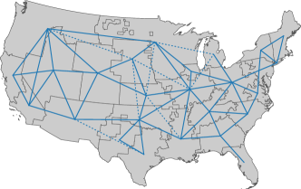
Figure 1: Representation of the Continental United States (CONUS) electricity system with 26 zones. Solid lines correspond to existing transmission capacity between zones, while dotted lines are candidate connections.

We consider transmission and capacity expansion over 3 planning periods (2024-2030, 2031-2040, 2041-2050), with each planning stage represented by a single operational year, with demand corresponding to the final year of the planning stage (to ensure resource adequacy) and investment costs corresponding to the average costs over the planning stage (representing the average cost of a series of capacity additions across the planning stage). An annual CO2 emission constraint is enforced on the operational decisions corresponding to each stage individually. The CO2 cap is set to 186 Mt for 2030, 86.66 Mt for 2040 and 0 Mt for 2050. For the purpose of this study, we also set a CO2 price for violating the emission constraint equal to $150/ton, so that sub-problems (6) are always feasible. System operation is modeled with hourly resolution, and subdivided into 52 sub-periods (i.e. weeks) for each planning period. Therefore, each sub-period includes 168 time steps and the total number of operational time steps is $26,208$. The resulting capacity expansion model is written as Problem (2) with $69,874,284$ variables, $144,752,424$ constraints, and $4,626$ integer variables. Note that the considered model has significantly higher spatial and technological resolution compared to those considered in previous literature [12, 13, 15, 16], resulting in a capacity expansion model that has from 2 to 20 times more variables.

All LPs and MILPs are solved using the solver Gurobi (v.10.0.1) [31], and the GenX model is implemented in Julia (v1.9.1)[32] and JuMP (v1.17)[33]. All LPs are solved with the barrier method. Unless stated otherwise, we set a convergence tolerance of $10^{-3}$ for both Gurobi and the implemented decomposition algorithms. When solving (8) and (9) we deactivate crossover, which is switched on to compute optimal basic primal-dual solutions of the operational sub-problems (6). Note that non-basic dual feasible solutions computed by the barrier method would still provide valid Benders cuts. However, these inexact cuts may not separate the optimal solution from the current primal solution. Hence, the use of inexact cuts may result in increased iterations [34]. Because performing crossover did not require impractical solving times, we use this feature to obtain better quality cuts. The simulations are run on Princeton University’s Della computer cluster.

V-B Benchmarking considering continuous planning decisions

We compare the performance of several decomposition algorithms to solve the continuous relaxation of the multi-period planning Problem (2), where the integrality constraints in (1) are ignored. Algorithm 2, referred to as Benders-$\Phi^{\alpha}$, is implemented with different choices of regularization function $\Phi\in\{\Phi^{\text{int}},\Phi^{\ell_{1}},\Phi^{\ell_{2}},\Phi^{\ell_{\infty}}\}$ and level-set parameter $\alpha\in\{0.2,0.5,0.8\}$. To assess the effect of regularization on the convergence properties of the Benders algorithm, we also evaluate Algorithm 1, referred to as Benders-Base. In addition, we performed benchmarking experiments for algorithms proposed in previous literature. These include the Dual Dynamic Programming (DDP) decomposition algorithm proposed in [12] and previously implemented in GenX (as of v0.3.0), which does not allow any parallel implementation. We also evaluate the approach in [13], decomposing planning stages into year-long operational sub-problems, referred to as Benders-Full. Finally, the trust region scheme with $\ell_{\infty}$-norm from [16], denoted by Benders-TR, is applied as regularization step in Algorithm 2. Because it was observed in [16] that the algorithm performance did not significantly depend on its parameters, we set most parameters as in [16] and only vary the trust region parameter in $\{0.1,0.2,0.3\}$.

All Benders-$\Phi^{\alpha}$, Benders-TR, and Benders-Base experiments reported in this section use a single computing node with 52 cores. This results in 52 parallel processes solving 3 week-long operational sub-problems each. For each choice of $\Phi$, experiments testing different values for the level-set parameters have been performed on the same computing node. Because the decomposition Benders-Full allows to optimize the operations during each year-long planning period independently, we implement it on a single node with 3 parallel processes each using 32 cores (total of 96 cores), while DDP [12] is implemented on a single node with 32 cores (no parallel processes). We set a time limit of 24 hours for each algorithm.

As shown in Table I most algorithms did not converge to a solution within the prescribed time limit. In particular, regularization methods Benders-$\Phi^{\ell_{n},\alpha}$ have reached the time limit with a significant residual optimality gap, larger than $10^{-2}$, for all tested $n\in\{1,2,\infty\}$ and $\alpha\in\{0.2,0.5,0.8\}$. The trust region method Benders-TR did not achieve an optimality gap smaller than $1$ in all instances. As expected, Benders-Full obtained the largest optimality gap at the time limit, being the only tested Benders decomposition method that adds only three cuts at each iteration, solving a year-long operational sub-problem for each planning period. The DDP algorithm from [12] was able to solve the considered model within the time limit of 24 hours, requiring only 3 iterations. However, this approach does not allow parallelization of the sub-problems, limiting its scalability performance with the number of available CPU cores. In contrast to the other distributed approaches, all Benders-$\Phi^{\text{int}}$ implementations were able to reach convergence within the time limit. We believe this can be explained by the ability of the interior point stabilization to select well-centered Benders cuts, yielding quicker progress towards the solution. In particular, Benders-$\Phi^{\text{int},0.5}$ was the fastest algorithm, resulting in a 30% reduction in runtime compared to DDP. To demonstrate the performance of Benders-$\Phi^{\text{int},0.5}$ when able to fully parallelize the solution of the 156 operational sub-problems, rather than being limited to 52 cores, we resolve the model using 6 computing nodes with 26 cores each (total of 156 cores). The regularized Benders algorithm converged to a solution in roughly 6 hours. Thus we observe a $\sim$57% reduction in runtime relative to results reported in Table I, where the algorithm could distribute the sub-problems over only a third of the cores (52 cores). Moreover, the regularized Benders algorithm required $\sim$108 GB of memory compared to the $\sim$368 GB used by the DDP algorithm [12], which can not exploit distributed computing resources as efficiently and performs all computations on a single node. These results indicate we can further increase the number of operational decisions (e.g. additional planning periods or multiple weather and demand scenarios per planning period) while maintaining a runtime shorter than 24 hours, so long as the number of available cores scales proportionately to the number of operational sub-periods considered.

TABLE I: Results for the continuous relaxation of Problem (2).

Method	Iterations	Runtime (hr)	Gap
DDP [12]	3	20	$3.8\times 10^{-4}$
Benders-Full [13]	62	24	8.87
Benders-Base	17	24	1.18
Benders-$\Phi^{\text{int},0.2}$	58	18	9.1$\times 10^{-4}$
Benders-$\Phi^{\text{int},0.5}$	49	14	9.7$\times 10^{-4}$
Benders-$\Phi^{\text{int},0.8}$	65	20	9.8$\times 10^{-4}$
Benders-$\Phi^{\ell_{1},0.2}$	39	24	0.14
Benders-$\Phi^{\ell_{1},0.5}$	38	24	9.7$\times 10^{-2}$
Benders-$\Phi^{\ell_{1},0.8}$	45	24	0.50
Benders-$\Phi^{\ell_{2},0.2}$	36	24	9.7$\times 10^{-2}$
Benders-$\Phi^{\ell_{2},0.5}$	43	24	3.1$\times 10^{-2}$
Benders-$\Phi^{\ell_{2},0.8}$	43	24	1.2$\times 10^{-2}$
Benders-$\Phi^{\ell_{\infty},0.2}$	45	24	0.20
Benders-$\Phi^{\ell_{\infty},0.5}$	38	24	5.4$\times 10^{-2}$
Benders-$\Phi^{\ell_{\infty},0.8}$	109	24	1.72
Benders-TR0.1 [16]	37	24	1.5
Benders-TR0.2 [16]	31	24	1.37
Benders-TR0.3 [16]	34	24	0.84

V-C Modeling discrete planning decisions

When only continuous planning decisions are considered, GenX models transmission expansion as a continuous increase of transmission capacity on the aggregated lines corresponding to the connections shown in Figure1. In comparison, discrete planning decisions explicitly model the number and type of lines that are built on each connection. For each of the 57 inter-zonal connections in Figure1 we consider three line voltages (230kV, 345kV, 500kV) with either single or double circuits, and a 500kV HVDC line, resulting in 7 different line classes. Discrete transmission expansion decisions correspond to the number of new lines from each class, resulting in $57\times 7=399$ transmission expansion integer variables for each planning period. Analogously, discrete generation investment or retirement decisions model the number of units in generation and storage resource clusters that are built or retired. The total number of integer variables in the model is 4,626.

We solve Problem (2) enforcing the integrality constraint in (1) on investment and retirement decisions using Algorithm 3 with $\alpha=0.5$, which is the regularization scheme that performed best in the previous Section. The algorithm is implemented on 156 cores distributed over 6 computing nodes. Recall that Algorithm 3 performs two stages: the first stage ignored integrality constraints and applies the regularized Benders Algorithm 2. The second stage enforces integrality constraints and implements the basic Benders Algorithm 1 initializing the master Problem (8) with the cuts computed at the previous stage. As shown in Figure 2 the pre-initialized master problem at the start of Stage 2 results in a small residual optimality gap ($\sim 1\%$) when integer constraints are taken into consideration. After just four iterations, the optimality gap decreases to below $0.1\%$ reaching convergence. Thus, Algorithm 3 was able to solve the model in just over 6 hours, an unprecedented computational performance for a capacity planning model of this size with discrete planning decisions. This suggests that the proposed regularized Benders algorithm can provide enough computational bandwidth to further reduce model abstractions and approximation errors, for example increasing spatial resolution, or extending the capacity expansion model to include energy sectors beyond electricity (e.g. natural gas, hydrogen) while maintaining a runtime under 24 hours.

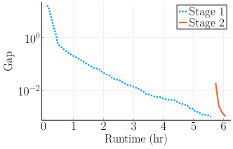
Figure 2: Convergence of Algorithm 3, where Stage 1 solves the continuous relaxation, while Stage 2 enforces the integrality constraints on investment and retirement decisions. Note that the y-axis uses a $\log_{10}$ scale.

The use of discrete decisions helps to capture economies of scale (e.g. lines with higher voltages have lower investment costs), and lumpiness of transmission expansion, encouraging the model to concentrate new investments where they make the biggest impact on electricity generation. Figure 3 reports differences in generation and transmission capacity between models with discrete and continuous investment decisions. In the model with continuous decisions, we assumed a transmission expansion cost per MW equal to the smallest cost between the 7 discrete line options. While total system cost and capacity are relatively similar between the two models, we observe significant regional differences in both transmission and generation capacity. As shown in Figure 3a and Figure 3b, the largest differences in transmission capacity corresponds to areas with significant differences in installed renewable energy generation capacity. This is to be expected as capacity factors of solar and wind generators significantly depends on the availability of sufficient transmission capacity to transfer power from good quality renewable resource zones to demand centers.

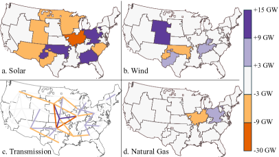
Figure 3: Differences in regional generation and transmission capacity between discrete and continuous decisions cases in 2050. Positive values correspond to increased capacity when discrete decisions are used.

V-D Impact of higher temporal resolution

We compare the solution obtained from a full resolution model with 52 weeks per planning period (and continuous planning decisions), computed by Benders-$\Phi^{\text{int},0.5}$, with those obtained by formulating the GenX model using 41 representative days of operation in each planning period. The representative days are selected using the k-means time domain reduction technique based on [35], which aggregates hourly time series data (e.g., renewable energy availability patterns and demand profiles). Note that this is a common configuration in existing capacity expansion models. As examples, the RIO model [36] is usually set up over a set of representative days (e.g., 41 days in Net Zero America study [37]), while ReEDS [38] models system’s operation with 4 hours (time slices) per season. The Dual Dynamic Programming algorithm implemented in GenX was able to solve the model with 41 representative days in just over 6 hours, a very similar runtime compared to that required by our decomposition algorithm for the full resolution model with 52 weeks - see Figure 2. As shown in Figure 4 the model with 41 representative days overestimates total solar capacity in 2050 by about $15\%$ compared to the full-resolution model. These results are in line with previous literature [35, 39], and indicate that models relying on few representative days may overestimate solar capacity due to the inability to fully capture weekly variability patterns of both renewables and demand. In contrast, our regularized Benders decomposition framework enables full-resolution models with comparable runtime (less than 6 hours), thus mitigating modeling inaccuracies due to temporal aggregation.

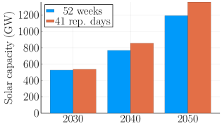
Figure 4: Total solar energy capacity in each planning period, comparing low resolution and high resolution models.

VI Conclusions

We have demonstrated that level-set regularization of Benders decomposition methods combined with a formulation suitable to exploit distributed, parallel computation can offer a scalable approach to solve large-scale, mixed-integer capacity expansion models. For the considered case study with over 70 million variables, our regularized Benders algorithm was able to compute a solution to the continuous relaxation of the planning problem in less than 6 hours and a full solution to the MILP planning problem in just over 6 hours. Key advantages of the proposed algorithm compared to previously published methods include:

1. Ability to further decompose the operational sub-problem into smaller sub-problems, defined over sub-periods of each planning period. This allows to take better advantage of distributed computing resources and to improve convergence by adding more cuts per iteration compared to approaches solving year-long operational sub-problems [12, 13, 15, 16].

2. Generation of better quality Benders cuts using solutions in the interior of the feasible set via level-set regularization, avoiding oscillations and instabilities that affect basic Benders implementations [17].

3. When solving CEMs with integer planning variables, we initialize Benders iterations by loading pre-computed good quality cuts obtained solving a continuous relaxation of the problem. For the considered case study, the Benders algorithm with pre-computed cuts starts from a relatively small optimality gap, and it reaches convergence in just a few additional iterations.

Overall the results are promising and suggest that the regularized Benders decomposition method presented herein can enable capacity expansion models with high computational performance, limiting the role of abstractions which reduce temporal, spatial, and technological resolution and can bias model results. Further research should explore the application of the developed decomposition scheme to stochastic and robust formulations of capacity expansion models, accounting for uncertainty in demand, availability of renewables, and technology costs. Moreover, we note that the proposed method was able to achieve an unprecedented computational performance thanks to available distributed computing resources. In an effort to improve access to high performance capacity expansion models, future work will also focus on the implementation of these techniques on cloud computing infrastructure. Finally macro-scale energy systems planning models representing multiple energy networks and industrial supply chains (e.g., TEMOA [40], RIO [36]) present a very similar problem structure as electricity capacity expansion models. The methods presented herein are therefore extensible to this class of models and others with similar problem structure: e.g., discrete planning or strategic decisions that must be co-optimized with operational or tactical decisions subject to time coupling constraints.

References

- [1] N. A. Sepulveda, J. D. Jenkins, A. Edington, D. S. Mallapragada, and R. K. Lester, “The design space for long-duration energy storage in decarbonized power systems,” Nature Energy, vol. 6, no. 5, pp. 506–516, Mar. 2021. [Online]. Available: https://www.nature.com/articles/s41560-021-00796-8
- [2] M. Victoria, E. Zeyen, and T. Brown, “Speed of technological transformations required in Europe to achieve different climate goals,” Joule, vol. 6, no. 5, pp. 1066–1086, May 2022. [Online]. Available: https://linkinghub.elsevier.com/retrieve/pii/S2542435122001830
- [3] W. Ricks, Q. Xu, and J. D. Jenkins, “Minimizing emissions from grid-based hydrogen production in the United States,” Environmental Research Letters, vol. 18, no. 1, p. 014025, Jan. 2023. [Online]. Available: https://iopscience.iop.org/article/10.1088/1748-9326/acacb5
- [4] J. Bistline, G. Blanford, M. Brown, D. Burtraw, M. Domeshek, J. Farbes, A. Fawcett, A. Hamilton, J. Jenkins, R. Jones, B. King, H. Kolus, J. Larsen, A. Levin, M. Mahajan, C. Marcy, E. Mayfield, J. McFarland, H. McJeon, R. Orvis, N. Patankar, K. Rennert, C. Roney, N. Roy, G. Schivley, D. Steinberg, N. Victor, S. Wenzel, J. Weyant, R. Wiser, M. Yuan, and A. Zhao, “Emissions and energy impacts of the Inflation Reduction Act,” Science, vol. 380, no. 6652, pp. 1324–1327, Jun. 2023. [Online]. Available: https://www.science.org/doi/10.1126/science.adg3781
- [5] T. Levin, J. Bistline, R. Sioshansi, W. J. Cole, J. Kwon, S. P. Burger, G. W. Crabtree, J. D. Jenkins, R. O’Neil, M. Korpås, S. Wogrin, B. F. Hobbs, R. Rosner, V. Srinivasan, and A. Botterud, “Energy storage solutions to decarbonize electricity through enhanced capacity expansion modelling,” Nature Energy, Sep. 2023. [Online]. Available: https://www.nature.com/articles/s41560-023-01340-6
- [6] B. S. Palmintier and M. D. Webster, “Heterogeneous Unit Clustering for Efficient Operational Flexibility Modeling,” IEEE Transactions on Power Systems, vol. 29, no. 3, pp. 1089–1098, May 2014. [Online]. Available: http://ieeexplore.ieee.org/document/6684593/
- [7] K. Poncelet, E. Delarue, D. Six, J. Duerinck, and W. D’haeseleer, “Impact of the level of temporal and operational detail in energy-system planning models,” Applied Energy, vol. 162, pp. 631–643, Jan. 2016. [Online]. Available: https://www.sciencedirect.com/science/article/pii/S0306261915013276
- [8] Q. Xu and B. F. Hobbs, “Value of model enhancements: quantifying the benefit of improved transmission planning models,” IET Generation, Transmission & Distribution, vol. 13, no. 13, pp. 2836–2845, Jul. 2019. [Online]. Available: https://onlinelibrary.wiley.com/doi/10.1049/iet-gtd.2018.6357
- [9] M. M. Frysztacki, J. Hörsch, V. Hagenmeyer, and T. Brown, “The strong effect of network resolution on electricity system models with high shares of wind and solar,” Applied Energy, vol. 291, p. 116726, Jun. 2021. [Online]. Available: https://linkinghub.elsevier.com/retrieve/pii/S0306261921002439
- [10] F. Munoz, B. Hobbs, and J.-P. Watson, “New bounding and decomposition approaches for MILP investment problems: Multi-area transmission and generation planning under policy constraints,” European Journal of Operational Research, vol. 248, no. 3, pp. 888–898, Feb. 2016. [Online]. Available: https://linkinghub.elsevier.com/retrieve/pii/S0377221715007110
- [11] T. Lohmann and S. Rebennack, “Tailored Benders Decomposition for a Long-Term Power Expansion Model with Short-Term Demand Response,” Management Science, vol. 63, no. 6, pp. 2027–2048, Jun. 2017. [Online]. Available: http://pubsonline.informs.org/doi/10.1287/mnsc.2015.2420
- [12] C. L. Lara, D. S. Mallapragada, D. J. Papageorgiou, A. Venkatesh, and I. E. Grossmann, “Deterministic electric power infrastructure planning: Mixed-integer programming model and nested decomposition algorithm,” European Journal of Operational Research, vol. 271, no. 3, pp. 1037–1054, 2018, publisher: Elsevier B.V. [Online]. Available: https://doi.org/10.1016/j.ejor.2018.05.039
- [13] C. Li, A. J. Conejo, P. Liu, B. P. Omell, J. D. Siirola, and I. E. Grossmann, “Mixed-integer linear programming models and algorithms for generation and transmission expansion planning of power systems,” European Journal of Operational Research, vol. 297, no. 3, pp. 1071–1082, 2022, publisher: Elsevier B.V.
- [14] N. Mazzi, A. Grothey, K. McKinnon, and N. Sugishita, “Benders decomposition with adaptive oracles for large scale optimization,” Mathematical Programming Computation, vol. 13, no. 4, pp. 683–703, Dec. 2021. [Online]. Available: https://link.springer.com/10.1007/s12532-020-00197-0
- [15] H. Zhang, I. E. Grossmann, B. R. Knudsen, K. McKinnon, R. G. Nava, and A. Tomasgard, “Integrated investment, retrofit and abandonment planning of energy systems with short-term and long-term uncertainty using enhanced Benders decomposition,” Mar. 2023, arXiv:2303.09927 [math]. [Online]. Available: http://arxiv.org/abs/2303.09927
- [16] L. Göke, Schmidt, Felix, and Kendziorski, Mario, “Stabilized Benders decomposition for energy planning under climate uncertainty,” European Journal of Operational Research, Jan. 2024.
- [17] A. Jacobson, F. Pecci, N. Sepulveda, Q. Xu, and J. Jenkins, “A Computationally Efficient Benders Decomposition for Energy Systems Planning Problems with Detailed Operations and Time-Coupling Constraints,” INFORMS Journal on Optimization, vol. 6, no. 1, pp. 32–45, Jan. 2024. [Online]. Available: https://pubsonline.informs.org/doi/10.1287/ijoo.2023.0005
- [18] A. Frangioni, “Generalized Bundle Methods,” SIAM Journal on Optimization, vol. 13, no. 1, pp. 117–156, Jan. 2002. [Online]. Available: http://epubs.siam.org/doi/10.1137/S1052623498342186
- [19] J. Linderoth and S. Wright, “Decomposition Algorithms for Stochastic Programming on a Computational Grid,” Computational Optimization and Applications, vol. 24, no. 2, pp. 207–250, Feb. 2003. [Online]. Available: https://doi.org/10.1023/A:1021858008222
- [20] C. Lemaréchal, A. Nemirovskii, and Y. Nesterov, “New variants of bundle methods,” Mathematical Programming, vol. 69, no. 1-3, pp. 111–147, Jul. 1995. [Online]. Available: http://link.springer.com/10.1007/BF01585555
- [21] Y. Nesterov, Introductory Lectures on Convex Optimization, ser. Applied Optimization, P. M. Pardalos and D. W. Hearn, Eds. Boston, MA: Springer US, 2004, vol. 87. [Online]. Available: http://link.springer.com/10.1007/978-1-4419-8853-9
- [22] J. Kronqvist, D. E. Bernal, and I. E. Grossmann, “Using regularization and second order information in outer approximation for convex MINLP,” Mathematical Programming, vol. 180, no. 1-2, pp. 285–310, Mar. 2020. [Online]. Available: http://link.springer.com/10.1007/s10107-018-1356-3
- [23] D. E. Bernal, Z. Peng, J. Kronqvist, and I. E. Grossmann, “Alternative regularizations for Outer-Approximation algorithms for convex MINLP,” Journal of Global Optimization, vol. 84, no. 4, pp. 807–842, Dec. 2022. [Online]. Available: https://link.springer.com/10.1007/s10898-022-01178-4
- [24] MIT Energy Initiative and Princeton University ZERO lab, “GenX: a configurable power system capacity expansion model for studying low-carbon energy futures.” [Online]. Available: https://genxproject.github.io/GenX/
- [25] J. D. Jenkins and N. A. Sepulveda, “Enhanced Decision Support for a Changing Electricity Landscape: The GenX Configurable Electricity Resource Capacity Expansion Model,” MIT Energy Initiative, Tech. Rep. MITEI-WP-2017-10, 2017. [Online]. Available: https://hdl.handle.net/1721.1/130589
- [26] F. Neumann, V. Hagenmeyer, and T. Brown, “Assessments of linear power flow and transmission loss approximations in coordinated capacity expansion problems,” Applied Energy, vol. 314, p. 118859, May 2022. [Online]. Available: https://linkinghub.elsevier.com/retrieve/pii/S0306261922002938
- [27] D. S. Mallapragada, N. A. Sepulveda, and J. D. Jenkins, “Long-run system value of battery energy storage in future grids with increasing wind and solar generation,” Applied Energy, vol. 275, p. 115390, Oct. 2020. [Online]. Available: https://linkinghub.elsevier.com/retrieve/pii/S0306261920309028
- [28] J. Gondzio, R. Sarkissian, and J.-P. Vial, “Using an interior point method for the master problem in a decomposition approach,” European Journal of Operational Research, vol. 101, no. 3, pp. 577–587, Sep. 1997. [Online]. Available: https://linkinghub.elsevier.com/retrieve/pii/S0377221796001828
- [29] J. Gondzio, P. González-Brevis, and P. Munari, “New developments in the primal–dual column generation technique,” European Journal of Operational Research, vol. 224, no. 1, pp. 41–51, Jan. 2013. [Online]. Available: https://linkinghub.elsevier.com/retrieve/pii/S0377221712005656
- [30] Greg Schivley, “PowerGenome.” [Online]. Available: https://github.com/PowerGenome/PowerGenome
- [31] Gurobi Optimization, “Gurobi Optimizer 10.1,” 2023. [Online]. Available: https://www.gurobi.com/
- [32] J. Bezanson, A. Edelman, S. Karpinski, and V. B. Shah, “Julia: A fresh approach to numerical computing,” SIAM Review, vol. 59, no. 1, pp. 65–98, 2017, arXiv: 1411.1607.
- [33] M. Lubin, O. Dowson, J. D. Garcia, J. Huchette, B. Legat, and J. P. Vielma, “JuMP 1.0: recent improvements to a modeling language for mathematical optimization,” Mathematical Programming Computation, vol. 15, no. 3, pp. 581–589, Sep. 2023. [Online]. Available: https://link.springer.com/10.1007/s12532-023-00239-3
- [34] G. Zakeri, A. B. Philpott, and D. M. Ryan, “Inexact Cuts in Benders Decomposition,” SIAM Journal on Optimization, vol. 10, no. 3, pp. 643–657, Jan. 2000. [Online]. Available: http://epubs.siam.org/doi/10.1137/S1052623497318700
- [35] D. S. Mallapragada, D. J. Papageorgiou, A. Venkatesh, C. L. Lara, and I. E. Grossmann, “Impact of model resolution on scenario outcomes for electricity sector system expansion,” Energy, vol. 163, pp. 1231–1244, Nov. 2018. [Online]. Available: https://linkinghub.elsevier.com/retrieve/pii/S0360544218315238
- [36] J. H. Williams, R. A. Jones, B. Haley, G. Kwok, J. Hargreaves, J. Farbes, and M. S. Torn, “Carbon-Neutral Pathways for the United States,” AGU Advances, vol. 2, no. 1, p. e2020AV000284, 2021, _eprint: https://onlinelibrary.wiley.com/doi/pdf/10.1029/2020AV000284. [Online]. Available: https://onlinelibrary.wiley.com/doi/abs/10.1029/2020AV000284
- [37] E. Larson, C. Greig, J. Jenkins, E. Mayfield, A. Pascale, C. Zhang, J. Drossman, R. Williams, S. Pacala, R. Socolow, E. Baik, R. Birdsey, R. Duke, R. Jones, B. Haley, E. Leslie, K. Paustian, and A. Swang, “Net Zero America: Potential Pathways, Infrastructure, and Impacts,” Tech. Rep., 2021, annex A.2. [Online]. Available: https://netzeroamerica.princeton.edu/the-report
- [38] J. Ho, J. Becker, M. Brown, P. Brown, I. Chernyakhovskiy, S. Cohen, W. Cole, S. Corcoran, K. Eurek, W. Frazier, P. Gagnon, N. Gates, D. Greer, P. Jadun, S. Khanal, S. Machen, M. Macmillan, T. Mai, M. Mowers, C. Murphy, A. Rose, A. Schleifer, B. Sergi, D. Steinberg, Y. Sun, and E. Zhou, “Regional Energy Deployment System (ReEDS) Model Documentation: Version 2020,” National Renewable Energy Laboratory, Tech. Rep. NREL/TP- 6A20-78195, 2021. [Online]. Available: https://www.nrel.gov/docs/fy21osti/78195.pdf
- [39] J. E. T. Bistline, “The importance of temporal resolution in modeling deep decarbonization of the electric power sector,” Environmental Research Letters, vol. 16, no. 8, p. 084005, Aug. 2021. [Online]. Available: https://iopscience.iop.org/article/10.1088/1748-9326/ac10df
- [40] K. Hunter, S. Sreepathi, and J. F. DeCarolis, “Modeling for insight using Tools for Energy Model Optimization and Analysis (Temoa),” Energy Economics, vol. 40, pp. 339–349, Nov. 2013. [Online]. Available: https://linkinghub.elsevier.com/retrieve/pii/S014098831300159X