Transformer for Times Series: an Application to the S&P500

Abstract

The transformer models have been extensively used with good results in a wide area of machine learning applications including Large Language Models and image generation. Here, we inquire on the applicability of this approach to financial time series. We first describe the dataset construction for two prototypical situations: a mean reverting synthetic Ornstein-Uhlenbeck process on one hand and real S&P500 data on the other hand. Then, we present in detail the proposed Transformer architecture and finally we discuss some encouraging results. For the synthetic data we predict rather accuratly the next move, and for the S&P500 we get some interesting results related to quadratic variation and volatility prediction.

1 Objectives and general introduction

”The transformer models [Vaswani2023], initiated in 2017, have not yet attained maturity in terms of scientific validation and applicability, despite being used in various contexts of machine learning applications including Large Language Models and generative modeling.

Consistent with this general trend, we inquire here about the applicability of this approach to financial time series.

The outline of this work is as follows: we present the general methodology of our approach in Section 2. We then describe the specific neural network model architecture and the choices we made in Section 3. The results on synthetic Ornstein-Uhlenbeck data and on the S&P500 are discussed in Section LABEL:sec:results. The final discussion and conclusions can be found in Section LABEL:sec:conclusion.”

2 Methodology

2.1 First notations and time series embedding

We use the encoder part of a transformer model for time series prediction. From a time series of unidimensional variables $(y_{1},y_{2},\cdots,y_{m})$ we build a probabilistic classifier, which from any partial sequence $(\phi(y_{i})$, $\phi(y_{i+1})$, $\ldots$, $\phi(y_{i+l-1}))$ of length $l$ calculates the probabilities for $y_{i+l}$ to belong to each interval of a fixed interval list; these intervals will be referred to as ”buckets” hereafter. Here, $\phi(.)$ is an embedding function from ${\bf R}$ into ${\bf R}^{d}$ which will be discussed later. Transformers are highly efficient in large language models, where $y_{i}$ represents words (or tokens) and $\phi(y_{i})$ denotes their encodings in a $d$-dimensional space. The value $d$ is called the dimension of the model and is often set to $512$ or $1024$. Here, to achieve dimension $d$, the undimensional variables $y_{i}$ are encoded into some new variables $x_{i}=\phi(y_{i})$ with $\phi(y_{i})=(y_{i},\frac{y_{i}^{2}}{2},\cdots,\frac{y_{i}^{d}}{d!})$. We also incorporate the possibility of including a positional encoding to the process. Different values for $d$ can be chosen, but in our base case we take $d=\frac{l}{2}$. Details regarding positional encoding are provided later in the paper.

Ideally, the conditional laws $\mathcal{L}(Y_{n+l}|(X_{n},X_{n+1},\cdots,X_{n+l-1}))$ should converge as $n$ increases for the model to perform well. To investigate this property, we first utilize simulated data, for which these conditional laws indeed have a limit. Here, the synthetic dataset is simulated from a mean reverting Ornstein-Uhlenbeck process, which involves observable variables $y_{i}$ and hidden state variables $h_{i}$. We assess the performance of the model by comparing its results to the values derived from $\mathcal{L}(Y_{n+l}|\mathcal{F}_{n+l-1})$. Here, $\mathcal{F}_{n+l-1}$ contains all the variables (observable or hidden) up to time $n+l-1$, providing the best possible estimator. Hence, in our simulations, $\mathcal{F}_{n+l-1}$ encompasses not only the knowledge of the $(x_{i})_{i\leq n+l-1}$ but also includes the hidden variables $(h_{i})_{i\leq n+l-1}$. Subsequently, we test the method on market data with the S&P500, initially predicting the next day return and then the next day quadratic variation from which avolatilyt prediction could derive.

2.2 Creating a dataset from a single time series

We observe a single time series $(y_{i})_{i\in\llbracket 1,m\rrbracket}$. To ease notations, we denote $[x]_{i}=(x_{i},x_{i+1},\cdots,x_{i+l-1})$ a sequence of length $l$. Recall that $x$ is a notation for $\phi(y)$.

From the observation of $y$ and their embedding $x$, there are different types of datasets of sequences that can be constructed to train the model:

1. a single dataset of non-overlapping sequences $[x]_{1}$ to predict $y_{l+1}$, $[x]_{l+1}$ to predict $y_{2l+1}$ and so on

2. a single dataset of overlapping sequences $[x]_{1},[x]_{2},\ldots,[x]_{m-l}$ with the corresponding values to predict $y_{l+1},y_{l+2},\ldots y_{m}$

3. $l$ datasets $D_{1},D_{2}..D_{l}$ of non overlapping sequences. Then, classifiers can be calibrated on each of these datasets and combined with an ensemble method. In our case we would have:
   $D_{1}=\{[x]_{1},[x]_{l+1},\cdots\}$
   $D_{2}=\{[x]_{2},[x]_{l+2},\cdots\}$
   $\vdots$
   $D_{l}=\{[x]_{l},[x]_{2l},\cdots\}$.

4. A bootstrap method to build, as in method 3, several datasets made of sequences $[x]_{i}$ where each $[x]_{i}$ is picked at random from the dataset of all sequences, and then apply an ensemble method to this ensemble of datasets.

Here, we use method 2 and split the dataset of sequences into $\{[x]_{1},[x]_{2},\cdots[x]_{m_{1}}\}$ for training and $\{[x]_{m_{1}+1},[x]_{m_{1}+2}\cdots[x]_{m-l}\}$ for testing.

2.3 Ornstein Uhlenbeck process for the $y_{i}$

A time series $(y_{1},y_{2},\cdots,y_{m})$ is generated from some hidden variables $h_{i}$, in the following way :

$$\left\{\begin{tabular}[]{c}$h_{0}\sim\nu_{0}$\\ $\forall n\in{\bf N},h_{n+1}=h_{n}+\theta(\mu-h_{n})dt+\sigma\sqrt{dt}\epsilon_{n+1}\mbox{ with }\epsilon_{n+1}\sim N(0,1)$\\ $y_{n+1}=h_{n+1}-h_{n}$\end{tabular}\right.$$ (1)

We use $\theta>0$ to get a stationary process for the $(y_{i})_{i\in{\bf N}}$ and take in our simulations $\mu=0$, $dt=1$, $\sigma=1$ and $\theta=1$.

As only one trajectory is modeled (see Figure 2), we choose arbitrarily $h_{0}=0$ and from there, the hidden values $(h_{1},h_{2},\cdots h_{m})$ are simulated as well as the $(y_{1},y_{2},...y_{m})$. Note that, the various sequences extracted from this time series with method 2 do not have identical distributions, as each of them is associated to a different initial hidden value $h_{0},h_{1},h_{2}\cdots$ etc. This being said, as we can calculate explicitely $\mathcal{L}(Y_{n+l}|\mathcal{F}_{n+l-1})=\mathcal{L}(Y_{n+l}|H_{n+l-1})$ it is not an issue to evaluate the performance of the model by comparing it to the best possible classifier, which is obtained by calculating the probabilities knowing all the variables observed and hidden at the previous time step. The variables used are recapitulated in Figure 1.

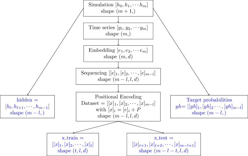
Figure 1: Example of variables used in the simulations.

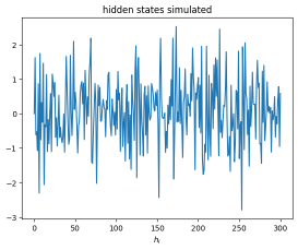
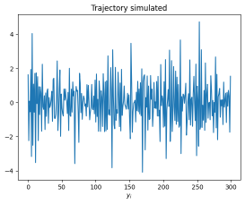
Figure 2: Trajectory of the process (1) for the parameters $dt=1$, $\theta=1$, $\sigma=1$, $\mu=0$. Left: first 301 hidden values $h_{0},...,h_{300}$. Right: first 300 values $y_{1},...,y_{300}$.

2.4 Positional encoding

As a common practice for transformer models, we enable the model to integrate positional encoding. The positional encoding has the same dimension as the model. So, for a sequence $[x]_{i}$ of shape $(l,d)$ the positional encoding will be a matrix $P\in{\bf R}^{l\times d}$. The positional encoding could be be learned, but we use here the standard method with sinusoidal functions. For this method, it is better to have an even number for $d$, which will be the case here.
For $j\in[0,\frac{d}{2}-1]$ we define

$$w_{j}=\frac{1}{10000^{\frac{2j}{d}}}$$

and for $t\in[0,d-1]$, the column vector $p_{t}$ of $P$ is defined as:

$$\left\{\begin{tabular}[]{c}$p_{t,2j}=sin(tw_{j})$\\ $p_{t,2j+1}=cos(tw_{j})$\end{tabular}\right.$$ (2)

This positional encoding presents several interesting properties.

Property 1.

For $k\in[0,d-1]$ let $T_{k}$ be the $2\times 2$ block diagonal matrix such that, $\forall j\in[0,\frac{d}{2}-1],$ each of its $2\times 2$ diagonal block $M_{k}(j)$ is defined by:

$$M_{k}(j)=\begin{bmatrix}cos(kw_{j})&sin(kw_{j})\\ -sin(kw_{j})&cos(kw_{j})\\ \end{bmatrix}$$

then,

1. $\forall k\in[0,d-1],T_{k}$ is an orthonormal matrix. i.e $T_{k}T^{\perp}_{k}=T^{\perp}_{k}T_{k}=Id_{d}$

2. $T_{k+t}=T_{k}T_{t}$

3. $\forall t\in[0,d-1],\|p_{t}\|^{2}=\frac{d}{2}$

4. $p_{t+k}=T_{k}p_{t}$

5. for all vector columns $p_{t}$ and $p_{t+k}$ of $P$ the quantity $\langle p_{t},p_{t+k}\rangle$ only depends on $k$ and is maximum for $k=0$.

6. $\exists$ a function $\psi$ such that $PP^{\perp}=[\psi(|i-j|)]$

Proof.

1. simple calculation as $cos^{2}(kw_{j})+sin^{2}(kw_{j})=1$

2. demonstration block by block using the properties of the trigonometric functions

3. simple using that $sin^{2}+cos^{2}=1$

4. demonstration block by block

   $$M_{k}(j)\begin{pmatrix}p_{t,2j}\\ p_{t,2j+1}\\ \end{pmatrix}=\begin{bmatrix}cos(kw_{j})&sin(kw_{j})\\ -sin(kw_{j})&cos(kw_{j})\\ \end{bmatrix}\begin{pmatrix}sin(tw_{j})\\ cos(tw_{j})\\ \end{pmatrix}=\begin{pmatrix}sin((k+t)w_{j})\\ cos((k+t)w_{j})\\ \end{pmatrix}$$

   which proves the result.

5. $\langle p_{t},p_{t+k}\rangle=\langle p_{t+k},p_{t}\rangle=p_{0}^{\perp}T^{\perp}_{t+k}T_{k}p_{0}=p_{0}^{\perp}T_{k}T^{\perp}_{t}T_{t}p_{0}=p_{0}^{\perp}T_{k}p_{0}$ which only depends on $k$ and $\langle p_{t},p_{t}\rangle=\frac{d}{2}$ while by Cauchy Schwartz $|\langle p_{t},p_{t+k}\rangle|=|p_{0}^{\perp}T_{k}p_{0}|\leq\|p_{0}\|\|T_{k}p_{0}\|=\|p_{0}\|\|p_{0}\|=\frac{d}{2}$ Q.E.D.

6. This result is a consequence of the previous result.

∎

Property 6 implies that the positional encoding enables, by calculating a scalar product between the positional vectors $p_{s}$ and $p_{t}$, to get a notion of time elapsed between time $s$ and $t$.

2.5 The Transformer model for classification

After defining some buckets $B_{1},B_{2},B_{k}$ the objective of the model is, for a sequence $(x_{m+1},x_{m+2},\cdots,x_{m+l})$, to estimate the probabilities $(p_{1},p_{2},\cdots,p_{k})$ for $y_{m+l+1}$ (resp $y^{2}_{m+l+1}$ for quadratic prediction) to belong to these buckets. In the base case, we take the number of buckets to be equal to $7$ obtaining the list $]-\infty,\alpha_{1}],]\alpha_{1},\alpha_{2}],\cdots,]\alpha_{6},+\infty[$ with the $\alpha_{i}$ corresponding to the quantiles of the observed $y_{i}$ (resp $y^{2}_{i}$) from the training set. Therefore, each bucket contains the same proportion of $y_{i}$ (resp $y^{2}_{i}$), up to the rounding errors, from the training set.

The model used is the encoder part of a Transformer, which is a natural choice when solving a classification problem, and we extend the Encoder with some dense layers at the end for the classification task. We call:

• $l$ the length of the sequences $(x_{1},x_{2},\cdots,x_{l})$ used for each prediction. In the base case, $l=32$.

• $d$ the dimension of the model, which is the dimension of each element $x_{i}$, or equivalently the number of features for each $x_{i}$. In the base case here, $d=\frac{l}{2}=16$.

• $k$ the number of buckets used for classification. In the base case here, $k=7$.

• $p$ the proportion of sequences of the dataset used for training. In the base case here, $p=80\%$ and the training sequences use the first observations in chronological order.

In the learning phase, for parameters estimation, the sequences are processed by batches. The default number for a batch is $32$. It is possible to change the batch size in model.fit. Here, in our base case, we take the batch size to be $64$. Below is an example of python code that sets the parameters of the model :

⬇

1model.fit(

2x_train,

3yh_train,

4validation_split=0.2,

5epochs=30,

6batch_size=64,

7callbacks=my_callbacks

The model is built as a sequence of the following blocks :

1. a block to create a) the dataset of the $[x]_{i}$ of shape (Nb of sequences,$l$,$d$), with the positional encoding taken into account as an option and b) the dataset of the $y_{i}$, to be predicted, of shape (Nb of sequences,$l$,$1$). The dataset is split into a training set and a test set and for each $x_{i}$ we can associate the corresponding $h_{i}$ and calculate $\mathcal{L}(Y_{i+1}|H_{i}=h_{i})$.

2. an Encoder block made of a MultiHead Attention block and a Position-wise Feed-Forward block

3. a ”Special Purpose” block for class prediction, once the sequences have been ”contextualised” by the Encoder.

The successive neural layers implemented in Python TensorFlow and Keras are represented in Figure 3 and their functioning is explained below. We explain in details below the functioning of each layer.

Figure 3: Structure of the program.

3 Neural network model details

3.1 Analysis of the different layers

1. The Input tensor defines the shape of an input sequence (instance). It appears as a tensor of shape $(None,l,d)$ ”None” being related to the batch size, which is not explicited in the input tensor construction.

   ⬇

   1inputs=keras.Input(shape=(32,16))\end{lstlisting}

   2

   3

   4

   5

   6

   7

   8\item The \textbf{MultiHeadAttention Layer} produces output tensors of the same shape ($l$,$d$) as the inputs.

   9\begin{lstlisting}[language=Python]

   10x = layers.MultiHeadAttention(key_dim=head_size, num_heads=num_heads, dropout=dropout) (x, x)\end{lstlisting}

   11

   12

   13 \begin{itemize}

   14 \item This layer is explained in more details in the next section. It has two arguments. The first argument is the instance used to calculate the Query and the second argument is the instance used to calculate the Key and the Value. In the Encoder part of a Transformer these two arguments are the same. The head\_size is the dimension chosen for the Queries, Keys and Values. In the original paper "Attention is All You Need" by Vaswani and all, the dimension of the model is 512, the number of heads is 8 and the head\_size is 512/8=64. Here, we keep the 64 for the head\_size. For the dropout, we do not use the dropout layer optionality offered by the Keras MultiHead Attention Layer but, implement it separately. Therefore, we use "dropout=0" and add the following layer.

   15

   16 \item A Dropout Layer

   17\begin{lstlisting}[language=Python]

   18x = layers.Dropout(dropout)(x)\end{lstlisting}

   19 The dropout layer has no learnable parameters and simply transforms any input instance of shape ($l$,$d$) by replacing some units by zero in the training phase (while keeping them identical when predicting). The purpose of the dropout layer is to create some robustness when learning the parameters of the model. We take dropout=0.25.

   20 \end{itemize}

   21

   22\item An Additive Layer

   23\begin{lstlisting}[language=Python]

   24res = x + inputs\end{lstlisting}

   25This layer has no learnable parameters and adds each unit of the dropout layer’s output instance $ (xd_1,xd_2,\cdots, xd_l)$ to each unit of an input instance $(x_1,x_2,\cdots,x_l)$.

   26$$ \mbox{input} + \mbox{dropout layer’s output} \longrightarrow (xd_1+ x_1,xd_2+x_2,\cdots, xd_l+ x_l)$$

   27so, it produces a tensor of shape (None, $l$,$d$).

   28

   29 There is no learnable parameter here.

   30

   31\item A Normalisation Layer (see Tensorflow \cite{TFNL})

   32\begin{lstlisting}[language=Python]

   33x = layers.LayerNormalization(axis=-1,epsilon=1e-6)(res)\end{lstlisting}

   34Layer normalisation is done independently for each sequence (contrarily to batch normalisation), by normalizing along a single axis or multiple axis. So, the mean and variance calculated along this/these axis become respectively zero and 1. By default, Keras normalizes along the last axis. In a transformer the normalization is done along the feature axis (see \cite{Hinton2016}, \cite{Lan2020}), i.e the dimension of the model. So, as the input tensor of the layer is of shape $(None,l,d)$ by saying "axis=-1" (or "axis=2") the normalisation is done in the dimension $d$ as usual.

   35

   36

   37

   38 So, if $x_i \in \R^d$ is the ith element of a sequence (instance) and $x_i^j$ is the value of its feature $j\in [1,d]$, $x_i$ is first transformed into

   39 $$\tilde{x}_i=\frac{1}{\sigma(x_i)+ \epsilon}(x_i- \mu(x_i)1_d)$$

   40

   41 with $\mu(x_i) =\frac{1}{d} \sum\limits_{j=1}^d x_i^j$ and $\sigma(x_i) =\sqrt{\frac{1}{d} \sum\limits_{j=1}^d (x_i^j-\mu(x_i))^2}$

   42

   43The (small) arbitrary parameter $\epsilon$ is chosen to insure that no division by zero occurs. So, each $\tilde{x}_i$ of a sequence gets normalized features in $\R^d$ of expectation $0$ and variance 1.

   44

   45 The second thing that the normalization layer does is an affine transformation for the axis which has been normalized.

   46 Here, the normalization occurs over [axis=-1] of shape ($d$) so, the shapes of the scale-tensor $\gamma$ and center-tensor $\beta$ are ($d$). The $\tilde{x}_i^j$ are transformed by these learnable tensors $\beta=(\beta_1,\beta_2, \cdots \beta_d )$ and $\gamma=(\gamma_1,\gamma_2, \cdots\gamma_d )$ in the following way.

   47

   48$$ \tilde{x}_i^j \longrightarrow \gamma_j \tilde{x}_i^j + \beta_j $$

   49The number of learnable parameters is $2d$.

   50

   51Then comes the Position-wise Feed Forward block with:

   52

   53\item A 1D Convolution Layer (see Keras \cite{TFConv1D}).

   54\begin{lstlisting}[language=Python]

   55x = layers.Conv1D(filters=ff_dim, kernel_size=1, activation="relu")(x)\end{lstlisting}

   56Each filter corresponds to a transformation which is affine if "use bias= True" (which is the default) and otherwise linear.

   57Here, the shape of the input tensor is $(None,l,d)$ and each affine transformation is done along "axis=1".

   58As "kernel size=1", the transformation is done one $x_i$ at a time.

   59$$x_i \longrightarrow w_i^{\prime}x_i +b_i $$ with $w_i$ and $b_i$ learnable of shape $(l)$.

   60The output tensor is of shape (None, $l$, ff\_dim).

   61In Vaswani \cite{Vaswani2023} ff\_dim $= 4\times d$ and the activation function is "relu". We use here the same multiplier $4$, and the same activation function. The number of learnable parameters is $(d+1)\times l \times $ ff\_dim.

   62

   63

   64\item A Dropout Layer

   65\begin{lstlisting}[language=Python]

   66x = layers.Dropout(dropout)(x)\end{lstlisting}

   67\item Another 1D Convolution Layer, but this time with a number of filters equal to $d$ to produce an output of shape ($l$,$d$).

   68\begin{lstlisting}[language=Python]

   69x = layers.Conv1D(filters=inputs.shape[-1], kernel_size=1)(x)\end{lstlisting}

   70

   71This layer finishes the Position-wise Feed Forward block. Then comes,

   72

   73\item An Additive Layer

   74\begin{lstlisting}[language=Python]

   75res = x + inputs\end{lstlisting}

   76\item A Normalization Layer

   77\begin{lstlisting}[language=Python]

   78x = layers.LayerNormalization(axis=-1,epsilon=1e-6)(inputs)\end{lstlisting}

   79

   80This Encoder Block is iterated 6 times in Vaswani \cite{Vaswani2023}. This is also what we do in our base case by defining

   81"num transformer blocks=6".

   82

   83Note that our program performs better when the last Normalization Layer 9 is moved in front of the Multihead Layer and it is what we do in our base case as indicated by the red arrow in Figure \ref{fig:blocks}.

   84

   85

   86The last part of the model is specific to our classification objective and its input tensor of shape (None,$l$,$d$) must be transformed into a tensor of shape (None, $l$,$k$). This last block is made of the following layers.

   87

   88

   89\item A GlobalAveragePooling1D layer. \\

   90\begin{lstlisting}[language=Python]

   91x = layers.GlobalAveragePooling1D(data_format="channels_first")(x)\end{lstlisting}

   92By default the average is done along the sequence axis, transforming an input tensor of shape $(None,l,d)$ into an output tensor of shape $(None,d)$.

   93Here, the model performs better when the average is done along the features (channels) axis.

   94By adding the argument ’’data\_format="channels\_first"’ the layer treat the input tensor as if its shape was $(None, d,l)$ therefore calculating the averages along the last axis. Therefore, with this argument in our model the output tensor has the shape $(None,l)$.

   95

   96

   97\item A Dense Layer with a number of neurons equal to "mlp units".

   98We take in our base case "mlp units =[10]" and implement a single layer with no iteration. To implement a succession of $p$ Dense Layers, the number of units of these successive layers are entered as a numpy array "mlp units = $[n_1, n_2,....n_p]"$.

   99\begin{lstlisting}[language=Python]

   100x = layers.Dense(dim, activation="relu")(x)\end{lstlisting}

   101

   102\item A Dropout Layer

   103\begin{lstlisting}[language=Python]

   104x = layers.Dropout(mlp_dropout)(x)\end{lstlisting}

   105in our base case we take mlp\_dropout$=0.25$.

   106\item A final Dense Layer which produces an output of shape $($n\_classes,$)$ i.e $(7,)$.

   107\begin{lstlisting}[language=Python]

   108outputs = layers.Dense(n_classes, activation="softmax")(x) \end{lstlisting}

   109

   110% https://colab.research.google.com/drive/1zcpITqF0cEcs03VGEbaImKqe-IDHi8cA#scrollTo=aZ7Nv2Eyq4XV

   111

   112\end{enumerate}

   113

   114The model is implemented with Python tensorflows on Google Colab (Python torch is also popular alternative).

   115

   116\subsection{The Multi Head Transformer-Encoder}

   117

   118

   119The different layers of the MultiHead Transformer-Encoder are described in more details here:

   120 \begin{enumerate}

   121

   122

   123

   124

   125\item a MultiHead Attention Layer. This block produces output tensors of the same shape as the input tensors.

   126$$(None, l, d) \longrightarrow (None, l, d) $$

   127The operations conducted are as follows

   128\begin{itemize}

   129\item each Head transforms an input tensor of shape $(None, l,d)$ into a tensor of shape $(None,l,d_v)$ via the Attention Mechanism

   130\item these $nb_{heads}$ tensors are then concatenated to form a tensor of shape $(None, l,nb_{heads} \times d_v) $

   131\item then a linear layer transforms this tensor into a tensor of shape $(None, l, d)$

   132\end{itemize}

   133

   134The MultiHead Attention Mechanism works as follows:\\

   135For each "Head", each observation $x_i$ of shape $(d,)$ is transformed linearly according to some learnable matrices \\

   136$W_K$ of dim $(d,d_k)$ to produce a Key-tensor $x_i^K= x_i W_K$ of shape $(d_k,)$ \\

   137$W_Q$ of dim $(d,d_k)$ to produce a Query-tensor $x_i^Q= x_i W_Q$ of shape $(d_k,)$\\

   138$W_V$ of dim $(d,d_v)$ to produce a Value-tensor $x_i^V= x_i W_V $ of shape $(d_v,)$.\\

   139

   140We call

   141$K =\begin{pmatrix}

   142 x_1^K \\

   143 \vdots \\

   144 x_l^K \\

   145\end{pmatrix}$,

   146$Q =\begin{pmatrix}

   147 x_1^Q \\

   148 \vdots \\

   149 x_l^Q \\

   150\end{pmatrix}$,

   151$V =\begin{pmatrix}

   152 x_1^V \\

   153 \vdots \\

   154 x_l^V \\

   155\end{pmatrix}$

   156

   157These matrices are of respective dimensions $(l,d_k)$, $(l,d_k)$, $(l,d_v)$.

   158

   159We call Attention Matrix $A$ the matrix of dimension $(l,l)$ defined as: \\

   160$$ A = softMax\Big(\frac{1}{\sqrt{k}}QK^{\perp}\Big)$$

   161The softmax function is applied line by line so that the sum of each line of $A$ is one and then we calculate the quantity

   162$$ AV$$

   163Thus, we obtain for each Head a matrix $AV $ of dimension $(l,d_v)$ which are concatenated to form a matrix

   164$\begin{pmatrix}

   165 z_1\\

   166 \vdots \\

   167 z_l \\

   168\end{pmatrix}$ of dimension $(l,nb_{heads} \times d_v)$.

   169

   170Last step is to use a learnable matrix $W_O$ of shape $(nb_{heads} \times d_v,d)$ to transform $z$ into

   171$V =\begin{pmatrix}

   172 z_1W_O \\

   173 \vdots \\

   174 z_lW_O \\

   175\end{pmatrix}$ of shape $(l,d)$.

   176

   177

   178

   179

   180 \end{enumerate}

   181

   182\subsection{Performance of the model}

   183

   184 \subsubsection{Crossentropy}

   185The cross entropy between a target probability $P=(p_1,p_2,\cdots, p_k)$ of belonging to the $k$ buckets and a softmax prediction $Q=(q_1,q_2,\cdots, q_k)$ is defined as:

   186

   187$$ H(P,Q)=-\sum\limits_{j=1}^k p_j ln(q_j) \geq H(P,P)$$

   188

   189and $\min\limits_{Q} H(P,Q)$ is reached for $Q=P$.

   190

   191In the learning phase, the cross entropy is minimised between the dirac probabilities $P_i=(1_{B_1}(y_{i+l}),1_{B_2}(y_{i+l}),\cdots, 1_{B_k}(y_{i+l}) )$ observed and the probabilities $Q_i=(q^i_1,q^i_2,\cdots, q^i_k)$ predicted from the observation $[x]_i$. For a batch, made of $\# B$ sequences, the loss function minimised is :

   192

   193$$\frac{1}{\# B} \sum\limits_{i \in B} H(P_i,Q_i)$$

   194

   195With simulated data we can calculate the target probabilities $T_i$ based on all events (hidden and observable) occured up to time $i+l-1$ as

   196$$t^i_j=P(y_{i+l} \in B_j | H_{i+l-1}=h_{i+l-1})$$

   197

   198

   199

   200

   201\subsubsection{Categorical accuracy}

   202The categorical accuracy provides another measure of performance by measuring the percentage of correct bucket predictions (the bucket predicted for $y_{i+1}$ is the one maximising the $q^i_j$ for $j \in \llbracket 1,k\rrbracket$).

   203

   204There are $k$ buckets. At the beginning, the model does not know how to use the $[x]_i$ to predict and makes prediction at random and therefore predicts correctly in $\frac{1}{k}$ of the cases and we observe and accuracy of $\frac{1}{k}= \frac{1}{7}= 14.28\%$.

   205

   206 After training with the simulated data, the accuracy approaches $30\%$, which is not far from the best possible accuracy derived with the $T_i$.

   207

   208 Indeed, the best possible accuracy for bucket prediction is reached when the target probabilities $T_i$ are used and when the predicted bucket is defined as $$ \arg\max\limits_{j} t_j^i $$

   209 with this method, the Categorical Accuracy reached from the sample of 24131 observations is $31.85\%$ on the train set and $32.00\%$ on the test set.

   210

   211

   212

   213

   214

   215\subsubsection{Pointwise analysis of the predictions }

   216With simulated data, we can calculate the target probabilities $T_i$ based on all variables (hidden and observable) occured up to time $i+l-1$ as

   217$$t^i_j=P(y_{i+l} \in B_j | H_{i+l-1}=h_{i+l-1})$$ that the classifier should ideally be able to approximate, and compare the quantities $H(T_i,Q_i) $ to our targets $H(T_i,T_i) $. The comparison is done by calculating the average of these two quantities on the train set and on the test set.

   218

   219When the model starts training it does not know how to use past observations and therefore find a probability $Q$ independent of the $[x]_i$ which solves

   220$$ \min\limits_{Q} -\sum\limits_{i=1}^k \frac{1}{k}ln(q_i) $$ Therefore, the solution is, $\forall i \in \llbracket 1,k \rrbracket, q_i= \frac{1}{k}= \frac{1}{7}$ which results in a loss function equal to $ln(k)=ln(7)=1.9459$, which is what we get at the beginning of the optimisation process. As the optimisation progress, we expect the loss function to get closer to

   221$$\underset{i}{Average} \{ H(T_i,T_i)\} \sim 1.63 $$

   222

   223and we manage to get pretty close.

   224

   225

   226

   227

   228For each $[x]_i$ we compare the probabilities $Q_i$ predicted by the model to the target probabilities $T_i$ by plotting for each bucket $j \in \llbracket 1,k \rrbracket$ the points $(h_{i+l-1},q^i_j)$ and the points $(h_{i+l-1},t^i_j)$, see Figure \ref{fig:example1} and Figure \ref{fig:example2}.

   229

   230\subsection{Parameters of the model}

   231

   232We make the arbitrary choice in our base model to work with sequences of length 32.

   233The big difference between NLP and times series is that for time series there is no standard method to embed numbers. We choose here an arbitrary function $\phi$ for embedding.

   234Note that, when we calculate in the Multihead Attention block the scalar products $\langle \phi(x_i) ,\phi(x_j)\rangle $ the choice of $\phi$ creates some Kernel $K(x_i,x_j)=\langle \phi(x_i) ,\phi(x_j)\rangle $ which generally speaking are important tools in classification and prediction problems.

   235

   236

   237\begin{table}[h]

   238 \centering

   239 \begin{tabular}{|>{\centering\arraybackslash}m{6cm}|>{\centering\arraybackslash}m{5cm}|}

   240 \hline

   241 Base case NLP encoder & Base case time series prediction \\

   242 \hline

   243 length sequence: $l \sim 1024$ & $l=32$ \\

   244 \hline

   245 embedding dimension: $d=512 $ & $d=\frac{l}{2}=16$ \\

   246 \hline

   247 Positional Encoding: sinus and cosinus & sinus and cosinus \\

   248 \hline

   249 number of heads: $h =8$ & $h=8$ \\

   250 \hline

   251 head size: $d_k =\frac{d}{N_h}=64$ & $d_k = 64$ \\

   252 \hline

   253 number of block iterations: $N=6$ & $N=6$ \\

   254 \hline

   255 number of units FFN: $d_{ff}= 4\times d = 2048 $ & $d_{ff}= 4\times 16= 64 $ \\

   256 \hline \hline

   257 & Dense layer classifier $mlp\_units = [10]$ \\

   258 \hline

   259 \end{tabular}

   260 \caption{Parameters of the model.}

   261 \label{tab:exemple1}

   262\end{table}

   263

   264

   265The model uses, the categorical cross entropy for the loss function, Adam for the optimizer and the "categorical accuracy" for the metrics.

   266

   267

   268\begin{lstlisting}[language=Python]

   269model.compile( loss="categorical_crossentropy",

   270optimizer=keras.optimizers.Adam(learning_rate=1e-3),

   271metrics=["categorical_accuracy"])\end{lstlisting}

   272

   273

   274We use 80\% of the times series for learning and 20\% for test. In the learning phase the model uses 80\% of the learning sequences for calibration and 20\% for validation.

   275

   276\section{Results} \label{sec:results}

   277

   278

   279

   280\subsection{Prediction mean reverting Ornstein-Uhlenbeck synthetic data}

   281

   282We present here some results obtained in our base model; the parameters, inspired by the base model of Vaswani \& Al \cite{Vaswani2023}, are given in Table \ref{tab:exemple1}.

   283

   284We considered here a trajectory of the synthetic

   285stochastic process~\eqref{eq:ouprocess} with

   286$24131$ data points, the same as the number of daily data we will use for the prediction on the S\&P500 market index. The results are given in Table \ref{tab:example2}.

   287\begin{table}[h]

   288 \centering

   289 \begin{tabular}{|p{1.1cm}|p{1.7cm}|p{1.9cm}|p{1.9cm}|p{1.5cm}|p{1.5cm}|}

   290 \hline

   291 Number of epochs & Number of observations & Train~set: Loss~$H(P,Q)$, Accuracy&

   292 Test~set: Loss~$H(P,Q)$, Accuracy & Train~set $H(P,T)$, $H(T,T)$ & Test~set $H(P,T)$, $H(T,T)$ \\

   293 \hline

   294 30 & 24131 & 1,681 & 1.697 & 1.626 & 1.636 \\

   295 & & 30.33\% & 28.66\% & 1.630 & 1.628 \\

   296 \hline

   297 30 & 241310 & 1,656 & 1.656 & 1.631 & 1.630 \\

   298 & & 30.60\% & 30.74\% & 1.631 & 1.629 \\

   299 \hline

   300 40 & 241310 & 1,657 & 1.657 & 1.631 & 1.630 \\

   301 & & 30.56\% & 30.77\% & 1.631 & 1.629 \\

   302 \hline

   303 \end{tabular}

   304 \caption{Analysis of the results obtained with simulated data.}

   305 \label{tab:example2}

   306\end{table}

   307

   308We se that the model enables accurate prediction of the bucket probabilities (the blue points correspond to the perfect probability predictions with the $T_i$) but a significant number of instances are needed to train it.

   309

   310\begin{figure}[htbp!]

   311\centering

   312\includegraphics[width=1.\textwidth]{21455.png}

   313\caption{Predictions for the synthetic

   314 stochastic process~\eqref{eq:ouprocess} with 24131 observations, 30 epochs.}

   315\label{fig:example1}

   316\end{figure}

   317

   318

   319

   320\begin{figure}[htbp!]

   321 \centering

   322 \includegraphics[width=1.\textwidth]{214550epoch40}

   323 \caption{Predictions for the synthetic

   324 stochastic process~\eqref{eq:ouprocess} with 241310 observations, 40 epochs.}

   325 \label{fig:example2}

   326\end{figure}

   327

   328

   329\subsection{Prediction on the S\&P500 Index}

   330

   331We now make predictions on market data using the closing prices for the S\&P500 Index from the $30^{th}$ December 1927 to the $1^{th}$ February 2024.

   332We dispose of 24131 price observations.

   333Here, the variables $h_i$ correspond to the logarithm $ln(p_i)$ of the prices observed and we build predictions for the

   334\begin{equation} y_i = ln(p_i)- ln(p_{i-1}) \end{equation} which are the daily log returns observed (see Figure \ref{fig:trajectory2}).

   335

   336In the first program we predict the bucket for $y_i$, i.e, we try to guess the probability distribution of the daily log return for the next business day.

   337In the second program we predict the bucket for $y_{i}^2$ (the quadratic variation of the log prices) for the next business day.

   338

   339

   340

   341\begin{figure}[htbp!]

   342 \centering

   343 \includegraphics[width=0.49\textwidth]{SP_Log_process.pdf}

   344 \includegraphics[width=0.49\textwidth]{SP_daily_returns.pdf}

   345 \caption{{\bf Left:} Log prices of the S\&P500 over the period.

   346 {\bf Right:} first 300 daily log returns $y_1, ...,y_{300}$.}

   347 \label{fig:trajectory2}

   348\end{figure}

   349

   350

   351

   352

   353

   354

   355

   356

   357

   358\subsection{Prediction of the next return $y_i$}

   359

   360When we applied the base model it became stuck in predicting constant bucket probabilities, without differentiating between the $[x]_i$ (see Figure \ref{fig:example5}).

   361We used $10$ epochs and for all $i$ in the train set the probability predictions for the $k=7$ buckets (defined by the

   362quantiles $a_j$, $j=1,...,k-1$ as described earlier) were all equal to :

   363$$\{0.14200473, 0.14268069, 0.14331234, 0.1455955, 0.1445429, 0.1425599, 0.1393042\}$$

   364As all are equal, this means that the model is failing to make an interesting prediction because it fails to take into account the conditional information $[x]_i$.

   365

   366We did not spend too much efforts trying to improve these predictions, for which we had limited hopes, and directed our efforts towards the $y_i^2$ prediction objective.

   367

   368\begin{figure}

   369\centering

   370\includegraphics[width=1.\textwidth]{SP_testset.png}

   371\caption{bucket predictions for $y_{i+l}$ on the test set for the S\&P500.}

   372\label{fig:example5}

   373\end{figure}

   374

   375

   376\subsection{Prediction of the next quadratic variation $y_{i+l}^2$}

   377

   378Here, the aim is from an observed $[x]_i$, to predict the bucket for $y_{i+l}^2$. This is the first step to predict the gamma cost of hedging options and future volatility. As statistical studies using GARCH models for example have advocated for some degree of predictibility, we expect that our predictions will surpass random chance in this case.

   379

   380

   381The model parameters remain the same as before and we continue to refrain from positional encoding, which appears to hinder learning. Fifty epochs seem to be enough to calibrate and we get the following results.

   382

   383\begin{table}[h]

   384 \centering

   385 \begin{tabular}{|p{1.7cm}|p{2cm}|p{2.2cm}|p{2.2cm}|}

   386 \hline

   387 Number of & Number of & Train set & Test set \\

   388 epochs & observations & Loss $H(P,Q)$ & Loss $H(P,Q)$ \\

   389 & & Accuracy & Accuracy \\

   390 \hline

   391 50 & 24131 & 1,861 & 1.876 \\

   392 & & 21.92\% & 22.84\% \\

   393

   394 \hline

   395 \end{tabular}

   396 \caption{bucket predictions for $y_i^2$.}

   397 \label{tab:example}

   398\end{table}

   399

   400

   401

   402The predicted probabilities for the $k=7$ buckets, corresponding to the successive sequences $[x]_i$ in the test set, are illustrated in Figure \ref{fig:quadratic}. While the results are imperfect, they surpass those of a random prediction across the $k$ buckets (which are equally likely in the training set), yielding a cross-entropy of $\ln(k)=\ln(7)=1.9459$ and an accuracy of $\frac{1}{k}=\frac{1}{7}=14.28\%$.

   403

   404Another natural benchmark for evaluating our classifier is the "naive" classifier, which assigns $y_{i+l}^2$ (with 100\% probability) to the same bucket as $\frac{1}{l} \sum\limits_{j=i}^{j=i+l-1}y_j^2$. For this classifier, the accuracy on the test set is $19.27\%$, and the predicted classes for the successive $[x]_i$ are depicted in Figure \ref{fig:naive}. Once again, our classifier outperforms this naive approach, which is an encouraging outcome.

   405

   406Undoubtedly, there is room for further refinement to enhance the performance of the Encoder Classifier. This could involve adjustments to the structure, choice of encoding method, model dimensionality, inclusion of additional variables, and so forth. Nonetheless, we view this current work as a promising starting point, yielding some encouraging results.

   407

   408

   409

   410

   411

   412\begin{figure}

   413 \centering

   414 \includegraphics[width=1.\textwidth]{quadratic_SP.png}

   415 \caption{bucket predictions for $y_{i+l}^2$ on the test set for the S\&P500.}

   416 \label{fig:quadratic}

   417\end{figure}

   418

   419\begin{figure}

   420 \centering

   421 \includegraphics[width=1.\textwidth]{naive.png}

   422 \caption{Naive classifier for $y_{i+l}^2$ on the test set for the S\&P500.}

   423 \label{fig:naive}

   424\end{figure}

   425

   426

   427

   428

   429

   430

   431\section{Conclusion} \label{sec:conclusion}.

   432

   433

   434In this study, we applied a transformer encoder architecture to times series prediction. The significant differences from LLM applications of transformers is that here we are dealing with numerical data (of dimension 1) and not tokens embedded in spaces of dimension 512 or 1024 (with a specific logic behind the embedding process). We felt compelled to embed the numbers into a higher dimension space in order to prevent significant information loss in the normalization layers (that encoders possess). That being said, our approach to embedding numbers is rather naive and just based on the premise that by embedding numbers with a function $\phi$ the scalar product we create in the process $\langle \phi(x_i), \phi(x_j)\rangle$ may be related to some useful Kernel $K(x_i,x_j)= \langle \phi(x_i), \phi(x_j)\rangle$. We did not have to do too much fine tuning to have a working model in the simulation case, whose results were therefore encouraging. However, we were surprised to find that positional encoding did not enhance prediction accuracy or improve convergence speed. Additionally, we noticed that altering the value of $\theta$ in the simulations could degrade model performance or impede learning, necessitating adjustments. The main differences between our structure and the standard encoder is the normalization layer that we put before the multi-head instead of before the classifier block. This deviation was motivated by the recommendation against normalizing before a dense classification layer. Regarding the prediction of the square of the daily returns of the S\&P500, which can be useful in terms of volatility and cost of gamma hedging predictions, we find the results encouraging. However, we believe that the model’s performance could be further improved through more fine-tuning of the transformer’s structure, as well as the embedding process and selection of additional observation variables.

   435

   436

   437

   438\begin{thebibliography}{9}

   439

   440\bibitem{Zeng} Ailing Zeng, Muxi Chen, Lei Zhang, Qiang Xu.

   441 (2023) \emph{Are Transformers Effective for Times Series Forecasting?} The Thirty-Seventh AAAI Conference on Artificial Intelligence, 2023 (AAAI-23).

   442

   443\bibitem{Vaswani2023}

   444Ashish Vaswani, Noam Shazeer, Niki Parmar, Jakob Uszkoreit, Llion Jones, Aidan N. Gomez, Lukasz Kaiser, Illia Polosukhin, (2017) \emph{Attention Is All You Need}, arXiv:1706.03762v7, 2 August 2023.

   445

   446\bibitem{TFConv1D} Conv1D layer,

   447 \url{https://keras.io/api/layers/convolution_layers/convolution1d/}, retrieved Feb. 29th 2024

   448

   449\bibitem{Eli}

   450Eli Simhayev, Kashif Rasul, Niels Rogge, (2023) \emph{Yes, Transformers are Effective for Time Series Forecasting (+ Autoformer)}, \url{https://huggingface.co/blog/}, 16 June 2023.

   451

   452\bibitem{Hinton2016}

   453Jimmy Lei Ba, Jamie Ryan Kiros, Geoffrey E.Hinton, (2016) \emph{Layer Normalization}, arXiv:1607.06450v1, 21 July 2016.

   454

   455

   456\bibitem{Wen} Qingsong Wen, Tian Zu, Chaoli Zhang, Weiqi Chen, Ziqing Ma, Junchi Yan, Liang Sun.

   457 (2023) \emph{Transformers in Times Series: A Survey}, Proceedings of the Thirty-Second International Joint Conference on Artificial Intelligence (IJCAI-23).

   458

   459

   460\bibitem{Lan2020}

   461Ruibin Xiong, Yunchang Yang, Di He, Kai Zheng, Shuxin Zheng, Chen Xing, Huishuai Zhang, Yanyan Lan, Liwei Wang, Tie-Yan Liu, (2020) \emph{On Layer Normalization in the Transformer Architecture}, arXiv:2002.04745v2, 29 June 2020.

   462

   463

   464

   465\bibitem{TFNL} TensorFlow v2.15.0.post1, (2024) \url{https://www.tensorflow.org/api_docs/python/tf/keras/layers/LayerNormalization}, last updated 2024-01-11 UTC.

   466

   467

   468

   469

   470

   471

   472

   473

   474\end{thebibliography}

   475

   476

   477

   478

   479

   480

   481

   482\end{document}’