Proposed high order harmonic interferometer
for aperture synthesis radio telescope:
Theory and computer simulation

Abstract

A new type of interferometer, called High Order Harmonic Interferometer (HOHI), was proposed by Wu [1996] for imaging by aperture synthesis radio telescope. Its feasibility was proven by theoretical analysis. Before putting HOHI in practical use, computer simulation is a necessary intermediate stage. In this paper the theoretical analysis is reviewed. Then, computer simulation, including its algorithm, calculation and generated maps, is presented. The theoretical analysis is validated by studying these maps.

keywords. aperture synthesis radio telescope – instrumentation: interferometers – high order harmonic interferometer – computer simulation

1 Introduction

In an aperture synthesis radio telescope (ASRT), a correlator is used for each baseline to generate a Fourier component of the radio map, that is, the distribution of power density (brightness) of the field of view (FOV) in the sky under observation. The map is reconstructed by the Fourier transform (FT) technique.

The resolvability of an ASRT depends mainly on the maximum baseline. Therefore, conventionally the increase of resolvability is achieved by extending the maximum baseline. A new technique was proposed by Wu [1996], in which the increase of resolvability was achieved by using a new type of interferometer, called the High Order Harmonic Interferometer (HOHI), without extending the maximum baseline.

This paper is devoted particularly to the HOHI of second order. Its theory is reviewed first. For completeness, some mathematical formulas and a figure in Wu [1996] are reproduced, mutatis mutandis. Then, computer simulation is presented, including its algorithm, calculation and generated maps. These maps are studied in detail and the theory of HOHI is validated. Some practical issues in the implementation of HOHI are discussed.

2 Theory of HOHI

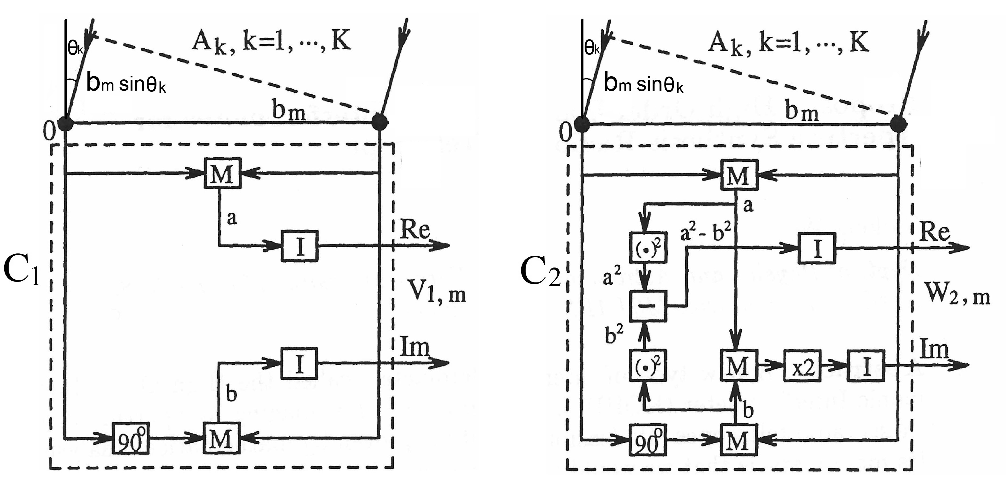
Figure 1: Correlators for the baseline $b_{m}$.   $\mathrm{C}_{1}$: Conventional (base).  $\mathrm{C}_{2}$: Second order. [Wu, 1996]

In the following, one-dimensional (1-D) notation is used for simplicity and clarity. As depicted in Fig. 1 , $\mathrm{C}_{1}$ and $\mathrm{C}_{2}$ are respectively the conventional (base or first harmonic) correlator and the second harmonic correlator, where $b_{m}$ ($m=1,...,M$) is a baseline, $b_{M}$ being its maximum; the block M is multiplier, I is integrator (time averager), and the $90^{\mathrm{o}}$ block is phase shifter.

Suppose in the FOV there are $K$ point sources having amplitudes $A_{k}$ and random phases $\phi_{k},\,k=1,...,K$. The radiations of wavelength $\lambda$ from a single point source $A_{k}$ arrive at the angle $\theta_{k}$ with respect to the normal to the baseline. Then, the phase difference is $2\pi u_{m}x_{k}$ between the two signals in the left and right branches for the baseline $b_{m}$, where $u_{m}=b_{m}/\lambda$ (baseline measured in wavelengths), and the coordinate $x_{k}=\sin\theta_{k}$ (instead of $\theta_{k}$) is used to specify the angular position of point source $k$.

The output from $\mathrm{C}_{1}$ is

$$V_{1,m}=W_{1,m}=\frac{1}{2}\sum_{k=1}^{K}A_{k}^{2}\mathrm{e}^{-i2\pi u_{m}x_{k}}\;.$$ (1)

Here $i=\sqrt{-1}$. $V_{1,m}$ is the (complex) visibility output from the conventional interferometer (the spatial frequency being $1\times u_{m}=u_{m}$). The output from $\mathrm{C}_{2}$ is

$$W_{2,m}=\frac{1}{4}\left\{\sum_{k=1}^{K}A_{k}^{4}\mathrm{e}^{-i2\pi 2u_{m}x_{k}}+4\sum_{p=1}^{K}\sum_{q>p}^{K}A_{p}^{2}A_{q}^{2}\mathrm{e}^{-i2\pi u_{m}(x_{p}+x_{q})}\right\}\;,$$ (2)

which consists of the desirable second harmonics and unwanted cross terms. The latter can be eliminated by operations as shown in the following:

$$V_{2,m}=2V_{1,m}^{2}-W_{2,m}=\frac{1}{4}\sum_{k=1}^{K}A_{k}^{4}\mathrm{e}^{-i2\pi 2u_{m}x_{k}}\;.$$ (3)

$V_{2,m}$ is the visibility output for the baseline $b_{m}$ from the HOHI of second order. Its spatial frequency is $2u_{m}$, that is to say, every baseline is virtually increased by a factor of 2. In particular, let $m=M$, the maximum baseline, $b_{M}$, is virtually doubled. Therefore, the resolvability of the telescope is also doubled.

3 Computer simulation of HOHI

The purpose of computer simulation is to generate 1-D maps using visibilities $V_{1,m},m=1,...,M$ from the conventional interferometer (called base) and $V_{2,m},m=1,...,M$ from the HOHI of second order (called 2nd-order). A number of cases are studied. In each case the base map is compared with the 2nd-order map.

Our “virtual” ASRT has an east-west antenna array with the following parameters: wavelength $\lambda=0.21$ meter, the number of baselines (channels) $M=144$, the baseline increment $d=4.286$ meters, and the maximum baseline $b_{M}=617.184$ meters. They are taken from the synthesis telescope at Dominion Radio Astrophysical Observatory (DRAO, Landecker et al. 2000) .

The visibility used to reconstruct maps has $L=2M+1=144\times 2+1=289$ data points, where the factor $2$ accounts for the Hermitian property of visibility (each $V_{1,m}$ or $V_{2,m}$ from the interferometers has its complex conjugate); the additional $1$ accounts for the zero-baseline component. If this visibility is used for the FT without zero-padding, the pixel size $\Delta x$ of the map would be $\lambda/d/L=0.21/4.286/289=1.6954\times 10^{-4}$. This pixel size is called unit (pure number). In order to increase the accuracy of measurement, zero-padding to the visibility must be used to interpolate the generated maps, that is, to reduce the pixel sizes of maps. These reduced pixel sizes will be expressed in terms of unit.

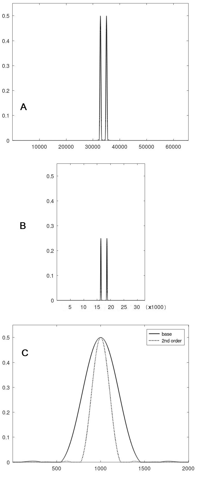
Figure 2: Case 1. Maps of two well-resolved point sources. A. Base. FT length=65536. B. 2nd-order. FT length=32768. C. Left peaks in the central parts of A (solid line) and B (dotted line). Length=2001.

Simulation is carried out using the Octave language [Eaton et al., 2022]. Four cases are studied. They are: 1. Two point sources are located far apart so that they are well resolved in both the base and 2nd-order maps. 2. Two point sources are located closely such that they are not resolved in the base map but resolved in the 2nd-order map. 3. Two point sources are located so closely that they are not resolved in either the base or 2nd-order maps. 4. An extended source.

3.1 Case 1. Two point sources, well resolved

The purposes of this study are to calculate the Full Widths at Half Maximum (FWHMs) in the base and 2nd-order maps, and to compare them.

Two point sources have the same amplitude of 1.0 and are located at 0 unit (at the center of the FOV, $x=0,\,\theta=0$ radian) and 10.0 units, respectively. This sufficiently large distance between the two sources ensures that they are well resolved in the reconstructed maps.

First of all, we determine the necessary FT length, $L_{1}$, for the base map to ensure the accuracy of measurement. The measurement of FWHM we implement using Octave has the maximum error of two pixels. The required measurement accuracy is $0.01$ unit. Therefore, in the worst case we have $2\times 289/L_{1}=0.01$, and $L_{1}=2\times 289/0.01=57800$. For the most efficient Fast Fourier Transform (FFT), this number is run up to a power of 2, and we get $L_{1}=65536=2^{16}$. Correspondingly, the accuracy is $2\times 289/65536=0.0088$ that is better than $0.01$. On the other hand, in comparison with the base map, the 2nd-order map has effectively the doubled maximum baseline and hence a halved pixel size. As a result, the required FT length is $L_{2}=L_{1}/2=2^{15}=32768$.

For generating the base map, the visibilities $V_{1,m},m=1,...M$ calculated using Eq. 1 and their complex conjugates are used as the positive and negative parts of the FT components, respectively. The zero-baseline visibility (total power) is unavailable, but we know that it will be greater than the absolute values of other visibilities. Therefore, the maximum of the absolute values of $V_{1,m},m=1,...M$ will be taken as the zero-baseline visibility, that is, the zero-frequency component. By the way, this component will determine the background of the reconstructed map, but will not affect the resolvability.

The resultant $2M+1$ point visibility is tapered by the Hanning window, and then zero-padded to obtain the required FFT length. Finally, the FFT is performed to generate the map.

Shown in Fig. 2  are three maps. A. Base map. It is reconstructed using the base visibility as described in the preceding paragraphs. The FT length is $65536$. The map center is at $32769$. B. 2nd-order map. It is generated in the same way as generating A, except that the visibilities $V_{2,m},m=1,...M$ calculated using Eq. 3 are used and the FFT length is $32768$. The map center is at $16385$. These two maps have the same pixel size $0.0044$ unit.

In the HOHI of second order all the baselines, including the maximum baseline, are stretched by a factor of 2. Meanwhile, the baseline increment (sampling interval) is also increased by a factor of 2. Therefore, the resolvability is doubled while the width of synthesized field (WSF) is halved. Specifically, for the base map $d=4.286$ meters, and the $\mathrm{WSF}=\lambda/d=0.21/4.286=0.0490$. In contrast, for the 2nd-order map the $\mathrm{WSF}=\lambda/(2d)=0.0245$. This is why the horizontal axis length of map B is a half of that of map $\bf A$.

As expected, the images of the point sources have peak values $0.5$ and $0.25$ in maps A and B, respectively. Furthermore, the images in map B have narrower peaks compared with the images in map $\bf A$. This means that the resolvability in map B is better. This improvement of resolvability can be seen clearly in map C.

Shown in map C are the left peaks in the central parts of maps A (solid line) and B (dotted line). Note that the latter has been scaled for pixel values so its maximum is equal to that of the former for the ease of visual comparison and calculation. Quantitatively, the FWHMs of the 2 peaks are $451$ and $225$ pixels, respectively. Their ratio is $451/225=2.00$, that is, the resolvability of the 2nd-order map is improved by a factor of 2.

3.2 Case 2. Two point sources, located closely

The purpose of this study is to visually show that in the critical case the resolvability in the base map and that in the 2nd-order map are dramatically different.

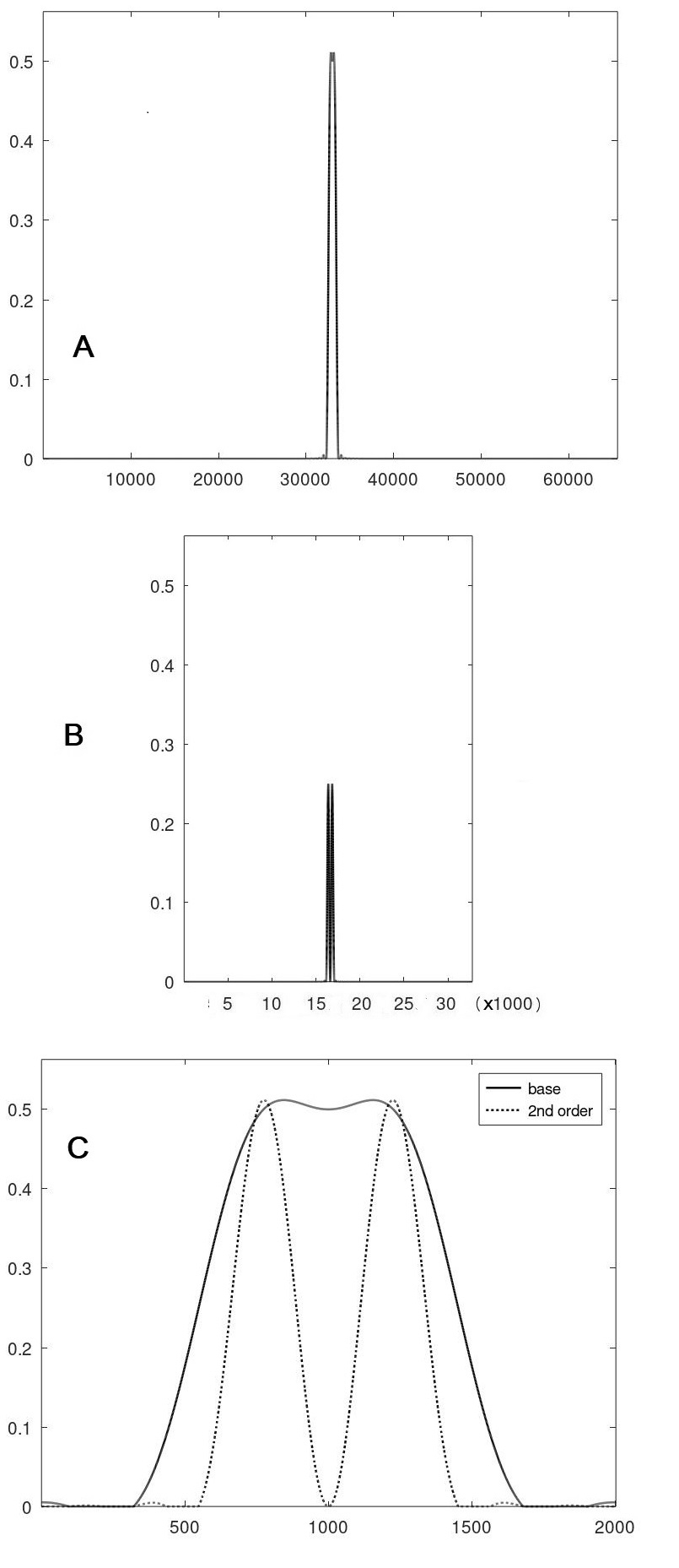
Figure 3: Case 2. Maps of two closely-located point sources. A. Base. FT length=65536. B. 2nd-order. FT length=32768. C. The central parts of A (solid line) and B (dotted line). Length=2001.

Two point sources have the same amplitude of 1.0 and are located at 0 unit and 2.0 units, respectively. Three maps, as shown in Fig. 3, are generated in the same way as in Case 1. It can be seen in maps A and B that the 2 peaks are well resolved in the 2nd-order map but not resolved in the base map. This difference can be seen easily in map C.

3.3 Case 3. Two point sources, not resolved

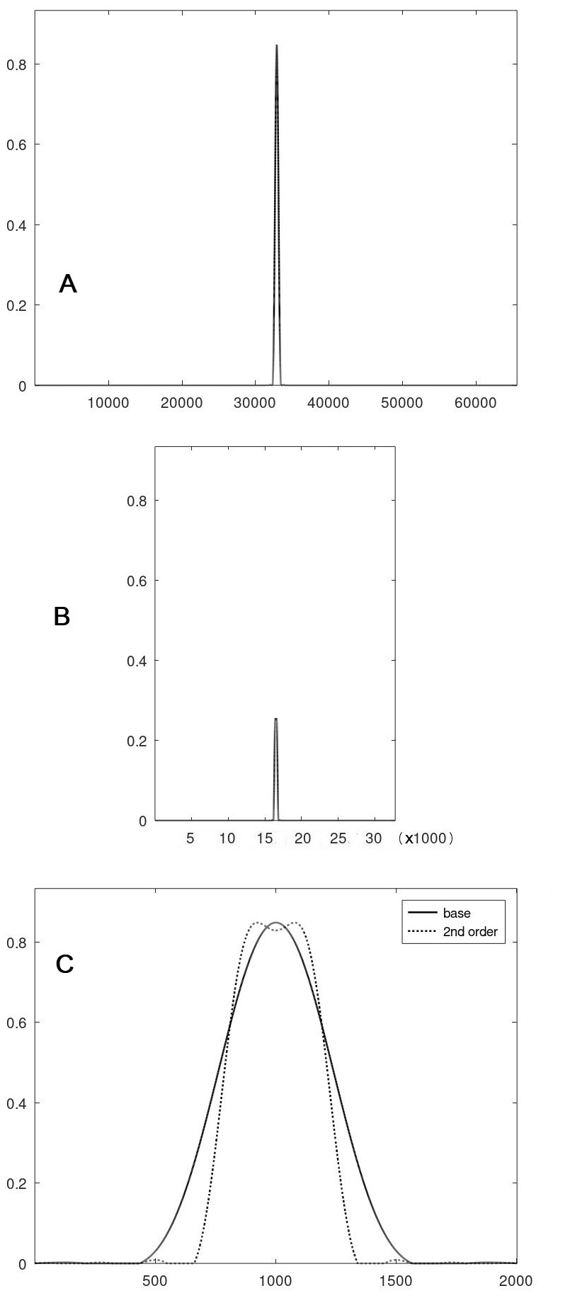
Figure 4: Case 3. Maps of two not-resolved point sources. A. Base. FT length=65536. B. 2nd-order. FT length=32768. C. The central parts of A (solid line) and B (dotted line). Length=2001.

The purpose of this study is to visually show the case in which two point sources are so closely located that they are not resolved in either the base or 2nd-order maps.

Two point sources have the same amplitude of 1.0 and are located at 0 unit and 1.0 unit, respectively. Three maps, as shown in Fig. 4, are generated in the same way as in Case 1. It can be seen in map C that the 2 peaks of the base map are completely merged to one peak (solid line). In contrast, the 2 peaks of the 2nd-order map are not completely merged (dotted line) , and the top center is convex downward, which is an indication that 2 distinct peaks might exist.

3.4 Case 4. Extended source

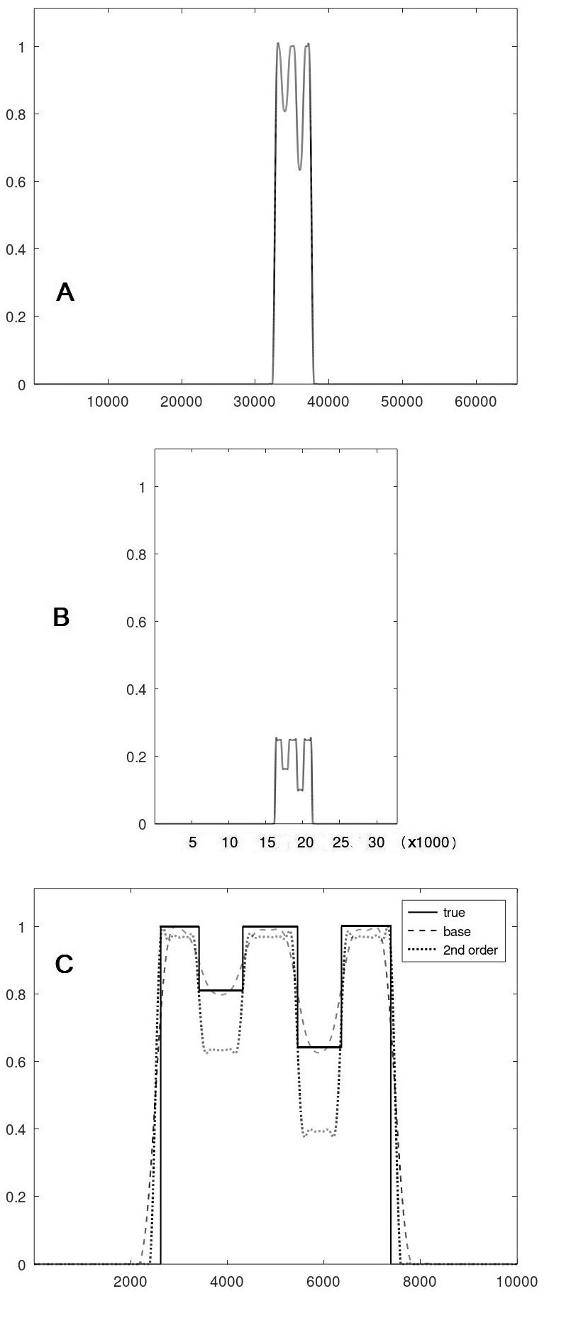
Figure 5: Case 4. Maps of an extended source. A. Base. FT length=65536. B. 2nd-order. FT length=32768. C. The central parts of the true image (solid line), A (dashed line) and B (dotted line). Length=10001.

The purpose of this study is to compare, with the “true image” as a reference, the images of an extended source in the base and 2nd-order maps. The extended source is a plateau having a flat top with 2 notches (see Fig. 5.C, solid line). The point-source model is used for the extended source, that is, it is represented with a number of points.

Three maps, as shown in Fig. 5, are generated in the same way as in Case 1. The central parts are shown in map C. Shown in this map additionally is the central part of the true image.

It can be seen in the 2nd-order map B that the image has sharp edges. In contrast, the image’s edges in the base map A are unclear. This difference can be seen more easily in map C with the true image as the reference.

4 Discussion

In this section we discuss some practical issues in the implementation of HOHI.

4.1 Generation of the second order harmonics

As shown in Fig. 1, the conventional correlator $\mathrm{C}_{1}$ and second order correlator $\mathrm{C}_{2}$ share the same preprocessed signals as their inputs. With the existing ASRT, for each baseline we need only to build $\mathrm{C}_{2}$ according to the formula $(a+ib)^{2}=(a^{2}-b^{2})+i2ab$. The visibility $V_{2,m}$ is generated according to Eq. 3.

4.2 Baselines and antenna array

Usually, the increment $d$ is chosen critically in designing an antenna array. The WSF determined by $\lambda/d$ and the FOV determined by antenna parameters have been carefully chosen in order to eliminate aliasing caused by strong radio sources inside the FOV but outside the WSF. The reduction of WSF may cause the aliasing problem.

In terms of signal processing, $d$ is the sampling interval. Doubling it may cause the problem of undersampling, and hence aliasing, depending on the lowpass filter effect of the antenna beam pattern.

In order to avoid this aliasing problem, the increment after being stretched must be kept as designed. Specifically, the increment of the real baseline must be $\frac{1}{2}d$ that will be stretched to $d$.

Let us look into the simplest east-west antenna array that consists of two antennas, one being fixed at the west end (antenna 0) while the other being movable, as shown schematically on the “Base” axis in Fig. 6. The movable antenna takes 4 positions, $1,2,3$ and $4$, which provides the 4 “real baselines” $\overline{0-1},\overline{0-2},\overline{0-3}$ and $\overline{0-4}$ with the increment $d$. The corresponding 4 “virtual baselines” are $\overline{0-2},\overline{0-4},\overline{0-6}$ and $\overline{0-8}$ with the increment $2d$, as shown on the “2nd” axis in Fig. 6. For the increment after being stretched to be $d$, the movable antenna takes $4$ more positions, $\mathrm{A}_{1},\mathrm{A}_{2},\mathrm{A}_{3}$ and $\mathrm{A}_{4}$, represented by the $4$ crosses at the midpoints of $\overline{0-1},\overline{1-2},\overline{2-3}$ and $\overline{3-4}$, respectively. As a result, 4 additional virtual baselines are generated. They are $\overline{0-1},\overline{0-3},\overline{0-5}$ and $\overline{0-7}$ on the 2nd axis. The whole set of 8 virtual baselines, $\overline{0-1},\overline{0-2},\dots,\overline{0-8}$, provides the desirable increment $d$.

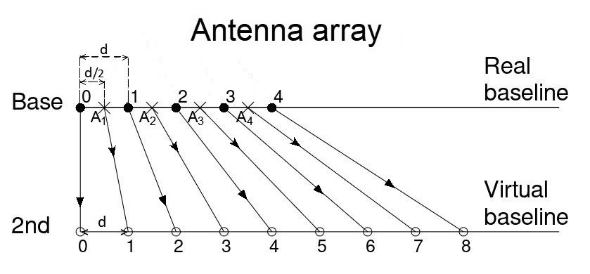
Figure 6: Antenna array and baselines. Base axis: Dots represent the existing antenna positions; crosses represent the added antenna positions.  2nd axis: Circles represent all the virtual positions of antennas.

For this simplest antenna array, doubling the number of baselines means doubling the number of positions the movable antenna takes, that is to say, the observation time will be doubled. This is the price we must pay for the improved resolvability as if the maximum baseline of array were doubled. For other antenna array configurations, this proportionality may not hold. The required number of positions the movable antennas take, and hence the observation time, may be increased by a factor of less than $2$ by utilizing “unused” baselines in the antenna spacings. On the other hand, in the general case, some required additional positions of the movable antennas may not be realizable because of physical constraints. As a consequence, some required virtual baselines may be missing.

4.3 Test at DRAO

The telescope of DRAO is suitable for the test of HOHI. Its linear array consists of $7$ east-west antennas, of which $2$ are fixed respectively at the $2$ ends of the array, and the other $5$ are movable along the rail. As a matter of fact, some basic parameters used in our computer simulation are taken from this antenna array, namely, $\lambda=0.21$ meter, $d=4.286$ meters, and $b_{M}=617.184$ meters.

Because of the constraint imposed by the terrain surrounding DRAO, it is very difficult, if not impossible, to extend the antenna array. Therefore, it makes sense to improve the resolvability of the telescope utilizing the technique of HOHI.

As declared in Landecker et al. [2019] concerning the renewal of the telescope of DRAO, it is an open testbed for Canadian innovation. We hope that our test will be carried out at DRAO and make a significant contribution to the development of radio astronomy.

5 Conclusions

Computer simulation has validated the theoretical analysis of the HOHI of second order. The resolvability of the telescope is improved by a factor of 2. Test may be carried out utilizing facilities at DRAO.

References

- Eaton et al. [2022] J. W. Eaton, D. Bateman, S. Hauberg, & R. Wehbring. GNU Octave version 7.3.0 manual: a high-level interactive language for numerical computations, 2022. URL https://www.gnu.org/software/octave/doc/v7.3.0/.
- Landecker et al. [2019] T. Landecker, L. Belostotski, J.-A. Brown, et al. DRAO Synthesis Telescope. e-prints [arXiv:1910.12002], Oct. 2019.
- Landecker et al. [2000] T. L. Landecker, P. E. Dewdney, T. A. Burgess, et al. The synthesis telescope at the dominion radio astrophysical observatory. A&AS, 145:509–524, 2000.
- Wu [1996] N. Wu. Proposed high order harmonic interferometer for aperture synthesis radio telescope. In G. H. Jacoby and J. Barnes, editors, Astronomical Data Analysis Software and Systems V, ASP Conf. Ser. 101, pages 215–218, San Francisco, 1996. Astronomical Society of the Pacific.