A Tutorial on the Pretrain-Finetune Paradigm for Natural Language Processing

Abstract

The pretrain-finetune paradigm represents a transformative approach in natural language processing (NLP). This paradigm distinguishes itself through the use of large pretrained language models, demonstrating remarkable efficiency in finetuning tasks, even with limited training data. This efficiency is especially beneficial for research in social sciences, where the number of annotated samples is often quite limited. Our tutorial offers a comprehensive introduction to the pretrain-finetune paradigm. We first delve into the fundamental concepts of pretraining and finetuning, followed by practical exercises using real-world applications. We demonstrate the application of the paradigm across various tasks, including multi-class classification and regression. Emphasizing its efficacy and user-friendliness, the tutorial aims to encourage broader adoption of this paradigm. To this end, we have provided open access to all our code and datasets. The tutorial is particularly valuable for quantitative researchers in psychology, offering them an insightful guide into this innovative approach.

Keywords: Large language models, pretrain-finetune, natural language processing

1 Introduction

The rise of pretrain-finetune paradigm has greatly reshaped the landscape of natural language processing (NLP) (E. Hu ., 2022). This new paradigm, characterized by the application of large pretrained language models, most notably BERT (Devlin ., 2019) and RoBERTa (Liu ., 2019), and high efficacy on finetuned tasks even in the face of relatively few training samples, is now being widely applied in social sciences (Zhang ., 2021; Wang, 20231, 20232). While earlier works have recommended a minimum of 3,000 samples for NLP tasks using the bag-of-words approach (Wang ., 2022), recent research applying the pretrain-finetune paradigm has shown that finetuned large models with just a few hundred labeled samples could yield competitive performance (Wang, 20232).

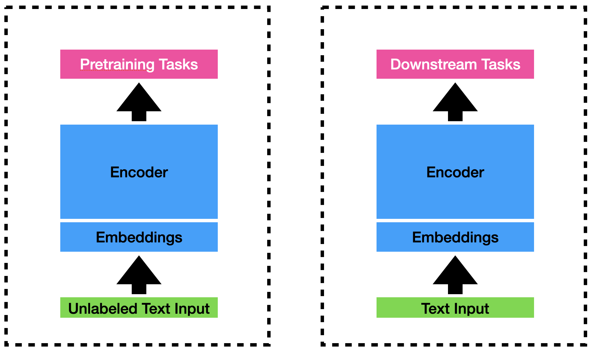
Figure 1: High-level illustration of the pretraining (left) and finetuning (right) workflows.

In the current tutorial, we aim to provide (1) an overview of the pretrain-finetune paradigm and (2) illustrative applications of the pretrain-finetune paradigm to research questions in social sciences (Figure 1). We first provide an introduction to the key concepts in pretraining and finetuning, such as tokenization and encoding. We then use some of the most recent applications of the pretrain-finetune paradigm in social sciences to illustrate how to use this paradigm to advance quantitative research in our discipline.

2 Pretrain

Pretraining is the process of training a model with unlabeled raw data with no particular downstream tasks. Some of the most widely used pretrained models include BERT and RoBERTa. These large language models usually contain hundreds of millions of parameters. Pretraining these models from scratch requires access to large amounts of raw data and specialized hardware like graphics processing units (GPUs). The pretraining process consists of the following steps: (1) tokenization, (2) encoding, and (3) pretraining tasks, such as masked language modeling, next sentence prediction (Devlin ., 2019) and sentence-order prediction (Lan ., 2020).

2.1 Tokenization

Unlike earlier methods such as bag of words (Wang ., 2022) or word embeddings (Mikolov ., 2013), large langauge models mostly use subwords as a token, such as wordpieces in BERT (Devlin ., 2019) and Byte-Pair Encoding (BPE) in RoBERTa (Liu ., 2019) and GPT-3 (Brown ., 2020). To illustrate how words are broken into subwords, let’s use a text snippet from the Journal’s description and tokenize it using the BPE tokenizer used in GPT-3.5 and GPT-4..

AMPPS encourages integration of methodological and analytical questions and
brings the latest methodological advances to non-methodology experts across
all areas of the field.

The word “AMPPS” is split into “AM”, “PP” and “S”. The word “methodological” is split into “method”, “ological”. And lastly the word “non-methodology” is split into “non”, “-method”, and “ology”. All other words, including punctuation marks, remain individual units without further splitting. These units are then turned into tokens represented with non-negative integers.

AM PP S encourages integration of method ological and analytical questions
and brings the latest method ological advances to non -method ology
experts across all areas of the field .

These units are then turned into tokens represented with integers.

[1428, 4505, 50, 37167, 18052, 315, 1749, 5848, 323, 44064, 4860, 323, 12716,
279, 5652, 1749, 5848, 31003, 311, 2536, 51397, 2508, 11909, 4028, 682, 5789,
315, 279, 2115, 627]

2.2 Encoding

Once we have tokenized the input text into tokens, we then retrieve the corresponding embeddings for these tokens, where the token id, a non-negative integer, would serve the retrieval key. These token embeddings are vector representations. For the BERT-large model, each such vector contains 1024 float numbers. These sets of vectors are then fed into the encoder layers.

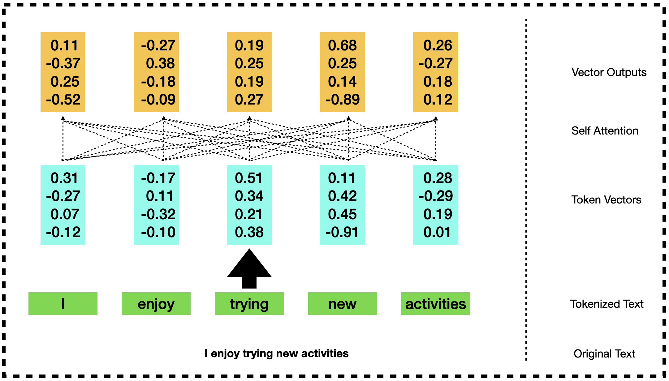
Figure 2: Illustration of the BERT model’s self-attention mechanism.

The key component of the encoders is self-attention (Vaswani ., 2017). Intuitively, it computes how much attention each token pays to the other tokens and generates the new representation for a token by calculating the weighted average of all the tokens where the weight is based on self-attention. Such encoders are then put on top of each other in a sequential manner. For example, in BERT-large models there are 24 encoder layers. In BERT-base models there are 12 encoder layers.

2.3 Pretraining tasks

Now that we have a good understanding of tokenization and encoding, let’s proceed to discuss how these parameters in these layers are trained using pretraining tasks. The goal is to train these large language models from scratch and embue them with world knowledge that exists in the training corpus (Longpre ., 2020). Commonly used pretraining tasks include masked language modeling, next sentence prediction (Devlin ., 2019) and sentence order prediction (Lan ., 2020).

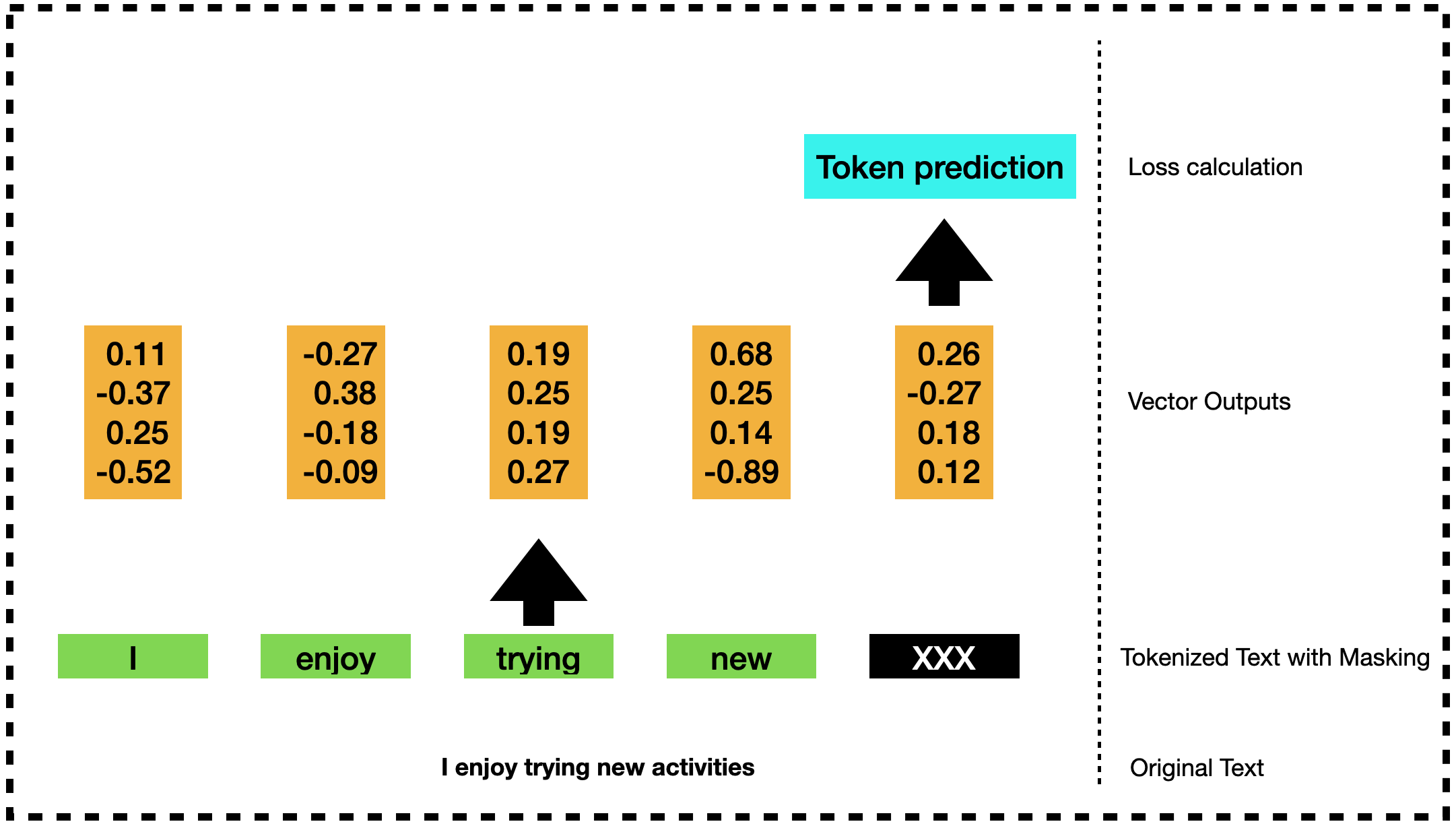
Figure 3: Illustration of the BERT model’s masked language modeling.

Let’s see an example of how masked language modeling works. Suppose we have the following input text: “I enjoy trying new activities”. During training, some of the tokens will be randomly masked and the language model is tasked with predicting these masked tokens. In Figure 3, the token “activities” is masked. The language model then is tasked with predicting this masked token. All tokens in the vocabulary are eligible candidates. Suppose the model predicts “activities” with a probability of 0.2. If we use cross entropy loss, then the loss term for this prediction is -log(0.2), which is its negative log-likelihood. Note that the higher probability the model assigns to the corrected token, the lower the loss. The language model is trained on this task over the entire corpus for a few times until the loss in prediction stops decreasing.

3 Finetuning

Finetuning is the process of training an already-pretrained model on a downstream task. It is characterized by (1) adding a small set new parameters to accommodate the new tasks and (2) a relatively small learning rate given the fact that the vast majority of the parameters are already reasonably trained during the pretraining stage. Downstream tasks at this stage can be broadly grouped into classification and regression. Examples of classification tasks include sentiment analysis and topic classification; examples of regression include fatality prediction. This is the step where quantitative psychologists need to apply a pretrained model to a particular task, such as depression detection and personality classification. For each specific task, researchers need to specify the model’s input, targeted output (including the number of labels), and whether this is a classification task or a regression task.

Figure 4: Illustration of the finetuning process. Same as with pretraining, the model takes in a text input and generates an encoding for each token. What differentiates finetuning from pretraining is that it takes a particular token representation to make task-specific predictions.

In Figure 4, we illustrate how a k-class classification works. From the encoder layers, we retrieve a 1 by N vector for each input sample, where N is 768 in the case of BERT-base and 1024 in the case of BERT-large. Then we project this vector to 1 by K using an N by K matrix. This layer is often referred to as the fully connected layer. What follows next depends on whether the task is classification or regression. In the case of classification, where K is equal to or greater than 2, we apply a softmax function such that each of the K elements represents the probability of that corresponding class being the predicted class:

$$softmax(x_{i})=\frac{exp(x_{i})}{\sum_{j}(exp(x_{j}))}$$

In the case of regression, where K is 1, we can apply the loss function directly to the 1 by K vector (now 1 by 1). Mean squared error is a commonly used loss function for regression tasks.

4 Practical Exercises

In this section, we provide two practical exercises to illustrate how researchers can finetune a large language model with relative ease to achieve state-of-the-art results in classification and regression, respectively. All our exercises are written in Python in the format of Jupyter notebooks so that readers can follow along in an interactive manner. For easy reproducibility and access to computation resources, all our computation is done on Google Colab.

4.1 Multi-class classification

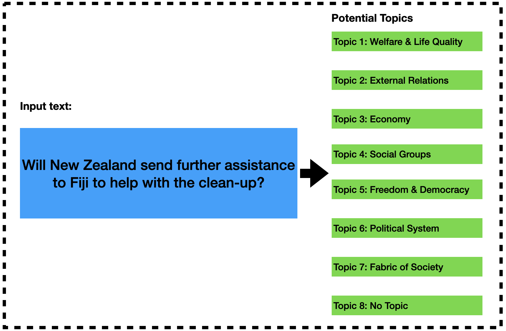
Figure 5: Given an input text, we categorize it into one of eight mutually exclusive classes. In the provided example, the text is classified under the second topic, External Relations.

When researchers need to classify text inputs into more than two classes, this is what we call multi-class classification. In the following case study, we classify a given text into one of eight topics. The texts are the speech transcripts from the New Zealand Parliament from 1987 to 2002 (Osnabrügge ., 2021). In Figure 5, we illustrate the data input and list all the eight classes. We use using 2,915 annotated speech transcripts for training, 625 for validation, and another 625 for testing.

We finetune a RoBERTa-base model (Liu ., 2019) for topic classification. RoBERTa-base has 12 layers of transformers and 125 million parameters in total. On top of its 12 layers of transformers, we add a classification layer for 8-topic classification. We use cross entropy as the loss function. We finetune the RoBERTa-base model for 20 epochs with a learning rate of 2e-5, a batch size of 16, and an input sequence length of 512 on an A100 GPU. We use the validation set’s cross entropy loss to select the best epoch and the optimal checkpoint. We then use the optimal checkpoint to make inferences on the test set with a batch size of 64 (see Listing 1). As our baseline, we use results from Osnabrügge . (2021), where the authors use 115,410 related but out-of-domain policy statements from Australia, Canada, Ireland, New Zealand, the United Kingdom, and the United States to train a regularized multinomial logistic regression model. For easy comparison, we use the same evaluation metrics as in Osnabrügge . (2021).

⬇

1

2 training_args = TrainingArguments(

3 output_dir="./results", # output directory

4 num_train_epochs=epochs, # total number of training epochs

5 per_device_train_batch_size=16, # batch size for training

6 per_device_eval_batch_size=64, # batch size for evaluation

7 learning_rate = 2e-5, # learning rate

8 save_strategy= "epoch", # save checkpoints after each epoch

9 evaluation_strategy="epoch",

10 load_best_model_at_end= True,

11 )

12

13 def model_init():

14 return RobertaForSequenceClassification.from_pretrained("roberta-base", num_labels=8) # number of labels

Listing 1: Specify the number of labels to be 8 for the multi-class classification and set the hyperparameters such as batch size and learning rate.

Across all metrics, finetuning the RoBERTa model with 2,915 New Zealand parliamentary speeches substantially outperforms the cross-domain topic classifier by Osnabrügge . (2021), which is trained using 115,420 annotated policy statements (Table 1). For example, for top-1 accuracy the finetuned RoBERTa model outperforms the cross-domain baseline by 26%. For top-3 accuracy the finetuned RoBERTa model outperforms the cross-domain baseline by 10%.

Table 1: Finetuning a RoBERTa-base model with 2,915 labeled in-domain samples can outperform the cross-domain regularized multinomial logistic regression model, trained with 115,420 out-of-domain samples, in the 8-topic classification task by a large margin. Cross-domain classifiers are from Osnabrügge . (2021). Test set is the same for both models. Mean of three random runs is reported, with standard deviation in the brackets. Better results are in bold.

Metrics	8 topics
	Cross-domain	Finetuning LM
Top-1 accuracy	0.512 (0.007)	0.643 (0.007)
Top-3 accuracy	0.821 (0.001)	0.899 (0.001)
Top-5 accuracy	0.917 (0.007)	0.968 (0.007)
Balanced accuracy	0.465 (0.004)	0.592 (0.004)
F1 macro	0.456 (0.011)	0.584 (0.011)

4.2 Regression

In regression tasks, researchers use an input text to predict a numerical value. In the following exercise, we predict the natural logarithm of fatalities on a country month level using the CrisisWatch text (Häffner ., 2023). For a visual representation of the input and output, please refer to Figure 6.

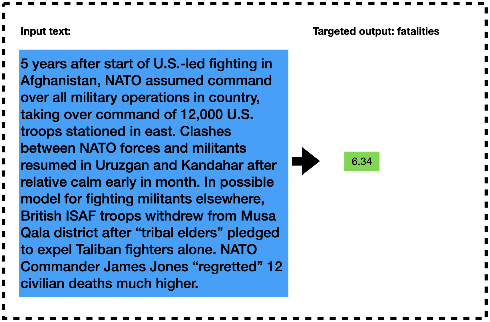
Figure 6: Given an input text, we predict a numerical value. In the example above, given an expert-written International Crisis Group (ICG) CrisisWatch report on Afghanistan for October, 2006, the model is expected to predict 6.34 as the natural logarithm of fatalities.

In Häffner . (2023), for the task of predicting the natural logarithm of fatalities on a country month level using the CrisisWatch text, the authors use random forest and XGBoost. The training set covers the period from 2003 to first half of 2020 and has 21,924 samples, the validation set covers the second half of 2020 and has 648 samples, and the test set covers the year 2021 and has 1296 samples. These two models achieve an R² of 0.64 and 0.63 respectively and an MSE of 1.59 and 1.60 respectively. We use the same training set, validation set and testing set as in Häffner . (2023). The large language model we use is ConfliBERT (Y. Hu ., 2022). ConfliBERT has the same architecture as BERT-base and is pretrained from scratch using a large corpus in the politics and conflicts domain. When we finetune ConfliBERT using CrisisWatch texts, we set the learning rate to 2e-5 and set the number of training epochs from 10 (see Listing 2).

⬇

1BASE_MODEL = "snowood1/ConfliBERT-scr-uncased" # pretrained model

2LEARNING_RATE = 2e-5

3MAX_LENGTH = 256

4BATCH_SIZE = 16

5EPOCHS = 10

6

7training_args = TrainingArguments(

8 learning_rate=LEARNING_RATE, # learning rate

9 per_device_train_batch_size=BATCH_SIZE, # training batch size

10 per_device_eval_batch_size=BATCH_SIZE, # test batch size

11 num_train_epochs=EPOCHS, # number of training epochs

12 seed=123

13)

14

15tokenizer = AutoTokenizer.from_pretrained(BASE_MODEL)

16

17def model_init():

18 model = AutoModelForSequenceClassification.from_pretrained(BASE_MODEL, num_labels=1, ignore_mismatched_sizes=True) # number of labels

19 return model

20

21def preprocess_function(examples):

22 label = examples["fatalities_log"]

23 examples = tokenizer(examples["final_text"], truncation=True, padding="max_length", max_length=256) # max sequence length

24 examples["label"] = float(label)

25 return examples

26

27class RegressionTrainer(Trainer):

28 def compute_loss(self, model, inputs, return_outputs=False):

29 labels = inputs.pop("labels")

30 outputs = model(**inputs)

31 logits = outputs[0][:, 0]

32 loss = torch.nn.functional.mse_loss(logits, labels)

33 return (loss, outputs) if return_outputs else loss

Listing 2: Specify the number of labels to be 1 for the regression task and set the hyperparameters such as batch size and learning rate.

We report two groups of finetuning results: ConfliBERT Length-256, where we set the max number of tokens to 256 and ConfliBERT Length-512, where we set the maximum sequence length to 512 (Wang, 20232). In Table 2, we compare the performance of finedtuned ConfliBERT models with that of two baseline models. OCoDi-Random Forest is the dictionary-based model that leverages random forest, where OCoDi stands for Objective Conflict Dictionary. OCoDi-XGBoost is the dictionary-based model that leverages XGBoost (Häffner ., 2023).

Table 2: Finetuned ConfliBERT models outperform dictionary-based models by a large margin. Results in Columns 1 and 2 are from Table 2 in Häffner . (2023). By increasing the maximum sequence length to 512, we are able to further improve the performance of those finetuned models. Best results in bold.

Model	OCoDi Random Forest (1)	OCoDi XGBoost (2)	ConfliBERT Length-256 (3)	ConfliBERT Length-512 (4)
MSE	1.59	1.60	0.99	0.82
R2	0.64	0.63	0.77	0.81

We observe that by finetuning ConfliBERT (Column 3), we are able to achieve a much lower mean squared error and a substantially higher R² than the dictionary-based approaches. Further, by increasing the maximum sequence length from 256 to 512 (Column 4), we observe that the mean squared error on the test set decreases from 0.99 to 0.82 and that the R² on the test set increases from 0.77 to 0.81. Comparing OCoDi-XGBoost and ConfliBERT Max Length, we observe that a finetuned ConfliBERT is able to achieve an MSE that is 49% lower than OCoDi-XGBoost and an R² that is 29% higher.

5 Conclusion

The pretrain-finetune paradigm has revolutionized the field of natural language processing. In this tutorial, we have provided an intuitive and thorough walk-through of the key concepts therein. We also introduced some of the most common use cases that the pretrain-finetune paradigm supports. To help facilitate the wider adoption of this new paradigm, we have included easy-to-follow examples and made the related datasets and scripts publicly available. Practitioners and scholars in quantitative psychology and psychology more broadly should find our tutorial useful.

References

- Brown \BOthers. (\APACyear2020) \APACinsertmetastargpt3{APACrefauthors}Brown, T., Mann, B., Ryder, N., Subbiah, M., Kaplan, J\BPBID., Dhariwal, P.\BDBLAmodei, D. \APACrefYearMonthDay2020. \BBOQ\APACrefatitleLanguage Models are Few-Shot Learners Language models are few-shot learners.\BBCQ \APACjournalVolNumPages34th Conference on Neural Information Processing Systems (NeurIPS 2020). \PrintBackRefs\CurrentBib
- Devlin \BOthers. (\APACyear2019) \APACinsertmetastarbert{APACrefauthors}Devlin, J., Chang, M\BHBIW., Lee, K.\BCBL \BBA Toutanova, K. \APACrefYearMonthDay2019. \BBOQ\APACrefatitleBERT: Pre-training of Deep Bidirectional Transformers for Language Understanding BERT: Pre-training of Deep Bidirectional Transformers for Language Understanding.\BBCQ \APACjournalVolNumPagesProceedings of NAACL-HLT4171-4186. \PrintBackRefs\CurrentBib
- E. Hu \BOthers. (\APACyear2022) \APACinsertmetastarlora{APACrefauthors}Hu, E., Shen, Y., Wallis, P., Allen-Zhu, Z., Li, Y., Wang, S.\BDBLChen, W. \APACrefYearMonthDay2022. \BBOQ\APACrefatitleLoRA: Low-Rank Adaptation of Large Language Models Lora: Low-rank adaptation of large language models.\BBCQ \APACjournalVolNumPagesProceedings of the International Conference on Learning Representations. \PrintBackRefs\CurrentBib
- Y. Hu \BOthers. (\APACyear2022) \APACinsertmetastarconflibert{APACrefauthors}Hu, Y., Hosseini, M., Parolin, E\BPBIS., Osorio, J., Khan, L., Brandt, P\BPBIT.\BCBL \BBA D’Orazio, V\BPBIJ. \APACrefYearMonthDay2022. \BBOQ\APACrefatitleConfliBERT: A Pre-trained Language Model for Political Conflict and Violence Conflibert: A pre-trained language model for political conflict and violence.\BBCQ \APACjournalVolNumPagesProceedings of the 2022 Conference of the North American Chapter of the Association for Computational Linguistics. \PrintBackRefs\CurrentBib
- Häffner \BOthers. (\APACyear2023) \APACinsertmetastarinterpretable{APACrefauthors}Häffner, S., Hofer, M., Nagl, M.\BCBL \BBA Walterskirchen, J. \APACrefYearMonthDay2023. \BBOQ\APACrefatitleIntroducing an Interpretable Deep Learning Approach to Domain-Specific Dictionary Creation: A Use Case for Conflict Prediction Introducing an interpretable deep learning approach to domain-specific dictionary creation: A use case for conflict prediction.\BBCQ \APACjournalVolNumPagesPolitical Analysis1–19. {APACrefDOI} \doi10.1017/pan.2023.7 \PrintBackRefs\CurrentBib
- Kjell \BOthers. (\APACyear2023) \APACinsertmetastartext_package{APACrefauthors}Kjell, O., Giorgi, S.\BCBL \BBA Schwartz, H\BPBIA. \APACrefYearMonthDay2023. \BBOQ\APACrefatitleThe Text-Package: An R-Package for Analyzing and Visualizing Human Language Using Normal Language Processing and Transformers The text-package: An r-package for analyzing and visualizing human language using normal language processing and transformers.\BBCQ \APACjournalVolNumPagesPsychological Methods. \PrintBackRefs\CurrentBib
- Lan \BOthers. (\APACyear2020) \APACinsertmetastaralbert{APACrefauthors}Lan, Z., Chen, M., Goodman, S., Gimpel, K., Sharma, P.\BCBL \BBA Soricut, R. \APACrefYearMonthDay2020. \BBOQ\APACrefatitleALBERT: A Lite BERT for Self-supervised Learning of Language Representations ALBERT: A Lite BERT for Self-supervised Learning of Language Representations.\BBCQ \APACjournalVolNumPagesICLR. \PrintBackRefs\CurrentBib
- Liu \BOthers. (\APACyear2019) \APACinsertmetastarroberta{APACrefauthors}Liu, Y., Ott, M., Goyal, N., Du, J., Joshi, M., Chen, D.\BDBLStoyanov, V. \APACrefYearMonthDay2019. \BBOQ\APACrefatitleRoBERTa: A Robustly Optimized BERT Pretraining Approach RoBERTa: A Robustly Optimized BERT Pretraining Approach.\BBCQ \APACjournalVolNumPagesarXiv:1907.11692. \PrintBackRefs\CurrentBib
- Longpre \BOthers. (\APACyear2020) \APACinsertmetastaraug{APACrefauthors}Longpre, S., Wang, Y.\BCBL \BBA DuBois, C. \APACrefYearMonthDay2020. \BBOQ\APACrefatitleHow Effective is Task-Agnostic Data Augmentation for Pretrained Transformers? How Effective is Task-Agnostic Data Augmentation for Pretrained Transformers?\BBCQ \APACjournalVolNumPagesFindings of the Association for Computational Linguistics: EMNLP 2020. \PrintBackRefs\CurrentBib
- Mikolov \BOthers. (\APACyear2013) \APACinsertmetastarword2vec{APACrefauthors}Mikolov, T., Sutskever, I., Chen, K., Corrado, G.\BCBL \BBA Dean, J. \APACrefYearMonthDay2013. \BBOQ\APACrefatitleDistributed Representations of Words and Phrases and their Compositionality Distributed representations of words and phrases and their compositionality.\BBCQ \APACjournalVolNumPagesNIPS’13: Proceedings of the 26th International Conference on Neural Information Processing Systems. \PrintBackRefs\CurrentBib
- Osnabrügge \BOthers. (\APACyear2021) \APACinsertmetastarcross_domain{APACrefauthors}Osnabrügge, M., Ash, E.\BCBL \BBA Morelli, M. \APACrefYearMonthDay2021. \BBOQ\APACrefatitleCross-Domain Topic Classification for Political Texts Cross-Domain Topic Classification for Political Texts.\BBCQ \APACjournalVolNumPagesPolitical Analysis. \PrintBackRefs\CurrentBib
- Pargent \BOthers. (\APACyear2023) \APACinsertmetastarbest_practices_supervised_ml{APACrefauthors}Pargent, F., Schoedel, R.\BCBL \BBA Stachl, C. \APACrefYearMonthDay2023. \BBOQ\APACrefatitleBest Practices in Supervised Machine Learning: A Tutorial for Psychologists Best practices in supervised machine learning: A tutorial for psychologists.\BBCQ \APACjournalVolNumPagesAdvances in Methods and Practices in Psychological Science. \PrintBackRefs\CurrentBib
- Vaswani \BOthers. (\APACyear2017) \APACinsertmetastarattention{APACrefauthors}Vaswani, A., Shazeer, N., Parmar, N., Uszkoreit, J., Jones, L., Gomez, A\BPBIN.\BDBLPolosukhin, I. \APACrefYearMonthDay2017. \BBOQ\APACrefatitleAttention Is All You Need Attention Is All You Need.\BBCQ \APACjournalVolNumPages31st Conference on Neural Information Processing Systems. \PrintBackRefs\CurrentBib
- Wang (\APACyear2019) \APACinsertmetastarpredicted_acc2{APACrefauthors}Wang, Y. \APACrefYearMonthDay2019. \BBOQ\APACrefatitleComparing Random Forest with Logistic Regression for Predicting Class-Imbalanced Civil War Onset Data: A Comment Comparing Random Forest with Logistic Regression for Predicting Class-Imbalanced Civil War Onset Data: A Comment.\BBCQ \APACjournalVolNumPagesPolitical Analysis211107-110. \PrintBackRefs\CurrentBib
- Wang (\APACyear2023\APACexlab\BCnt1) \APACinsertmetastarfinetune_pa{APACrefauthors}Wang, Y. \APACrefYearMonthDay2023\BCnt1. \BBOQ\APACrefatitleOn Finetuning Large Language Models On finetuning large language models.\BBCQ \APACjournalVolNumPagesPolitical Analysis. \PrintBackRefs\CurrentBib
- Wang (\APACyear2023\APACexlab\BCnt2) \APACinsertmetastarpretrained_topic_classification{APACrefauthors}Wang, Y. \APACrefYearMonthDay2023\BCnt2. \BBOQ\APACrefatitleTopic Classification for Political Texts with Pretrained Language Models Topic Classification for Political Texts with Pretrained Language Models.\BBCQ \APACjournalVolNumPagesPolitical Analysis. \PrintBackRefs\CurrentBib
- Wang \BOthers. (\APACyear2022) \APACinsertmetastarbag_of_words{APACrefauthors}Wang, Y., Tian, J., Yazar, Y., Ones, D\BPBIS.\BCBL \BBA Landers, R\BPBIN. \APACrefYearMonthDay2022. \BBOQ\APACrefatitleUsing Natural Language Processing and Machine Learning to Replace Human Content Coders Using natural language processing and machine learning to replace human content coders.\BBCQ \APACjournalVolNumPagesPsychological Methods. \PrintBackRefs\CurrentBib
- Zhang \BOthers. (\APACyear2021) \APACinsertmetastarmonitor_depression{APACrefauthors}Zhang, Y., Lyu, H., Liu, Y., Zhang, X., Wang, Y.\BCBL \BBA Luo, J. \APACrefYearMonthDay2021. \BBOQ\APACrefatitleMonitoring Depression Trends on Twitter During the COVID-19 Pandemic: Observational Study Monitoring depression trends on twitter during the covid-19 pandemic: Observational study.\BBCQ \APACjournalVolNumPagesJMIR Infodemiology. \PrintBackRefs\CurrentBib