eric: [1]˝: #1ForestGreen dc: [1]˝: #1blue Fig:

Characterizing Dynamic Majorana Hybridization
for Universal Quantum Computing

Abstract

Qubits built out of Majorana zero modes have long been theorized as a potential pathway toward fault-tolerant topological quantum computation. Almost unavoidable in these processes is Majorana wavefunction overlap, known as hybridization, which arise throughout the process when Majorana modes get close to each other. This breaks the ground state degeneracy, leading to qubit errors in the braiding process. This work presents an accessible method to track transitions within the low-energy subspace and predict the output of braids with hybridized Majorana modes. As an application, we characterize Pauli qubit-errors, as demonstrated on an X-gate, critical for the successful operation of any quantum computer. Further, we perform numerical simulations to demonstrate how to utilize the hybridization to implement arbitrary rotations, along with a two-qubit controlled magic gate, thus providing a demonstration of universal quantum computing.

Introduction.— Topological quantum computing presents one of the most exciting avenues towards fault-tolerant quantum computation Kitaev (2003); Nayak et al. (2008). In essence, this depends on the storing and manipulation of quantum information non-locally in the form of Majorana zero modes (MZMs), zero energy subgap states that form on the boundaries of topological superconductors Kitaev (2001); Read and Green (2000). Promising platforms to host these exotic states range from semiconductor nanostructures Lutchyn et al. (2010); Oreg et al. (2010); Deng et al. (2016); Mourik et al. (2012); M. Aghaee et al. (2023) to magnet-superconductor hybrid systems Nadj-Perge et al. (2013); Ruby et al. (2015); Pawlak et al. (2016); Palacio-Morales et al. (2019); Schneider et al. (2021). MZMs obey non-Abelian statistics under exchange, otherwise known as a braid. Such an operation changes their quantum state, allowing for the encoding of unitary gates Bravyi and Kitaev (2002). Unlike most quantum computing platforms, non-locality protects the topological quantum bits and gates from the effects of local perturbation, providing an exciting avenue towards fault-tolerant quantum computing Nayak et al. (2008); Wang (2010); Sarma et al. (2015); Lahtinen and Pachos (2017).

While true MZMs remain at zero energy, in any finite, realistic system Majorana wavefunction overlap, known as hybridization, will perturb these states to finite energies Cheng et al. (2009). With the advent of superconducting nano-structures protected by small bulk energy gaps Li et al. (2014, 2016); Pahomi et al. (2020); Crawford et al. (2022); Li and Liu (2023) avoiding the overlap of MZMs in experiment becomes almost unavoidable. Previous works have reported oscillations in the fidelity of a braid Cheng et al. (2011); Amorim et al. (2015); Bauer et al. (2018); Harper et al. (2019); Chen et al. (2022); Bedow et al. , however, a precise dynamical understanding of why this occurs remains unknown. Further, while topological protection is founded on the basis that the MZMs are well separated during braiding processes, braiding alone does not provide the basis for universal quantum computing Bravyi and Kitaev (2002). For use in universal quantum computing, we require some controlled hybridization protocol to implement the $\pi/4$-phase gate or T-gate Bonderson et al. (2010); Karzig et al. (2016, 2019), the missing piece for universal quantum computation based on MZMs. Thus, a complete understanding of how hybridization changes the many-body ground state is pivotal: (i) To well-define the way quantum operations are dynamically affected by the changing Majorana overlap throughout a braiding process. This would allow one to accurately quantify and correct for Pauli-qubit errors in a time-dependent process. (ii) To accurately predict the timescales required for the implementation of quantum gates based purely on time-dependent hybridization.

In this Letter, we utilise methods analogous to those used in Landau-Zener tunneling Garraway and Vitanov (1997); Nikitin (2006); Ivakhnenko et al. (2023) to make predictions for the effects of hybridization in dynamical braiding processes. Such methods have been utilised previously for a pair of vortices in a $p$-wave superconductor with fixed distance, corresponding to a pair of MZMs with fixed energy splitting Cheng et al. (2011) and to investigate non-adiabatic transitions to bulk states in Majorana exchange processes Scheurer and Shnirman (2013). Here we characterize the error for systems with multiple pairs of MZMs and time-dependent energy splitting. We also predict and simulate the T-gate or magic gate, along with an arbitrary phase gate along the $y$-axis, demonstrating how dynamic hybridization may be utilised to map an arbitrary state about the Bloch sphere. Finally, we extend the scope of our method to implement an arbitrary controlled-phase gate purely through hybridization.

Method.— We consider a time-dependent Hamiltonian $\mathcal{H}(t)$ of the form

$$\mathcal{H}(t)=\frac{1}{2}\Psi^{\dagger}\begin{pmatrix}h(t)&\Delta(t)\\[10.0pt] \Delta^{{\dagger}}(t)&-h^{T}(t)\end{pmatrix}\Psi~{}=\frac{1}{2}\Psi^{\dagger}H_{\textrm{BdG}}(t)\Psi$$ (1)

where $\Psi=(c_{1},...,c_{N},c^{{\dagger}}_{1},...,c^{{\dagger}}_{N})$. The $c_{n}$ ($c^{{\dagger}}_{n}$) are the annihilation (creation) operators for a bare electron with index $n$. We keep this general, as it may label multiple physical parameters such as the site, spin and orbital of the electron. $h_{nm}(t)$ is a time-dependent hopping between states $n$ and $m$, and $\Delta_{nm}(t)$ is the mean field pairing potential between such states. The time-dependent matrix $H_{\textrm{BdG}}(t)$ is known as the Bogoliubov–de Gennes (BdG) Hamiltonian. We may transform between superconducting quasiparticle operators $\{d_{i}\}$ and electron operators $\{c_{i}\}$ via a unitary Boguliubov transformation, given by $\hat{d}^{{\dagger}}_{i}=\hat{c}^{{\dagger}}_{j}U_{ji}+\hat{c}_{j}V_{ji}$ for some $U_{ij},V_{ij}\in\mathbb{C}$. This is such that $\mathcal{H}(0)=\sum_{i}E_{i}\hat{d}^{{\dagger}}_{i}\hat{d}_{i}-\frac{1}{2}\sum_{i}E_{i}$, with $E_{i}\geq 0$ the eigenenergies of the system.

To track the time-evolution of the state-space, we to need consider the time-evolution of the superconducting quasiparticles $\hat{d}_{i}(t)=\mathcal{S}(t,t_{0})\hat{d}_{i}(t_{0})\mathcal{S}^{{\dagger}}(t,t_{0})$, where $\mathcal{S}(t,t_{0})$ is the time-evolution operator. It is defined as $\mathcal{S}(t,t_{0})=\mathcal{T}\textrm{exp}(-i\int^{t}_{t_{0}}\mathcal{H}(t^{\prime})dt^{\prime})$, with $\mathcal{T}$ time-ordering the matrix exponential. The $\hat{d}^{{\dagger}}_{i}(t)$ create the dynamical single-particle state $|\Psi_{i}(t)\rangle$ by acting on the time-evolved quasiparticle vacuum, i.e., $\hat{d}^{{\dagger}}_{i}(t)|0(t)\rangle_{d}=|\Psi_{i}(t)\rangle$. By the time-dependent Boguliubov equations (TDBdG) Kümmel (1969); Cheng et al. (2011); Sanno et al. (2021) , $\hat{d}^{{\dagger}}_{i}(t)=\hat{c}^{{\dagger}}_{j}U_{ji}(t)+\hat{c}_{j}V_{ji}(t)$ remains connected to the bare electron basis by a Boguliubov transformation, where

$$\begin{pmatrix}U(t)\\ V(t)\end{pmatrix}=\mathcal{T}\textrm{exp}\left(-i\int^{t}_{0}H_{\textrm{BdG}}(t^{\prime})dt^{\prime}\right)\begin{pmatrix}U\\ V\end{pmatrix}.$$ (2)

Let $\{\Psi_{i}(t)\}$ be the dynamic wavefunctions, defined as $(\Psi_{1}(t),\Psi_{2}(t),...,\Psi_{N}(t))=(U(t),V(t))^{T}$. As $\Psi_{i}(t)$ is a Boguliubov wavefunction, we may represent it as an expansion of the set of instantaneous eigenvectors of $H_{\textrm{BdG}}(t)$, which are $\{\psi_{i}(t)\}$, as $\Psi_{i}(t)=\sum_{j}c^{i}_{j}(t)\psi_{j}(t)$. The $c^{i}_{j}(t)\in\mathbb{C}$ are coefficients that determine the time-dependent expansion in the instantaneous eigenstate basis, with initial condition $c^{i}_{j}(0)=\delta_{ij}$, which initialises $\Psi_{i}(0)=\psi_{i}(0)$. Using the TDBdG equation , we may track the evolution of the $c^{i}_{j}(t)$ coefficients via the following equation of motion:

$$\begin{split}\dot{c}^{i}_{j}(t)=-i\left(E(t)-A(t)\right)_{jk}c^{i}_{k}(t)=-iM_{jk}(t)c^{i}_{k}(t).\end{split}$$ (3)

Here, $E_{ij}(t)=\psi_{i}^{{\dagger}}(t)H_{\textrm{BdG}}(t)\psi_{j}(t)$. $A_{ij}(t)=i\psi^{{\dagger}}_{i}(t)\dot{\psi}_{j}(t)$ is the non-Abelian Berry matrix,Simon (1983); Berry (1984); Wilczek and Zee (1984), which acts as an instantaneous tunneling term between states. Solving this equation, we find that the adiabatic expansion coefficients $c^{i}_{j}(t)$ evolve as

$$c^{i}_{j}(t)=\mathcal{T}\textrm{exp}(-i\int^{t}_{t_{0}}M(t^{\prime})dt^{\prime})_{jk}c^{i}_{k}(t_{0}).$$ (4)

We set $I(t,t_{0})=\mathcal{T}\textrm{exp}(-i\int^{t}_{t_{0}}M(t^{\prime})dt^{\prime})$. In the context of dynamical braiding, Cheng, Galitski and Das Sarma derived this equation for a time-independent $M(t)=M$ in their pioneering work Cheng et al. (2011). Later, Scheurer and Shnirman considered varying $M(t)$, however, focussed on non-adiabatic interactions with low-lying bulk states Scheurer and Shnirman (2013). We expand this analysis to look at hybridization dynamics in systems with two, four and six MZMs.

For the purpose of tracking braiding outcomes, we will restrict our focus onto the ground-state manifold spanned by low energy subgap states made up of Majorana operators, defined by $\hat{d}^{{\dagger}}_{i}(t)=\frac{1}{\sqrt{2}}\big{(}\hat{\gamma}_{2i-1}(t)-i\hat{\gamma}_{2i}(t)\big{)}$. The MZM operators, $\{\hat{\gamma}_{i}\}$, are self-adjoint which obey fractional statistics under exchange, where if $\hat{\gamma}_{i}\to\hat{\gamma_{j}}$, then $\hat{\gamma}_{j}$ will transform as $\gamma_{j}\to-\hat{\gamma}_{i}$. Further, they follow fermionic anticommutation rules $\{\hat{\gamma}_{i},\hat{\gamma_{j}}\}=\delta_{ij}$. We map the time instantaneous wavefunctions $\{\psi_{i}(t)\}$ to the instantaneous MZM wavefunctions, $\{\psi^{\gamma}_{i}(t)\}$, by a change of basis matrix $S(t)$, such that $\Psi_{i}(t)=c^{i}_{k}(t)S_{km}(t)\psi^{\gamma}_{m}(t)$. We set $t_{0}=0$. With respect to a new expansion set of coefficients, $V_{ij}(t)$, we may expand the dynamic Majorana wavefunction $\Psi^{\gamma}_{i}(t)$ as $\Psi^{\gamma}_{i}(t)=V_{ik}(t)\psi^{\gamma}_{k}(0)$, with

$$V(t)=\left(S^{*}(t)I(t,0)S^{T}(0)\right)^{T}B^{T}(t,0).$$ (5)

Here, $B_{ij}(t)=\langle\psi_{i}^{\gamma}(0)|\psi^{\gamma}_{j}(t)\rangle$ is a connection term between the $\{|\psi^{\gamma}_{i}(0)\rangle\}$ and $\{|\psi^{\gamma}_{i}(t)\rangle\}$ state vectors. This will allow tracking of the state evolution, under any such dynamical braiding process, without the need for a full many-body simulation, assuming the MZM states only interact with other MZM states in the low energy subspace. Qubit information will be obtained by analysing time-dependent Pauli projections $\langle\hat{\sigma}_{i}(t)\rangle$, where the Majorana representation of these operators is given by $(\hat{\sigma}_{x},\hat{\sigma}_{y},\hat{\sigma}_{z})=2i(\hat{\gamma}_{3}\hat{\gamma}_{2},\hat{\gamma}_{1}\hat{\gamma}_{3},\hat{\gamma}_{2}\hat{\gamma}_{1})$. For more details see Supplementary Material (SM).

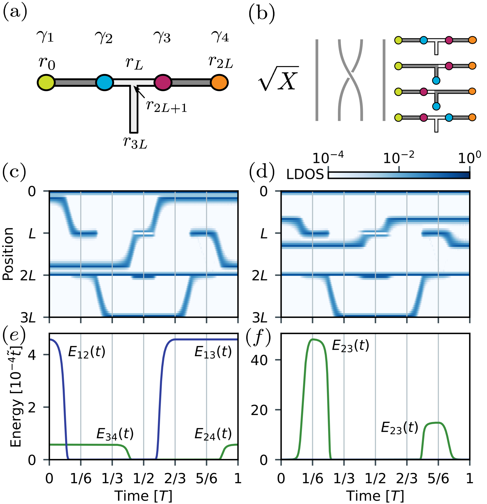
Figure 1: (a) Setup of T-junction with two pairs of MZMs separated by a trivial region. (b) $\sqrt{\textrm{X}}$ gate braiding protocol on a T-junction. (c) LDOS of MZM wavefunctions in the energy-splitting regime and (d) in the tunneling regime, respectively. (e) Instantaneous energies of the MZM energy couplings in the energy-splitting regime and (f) in the tunneling regime, respectively.

Results.— We consider a trijunction of Kitaev’s quantum wire model Kitaev (2001); Alicea et al. (2011), with each leg given by Eq. (1) with $h_{ij}=-\mu_{i}(t)\delta_{ij}-\tilde{t}(\delta_{i,j+1}+\delta_{i+1,j})$ and $\Delta_{ij}=e^{i\phi_{p}}|\Delta_{p}|(\delta_{ij+1}-\delta_{j+1,i})$. A graphic of this model is given in Fig. 1 a. We will set $|\tilde{t}|=|\Delta_{p}|=1$, with $\phi_{p}$=$0$, $\pi$, $\frac{\pi}{2}$ along the left, right and bottom leg respectively. While all simulations are conducted with these parameters, we are not restricted to this choice for the success of the method. The topological regime is defined by $\mu=\mu_{\textrm{topo}}$ for $-2<\mu_{\textrm{topo}}<2$, with MZMs emergent on the boundaries of the topological region. Consequently, $|\mu_{\textrm{triv}}|>2$ will define the trivial regime, with gap closings at $|\mu_{\textrm{triv}}|=2$. For a single qubit, information is stored in the two-level state $|\psi\rangle=\textrm{cos}(\frac{\theta}{2})|0\rangle_{\textrm{log}}+e^{i\phi}\textrm{sin}(\frac{\theta}{2})|1\rangle_{\textrm{log}}$, where $\theta\in[0,\pi]$, $\phi\in[0,2\pi]$. For $|0\rangle_{d}$ the unfilled ground state, satisfying $\hat{d}_{i}|0\rangle_{d}=0$, we define $|\bm{n}_{d}\rangle_{\textrm{phys}}=\prod_{k}(d^{{\dagger}}_{k})^{n_{k}}|0\rangle_{d}$, where $n_{k}$ is the occupancy of the $k$th state. For a single qubit system, we translate from the physical to the logical basis (even parity) by $|0\rangle_{\textrm{log}}=|00\rangle_{\textrm{phys}}$, $|1\rangle_{\textrm{log}}=\hat{d}_{1}^{{\dagger}}\hat{d}_{2}^{{\dagger}}|0\rangle_{d}=|11\rangle_{\textrm{phys}}$.

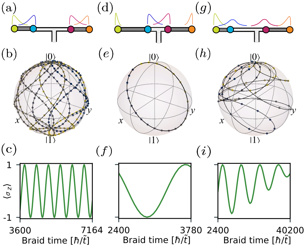
Figure 2: X-gate oscillations due to energy-splitting (first column), tunneling (second column) and combined-case regimes (third column). (a, d, g) Illustration of wavefunction overlaps. (b, e, h) Plotted on a Bloch-sphere, the final state outcomes, $|\Psi(T)\rangle$, as a function of total braid time for the X Gate, with analytical final state trajectories (solid line) plotted against many-body simulations (dots). (c, f, i) Pauli-Z projection, $\langle\hat{\sigma}_{z}(T)\rangle$, as a function of braiding time $T$. The parameter set for each case ($\mu_{\textrm{topo}}$, $\mu_{\textrm{triv}}$, $r_{12}$, $r_{34}$, $L$)=$(0.8,10,4a_{0},12a_{0},24a_{0})$, $(0.0,5.4,4a_{0},12a_{0},15a_{0})$, $(0.35,4.5,4a_{0},12a_{0},20a_{0})$ and initial state $|\psi\rangle=|0\rangle_{\rm log}$.

X-Gate Oscillations.— We begin by analysing the effects of Majorana hybridization on the Pauli $X$ gate outcome on a T-junction (for the analogous analysis for $\sqrt{\textrm{Z}}$-gate we refer the reader to the SM). The braiding routine required to perform this is illustrated in Fig. 1 b Alicea et al. (2011), with the Majorana modes moved by dynamic control of the chemical potential $\mu_{i}(t)$ on each site $i$. We simulate the braid for different total braid times $T$ Mascot et al. (2023) to investigate the effects of hybridization on the outcome of the final state. The low energy Hamiltonian may be written as $\mathcal{H}_{\textrm{eff}}(t)=\frac{i}{2}\sum_{ij}E_{ij}(t)\hat{\gamma}_{i}(t)\hat{\gamma}_{j}(t)$ Bauer et al. (2018). The energy coupling $E_{ij}(t)$ behaves as $E_{ij}(t)\sim e^{-r_{ij}(t)/\zeta(t)}$, where $r_{ij}$ the spatial separation between $\gamma_{i}$ and $\gamma_{j}$ and $\zeta$ the decay length of the Majorana wavefunctionCheng et al. (2009). This implies an energy coupling between $\gamma_{i}$ and $\gamma_{j}$ that scales with the wavefunction overlap of each Majorana fermion. The particle hole wavefunctions associated with each energy splitting $E_{ij}(t)$ is given by $\psi^{p/h}_{ij}(t)=\psi^{\gamma}_{i}(t)\mp i\psi^{\gamma}_{j}(t)$, where $p$ $(h)$ labels the particle (hole) state and $\psi^{\gamma}_{i}(t)$ is the wavefunction of $\gamma_{i}$. We expand the dynamic wavefunction $\Psi_{i}(t)$ in the subspace spanned by the $\{\psi^{p}_{12}(t),\psi^{h}_{12}(t),\psi^{p}_{34}(t),\psi^{h}_{34}(t)\}$ wavefunctions. We may write the coupling matrix $M(t)$ in the following block matrix form

$$M(t)=\begin{pmatrix}M_{12}(t)&M_{23}(t)\\ M^{T}_{23}(t)&M_{34}(t)\end{pmatrix}=M^{(1)}(t)+M^{(2)}(t),$$ (6)

where $M_{12}(t)=E_{12}(t)\sigma_{z}$ $+A_{12}(t)\sigma_{x}$ and $M_{23}(t)=-(\frac{E_{23}(t)}{2}+A_{13}(t))(\sigma_{z}+i\sigma_{y})$. Further, $M_{34}(t)$ has the same form as $M_{12}(t)$ up to index labelling, see SM. $M^{(1)}(t)$ corresponds to the block diagonal terms of $M(t)$ that drive transitions between the particle-hole states of same $\gamma_{i}$. Whereas, $M^{(2)}(t)$ are the off-diagonal contributions that lead to a tunneling between $|\psi^{p/h}_{12}(t)\rangle$ and $|\psi^{p/h}_{34}(t)\rangle$. The case where $M^{(2)}(t)$ terms are suppressed, we will denote as the energy-splitting regime. The case where $M^{(1)}(t)$ are diminished we will denote as the tunneling regime.

Initializing the state $|\psi\rangle=|0\rangle_{\textrm{log}}$, we simulate the braid for different total braid times $T$. We begin by analysing a regime where the dominant Majorana-coupling occurs through the topological region of the system, the energy-splitting regime. The overlap between the Majorana wavefunctions can be seen in the local density of states (LDOS), Fig. 1 c. This corresponds to the wavefunction density, as a function of time, of states in the low-energy subspace. Initially, the Majorana wavefunction overlap is between $\psi^{\gamma}_{1}$ $(\psi^{\gamma}_{3})$ and $\psi^{\gamma}_{2}$ $(\psi^{\gamma}_{4})$, as depicted in Fig. 2 a. This induces an energy splitting $E_{12}(t)$ ($E_{34}(t)$), as seen in Fig. 1 e. However, after the swap across the junction at $r_{L}$, $\psi^{\gamma}_{1}$ $(\psi^{\gamma}_{2})$ now overlaps with $\psi^{\gamma}_{3}$ $(\psi^{\gamma}_{4})$, leading to $E_{13}(t)$ and $E_{24}(t)$ contributions.

For a process approaching the adiabatic limit, Berry-matrix transitions, $A_{12}(t)$, $A_{34}(t)\sim v(t)e^{-r_{ij}/\zeta(t)}$, where $v(t)$ is a time-dependent function that scales with the speed of the process, and gets suppressed as $v(t)\to 0$ Cheng et al. (2011); Scheurer and Shnirman (2013). Furthermore, as $M^{(2)}(t)$ contributions are suppressed, we may solve analytically for the expectation values of the Pauli operators, $\langle\hat{\sigma}_{i}(T)\rangle$, as a function of braid time $T$ (even parity sector):

$$\langle\hat{\sigma}_{x}(T)\rangle=-\textrm{cos}\left(\bar{E_{2}}T\right)\textrm{sin}\left((\bar{E}_{1}+\bar{E_{2}})T\right)\ ,$$ (7)

$$\langle\hat{\sigma}_{y}(T)\rangle=\textrm{sin}\left(\bar{E_{2}}T\right)\textrm{sin}\left((\bar{E}_{1}+\bar{E_{2}})T\right)\ ,$$ (8)

$$\langle\hat{\sigma}_{z}(T)\rangle=-\textrm{cos}\left((\bar{E}_{1}+\bar{E}_{2})T\right)\ .$$ (9)

Results for the odd parity sector are similar (see SM). We note that a successful X braid would correspond to $\langle\hat{\sigma}_{z}(T)\rangle=-1$. Here, we have defined $\bar{E}_{ij}=\frac{1}{T}\int^{T}_{0}E_{ij}(t^{\prime})dt^{\prime}$ to be the average coupling energy between $\gamma_{i}$ and $\gamma_{j}$ throughout the process. Further, we define $\bar{E}_{1}=\bar{E}_{12}+\bar{E}_{34}$ and $\bar{E}_{2}=\bar{E}_{13}+\bar{E}_{24}$.

These results are compared to many-body simulations in Fig. 2 b and c. Notably, the $\langle\hat{\sigma}_{z}(T)\rangle$ projection, an equivalent measure of the transition probability $|\langle 1|0(T)\rangle_{\rm log}|^{2}$, oscillates as a function of total braid time, with period of oscillation $\tau=2\pi/(\bar{E}_{1}+\bar{E}_{2})$. This yields a striking result, as it allows for the prediction of the final state, without the need for a full simulation.

This process may similarly be conducted when the dominant overlap occurs through the trivial region of the T-junction, which we will refer to as the tunneling regime. As depicted in Fig. 2 b, we initialise the system with dominant Majorana wavefunction overlap between $\gamma_{2}$ and $\gamma_{3}$ which will remain throughout the process. As shown in Fig. 1 d and f, when Majorana separation $r_{23}$ reaches a minimal point crossing the junction, the induced $E_{23}(t)$ energy splitting reaches a maximum, tailing away as $\gamma_{2}$ leaves the junction. In this case, the final state projections are given by

$$\langle\hat{\sigma}_{x}(t)\rangle=0\ ,$$ (10)

$$\langle\hat{\sigma}_{y}(t)\rangle=-\textrm{sin}(2\bar{E}_{23}T+4\beta)\ ,$$ (11)

$$\langle\hat{\sigma}_{z}(t)\rangle=-\textrm{cos}(2\bar{E}_{23}T+4\beta)$$ (12)

where $\beta(T)=\int^{T}_{0}A_{23}(t^{\prime})dt^{\prime}$ is a path dependent quantity, and is independent of $T$. Unlike the energy-splitting case, the final state is restricted to the $yz$-plane of the Bloch-sphere, as shown in Fig. 2 e, with period of oscillation $\tau=\pi/\bar{E}_{23}$ a function of the average hybridization energy between $\gamma_{2}$ and $\gamma_{3}$ over the process. Crucially, both results may be used to probe the feasibility and time-scales required for a successful braiding result to occur on an arbitrary platform. The period of oscillation scales with the average hybridization energy arising from the Majorana couplings $\bar{E}_{ij}$. This allows for accurate prediction of the scale of qubit error in a process, pivotal not just for numerical simulation, but also for experimental implementation of a braiding process.

Finally, we consider the case where both energy-splitting and tunneling contribute to $M(t)$. As shown in Fig. 2 g, we initialise the system with dominant $\gamma_{1}$-$\gamma_{2}$ wavefunction overlap, inducing an $E_{12}(t)$ coupling. However as $\gamma_{2}$ approaches the junction, the key hybridization contribution becomes $E_{23}(t)$ as $\gamma_{2}-\gamma_{3}$ overlap starts to dominate, leading to a transition between the energy-splitting and tunneling regimes. Much like the energy splitting case, Fig. 2 h resembles a web-like structure in phase around the Bloch sphere. However, as can be seen in Fig. 2 i, the $\langle\hat{\sigma}_{z}(T)\rangle$ projection fails to reach $-1$ at the minimum, constituting a failed braid at all braid times $T$ measured. This constitutes the most difficult scenario to compute a successful braid, with $\langle\hat{\sigma}_{z}(T)\rangle=\frac{1}{2}(1-\cos{((\bar{E}_{12}+\bar{E}_{13})T)}-\cos{(4\beta+2\bar{E}_{23}T)}-\cos{(4\beta+2\bar{E}_{23}T)}\cos{((\bar{E}_{12}+\bar{E}_{13})T)}$. This makes it an incredibly difficult, however possible, case to tune $T$ for a correct braiding outcome.

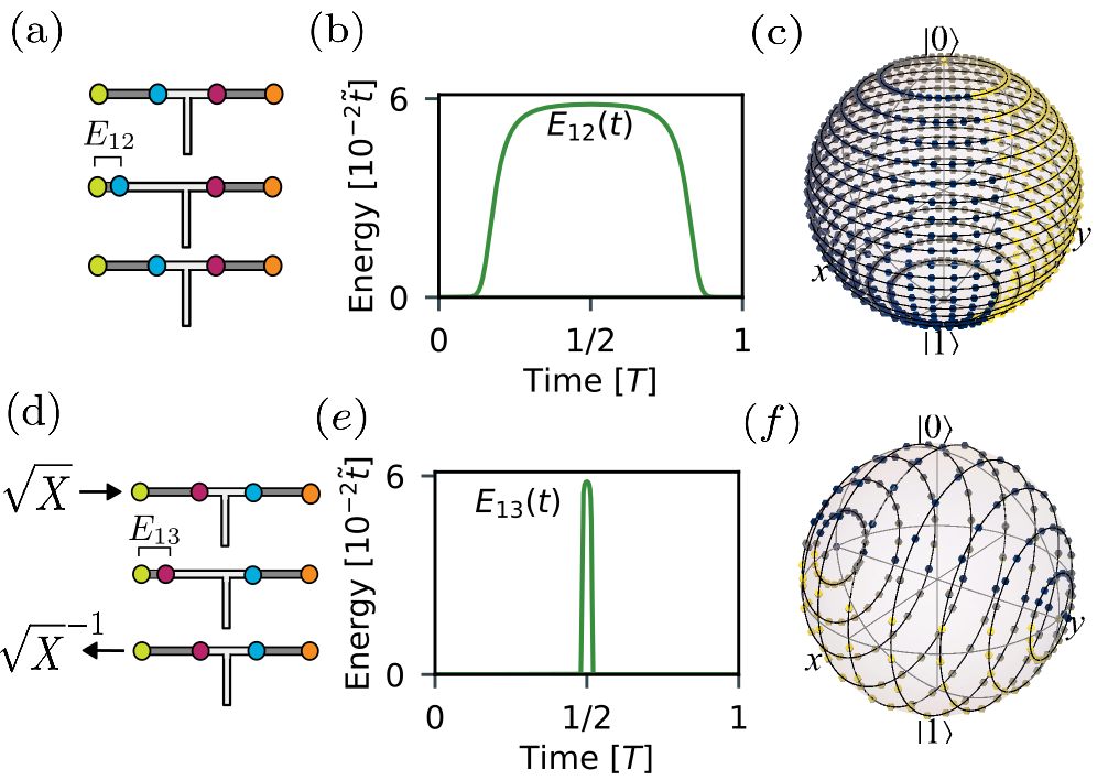
Figure 3: Single-Qubit gate simulations: (a) Schematics of $R_{z}(\theta)$-gate protocol. (b) Real-time instantaneous MZM energy during phase gate protocol. (c) Simulation of phase gate for different states $|\psi\rangle$ with varying $\theta\in[0,\pi]$ and fixed $\phi=0$. (d) Schematics of $R_{y}(\theta)$ gate protocol. (e) Real-time instantaneous MZM energy during $R_{y}(\theta)$ procedure. (f) Simulation of $R_{y}(\theta)$ gate with $\theta=\pi$ and varying $\phi\in[0,2\pi]$. Parameters for both simulations: ($\mu_{\textrm{topo}}$, $\mu_{\textrm{triv}}$, $r_{12}$, $r_{34}$, $L$)=$(0.35,10,10a_{0},10a_{0},20)$ with $\Delta r=8a_{0}$, $a_{0}$ being the lattice spacing.

Qubit gates I: Phase gate.— We now utilise these findings for the purpose of implementation and simulation of single-qubit gates using hybridization, essential for the successful operation of a universal quantum computer. All qubit gates considered will be conducted in the energy splitting regime where tunneling between $\gamma_{2}$ and $\gamma_{3}$ have been suppressed.

We begin with the $R_{z}(\varphi)$ gate, encompassing an arbitrary rotation by $\varphi$ about the $z$-axis (i.e., $|1\rangle_{\textrm{log}}\to e^{i\varphi}|1\rangle_{\textrm{log}}$). For $\varphi=\pi/4$, this is the T-gate, necessary for a full mapping onto the Bloch-sphere and unattainable via usual braiding procedures Bravyi and Kitaev (2002); Bonderson et al. (2010). The routine utilised is shown in Fig. 3 a, where we induce an energy splitting by dynamically moving $\gamma_{2}$ towards $\gamma_{1}$ by a displacement $\Delta r$. Afterwards, we move them back to their initial positions, where the energy splitting is negligible. The dynamic energy $E_{12}(t)$ as a function of time $t$ during this process is given in Fig. 3 b; the phase accumulation again depends on the average energy splitting, with $\varphi=\bar{E}_{12}T$, clockwise from the positive $x$-axis. The phase may then be set by controlling the protocol time $T$. This is displayed in Fig. 3 b, where a state with arbitrary initial $\hat{\sigma}_{z}$ projection, $\langle\hat{\sigma}_{z}\rangle=\textrm{cos}(\frac{\theta}{2})$, will map around the $xy$-plane for fixed $\theta$ by simply changing the protocol time $T$, corresponding to a controlled rotation about the $z$-axis.

We extend this to an arbitrary rotation about the y-axis, an $R_{y}(\varphi)$ gate. This is achieved by the routine $R_{y}(\varphi)=\sqrt{\textrm{X}}^{-1}R_{z}(\varphi)\sqrt{\textrm{X}}$, where the wavefunction overlap between $\gamma_{1}$ and $\gamma_{3}$ dictates the phase accumulation. The routine for this is depicted in Fig. 3 d, with the real time energy coupling $E_{13}(t)$ gained after the first $\sqrt{\textrm{X}}$ gate given in Fig. 3 e. As demonstrated in Fig. 3 (f), for an arbitrary state the $\langle\hat{\sigma}_{y}\rangle$ remains fixed as the state rotates about the $y$-axis with phase $\varphi=\bar{E}_{13}T$, clockwise from the positive $z$ axis. This constitutes enough for an arbitrary mapping of any state $|\psi\rangle$ onto the Bloch-sphere, as we may decompose an arbitrary rotation about the Bloch-sphere, into a set of Euler rotations. The trajectories using Eqs. (7-9) match numerical simulations with error up to $10^{-3}$. We may also analyse the $R_{x}(\varphi)$ gate, an arbitrary rotation about the $x$-axis, see SM.

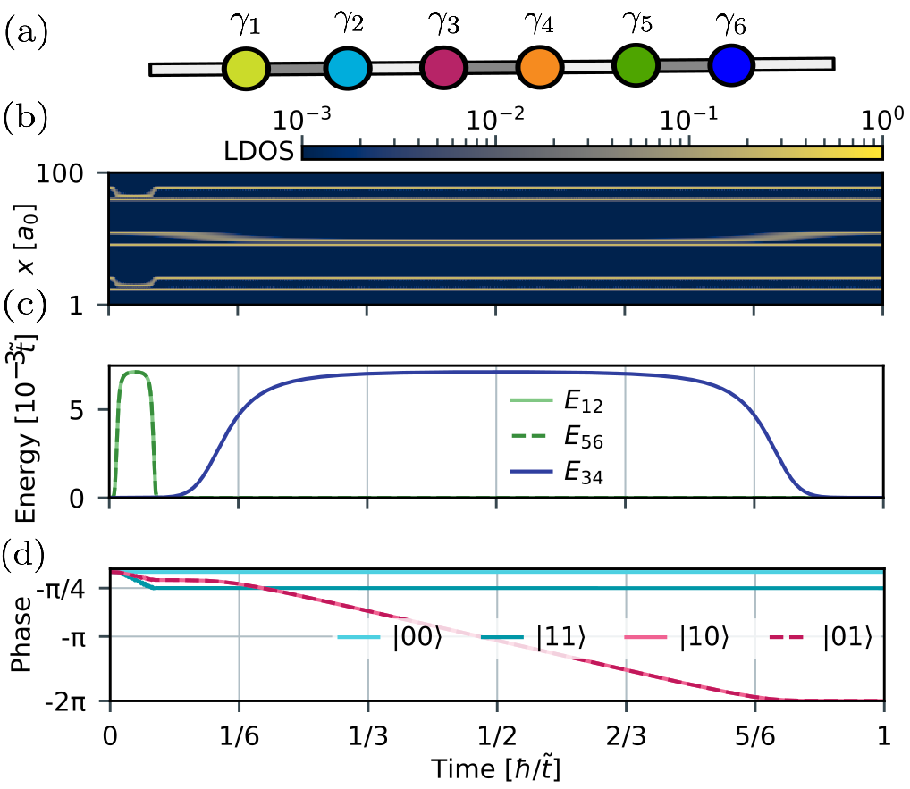
Figure 4: CT-gate via hybridization. (a) Kitaev chain with three topological segments and three pairs of MZMs. (b) LDOS over time $t$ in the ground-state manifold. (c) Plot of instantaneous energies as a function of real time $t$ for each Majorana state. (d) Plot of the phase evolution as a function of time for each basis state in the ground-state subspace. Parameters used: ($\mu_{\textrm{topo}}$, $\mu_{\textrm{triv}})$ =$(0.4,12)$ with $r_{12}$=$r_{34}$=$r_{56}$=$10a_{0}$ and $r_{23}$=$r_{45}$=$20a_{0}$. Chain length $L=100a_{0}$.

Qubit gates II: Controlled-Phase gate.— Finally, we extend phase-gate results to implement a two-qubit controlled phase gate, purely through hybridization of MZMs. Since this requires no braids, we remove the bottom leg of the T-junction and utilise a 1D-quantum wire with fixed superconducting phase $\phi_{p}=0$ Kitaev (2001), as shown in Fig. 4 a. In this case, using the dense qubit design Sarma et al. (2015) we initialise the system with three MZMs instead of two, with $|\psi\rangle=c_{1}|000\rangle_{\textrm{phys}}+c_{2}|110\rangle_{\textrm{phys}}+c_{3}|101\rangle_{\textrm{phys}}+c_{4}|011\rangle_{\textrm{phys}}$. For an arbitrary phase $\varphi$, a successful controlled phase gate is achieved by mapping $|101\rangle_{\textrm{phys}}\to e^{i\varphi}|101\rangle_{\textrm{phys}}$, leaving the other states unchanged. As shown in Fig. 4 (b, c), this may be achieved through a hybridization routine by inducing an energy splitting through the topological region by bringing $\gamma_{2}$ ($\gamma_{6}$) towards $\gamma_{1}$ ($\gamma_{5}$), inducing an average energy splitting $\bar{E}_{12}$ ($\bar{E}_{56}$). A state $|nlm\rangle_{\textrm{phys}}$ will subsequently map to $e^{-i(n\varphi_{12}+l\varphi_{34}+m\varphi_{56})}|nlm\rangle_{\textrm{phys}}$, with $n,l,m\in\{0,1\}$ indexing the occupation of the single-particle states $|\psi^{p}_{ij}(t)\rangle$, and $\varphi_{ij}=-\bar{E}_{ij}T_{ij}$ the accumulated phase of that state over a time $T_{ij}$. For an arbitrary choice of $\varphi$, we set $\bar{E}_{12}T_{12}=\varphi/2$ and $\bar{E}_{56}T_{56}=\varphi/2$, leading to a total accumulation of $\varphi$ on the state $|101\rangle_{\textrm{phys}}$, as necessary. To avoid a phase accumulation on $|110\rangle_{\textrm{phys}}$, $|011\rangle_{\textrm{phys}}$, $\bar{E}_{34}T_{34}=2\pi-\varphi$, leading to a total phase accumulation of $2\pi$ on these states, mapping them back to themselves. Setting $\varphi=-\pi/4$, where for fixed $\bar{E}_{12}=\bar{E}_{34}=\bar{E}_{56}=4.35\times 10^{-3}$, we set the total braid time $T_{12}=T_{56}=40.60\hbar$ and $T_{34}=609.06\hbar$. This is simulated in real time, as shown in Fig. 4 (d), where we track the phase accumulated on each state over time. For the $|101\rangle_{\textrm{phys}}$ state plateau at $t=T_{12}$ at $\pi/4$, as required for a controlled-T (CT) or controlled magic gate. As we allow the $\gamma_{3}$-$\gamma_{4}$ pairing to continue hybridizing, $|110\rangle_{\textrm{phys}}$ and $|011\rangle_{\textrm{phys}}$ continue accumulating a phase until they plateau at $\varphi=-2\pi$, leading to no change in these states. This constitutes the successful simulation of a CT-gate in a full dynamical process, purely through hybridization, on a Majorana-based platform, unattainable purely through braiding processes.

Outlook.— While key results have been restricted to a set of key gates, the methodology used may, in essence, be applied to construct and analyse the effects of hybridization on any arbitrary single-qubit gate. We emphasize that these results are platform independent. It provides, not only an accessible pathway to analyse Pauli qubit-error in any time-dependent process which hosts MZMs, essential for the experimental success of a braiding process, but also to control the hybridization for the implementation of quantum gates. This presents an advantage not just in terms of mitigating the effects of Pauli-qubit errors, but also on the mission to achieving a universal set of quantum gates for topological quantum computing.