Abstract

Efficient deployment of neural networks (NN) requires the co-optimization of accuracy and latency. For example, hardware-aware neural architecture search has been used to automatically find NN architectures that satisfy a latency constraint on a specific hardware device. Central to these search algorithms is a prediction model that is designed to provide a hardware latency estimate for a candidate NN architecture. Recent research has shown that the sample efficiency of these predictive models can be greatly improved through pre-training on some training devices with many samples, and then transferring the predictor on the test (target) device. Transfer learning and meta-learning methods have been used for this, but often exhibit significant performance variability. Additionally, the evaluation of existing latency predictors has been largely done on hand-crafted training/test device sets, making it difficult to ascertain design features that compose a robust and general latency predictor. To address these issues, we introduce a comprehensive suite of latency prediction tasks obtained in a principled way through automated partitioning of hardware device sets. We then design a general latency predictor to comprehensively study (1) the predictor architecture, (2) NN sample selection methods, (3) hardware device representations, and (4) NN operation encoding schemes. Building on conclusions from our study, we present an end-to-end latency predictor training strategy that outperforms existing methods on 11 out of 12 difficult latency prediction tasks, improving latency prediction by 22.5% on average, and up to to 87.6% on the hardest tasks. Focusing on latency prediction, our HW-Aware NAS reports a $5.8\times$ speedup in wall-clock time. Our code is available on https://github.com/abdelfattah-lab/nasflat_latency.

1 Introduction

With recent advancements in deep learning (DL), neural networks (NN) have become ubiquitous, serving a wide array of tasks in different deployment scenarios. With this ubiquity, there has been a surge in the diversity of hardware devices that NNs are deployed on. This presents a unique challenge as each device has its own attributes and the same NN may exhibit vastly different latency and energy characteristics across devices. Therefore, it becomes pivotal to co-optimize both accuracy and latency to meet stringent demands of real-world deployment Tan et al. (2019); Cai et al. ; Wu et al. (2019); Xu et al. (2020); Cai et al. (2020); Wang et al. (2020). The simplest way to include latency optimization is to profile the latency of a NN on its target device. However, this becomes costly and impractical when there are multiple small changes performed on the NN architecture either manually, or automatically through neural architecture search (NAS) Benmeziane et al. (2021). Not to mention that hardware devices are often not even available, or their software stacks do not yet support all NN architecture variants Elsken (2023), making it impossible to perform hardware-aware NN optimizations. For these reasons, much research has investigated statistical latency predictors that can accurately model hardware device latency with as few on-device measurements as possible.

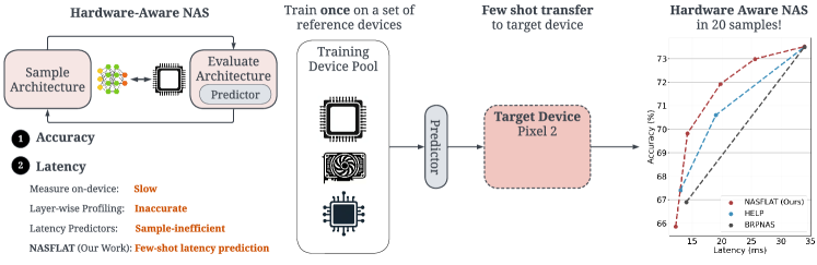
Figure 1: Predictors are central to hardware-aware neural architecture search, as they enable quick evaluation of candidate architectures. Latency predictors require several samples for training, but can be made more sample-efficient by first pre-training on a set of training devices. With the appropriate end-to-end latency predictor training pipeline, we can have extremely sample-efficient HW-Aware NAS!

Early work has used FLOPs as a proxy for latency Yu et al. (2020), while others created layerwise latency models Cai et al. . However, both of these approaches generally performed poorly and could not adequately represent end-to-end device latency. More recent work has used using Graph Convolutional Networks (GCNs) Dudziak et al. (2020) with much higher success in predicting the latency of NN architectures. However, a large number of NN latency samples needed to be gathered from each device for accurate modeling. To mitigate this, HELP Lee et al. (2021b) and MultiPredict Akhauri & Abdelfattah (2023) leverage transfer learning to train latency predictors with only a few NN latency samples. In this paradigm, a predictor is first trained to predict latency on a large set of training devices (the training stage), and then through few-shot meta-learning, fine-tuned to predict on a set of test devices (the transfer stage). This latter transfer stage can be performed efficiently using only a few sample measurements thus enabling the creation of latency predictors for new hardware devices in an inexpensive way. Figure 2 illustrates the training and transfer of few-shot latency predictors.

This new class of few-shot latency predictors has become very practical and attractive for use within NAS and other NN latency optimization flows. However, we have identified key shortcomings of existing works, as well as open research questions relating to the design of such predictors. First, the choice of the few NN latency samples for transferring a predictor are critical. Prior work has largely chosen this handful of NN architectures randomly but this often results in very high variance in predictive ability Lee et al. (2021b); Akhauri & Abdelfattah (2023). Simply put, the predictor performance is directly linked to the choice of those few samples. Second, multi-hardware latency predictors require an additional input that represents the hardware device for both the pretraining and transfer phases. One-hot encoding or a vector of latency measurements were used in the past for this purpose. Third, NN operations were represented in the same way across different devices even though different operations exhibit different properties inherent to each device’s hardware architecture and software compilation stack. Finally, the predictor architecture itself was largely reused from prior work Dudziak et al. (2020) without explicit modifications for multi-device hardware predictors. To address these main points, our work makes the following contributions:

1. We investigate and empirically test different NN sampling methods for few-shot latency predictors, demonstrating a 5% improvement compared to random sampling Lee et al. (2021b), while requiring no additional samples, unlike uniform latency sampling Nair et al. (2022).

2. We introduce hardware-specific NN operation embeddings to modulate NN encodings based on each hardware device, demonstrating a 7.8% improvement. We additionally investigate the impact of supplementing with unsupervised (Arch2Vec) Yan et al. (2020), computationally aware (CATE) Yan et al. (2021), and metric based (ZCP) Abdelfattah et al. (2021) encodings resulting in 6.2% improvement in prediction accuracy.

3. Drawing from our evaluations on 12 experimental settings, we present NASFLAT, Neural Architecture Sampler And Few-Shot Latency Predictor, a multi-device latency predictor architecture which combines our graph neural network with an effective sampler, supplementary encodings and transfer learning to deliver an average latency predictor performance improvement of 22.5%.

Our detailed investigation offers insights into effective few-shot latency predictor design, and results in improvements up to 87.6% on the most challenging prediction tasks (N2, FA, F2, F3 in Table 7), compared to prior work. Existing latency prediction tehniques often incur higher NAS costs owing to their sample inefficiency or complicated second-order transfer strategies. When evaluating end-to-end NAS outcomes, our approach demonstrates a $5.8\times$ speed-up in wall-clock time dedicated to latency predictor fine-tuning and prediction, compared to the best existing methods.

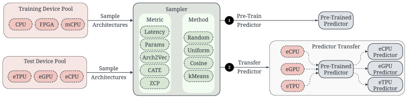
Figure 2: A few-shot latency predictor training pipeline. (1) We pre-train a predictor on a set of training devices. (2) The trained predictor can be adapted to any target device with just a few samples, using transfer learning. In this pipeline, the methodology used to sample neural networks as well as the predictor architecture play a key role.

2 Related Work

2.1 Hardware Latency Predictors

A good latency predictor can enable NAS to co-optimize latency and accuracy Tan et al. (2019); Cai et al. ; Wu et al. (2019); Xu et al. (2020); Cai et al. (2020); Wang et al. (2020). Latency prediction methods have evolved from early, proxy based methods such as FLOPs Yu et al. (2020) to learning-based methods. This is largely because such proxies often do not correlate strongly with latency at deployment. To get better estimates for latency, some works used layer-wise latency prediction methods by measuring the latency for each operation and summing up the operations that the neural network has via a look-up table Cai et al. . This method does not account for operation pipelining or other compiler optimizations that may take place when multiple layers are executed consecutively.

BRP-NAS Dudziak et al. (2020) takes into account such complexities and learns an end-to-end latency predictor which is trained on the target device. However, the latency measurements of a large number of NN architectures are required to perform well. This sample in-efficiency is largely because the latency predictor is trained from scratch. HELP Lee et al. (2021b) employs a pool of reference devices to train its predictor and utilizes meta-learning techniques to adapt this predictor to a new device. The transfer of a predictor from some source (training) devices to a target (test) device significantly improves the sample efficiency of predictors. MultiPredict Akhauri & Abdelfattah (2023) facilitates predictor transfer across search spaces through unified encodings based on zero-cost proxies or hardware latency measurements. Furthermore, MultiPredict investigates learnable hardware embeddings to represent different hardware devices within predictors. In our work, we extend the idea of a learnable hardware embedding to make it operation specific. Having a hardware embedding that explicitly interacts with the operation embeddings of a neural network architecture can capture intricacies in compiler level optimizations when executing hardware.

When transferring a predictor from a source device to a target device, the choice of samples used for few-shot learning plays a key role in the final performance. MAPLE-EdgeNair et al. (2022) investigates the impact of using the training device set latencies as reference for architecture to sample from the target device. For very large spaces, latencies of a sufficient diversity of neural network architectures may not be available even on the training devices. To address this, we look at methods of sampling a diverse set of neural networks from a target device which does not depend on latency or accuracy.

2.2 Encodings for NN representation

Early research in building predictors for accuracy and latency focused on using the adjacency and operation matrices to represent the directed acyclic graph (DAG) for the neural network architecture into a flattened vector to encode architectures White et al. (2020). HELP Lee et al. (2021b) and MultiPredict Akhauri & Abdelfattah (2023) use the flattened one-hot operation matrix for the FBNet space with a multi layer perceptron for the latency and accuracy predictor. BRPNAS Dudziak et al. (2020) employed a GCN with the adjacency-operation matrices as an input to build a latency and accuracy predictor for NASBench-201. More recently, works such as MultiPredict investigated the effect of capturing broad architectural properties by generating a vector of zero-cost proxies and hardware latencies to represent NNs. Additionally, there has been significant work in the field of encoding neural networks, notably the unsupervised learned encoding introduced in Arch2Vec Yan et al. (2020) which uses a graph auto-encoder to learn compressed latent representation for an NN architecture. Similarly, CATE Yan et al. (2021) leveraged concepts from masked language modeling to learn encodings for computationally similar architectures with a transformer.

In our work, we leverage these NN encodings to sample diverse architectures in the neural architecture search space. We also leverage these encodings to provide additional architectural information to our latency predictor.

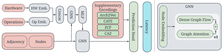
Figure 3: Our model architecture maintains separate operation and hardware embeddings which are concatenated and passed to a GNN to refine and contextualize the embeddings with respect to the overall neural architecture. This serves as the architecture embedding and is passed to another GNN along with the adjacency and node information. Optionally, supplementary encodings can be concatenated with the output of the GNN and fed to a prediction head to estimate the latency of the architecture.

3 Latency Predictor Design

3.1 Predictor Architecture

The design of the predictor itself plays a key role in improving sample efficiency of accuracy predictors in NAS. BRP-NAS Dudziak et al. (2020) used a GCN predictor to capture information about both the NN operations and connectivity. The same predictor has subsequently been used by HELP Lee et al. (2021b). TA-GATES Ning et al. (2022) further enhanced this predictor architecture with residual connections in the GCN module and a training-analogous operation update methodology, by maintaining a backward graph neural network module. This allows the iterative refinement of operation embeddings to provide more information about the architecture. We investigate the impact of these and other key components of predictor design in the Appendix, and design a latency predictor that accounts for both operation and hardware embeddings. We subsequently use this predictor for all experiments in this paper.

Figure 3 shows how we maintain separate embedding tables for the hardware device and operations. From our ablations in the Appendix, we find that a single GNN module to refine the operation embeddings is sufficient. To capture the complex interactions such as layer pipelining, operator fusion, we further incorporate the hardware embedding into each of the operation embeddings via concatenation. This joint embedding is then passed to a small operation GNN along with the adjacency and node embedding. Then, the embedding of the output node of the GNN is provided to an MLP which provides the hardware-operation joint embedding for the second (main) GNN used for modeling an input NN. Finally, supplementary encoding (discussed more below) can be concatenated with the GNN output and provided to a prediction head that can then output the latency metric.

3.2 GNN Module Design

Existing Graph Convolutional Networks (GCNs) experience an over-smoothing challenge, leading to a loss of discriminative information in the node embedding as aggregation layers increase. Addressing this, GATES Ning et al. (2023) introduced the Dense Graph Flow (DGF) module, which employs residual connections to maintain discriminative features across nodes. Furthermore, the Graph Attention (GAT) methodology, distinct from DGF, incorporates an attention mechanism during node aggregation. GAT evaluates node interactions through an attention layer. An operation attention mechanism, along with LayerNorm, refines information aggregation and ensures stable training, respectively. Further details of their implementation are in the Appendix. In our latency predictor, we use an ensemble of DGF and GAT modules.

3.3 Supplementary Encodings

Supplementary encodings are different ways to represent the input NN, and therefore may help contextualize the relations between a NN with respect to the entire search space. This can be useful for few-shot transfer of latency predictors. Learned encodings like Arch2Vec Yan et al. (2020), ZCP Akhauri & Abdelfattah (2023) and CATE Yan et al. (2021) provide distinct representations that allows them to effectively distinguish between various neural network (NN) architectures. For example, CATE (Yan et al., 2021) captures computational characteristics of NNs through its latent representations formed by computational clustering. Simultaneously, ZCP offers insights at the architectural level, acting as proxies that might correlate with accuracy.

To enhance the robustness and accuracy of our latency predictor, we integrate these encodings into its structure. Specifically, Arch2Vec, CATE, and ZCP encodings are introduced as supplementary inputs to the predictor head of our latency predictor. As illustrated in Figure 3, these encodings are fed into the MLP prediction head subsequent to the node aggregation phase. This augmentation not only incorporates the rich structural and computational characteristics of NN architectures but also helps the predictor to make better-informed latency estimates. In our experiments, we observed that incorporating architectural-level information from encodings can boost the sample-efficiency of our latency predictors. We also introduce the CAZ encoding, a combined representation formed by concatenating CATE, Arch2Vec, and ZCP, aiming to leverage the combined strengths of all three representations.

3.4 Transfer Of Pre-Trained Predictor

To pretrain the predictor, we form a large dataset from a number of source devices. This conventional training step is the same as prior work Lee et al. (2021b); Akhauri & Abdelfattah (2023). Once this pre-training phase is concluded, the subsequent step is the adaptation to a target hardware device. In alignment with the methodology described in MultiPredict Akhauri & Abdelfattah (2023), the predictor undergoes a fine-tuning process using the samples from the target device. The learning rate is re-initialized and fine-tuning of the predictor is conducted on the target device. We find that this is sufficient to calibrate the predictor to offer accurate latency estimates on the unseen device.

4 Neural Network Samplers

One of the key aspects of latency predictor training, especially in the low-sample count regime is choosing diverse neural networks. If all the samples profiled on the target device have similar computational characteristics, the predictor may not gather enough information to generalize. As depicted in Figure 2, one of the key aspects of predictor training and transfer is the sampler, which needs to select a diverse set of neural architectures to benchmark for few-shot learning. MAPLE-Edge Nair et al. (2022) uses latencies on a set of reference devices to identify architectures with distinct computational properties. While this is a very effective strategy to identify computationally distinct neural networks, this requires a very large number of on-device latency measurements—a key parameter that we would like to minimize.

In this section, we investigate methods of encoding NN architectures. We look at the impact of these encodings in helping us sample more diverse architectures. One key benefit of using these encodings to sample diverse architectures is that we no longer depend on reference device latency measurements.

4.1 Neural Network Encodings

A foundational aspect of hardware-aware NAS is to optimize an objective function $\ell:A\rightarrow\mathbb{R}$, where $\ell$ can quantify several performance metrics such as accuracy, latency, energy Dudziak et al. (2020). $A$ represents the NN search space, and architectures $a\in A$ can be represented as adjacency - operation matrices White et al. (2020). There are several methods that introduce alternative methods to represent $a$ Yan et al. (2020; 2021); Akhauri & Abdelfattah (2023). In this section, we look at some of these methods of encoding neural networks.

Learned encodings aim to represent the structural properties of a neural architecture in a latent vector without utilizing accuracy. Arch2Vec Yan et al. (2020) uses a variational graph isomorphism autoencoder to learn to regenerate the adjacency-operation matrix. CATE Yan et al. (2021) introduces a transformer that uses computationally similar architecture pairs (clustered by similar FLOPs or parameter count) to learn encodings. Naturally, the CATE encoding clusters architectures that have similar computational properties.

Zero-Cost Proxies (ZCP) encode neural networks as a vector of metrics. Each of these metrics attempt to encode properties of a neural network that may correlate with accuracy. Distinct connectivity patterns and operation choices (via varying adjacency-operation matrices) would initialize NNs that exhibit varied accuracy and latency characteristics. Thus, ZCP can implicitly capture architectural properties of neural networks, but does not contain explicit structural information.

4.2 Encoding-based Samplers

Encodings like ZCP, Arch2Vec, and CATE condense a broad spectrum of architectural information into a latent space. While Arch2Vec compresses the adjacency-operation matrix, capturing its intrinsic structure, CATE identifies and groups computationally similar architectures. In contrast, ZCPs capture global properties of the neural network that may correlate with accuracy or may encode operator level information about the architecture. Such encodings, collectively contain a rich representation of the entire neural architecture design space which can be used to decide which architectures to obtain the latency for on the target device.

For the ZCP encoding, we use 13 zero cost proxies, and generate 32-dimensional vectors for the Arch2Vec and CATE encodings. We further introduce an encoding ‘CAZ’, which combines the CATE, Arch2Vec and ZCP. Given the richness and diversity of the encoded representation of neural architectures, a systematic approach to selection becomes essential. We thus investigate two methodologies of using the encoding to identify architectures to sample for few-shot transfer to a target device.

Cosine Similarity and KMeans Clustering: Through our framework, we leverage cosine similarity Lahitani et al. (2016)—an intuitive metric of vector similarity—to discern architectures that may have distinct properties. Focusing on structures with reduced average cosine similarities ensures a wider design space coverage, potentially identifying ‘outlier’ architectures. Concurrently, utilizing the KMeans clustering algorithm MacQueen et al. (1967), we categorize encoded vectors into distinct groups, and opt for the one closest to the centroid of each cluster. The rationale is that these architectures are most representative of their respective clusters and hence provide a good spread across the design space.

5 Hardware Embeddings

HELP and MultiPredict Lee et al. (2021b); Akhauri & Abdelfattah (2023) investigate different methods of representing hardware, as an assigned device index, a vector of architectural latency measurements, or as a learnable hardware embedding table, which is relayed to the predictor for identifying devices. However, such an approach potentially oversimplifies the intricate dynamics of neural network deployment on hardware, thereby introducing the need for an interaction between the operation and hardware embedding. In this section, we discuss a methodology to initialize and utilize hardware embeddings to better model the dynamics of the target hardware.

Algorithm 1 Methodology to partition device sets.

  Input: Graph $G$ (negative correlations), integers $m$, $n$

  Output: Modified graph $B$

  $b\_m,b\_n=\texttt{kernighan-lin(G)}$

  {Initialize bipartite graph with correlations}

  $B=\texttt{initBipartite}(b\_m,b\_n,\texttt{correlations})$

  while len(B[0]) $\neq$ m or len(B[1]) $\neq$ n do

     {Identify disjoint device sets $U$ and $V$}

     $\texttt{l, r}=\texttt{B[0], B[1]}$

     {Remove node with highest correlation.}

     if len(B[0]) $>$ m then

        removeMaxWeightNode(B, l)

     end if

     if len(B[1]) $>$ n then

        removeMaxWeightNode(B, r)

     end if

  end while

5.1 Operation Specific Hardware Embedding

From a hardware perspective, the location of an operation in relation to its preceding and succeeding layers can considerably influence overall latency. This can be attributed to optimizations such as layer pipelining, where operations are organized in a staggered manner to maximize hardware utilization. Additionally, optimizations such as layer fusion which combine adjacent layers to streamline computations further underscore the importance of operation placement.

The latency predictor accepts the adjacency matrix, node, and operation indices as its inputs. The operation index is utilized to retrieve a learnable operation embedding from an embedding table, which encodes the properties and behaviors of the respective operation, however, when modeling latencies for various hardware devices, this singular operation embedding might not fully capture the nuances of each hardware. As depicted in Figure 3, we concurrently incorporate hardware-specific embeddings into our predictor, such that we are able to model the interaction between an operation and the hardware depending on its nature and position. Thus, the operation-specific hardware embedding introduces a more granular approach wherein each operation within the neural network is concatenated with a specific hardware embedding from an embedding table. Such a strategy not only encapsulates the intrinsic characteristics of the operation but also embeds information regarding how that specific operation would behave on the given hardware.

Table 1: Device sets for NASBench-201 and FBNet. S, T indicate source and target device pools respectively. Each device pool may contain more than one device, full details in the Appendix. Unless otherwise specified, we report the average correlation and standard deviation across trials and target (T) devices.

Devices

NB201

FBNet

ND

N1

N2

N3

N4

NA

FD

F1

F2

F3

F4

FA

DSP

-

-

T

-

-

-

-

-

-

-

-

-

CPU

ST

-

-

S

S

ST

ST

S

S

-

S

T

GPU

ST

T

S

T

T

S

ST

S

T

T

ST

S

FPGA

T

-

-

-

-

-

-

T

S

S

-

-

ASIC

T

S

-

S

S

T

-

T

-

-

S

-

eTPU

-

S

T

-

S

T

-

-

-

-

-

-

eGPU

-

-

T

S

S

-

-

-

-

-

-

-

eCPU

T

-

T

-

-

-

S

T

-

-

S

-

mGPU

-

S

-

S

S

-

-

-

-

-

-

-

mCPU

S

S

-

-

S

S

-

S

S

S

ST

T

mDSP

-

-

-

S

S

-

-

-

-

-

-

-

Table 2: The impact of operation-wise hardware embedding (OPHW) and hardware embedding initialization (INIT) on latency predictor performance. Both optimizations consistently demonstrate an improvement.

OPHW	ND	N1	N2	N3	N4	NA	FD	F1	F2	F3	F4	FA
✗	$0.804_{0.026}$	$0.701_{0.056}$	$0.763_{0.044}$	$0.680_{0.042}$	$0.757_{0.061}$	$0.660_{0.030}$	$0.839_{0.010}$	$0.753_{0.031}$	$0.745_{0.081}$	$0.685_{0.085}$	$0.813_{0.030}$	$0.566_{0.081}$
✓	$0.806_{0.038}$	$0.719_{0.050}$	$0.795_{0.034}$	$0.704_{0.058}$	$0.753_{0.052}$	$0.664_{0.059}$	$0.845_{0.009}$	$0.757_{0.048}$	$0.769_{0.076}$	$0.694_{0.076}$	$0.832_{0.026}$	$0.628_{0.103}$
INIT	ND	N1	N2	N3	N4	NA	FD	F1	F2	F3	F4	FA
✗	$0.794_{0.038}$	$0.701_{0.046}$	$0.791_{0.036}$	$0.718_{0.055}$	$0.750_{0.050}$	$0.658_{0.080}$	$0.707_{0.158}$	$0.609_{0.119}$	$0.754_{0.064}$	$0.655_{0.084}$	$0.659_{0.158}$	$0.559_{0.118}$
✓	$0.806_{0.038}$	$0.719_{0.050}$	$0.795_{0.034}$	$0.704_{0.058}$	$0.753_{0.052}$	$0.664_{0.059}$	$0.845_{0.009}$	$0.757_{0.048}$	$0.769_{0.076}$	$0.694_{0.076}$	$0.832_{0.026}$	$0.628_{0.103}$

Table 3: On over 10 out of 12 device sets, there is a benefit in using learned or zero-cost encodings for training-transfer sample selection.

Sampler	ND	N1	N2	N3	N4	NA
Latency (Oracle)	$0.929_{0.027}$	$0.960_{0.011}$	$0.793_{0.078}$	$0.951_{0.021}$	$0.919_{0.055}$	$0.851_{0.039}$
Random	$0.911_{0.038}$	$0.946_{0.026}$	$0.757_{0.052}$	$0.934_{0.032}$	$0.940_{0.026}$	$0.790_{0.070}$
Params	$0.898_{0.068}$	$0.934_{0.038}$	$0.767_{0.068}$	$0.918_{0.033}$	$0.940_{0.032}$	$0.801_{0.095}$
Arch2Vec	$0.912_{0.045}$	$0.931_{0.046}$	$0.741_{0.073}$	$0.930_{0.036}$	$0.907_{0.069}$	$0.849_{0.035}$
CATE	$0.893_{0.045}$	$0.937_{0.036}$	$0.761_{0.090}$	$0.935_{0.032}$	$0.945_{0.038}$	$0.767_{0.136}$
ZCP	$0.883_{0.075}$	$0.956_{0.039}$	$0.636_{0.170}$	$0.924_{0.051}$	$0.883_{0.071}$	$0.729_{0.212}$
CAZ	$0.925_{0.046}$	$0.957_{0.028}$	$0.761_{0.107}$	$0.935_{0.025}$	$0.866_{0.091}$	$0.680_{0.336}$
Sampler	FD	F1	F2	F3	F4	FA
Latency (Oracle)	$0.755_{0.048}$	$0.707_{0.052}$	$0.832_{0.035}$	$0.849_{0.022}$	$0.699_{0.077}$	$0.624_{0.112}$
Random	$0.665_{0.187}$	$0.642_{0.121}$	$0.801_{0.063}$	$0.809_{0.050}$	$0.658_{0.113}$	$0.615_{0.115}$
Params	$0.735_{0.073}$	$0.689_{0.070}$	$0.794_{0.078}$	$0.791_{0.062}$	$0.604_{0.239}$	$0.551_{0.146}$
Arch2Vec	$0.754_{0.071}$	$0.699_{0.046}$	$0.790_{0.065}$	$0.782_{0.083}$	$0.739_{0.054}$	$0.631_{0.169}$
CATE	$0.663_{0.132}$	$0.692_{0.079}$	$0.778_{0.078}$	$0.780_{0.076}$	$0.645_{0.118}$	$0.552_{0.147}$
ZCP	$0.744_{0.060}$	$0.665_{0.111}$	$0.789_{0.069}$	$0.801_{0.055}$	$0.734_{0.051}$	$0.586_{0.161}$
CAZ	$0.696_{0.107}$	$0.635_{0.105}$	$0.808_{0.040}$	$0.732_{0.097}$	$0.626_{0.127}$	$0.557_{0.141}$

5.2 Hardware Embedding Initialization

When adding a new target device, a good initialization for its hardware embedding is critical. For this, we gauge the computational correlation of the target device latency with each of the training devices. By identifying the training device with the highest correlation, we can use its learned hardware embedding as the starting point for the target device. This method harnesses latency similarities between devices, providing a good initialization for predictions on the target device. In addition, it avoids a cold start when using the predictor for a new device, allowing the predictor to be functional with just a small number of latency samples on the new device.

6 Experiments

Table 4: Over three device sets on two NAS spaces, there is a benefit in using supplementary encodings for representing neural networks.

Encoding	ND	N1	N2	N3	N4	NA
AdjOp	$0.959_{0.018}$	$0.971_{0.010}$	$0.848_{0.063}$	$0.966_{0.006}$	$0.965_{0.012}$	$0.893_{0.029}$
(+ Arch2Vec)	$0.961_{0.010}$	$0.972_{0.007}$	$0.816_{0.065}$	$0.968_{0.005}$	$0.965_{0.009}$	$0.895_{0.035}$
(+ CATE)	$0.954_{0.022}$	$0.962_{0.029}$	$0.833_{0.072}$	$0.967_{0.007}$	$0.967_{0.008}$	$0.907_{0.024}$
(+ ZCP)	$0.955_{0.024}$	$0.968_{0.014}$	$0.855_{0.026}$	$0.963_{0.009}$	$0.962_{0.011}$	$0.896_{0.018}$
(+ CAZ)	$0.960_{0.014}$	$0.972_{0.005}$	$0.861_{0.036}$	$0.965_{0.005}$	$0.966_{0.006}$	$0.899_{0.012}$
Encoding	FD	F1	F2	F3	F4	FA
AdjOp	$0.783_{0.035}$	$0.744_{0.032}$	$0.855_{0.021}$	$0.850_{0.026}$	$0.750_{0.066}$	$0.694_{0.060}$
(+ Arch2Vec)	$0.881_{0.016}$	$0.788_{0.027}$	$0.878_{0.020}$	$0.890_{0.012}$	$0.848_{0.020}$	$0.723_{0.034}$
(+ CATE)	$0.837_{0.031}$	$0.744_{0.037}$	$0.839_{0.022}$	$0.845_{0.037}$	$0.805_{0.023}$	$0.678_{0.055}$
(+ ZCP)	$0.960_{0.008}$	$0.842_{0.020}$	$0.895_{0.018}$	$0.899_{0.019}$	$0.843_{0.028}$	$0.776_{0.038}$
(+ CAZ)	$0.899_{0.021}$	$0.783_{0.033}$	$0.842_{0.036}$	$0.852_{0.029}$	$0.761_{0.056}$	$0.683_{0.077}$

In this section, we systematically investigate key design considerations for predictor design. We begin by looking at the effectiveness of our proposed operation specific hardware embedding as well as hardware embedding initialization. We further investigate the impact that graph neural network module design has on predictor efficacy, looking at graph convolutional networks, graph attention networks and their ensemble. We then study the impact of neural network encoding strategies on selection of neural network architectures for transferring predictors to a target device. By supplementing our predictor with additional NN encodings, we provide additional information coveying the relative performance of NNs within a search space—our ablation shows improved prediction. Finally, we combine our empirically-driven optimizations on sampling, encodings, hardware embeddings, and predictor architecture to design a state-of-the-art latency predictor. Our evaluation encompasses both the Spearman Rank Correlation of predicted latency and ground truth on multiple device sets, in addition to end-to-end HW-Aware NAS.

6.1 Designing Evaluation Sets

One of the key challenges in evaluating HW-Aware NAS is the lack of standardized evaluation sets and hardware latency data-sets. HW-NAS-Bench Li et al. (2021), HELP Lee et al. (2021b) and EAGLE Dudziak et al. (2020) collectively open-source latencies for a wide range of hardware on the NASBench-201 and FBNet design spaces, making HW-Aware NAS evaluation easier. However, MultiPredict identified an issue where device sets on which current latency predictors were evaluated on showed high training-test correlation. For NASBench-201 and FBNet, high training-test correlation device sets are denoted as ‘ND’ and ‘FD’, respectively. To this end, MultiPredict introduced device sets with low training-test correlation to evaluate latency predictors, indicated by ‘NA’ and ‘FA’ (A signifying the adversarial nature of the device set) in Table 1. A key shortcoming in these existing works is that the devices that the predictor is evaluated on is cherry-picked, exhibiting a high correlation between the training devices and test devices, a property that is not guaranteed in practice. To circumvent this limitation, we employ an automated algorithmic strategy to design training and test devices to maintain low mutual correlation. Initially, we compute the Spearman correlation of latencies between all available devices, and construct a graph structure with negative correlations between devices which serve as edge weights. As depicted in Algorithm 1, we then leverage the Kernighan-Lin Kernighan & Lin (1970) bisection method to bisect the graph, aiming to group devices with minimal intra-group correlation. We iteratively trim the bipartite graph to maintain a specified number of devices in each set. By algorithmically partitioning device sets, we ensure an objective and unbiased selection process. With this strategy, we introduce four device sets for NASBench-201 and FBNet, identified by (N1, N2, N3, N4) and (F1, F2, F3, F4) in Table 1.

6.2 Experimental Setup

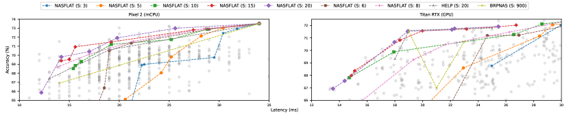
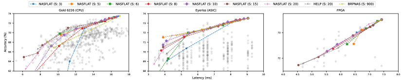
Figure 5: Latency-Accuracy NAS results for different sample sizes (S)

In each of our experiments, we pretrain our predictor on many samples from multiple source devices, then we fine-tune the predictor on only a few samples from the target devices as defined by our evaluation sets. We report the Spearman Rank Correlation Coefficient of predicted latency relative to ground-truth latency values as a measure of predictive performance. In Figure 5, we investigate the GAT and DGF GNN module. In all our experiments, we decide to use the DGF-GAT ensemble as the GNN module. The appendix details the precise experimental settings for each of our results.

Table 5: On NB201, GAT outperforms DGF. The difference is less evident on FBNet, we thus use an ensemble of DGF and GAT.

GNN Module	ND	N1	N2	N3
DGF	$0.814_{0.026}$	$0.741_{0.032}$	$0.802_{0.021}$	$0.710_{0.042}$
GAT	$0.965_{0.005}$	$0.848_{0.038}$	$0.612_{0.032}$	$0.762_{0.039}$
Ensemble	$0.965_{0.011}$	$0.829_{0.046}$	$0.634_{0.029}$	$0.789_{0.054}$
GNN Module	FD	F1	F2	F3
DGF	$0.844_{0.004}$	$0.740_{0.055}$	$0.752_{0.076}$	$0.621_{0.120}$
GAT	$0.823_{0.019}$	$0.749_{0.042}$	$0.700_{0.114}$	$0.589_{0.083}$
Ensemble	$0.835_{0.007}$	$0.733_{0.059}$	$0.766_{0.013}$	$0.609_{0.106}$

6.3 Hardware-aware Operation Embeddings

Instead of representing operations with a fixed embedding, we modulate embeddings based on each hardware device as described in Section 5. Table 2 evaluates the impact of this optimization on the predictive ability using our latency predictor. We find that on 11 out of 12 device pools, there is a positive impact of introducing the operation-wise hardware embedding. Additionally, we evaluate the impact of initializing the hardware embedding of the target device with the embedding of the most closely-correlated source device. Our results show consistent improvement from this initialization scheme as shown in Table 2. These two optimizations have empirically demonstrated their efficacy in utilizing hardware-specific operation embeddings, and mitigating new device cold start in our predictor.

Table 6: We study the impact of different design choices on the performance of predictors. Each row adds a feature and also inherits the design choices above it.

	F1	F2	F3	F4	N1	N2	N3	N4
Baseline Predictor	$0.603_{0.104}$	$0.800_{0.050}$	$0.792_{0.058}$	$0.502_{0.142}$	$0.938_{0.034}$	$0.781_{0.084}$	$0.907_{0.019}$	$0.922_{0.021}$
(+ HWInit)	$0.573_{0.114}$	$0.770_{0.072}$	$0.822_{0.053}$	$0.566_{0.127}$	$0.938_{0.031}$	$0.776_{0.039}$	$0.887_{0.087}$	$0.898_{0.046}$
(+ OpHW)	$0.610_{0.076}$	$0.801_{0.045}$	$0.824_{0.025}$	$0.549_{0.078}$	$0.949_{0.017}$	$0.821_{0.045}$	$0.938_{0.021}$	$0.955_{0.015}$
(+ Sampler)	$0.639_{0.069}$	$0.813_{0.042}$	$0.810_{0.053}$	$0.616_{0.116}$	$0.962_{0.012}$	$0.803_{0.067}$	$0.920_{0.034}$	$0.961_{0.007}$
(+ Supp. Encoding)	$0.727_{0.048}$	$0.844_{0.031}$	$0.816_{0.057}$	$0.796_{0.045}$	$0.936_{0.033}$	$0.812_{0.059}$	$0.930_{0.028}$	$0.940_{0.017}$

6.4 Encoding-based Samplers

Here, we evaluate different sampling methods, specifically those based on uniformly sampling NNs based on different encodings. Our findings in Table 3 present a somewhat varied pattern. While encodings-based samplers were advantageous in 10 out of 12 device pools, determining the optimal sampler became a complex task dependent on the each device pool. Notably, CATE’s performance was subpar, especially on FBNet. A potential reason for this could be the disparity between the FBNet search space, which possesses $9^{22}$ unique architectures, and the latency dataset available in HWNASBench, restricted to only $5000$ architectures. Consequently, when training the CATE encoding on this limited set, computationally similar architectures do not carry much meaning with respect to the entire FBNet search space. Arch2Vec is trained similarly, but since computationally similar architectures are not required, it is able to learn a representation on a smaller space.

Delving deeper into the selection strategy used for clustering the encodings, we observed a pronounced inclination towards the cosine similarity approach. As detailed in the appendix, Cosine consistently demonstrated superior performance over KMeans. Additionally, KMeans was occasionally unable to segment the space adequately to yield architectures (as evidenced by NaN entries).

6.5 Supplementary NN Encodings

Table 7: We train our predictor with our proposed sampler, GAT+GCN ensemble architecture, operation-wise hardware embedding, hardware embedding initialization, and report our end-to-end predictor transfer result (Spearman Rank Correaltion). On 11 out of 12 tasks, our predictor works best for NASBench-201 and FBNet respectively. Standard deviations are reported for results we produce in our paper.

	Source	Target	ND	NA	N1	N2	N3	N4	GM
	Samples
HELP	900	20	$0.948_{0.006}$	$0.410_{0.037}$	$0.604_{0.044}$	$0.509_{0.007}$	$0.729_{0.027}$	$0.746_{0.042}$	$0.634$
MultiPredict	900	20	$0.930_{0.012}$	$0.820_{0.019}$	$0.907_{0.003}$	$0.757_{0.045}$	$0.947_{0.012}$	$0.952_{0.011}$	$0.882$
NASFLAT	$25$	20	$0.959_{0.007}$	$0.893_{0.036}$	$0.967_{0.007}$	$0.857_{0.029}$	$0.962_{0.008}$	$0.959_{0.012}$	$0.931$
			FD	FA	F1	F2	F3	F4	GM
HELP	4000	20	$0.910$	$0.37$	$0.793_{0.028}$	$0.543_{0.036}$	$0.413_{0.015}$	$0.799_{0.004}$	$0.602$
MultiPredict	4000	20	$0.960$	$0.45$	$0.756_{0.026}$	$0.567_{0.075}$	$0.434_{0.040}$	$0.763_{0.011}$	$0.627$
NASFLAT	$800$	20	$0.961_{0.007}$	$0.577_{0.079}$	$0.809_{0.019}$	$0.871_{0.024}$	$0.814_{0.046}$	$0.734_{0.142}$	$0.784$

By inputting supplementary NN encodings in our predictor (as shown in Figure 3), we can better represent the relative performance of NNs, especially when only a few samples are used for predictor training. From Table 4, we see that the impact of these supplementary encodings revealed an almost universal benefit: 11 out of 12 device pools displayed improved performance. This is likely due to the fact that these encodings contextualize the few target samples with respect to the broader search space more effectively.

6.6 Impact of Pre-Training Samples

Focusing on the pre-training phase, we delve into how varying sample sizes from source devices influence the Spearman rank correlation. Notably, the end-to-end performance does not consistently improve with an increasing number of samples; quite the opposite, it occasionally diminishes. This counterintuitive phenomenon can be ascribed to a situation where the model, encountering a multitude of source devices that share high correlation, ends up overfitting to the specifics of this source device set. For instance, in ‘Task N4’, where the training set already has a relatively low average correlation between devices, degradation of predictive performance with more samples isn’t observed. However, in ‘Task N2’, which comprises solely of GPUs, this tendency becomes more clear. These findings indicate that the diversity in the training pool is important to benefit from larger source sample training sets. Merely increasing the number of samples without assuring their diversity can hinder predictor pre-training. We perform an ablation in the appendix to select a reasonable number of pretraining samples for use with our predictor in subsequent experiments.

6.7 Combining our Optimizations and a Comparison to Prior Work

Table 6 lists the effect of combining all of our optimizations including the hardware-aware operation embeddings, embedding initialization, encoding-based samplers, and supplementary encodings, all performed on our predictor architecture. We call our final predictor NASFLAT: Neural Architecture Sampler And Few-Shot Latency Predictor. On average, our first 3 optimizations bring marked improvements to the predictor performance. We also found that using our encoding-based samplers generally reduced variance, making predictor construction more reliable. This is further quantified in the appendix.

Finally, Table 7 incorporates all our optimizations to deliver state-of-the-art end-to-end latency predictor performance on 11 out of 12 device sets. We show that, especially on challenging tasks, our optimizations improve predictor accuracy by 22.5% on average, and up to 87.6% for the hardest (F3) task when compared to HELP Lee et al. (2021b).

Table 8: Performance comparison of different latency estimators combined with MetaD2A for latency-constrained NAS, on CIFAR-100 dataset with NAS-Bench-201 search space. For the building time and the total NAS cost of MetaD2A+HELP, we report only time and cost during the meta-test time. The meta-training time of HELP is 25 hours, NASFLAT is 25 minutes and the time to meta-train the MetaD2A is 46 GPU hours, which is conducted only once across all unseen devices. We report average over 10 trials. S indicates number of new samples on target device.

Device	Model	Const	Latency	Accuracy		Latency Model		Total NAS Cost	Speed Up
		(ms)	(ms)	(%)		Sample	Building Time	(Wall Clock)
	MetaD2A + BRP-NAS Dudziak et al. (2020)	14	14	66.9		900	1120s	1220s	0.1$\times$
	MetaD2A + HELP Lee et al. (2021b)		13	67.4		20	25s	125s	1$\times$
	MetaD2A + NASFLAT		$14.4_{3.41}$	$68.53_{3.04}$		20	25s	29.1s	4.3$\times$
Unseen Device	MetaD2A + BRP-NAS Dudziak et al. (2020)	22	34	73.5		900	1120s	1220s	0.1$\times$
Google Pixel2	MetaD2A + HELP Lee et al. (2021b)		19	70.6		20	25s	125s	1$\times$
	MetaD2A + NASFLAT		$22.2_{6.46}$	$72.08_{0.91}$		20	25s	29.1s	4.3$\times$
	MetaD2A + BRP-NAS Dudziak et al. (2020)	34	34	73.5		900	1120s	1220s	0.1$\times$
	MetaD2A + HELP Lee et al. (2021b)		34	73.5		20	25s	125s	1$\times$
	MetaD2A + NASFLAT		$34_{0.0}$	$73.5_{0.0}$		20	25s	29.1s	4.3$\times$
	MetaD2A + Layer-wise Pred.	18	37	73.2		900	998s	1098s	0.1$\times$
	MetaD2A + BRP-NAS Dudziak et al. (2020)		21	67.0		900	940s	1040s	0.1$\times$
	MetaD2A + HELP Lee et al. (2021b)		18	69.3		20	11s	111s	1 $\times$
	MetaD2A + NASFLAT		$17.10_{2.65}$	$69.92_{2.35}$		20	11s	15.4s	7.2$\times$
Unseen Device	MetaD2A + Layer-wise Pred.	21	41	73.5		900	998s	1098s	0.1$\times$
Titan RTX	MetaD2A + BRP-NAS Dudziak et al. (2020)		19	71.5		900	940s	1040s	0.1$\times$
(Batch Size 256)	MetaD2A + HELP Lee et al. (2021b)		19	71.6		20	11s	111s	1 $\times$
	MetaD2A + NASFLAT		$20.47_{2.46}$	$71.45_{0.45}$		20	11s	15.4s	7.2$\times$
	MetaD2A + Layer-wise Pred.	25	41	73.2		900	998s	1098s	0.1$\times$
	MetaD2A + BRP-NAS Dudziak et al. (2020)		23	70.7		900	940s	1040s	0.1$\times$
	MetaD2A + HELP Lee et al. (2021b)		25	71.8		20	11s	111s	1 $\times$
	MetaD2A + NASFLAT		$26.61_{4.84}$	$71.9_{0.87}$		20	11s	15.4s	7.2$\times$

6.8 Neural Architecture Search

To assess the performance on end-to-end NAS, our predictor is used within the hardware-aware NAS system presented in HELP Lee et al. (2021b). We use the same NAS system with Metad2a Lee et al. (2021a) as the NN search algorithm for accuracy, and our predictor to find latency. We evaluate our results using multiple metrics. Primarily, we consider the number of architecture-latency pair samples taken from the target device. These samples are crucial for constructing the latency predictor, which encompasses the total time span of sample acquisition, architecture compilation on the device and the latency measurement process. While this metric remains the same between our method and HELP, we also evaluated the total NAS cost, a combination of the time taken for few-shot transfer of predictor to the NAS experiment device, and the time spent on latency prediction during NAS. The results in Table 8 (and companion plots) demonstrate a consistent improvement in the discovered NNs, with the latency-accuracy Pareto curve dominating that of prior works in most cases. Additionally, our predictor is faster to invoke when compared to HELP, making fast NAS methods—such as Metad2a—around 5$\times$ faster.

7 Conclusion

In this paper, we systematically examined several design considerations inherent to hardware latency predictor design. We studied the influence of operation-specific hardware embeddings, graph neural network module designs, and the role of neural network encodings in enhancing predictor accuracy. Our exhaustive empirical evaluations across multiple device sets yielded key insights, such as the importance of sample diversity during pre-training and the significant impact of supplemental encodings based on their correlation with test devices. By adopting an objective algorithmic strategy for device set selection, we achieved a more unbiased view of latency predictor performance. Leveraging these insights, we developed and validated NASFLAT, a latency predictor that outperformed existing works in 11 of 12 device sets. Future endeavors to refine predictors could involve exploring sophisticated transfer learning techniques akin to HELP Lee et al. (2021b), deepening our understanding of neural network encodings’ mechanisms as samplers, and investigating various sampling methodologies. Our work paves the way for more reliable and efficient use of predictors, both within NAS, and more generally in the optimization of NN architectures.

Appendix A Supplemental Material

A.1 Best practices for NAS

(White et al., 2020; Li & Talwalkar, 2019; Ying et al., 2019; Yang et al., 2020) discuss improving reproducibility and fairness in experimental comparisons for NAS. We thus address the sections released in the NAS best practices checklist by (Lindauer & Hutter, 2019).

• Best Practice: Release Code for the Training Pipeline(s) you use: We release code for our Predictor, CATE, Arch2Vec encoder training set-up.

• Best Practice: Release Code for Your NAS Method: We do not conduct NAS.

• Best Practice: Use the Same NAS Benchmarks, not Just the Same Datasets: We use the NASBench-201 and FBNet datasets for evaluation. We also use a sub-set of Zero Cost Proxies from NAS-Bench-Suite-Zero.

• Best Practice: Run Ablation Studies: We run extensive ablation studies in our paper. We conduct ablation studies with different supplementary encodings in the main paper as well as predictor ablations in the appendix.

• Best Practice: Use the Same Evaluation Protocol for the Methods Being Compared: We use the same evaluation protocol as existing works in this field (HELP Lee et al. (2021b) and MultiPredict Akhauri & Abdelfattah (2023))

• Best Practice: Evaluate Performance as a Function of Compute Resources: In this paper, we study the sample efficiency of latency predictors. We report results in terms of the ’number of trained models required’. This directly correlates with compute resources, depending on the NAS space training procedure.

• Best Practice: Compare Against Random Sampling and Random Search: We propose a end-to-end predictor design methodology, not a NAS method.

• Best Practice: Perform Multiple Runs with Different Seeds: Our appendix contains information on number of trials and our tables in the main paper are with standard deviation.

• Best Practice: Use Tabular or Surrogate Benchmarks If Possible: All our evaluations are done on publicly available Tabular and Surrogate benchmarks.

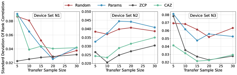
Figure 4: Standard deviation of neural network samplers using supplementary encodings are generally lower than random methods.

Table 9: In our tests, cosine based selection for samplers with vector encodings outperforms kMeans. Tested on Task N3 with operation-wise hardware embedding and hardware embedding initialization.

	10 Samples
NB201	ZCP	Arch2Vec	CATE	CAZ
Cosine	$0.948$	$0.949$	$0.933$	$0.951$
Kmeans	$0.729$	$0.670$	$0.826$	$0.892$
FBNet	ZCP	Arch2Vec	CATE	CAZ
Cosine	$0.822$	$0.803$	$0.805$	$0.788$
Kmeans	$0.412$	$0.657$	NaN	$0.718$
	20 Samples
NB201	ZCP	Arch2Vec	CATE	CAZ
Cosine	$0.963$	$0.960$	$0.952$	$0.960$
Kmeans	$0.786$	$0.680$	$0.885$	$0.948$
FBNet	ZCP	Arch2Vec	CATE	CAZ
Cosine	$0.845$	$0.839$	$0.828$	$0.852$
Kmeans	$0.818$	$0.812$	NaN	$0.835$

A.2 Experimental settings for tables

Table 1: Random seeds are used to generate 4 different device sets for NB201 and FBNet each.
Table 2 uses Random sampler without supplementary encoding, 20 samples on the target device. No supplementary encoding is used.
Table 3: only 5 samples on the test device are used for transfer to effectively test different samplers under few-shot conditions. No supplementary encoding is used.
Table 4: CAZ + kMeans was used as the sampler and 20 samples are fetched for transfer to ensure effective training of baseline predictor.
Table 5: 20 samples are used for transfer with random sampler, no supplementary encoding.
Table 7: Predictor is trained with the CAZ and CATE sampler with ZCP and Arch2Vec supplemental encoding for NASBench-201 and FBNet respectively.
Table 6: ZCP and Arch2Vec supplemental encoding, CAZ and CATE sampler for NASBench-201 and FBNet respectively. 20 samples used for transfer to target device.

A.3 NAS Search Spaces

Latency predictors for neural architecture search (NAS) generally operate on a pre-defined search space of neural network architectures. Several such architecture search spaces can be represented as cells where nodes represent activations and edges represent operations. In this paper, we evaluate a wide range of hardware devices across 11 representative platforms described in Table 1 on two neural architecture search spaces, NASBench-201 and FBNet. The hardware latency data-set generated for our tests is collated from HW-NAS-Bench Li et al. (2021) and Eagle Dudziak et al. (2020).

Micro Cell Space (NASBench-201) Dong & Yang (2020) is a cell-based architecture design with each cell comprising 4 nodes and 6 edges. Edges can have one of five types: zerorize, skip-connection, 1$\times$1 convolution, 3$\times$3 convolution, or 3$\times$3 average-pooling. With 15625 unique architectures, the entire network is assembled using a stem cell, three stages of five cell repetitions, followed by average-pooling and a final softmax layer.

Macro Cell Space (FBNet) Wu et al. (2019) features a fixed macro architecture with a layer-wise search space. It offers 9 configurations of ’candidate blocks’ across 22 unique positions, leading to approximately $10^{21}$ potential architectures. Despite its macro nature, FBNet can be cell-represented with 22 operational edges. For consistency, we model both NASBench-201 and FBNet using adjacency and operation matrices.

A.3.1 GNN Module Design

Despite the improved performance that GCNs can deliver, they suffer from an over-smoothing problem Ming Chen et al. (2020), where this is a gradual loss of discriminative information between nodes due to the convergence of node features across multiple aggregation layers. To this end, GATES Ning et al. (2023; 2022) introduced a custom GCN module referred to as Dense Graph Flow (DGF), which utilizes residual connections within the DGF to improve performance. Additionally, we study another node propagation mechanism based on graph attention.

Dense Graph Flow (DGF): The Dense Graph Flow (DGF) module implements residual connections to retain localized, discriminative features. To describe this mathematically, consider $X^{l}$ as the input feature matrix for layer $l$, $A$ as the adjacency matrix, and $O$ as the operator embedding. The corresponding parameters and bias terms for this layer are represented by $W^{l}_{o}$, $W^{l}_{f}$, and $b^{l}_{f}$. Using these, the input feature matrix for the subsequent layer, $X^{l+1}$, is determined using the sigmoid activation function, $\sigma$, as:

$$X^{l+1}=\sigma(OW^{l}_{o})\odot(AX^{l}W^{l}_{f})+X^{l}W^{l}_{f}+b^{l}_{f}$$ (1)

Graph Attention (GAT): The GAT approach (Veličković et al., 2018) distinguishes itself from DGF by its attention mechanism during node information aggregation. Rather than utilizing a linear transformation $W^{l}_{o}$ like in DGF for operation features, GAT assesses pairwise interactions among nodes via its dedicated attention layer. For layer $l$, node features (or input feature matrix) are denoted by $X^{l}$. A linear transformation characterized by the projection matrix $W^{l}_{p}$ uplifts the input to advanced features. Subsequently, node features undergo self-attention via a common attentional mechanism, denoted as $a$. $S$ refers to SoftMax and $L$ refers to LeakyReLU. Hence, the output $X^{l+1}$ is formulated as:

$$\text{Attn}_{j}(X^{l})=\text{S}(\text{L}(A_{j}\cdot a(W^{l}_{p}X^{l}\odot W_{p}X^{l}_{j})))\odot W_{p}X^{l}_{j}$$ (2)

$$X^{l+1}=\text{LayerNorm}\left(\sigma(OW^{l}_{o})\odot\sum_{j=1}^{n}\text{Attn}_{j}(X^{l})\right)$$ (3)

Here, $\text{Attn}_{j}$ represents the normalized attention coefficients, and $\sigma$ is the sigmoid activation function. To enhance GAT’s efficacy, we integrate the learned operation attention mechanism $W_{o}$ (as mentioned in Equation 1) with pairwise attention. This combined attention scheme fine-tunes the aggregated information. Additionally, we incorporate LayerNorm to ensure training stability.

A.4 Predict Design Ablation

In this subsection, we conduct an in-depth study of predictor design inspired by recent research, but from an accuracy maximization perspective. We use our ablation on accuracy to design a state-of-the-art predictor that we use for our latency study. To achieve a fair evaluation, we test each design improvement on a huge set of neural architecture design spaces detailed below.

Figure 6: A study investigating the effect of number of latency samples per training (source) device and its impact on predictor performance. We use 20 samples from the target device.

Space	Amoeba		DARTS		ENAS		ENAS_fix-w-d		NASNet		PNAS		nb101		nb201
All Node Encoding	False	True	False	True	False	True	False	True	False	True	False	True	False	True	False	True
Samples
8	0.100	0.078	0.079	0.076	0.075	0.078	0.183	0.154	0.135	0.122	0.082	0.089	0.395	0.370	0.445	0.533
16	0.202	0.157	0.178	0.184	0.165	0.186	0.322	0.302	0.155	0.127	0.124	0.127	0.448	0.350	0.647	0.656
32	0.287	0.293	0.246	0.251	0.295	0.277	0.319	0.301	0.223	0.223	0.246	0.251	0.543	0.532	0.709	0.715
64	0.375	0.367	0.416	0.411	0.364	0.357	0.374	0.372	0.347	0.331	0.348	0.330	0.652	0.623	0.771	0.762
128	0.455	0.419	0.476	0.474	0.463	0.442	0.386	0.388	0.432	0.398	0.505	0.494	0.703	0.698	0.818	0.808

Table 10: Investigating the impact of whether we should use the features of every node for the backward MLP (True) or not (False).

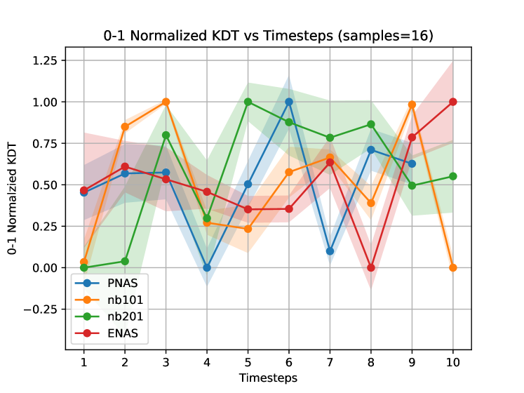
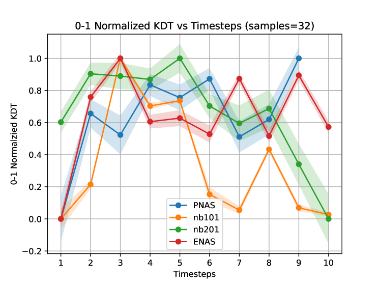
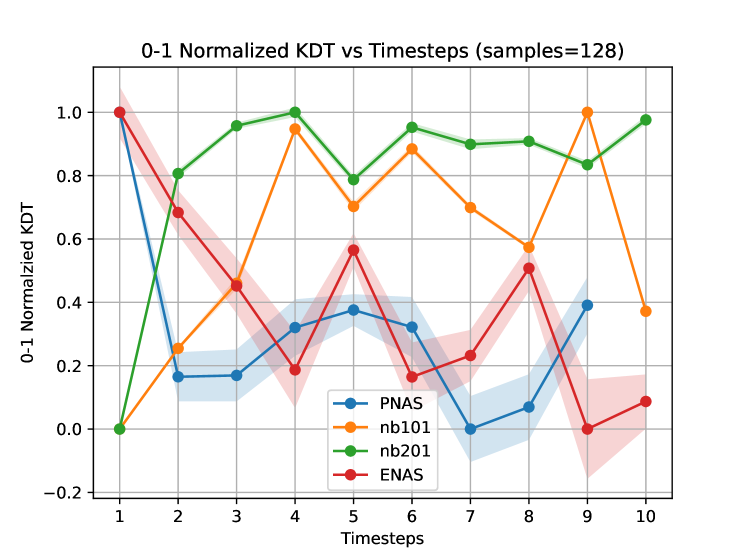
Figure 7: Testing the impact of time-steps in the training-analogous operation update regime. 0-1 normalized KDT for each space.

A.4.1 Neural Architecture Design Spaces

In this study, we examine various unique neural architecture design domains. We delve into NASBench-101 (Ying et al., 2019) and NASBench-201 (Dong & Yang, 2020), both of which are cell-based search spaces encompassing 423,624 and 15,625 architectures, respectively. While NASBench-101 is trained on CIFAR-10, NASBench-201 benefits from training on CIFAR-10, CIFAR-100, and ImageNet16-120. NASBench-301 (Zela et al., 2020) acts as a surrogate NAS benchmark with an impressive count of $10^{18}$ architectures. Meanwhile, TransNAS-Bench-101 (Duan et al., 2021) offers both a micro (cell-based) search area featuring 4096 architectures and a broader macro search domain with 3256 designs. For the scope of our study, we focus on the TransNASBench-101 Micro due to its cell-based nature. Each of these networks undergoes training across seven distinct tasks sourced from the Taskonomy dataset. The NASLib framework brings coherence to these search areas. NAS-Bench-Suite-Zero (Krishnakumar et al., 2022) expands the landscape by introducing two datasets from NAS-Bench-360 and four more from Taskonomy. It’s worth noting that the NDS dataset features ‘$FixWD$’ datasets, signifying that the architectures maintain consistent width and depth.

A.4.2 Training analogous predictor training

Given a DAG, the TA-GATESNing et al. (2022) encoding begins by obtaining the initial operation embedding for all operations based on their types. For $T$ time steps, an iterative process updates the operation embeddings, mimicking architecture parameter updates in training. Each step involves computing information flow via GCNs on the architecture DAG, and calling an MLP using the previous operation embedding; the output is then used in a backward GCN pass and then computing the operation embedding update. The last step concatenates the previous operation embedding with the forward and backward propagated information, feeds this to an MLP, and yields the updated operation embedding for the next step. The final architecture encoding uses the output of the $T$-th iterative refinement. In Figure 7 we study the impact of changing the number of time-steps on the over-all kendall tau correlation (KDT). The trend is inconsistent, and therefore we attempt to investigate the utility of the backward GCN.

Table 11: Sample Size 64 (left), 128 (right)

Space	DOpEmbUnrolled BMLP	Default		DOpEmbUnrolled GCN
PNAS	0.3244	0.3		0.3395
ENAS	0.409	0.3929		0.3764
nb201	0.7831	0.7795		0.7640
nb101	0.6055	0.6283		0.6041

DOpEmbUnrolled BMLP	Default		DOpEmbUnrolled GCN
0.4779	0.4684		0.4481
0.4925	0.4958		0.4498
0.7953	0.8007		0.7838
0.7122	0.7013		0.6993

To conduct a deeper investigation of this phenomenon, we study several aspects of training analogous predictor training. We look at BMLP, which is where we replace the backward ’GCN’ with a small MLP. Further, the backward GCN pass uses the output of the ’forward’ GCN along with the transposed adjacency matrix. This is then passed to an ’operation update MLP’ that takes as input BYI, which is the output of the backward GCN, BOpE, which is the operation embedding itself. In Table 15, Table 15, Table 15, Table 15 we can see that in all cases, BMLP outperforms having a backward GCN. Additionally, in many cases the BYI information does not add much value. However, it does not harm performance. Therefore, for further tests we will use BMLP with BYI,BOpE.

A.4.3 Inputs to backward MLP and gradient flow

From Figure 7, we have observed that 2 timesteps generally help but more timesteps are not useful for predictor performance. Additionally, we have replaced the entire backward GCN with a backward MLP. We now investigate which gradients need to be detached during iterative refinement. In the ’def’ (default) TA-GATES case, the BYI is not detached, whereas the BOpE is detached. In our tests, in ’all’, we detach BYI,BOpE and in ’none’, we do not detach any inputs to the BMLP. We find no clear pattern over 8 tests (3 trials each) in detach, except that it is better to either use the default rule or detach none of the gradients. For simplicity, we will detach none of the gradients. We again see that BYI is important for the BMLP, but the utility of BOpE is unclear. Further, In Table 10, we test whether we need to pass only the encoding at the output node of the forward GCN, or should we concatenate encodings at all nodes to pass to the backward MLP/GCN. Here, we find that there is no clear advantage of passing all node encodings and thus we only use the output node encoding.

A.4.4 Unrolled backward MLP computation

Here, we investigate different ways to unroll the backward computation to simplify the encoding process even further. In Table 11, we introduce two methods of unrolling the computation. We only unroll for 2 time-steps, which gives us a computational graph very similar to Figure 3. In the case of DOpEmbUnrolled BMLP, (Direct Op-Emb Unrolled to BMLP) we directly take the output of the forward GNN along with the operation embedding, pass it to an MLP and use that as the encoding for the next GNN. In the case of DOpEmbUnrolled GCN (Direct Op-Emb Unrolled to GCN) we directly take the output of the forward GNN along with the operation embedding and pass it to the backward-GCN instead of the BMLP, and use the output as an encoding for the next GNN. We find that unrolling the computation further improves predictive performance.

A.4.5 Final Predictor Architecture Design

Finally, this leads us to our own architecture design. In our architecture, we significantly simplify the predictor architecture. Firstly, we maintain a smaller GNN which refines the operation and hardware embedding. This refind embedding is passed to an MLP which maps the embedding back to the original dimensions. This refined embedding is passed directly to the larger GNN along with the adjacency matrix and node embeddings. We find that this simplified architecture performs better in most of our tests.

Table 12: ENAS Sample Size 64 (left), 128 (right). Ablation for backward pass. BMLP indicates that instead of replicating network, we do a simple 2 layer MLP for backward pass. BYI indicates whether we use the output of the forward pass network or not. BOpE indicates whether we use the output of the operation embedding itself or not. PM indicates that num params are approximately matched wrt TS $>$ 1. w / d indicates whether the matching happens by adjusting width or depth in forward gcn architecture. 2R implies that we simply use a small random perturb vector for operation update to ’regularize’ the network.

TS	BMLP	BYI	BOpE		KDT	Dev
2R	✗	✗	✗		0.3397	0.0018
1${}_{PM}^{d}$	✗	✗	✗		0.3832	0.0027
2	✓	✓	✗		0.3941	0.0061
3	✓	✗	✓		0.3973	0.0008
1${}_{PM}^{w}$	✗	✗	✗		0.3983	0.006
3	✓	✓	✗		0.3988	0.0054
2	✓	✗	✓		0.4142	0.0009

TS	BMLP	BYI	BOpE		KDT	Dev
2R	✗	✗	✗		0.4611	0.0010
1${}_{PM}^{w}$	✗	✗	✗		0.4635	0.0027
1${}_{PM}^{d}$	✗	✗	✗		0.4684	0.0007
2	✓	✗	✗		0.4686	0.0005
3	✗	✓	✗		0.4847	0.0007
3	✓	✗	✓		0.4888	0.0039
2	✓	✗	✓		0.4975	0.0021

Table 13: NB201 Sample Size 64 (left), 128 (right). Ablation for backward pass.

TS	BMLP	BYI	BOpE		KDT	Dev
1${}_{PM}^{d}$	✗	✗	✗		0.7472	0.0005
1${}_{PM}^{w}$	✗	✗	✗		0.7475	0.0005
2R	✗	✗	✗		0.7521	0.0002
3	✓	✗	✗		0.7835	0.0002
2	✓	✓	✓		0.7845	0.0001
3	✓	✗	✓		0.7856	0.0001
3	✓	✓	✓		0.7882	0.0003
2	✓	✗	✓		0.7894	0.0002

TS	BMLP	BYI	BOpE		KDT	Dev
1${}_{PM}^{w}$	✗	✗	✗		0.7682	0.0
2R	✗	✗	✗		0.7718	0.0001
1${}_{PM}^{d}$	✗	✗	✗		0.7765	0.0005
2	✓	✗	✓		0.7918	0.0003
2	✓	✓	✓		0.7927	0.0004
3	✓	✓	✓		0.7953	0.0005
2	✓	✓	✗		0.7956	0.0001
3	✓	✗	✓		0.7971	0.0004

Table 14: PNAS Sample Size 64 (left), 128 (right). Ablation for backward pass.

TS	BMLP	BYI	BOpE		KDT	Dev
1${}_{PM}^{d}$	✗	✗	✗		0.3387	0.008
2R	✗	✗	✗		0.3494	0.0165
1${}_{PM}^{w}$	✗	✗	✗		0.3635	0.011
2	✗	✓	✗		0.364	0.0145
2	✓	✗	✓		0.3641	0.0055
3	✗	✓	✗		0.378	0.0106
2	✓	✓	✗		0.382	0.0092
3	✓	✓	✗		0.3852	0.0104

TS	BMLP	BYI	BOpE		KDT	Dev
1${}_{PM}^{d}$	✗	✗	✗		0.4352	0.012
2R	✗	✗	✗		0.4507	0.0063
2	✓	✗	✗		0.4625	0.0035
2	✓	✓	✗		0.4684	0.0033
3	✓	✓	✗		0.4709	0.0041
1${}_{PM}^{w}$	✗	✗	✗		0.4779	0.003
3	✗	✓	✗		0.4841	0.0005
2	✗	✓	✗		0.4897	0.0006

Table 15: NB101 Sample Size 64 (left), 128 (right). Ablation for backward pass.

TS	BMLP	BYI	BOpE		KDT	Dev
1${}_{PM}^{d}$	✗	✗	✗		0.6211	0.0007
1${}_{PM}^{w}$	✗	✗	✗		0.6273	0.0003
2	✓	✗	✗		0.6346	0.0001
2R	✗	✗	✗		0.6421	0.0063
2	✓	✓	✗		0.6466	0.0008
2	✓	✗	✓		0.6502	0.0004
3	✓	✓	✗		0.6515	0.0006
2	✓	✓	✓		0.6537	0.0003

TS	BMLP	BYI	BOpE		KDT	Dev
1${}_{PM}^{w}$	✗	✗	✗		0.6591	0.0003
2R	✗	✗	✗		0.6886	0.0063
1${}_{PM}^{d}$	✗	✗	✗		0.7008	0.0001
2	✓	✓	✗		0.707	0.0004
2	✓	✓	✓		0.7075	0.0001
2	✓	✗	✗		0.7089	0.0002
2	✓	✗	✓		0.7194	0.0001
3	✓	✓	✗		0.7276	0.0002

Table 16: ENAS Sample Size 64 (left), 128 (right). Ablation for backward pass. BMLP is always True. BYI indicates whether we use the output of the forward pass network or not. BOpE indicates whether we use the output of the operation embedding itself or not. DM indicates detachment mode. 2 timesteps fixed.

BYI	BOpE	DM	KDT	STD
✓	✗	def	0.4012	0.0062
✓	✗	none	0.4042	0.0044
✗	✓	none	0.4058	0.0013
✓	✗	all	0.4074	0.0053
✗	✓	def	0.4142	0.0009

BYI	BOpE	DM	KDT	STD
✓	✓	none	0.4694	0.0025
✗	✗	none	0.4716	0.0005
✗	✓	all	0.4958	0.003
✗	✓	def	0.4975	0.0021
✗	✓	none	0.511	0.0018

Table 17: NB201 Sample Size 64 (left), 128 (right). Ablation for backward pass.

BYI	BOpE	DM	KDT	STD
✗	✓	def	0.7795	0.0001
✓	✗	none	0.7853	0.0002
✓	✓	def	0.7859	0.0003
✗	✓	none	0.7871	0.0002
✓	✓	none	0.7949	0.0004

BYI	BOpE	DM	KDT	STD
✓	✓	def	0.7875	0.0003
✓	✗	none	0.7888	0.0002
✓	✓	none	0.7936	0.0005
✗	✓	none	0.7944	0.0002
✗	✓	def	0.8007	0.0002

Table 18: PNAS Sample Size 64 (left), 128 (right). Ablation for backward pass.

BYI	BOpE	DM	KDT	STD
✓	✓	def	0.3184	0.0011
✓	✗	none	0.3304	0.0067
✓	✗	all	0.333	0.006
✓	✗	def	0.3459	0.0074
✓	✓	none	0.3538	0.0045

BYI	BOpE	DM	KDT	STD
✓	✗	none	0.4388	0.0037
✓	✗	def	0.456	0.0036
✗	✓	none	0.4675	0.0039
✗	✓	all	0.4684	0.0042
✗	✓	def	0.474	0.0042

Table 19: NB101 Sample Size 64 (left), 128 (right). Ablation for backward pass.

BYI	BOpE	DM	KDT	STD
✓	✓	none	0.6329	0.0006
✓	✓	all	0.6432	0.0014
✗	✓	none	0.6436	0.0013
✗	✗	all	0.6552	0.0
✓	✓	def	0.6588	0.0

BYI	BOpE	DM	KDT	STD
✗	✗	def	0.7139	0.0001
✓	✓	all	0.7177	0.0001
✗	✗	none	0.7206	0.0002
✓	✗	def	0.728	0.0
✓	✗	none	0.735	0.0

Hyperparameter	Value	Hyperparameter	Value
Learning Rate	0.001	Weight Decay	0.00001
Number of Epochs	150	Batch Size	16
Number of Transfer Epochs	40 NB201, 30 FBNet	Transfer Learning Rate	0.003 NB201, 0.001 FBNet
Graph Type	DGF+GAT ensemble	Op Embedding Dim	48
Node Embedding Dim	48	Hidden Dim	96
Op-HW GCN Dims	[128, 128]	Op-HW MLP Dims	[128]
GCN Dims	[128, 128, 128]	MLP Dims	[200, 200, 200]
Number of Trials	3	Loss Type	Pairwise Hinge Loss (Ning et al., 2022)

Table 20: Hyperparameters used in the experiments. We run Optuna hyper-parameter optimization for 80 iterations.

NASBench201 ND Train-Test Correlation Latency Correlation between Test and Train devices
	1080ti_1	1080ti_32	1080ti_256	silver_4114	silver_4210r	samsung_a50	pixel3	essential_ph_1	samsung_s7
titan_rtx_256	0.772	0.792	0.812	0.947	0.982	0.975	0.878	0.897	0.854
gold_6226	0.958	0.956	0.776	0.912	0.927	0.894	0.711	0.898	0.920
fpga	0.828	0.841	0.888	0.943	0.974	0.959	0.872	0.924	0.888
pixel2	0.807	0.817	0.777	0.873	0.894	0.874	0.761	0.856	0.832
raspi4	0.654	0.669	0.735	0.844	0.878	0.875	0.967	0.808	0.758
eyeriss	0.415	0.434	0.893	0.586	0.618	0.625	0.722	0.624	0.521

NASBench201 N1 Train-Test Correlation Latency Correlation between Test and Train devices
	e_tpu_edge_tpu_int8	eyeriss	m_gpu_sd_675_AD_612_int8	m_gpu_sd_855_AD_640_int8	pixel3
1080ti_1	0.167	0.415	0.594	0.551	0.591
titan_rtx_32	0.127	0.403	0.595	0.547	0.599
titanxp_1	0.163	0.405	0.594	0.551	0.589
2080ti_32	0.174	0.424	0.603	0.560	0.601
titan_rtx_1	0.113	0.362	0.554	0.504	0.547

NASBench201 N2 Train-Test Correlation Latency Correlation between Test and Train devices
	1080ti_1	1080ti_32	titanx_32	titanxp_1	titanxp_32
e_gpu_jetson_nano_fp16	0.514	0.509	0.517	0.510	0.513
e_tpu_edge_tpu_int8	0.167	0.172	0.171	0.163	0.170
m_dsp_sd_675_HG_685_int8	0.593	0.594	0.599	0.591	0.596
m_dsp_sd_855_HG_690_int8	0.587	0.583	0.592	0.585	0.589
pixel3	0.591	0.611	0.598	0.589	0.607

NASBench201 N3 Train-Test Correlation Latency Correlation between Test and Train devices
	d_gpu_gtx_1080ti_fp32	e_gpu_jetson_nano_fp16	eyeriss	m_dsp_sd_675_HG_685_int8	m_gpu_sd_855_AD_640_int8
1080ti_1	0.362	0.514	0.415	0.593	0.551
2080ti_1	0.356	0.512	0.405	0.586	0.538
titanxp_1	0.356	0.510	0.405	0.591	0.551
2080ti_32	0.371	0.519	0.424	0.598	0.560
titanxp_32	0.370	0.513	0.423	0.596	0.564

NASBench201 N4 Train-Test Correlation Latency Correlation between Test and Train devices
	d_cpu_i7_7820x_fp32	e_gpu_jetson_nano_fp32	e_tpu_edge_int8	eyeriss	m_cpuSD_855_kryo_485i8	m_dspSD_675_HG_685i8	m_dspSD_855_HG_690i8	m_gpuSD_675_AD_612i8	m_gpuSD_855_AD_640i8	pixel2
1080ti_1	0.360	0.739	0.167	0.415	0.645	0.593	0.587	0.594	0.551	0.807
2080ti_1	0.353	0.730	0.168	0.405	0.635	0.586	0.581	0.581	0.538	0.791
titan_rtx_1	0.313	0.703	0.113	0.362	0.600	0.547	0.541	0.554	0.504	0.775

NASBench201 NA Train-Test Correlation Latency Correlation between Test and Train devices
	titan_rtx_1	titan_rtx_32	titanxp_1	2080ti_1	titanx_1	1080ti_1	titanx_32	titanxp_32	2080ti_32	1080ti_32	gold_6226	samsung_s7	silver_4114	gold_6240	silver_4210r	samsung_a50	pixel2
eyeriss	0.362	0.403	0.405	0.405	0.409	0.415	0.418	0.423	0.424	0.434	0.503	0.521	0.586	0.609	0.618	0.625	0.609
d_gpu_gtx_1080ti_fp32	0.315	0.346	0.356	0.356	0.362	0.362	0.369	0.370	0.371	0.376	0.438	0.450	0.488	0.507	0.511	0.513	0.501
e_tpu_edge_tpu_int8	0.113	0.127	0.163	0.168	0.166	0.167	0.171	0.170	0.174	0.172	0.221	0.246	0.243	0.268	0.256	0.261	0.299

Table 21: NASBench-201 task train-test correlations. HG: Hexagon; AD: Adreno; m: Mobile; SD: Snapdragon; e: Embedded; i8: int8. Rows are test devices, Column headers are training devices.

FBNet FD Train-Test Correlation Latency Correlation between Test and Train devices
	1080ti_1	1080ti_32	1080ti_64	silver_4114	silver_4210r	samsung_a50	pixel3	essential_ph_1	samsung_s7
fpga	0.226	0.419	0.605	0.674	0.679	0.865	0.906	0.700	0.713
raspi4	0.256	0.524	0.719	0.641	0.649	0.841	0.957	0.660	0.678
eyeriss	0.247	0.527	0.757	0.624	0.633	0.864	0.976	0.678	0.690

FBNet F1 Train-Test Correlation Latency Correlation between Test and Train devices
	2080ti_1	essential_ph_1	silver_4114	titan_rtx_1	titan_rtx_32
eyeriss	0.238	0.678	0.624	0.249	0.442
fpga	0.206	0.700	0.674	0.217	0.350
raspi4	0.241	0.660	0.641	0.251	0.450
samsung_a50	0.310	0.646	0.686	0.317	0.429
samsung_s7	0.293	0.650	0.649	0.312	0.352

FBNet F2 Train-Test Correlation Latency Correlation between Test and Train devices
	essential_ph_1	gold_6226	gold_6240	pixel3	raspi4
1080ti_1	0.258	0.207	0.536	0.249	0.256
1080ti_32	0.338	0.241	0.459	0.555	0.524
2080ti_32	0.312	0.214	0.449	0.519	0.492
titan_rtx_1	0.268	0.184	0.536	0.253	0.251
titanxp_1	0.286	0.222	0.568	0.270	0.276

FBNet F3 Train-Test Correlation Latency Correlation between Test and Train devices
	essential_ph_1	pixel2	pixel3	raspi4	samsung_s7
1080ti_1	0.258	0.300	0.249	0.256	0.307
1080ti_32	0.338	0.409	0.555	0.524	0.372
2080ti_1	0.240	0.287	0.243	0.241	0.293
titan_rtx_1	0.268	0.296	0.253	0.251	0.312
titan_rtx_32	0.313	0.369	0.471	0.450	0.352

FBNet F4 Train-Test Correlation Latency Correlation between Test and Train devices
	1080ti_64	2080ti_1	eyeriss	gold_6226	gold_6240	raspi4	samsung_s7	silver_4210r	titan_rtx_1	titan_rtx_32
1080ti_1	0.439	0.944	0.247	0.207	0.536	0.256	0.307	0.653	0.948	0.846
pixel2	0.496	0.287	0.767	0.747	0.678	0.747	0.629	0.653	0.296	0.369
essential_ph_1	0.414	0.240	0.678	0.670	0.663	0.660	0.650	0.608	0.268	0.313

FBNet FA Train-Test Correlation Latency Correlation between Test and Train devices
	1080ti_1	1080ti_32	1080ti_64	2080ti_1	2080ti_32	2080ti_64	titan_rtx_1	titan_rtx_32	titan_rtx_64	titanx_1	titanx_32	titanx_64	titanxp_1	titanxp_32	titanxp_64
gold_6226	0.207	0.241	0.323	0.178	0.214	0.297	0.184	0.209	0.274	0.232	0.270	0.344	0.222	0.250	0.303
essential_ph_1	0.258	0.338	0.414	0.240	0.312	0.395	0.268	0.313	0.388	0.300	0.379	0.427	0.286	0.362	0.406
samsung_s7	0.307	0.372	0.421	0.293	0.349	0.406	0.312	0.352	0.404	0.347	0.402	0.435	0.337	0.388	0.416
pixel2	0.300	0.409	0.496	0.287	0.388	0.485	0.296	0.369	0.466	0.328	0.449	0.512	0.318	0.425	0.486

Table 22: FBNet task train-test correlations. Rows are test devices, Column headers are training devices.

Device	Type	NB201	FBNet
HELP & HW-NAS-Bench Lee et al. (2021b); Li et al. (2021)
1080ti_1	GPU	✓	✓
2080ti_1	GPU	✓	✓
1080ti_32	GPU	✓	✓
2080ti_32	GPU	✓	✓
1080ti_256	GPU	✓	✓
2080ti_256	GPU	✓	✓
titan_rtx_1	GPU	✓	✓
titanx_1	GPU	✓	✓
titanxp_1	GPU	✓	✓
titan_rtx_32	GPU	✓	✓
titanx_32	GPU	✓	✓
titanxp_32	GPU	✓	✓
titan_rtx_256	GPU	✓	✓
titanx_256	GPU	✓	✓
titanxp_256	GPU	✓	✓
gold_6240	CPU	✓	✓
silver_4114	CPU	✓	✓
silver_4210r	CPU	✓	✓
gold_6226	CPU	✓	✓
samsung_a50	mCPU	✓	✓
pixel3	mCPU	✓	✓
samsung_s7	mCPU	✓	✓
essential_ph_1	mCPU	✓	✓
pixel2	mCPU	✓	✓
fpga	FPGA	✓	✓
raspi4	eCPU	✓	✓
eyeriss	ASIC	✓	✓
Device	Type	NB201	FBNet
EAGLEDudziak et al. (2020)
core_i7_7820x_fp32	CPU	✓	✗
snapdragon_675_kryo_460_int8	mCPU	✓	✗
snapdragon_855_kryo_485_int8	mCPU	✓	✗
snapdragon_450_cortex_a53_int8	mCPU	✓	✗
edge_tpu_int8	eTPU	✓	✗
gtx_1080ti_fp32	GPU	✓	✗
jetson_nano_fp16	eGPU	✓	✗
jetson_nano_fp32	eGPU	✓	✗
snapdragon_855_adreno_640_int8	mGPU	✓	✗
snapdragon_450_adreno_506_int8	mGPU	✓	✗
snapdragon_675_adreno_612_int8	mGPU	✓	✗
snapdragon_675_hexagon_685_int8	mDSP	✓	✗
snapdragon_855_hexagon_690_int8	mDSP	✓	✗

Table 23: Devices used in our paper and their categories (type). Note that we are referring to latency measurements on the same device with different batch sizes as a new device as well, this is because in some cases, there is a low correlation between these measurements.

Task Index	Type	Devices
ND	Train	1080ti_1
		1080ti_32
		1080ti_256
		silver_4114
		silver_4210r
		samsung_a50
		pixel3
		essential_ph_1
		samsung_s7
	Test	titan_rtx_256
		gold_6226
		fpga
		pixel2
		raspi4
		eyeriss
N1	Train	embedded_tpu_edge_tpu_int8
		eyeriss
		mobile_gpu_snapdragon_675_adreno_612_int8
		mobile_gpu_snapdragon_855_adreno_640_int8
		pixel3
	Test	1080ti_1
		titan_rtx_32
		titanxp_1
		2080ti_32
		titan_rtx_1
N2	Train	1080ti_1
		1080ti_32
		titanx_32
		titanxp_1
		titanxp_32
	Test	embedded_gpu_jetson_nano_fp16
		embedded_tpu_edge_tpu_int8
		mobile_dsp_snapdragon_675_hexagon_685_int8
		mobile_dsp_snapdragon_855_hexagon_690_int8
		pixel3
N3	Train	desktop_gpu_gtx_1080ti_fp32
		embedded_gpu_jetson_nano_fp16
		eyeriss
		mobile_dsp_snapdragon_675_hexagon_685_int8
		mobile_gpu_snapdragon_855_adreno_640_int8
	Test	1080ti_1
		2080ti_1
		titanxp_1
		2080ti_32
		titanxp_32

Table 24: Hardware devices for NASBench-201

Task Index	Type	Devices
N4	Train	desktop_cpu_core_i7_7820x_fp32
		embedded_gpu_jetson_nano_fp32
		embedded_tpu_edge_tpu_int8
		eyeriss
		mobile_cpu_snapdragon_855_kryo_485_int8
		mobile_dsp_snapdragon_675_hexagon_685_int8
		mobile_dsp_snapdragon_855_hexagon_690_int8
		mobile_gpu_snapdragon_675_adreno_612_int8
		mobile_gpu_snapdragon_855_adreno_640_int8
		pixel2
	Test	1080ti_1
		2080ti_1
		titan_rtx_1
N2	Train	titan_rtx_1
		titan_rtx_32
		titanxp_1
		2080ti_1
		titanx_1
		1080ti_1
		titanx_32
		titanxp_32
		2080ti_32
		1080ti_32
		gold_6226
		samsung_s7
		silver_4114
		gold_6240
		silver_4210r
		samsung_a50
		pixel2
	Test	eyeriss
		desktop_gpu_gtx_1080ti_fp32
		embedded_tpu_edge_tpu_int8

Table 25: Hardware devices for NASBench-201

Table 26: Hardware devices for FBNet

Task Index	Type	Devices
FD	Train	1080ti_1
		1080ti_32
		1080ti_64
		silver_4114
		silver_4210r
		samsung_a50
		pixel3
		essential_ph_1
		samsung_s7
	Test	fpga
		raspi4
		eyeriss
F1	Train	2080ti_1
		essential_ph_1
		silver_4114
		titan_rtx_1
		titan_rtx_32
	Test	eyeriss
		fpga
		raspi4
		samsung_a50
		samsung_s7
F2	Train	essential_ph_1
		gold_6226
		gold_6240
		pixel3
		raspi4
	Test	1080ti_1
		1080ti_32
		2080ti_32
		titan_rtx_1
		titanxp_1
F3	Train	essential_ph_1
		pixel2
		pixel3
		raspi4
		samsung_s7
	Test	1080ti_1
		1080ti_32
		2080ti_1
		titan_rtx_1
		titan_rtx_32

Task Index	Type	Devices
F4	Train	1080ti_64
		2080ti_1
		eyeriss
		gold_6226
		gold_6240
		raspi4
		samsung_s7
		silver_4210r
		titan_rtx_1
		titan_rtx_32
	Test	1080ti_1
		pixel2
		essential_ph_1
FA	Train	1080ti_1
		1080ti_32
		1080ti_64
		2080ti_1
		2080ti_32
		2080ti_64
		titan_rtx_1
		titan_rtx_32
		titan_rtx_64
		titanx_1
		titanx_32
		titanx_64
		titanxp_1
		titanxp_32
		titanxp_64
	Test	gold_6226
		essential_ph_1
		samsung_s7
		pixel2

References

- Abdelfattah et al. (2021) Abdelfattah, M. S., Mehrotra, A., Dudziak, Ł., and Lane, N. D. Zero-cost proxies for lightweight nas. arXiv preprint arXiv:2101.08134, 2021.
- Akhauri & Abdelfattah (2023) Akhauri, Y. and Abdelfattah, M. S. Multi-predict: Few shot predictors for efficient neural architecture search, 2023.
- Benmeziane et al. (2021) Benmeziane, H., Maghraoui, K. E., Ouarnoughi, H., Niar, S., Wistuba, M., and Wang, N. A comprehensive survey on hardware-aware neural architecture search, 2021.
- (4) Cai, H., Zhu, L., and Han, S. Proxylessnas: Direct neural architecture search on target task and hardware. In International Conference on Learning Representations.
- Cai et al. (2020) Cai, H., Gan, C., Wang, T., Zhang, Z., and Han, S. Once for all: Train one network and specialize it for efficient deployment. In International Conference on Learning Representations, 2020. URL https://arxiv.org/pdf/1908.09791.pdf.
- Dong & Yang (2020) Dong, X. and Yang, Y. Nas-bench-201: Extending the scope of reproducible neural architecture search. In International Conference on Learning Representations (ICLR), 2020. URL https://openreview.net/forum?id=HJxyZkBKDr.
- Duan et al. (2021) Duan, Y., Chen, X., Xu, H., Chen, Z., Liang, X., Zhang, T., and Li, Z. Transnas-bench-101: Improving transferability and generalizability of cross-task neural architecture search. In Proceedings of the IEEE/CVF Conference on Computer Vision and Pattern Recognition, pp. 5251–5260, 2021.
- Dudziak et al. (2020) Dudziak, L., Chau, T., Abdelfattah, M., Lee, R., Kim, H., and Lane, N. Brp-nas: Prediction-based nas using gcns. volume 33, pp. 10480–10490, 2020.
- Elsken (2023) Elsken, T. Bosch gmbh. private communication., September 2023.
- Kernighan & Lin (1970) Kernighan, B. W. and Lin, S. An efficient heuristic procedure for partitioning graphs. The Bell System Technical Journal, 49(2):291–307, 1970. doi: 10.1002/j.1538-7305.1970.tb01770.x.
- Krishnakumar et al. (2022) Krishnakumar, A., White, C., Zela, A., Tu, R., Safari, M., and Hutter, F. Nas-bench-suite-zero: Accelerating research on zero cost proxies. In Thirty-sixth Conference on Neural Information Processing Systems Datasets and Benchmarks Track, 2022.
- Lahitani et al. (2016) Lahitani, A. R., Permanasari, A. E., and Setiawan, N. A. Cosine similarity to determine similarity measure: Study case in online essay assessment. In 2016 4th International Conference on Cyber and IT Service Management, pp. 1–6, 2016. doi: 10.1109/CITSM.2016.7577578.
- Lee et al. (2021a) Lee, H., Hyung, E., and Hwang, S. J. Rapid neural architecture search by learning to generate graphs from datasets. In International Conference on Learning Representations, 2021a.
- Lee et al. (2021b) Lee, H., Lee, S., Chong, S., and Hwang, S. J. Help: Hardware-adaptive efficient latency prediction for nas via meta-learning. In 35th Conference on Neural Information Processing Systems (NeurIPS) 2021. Conference on Neural Information Processing Systems (NeurIPS), 2021b.
- Li et al. (2021) Li, C., Yu, Z., Fu, Y., Zhang, Y., Zhao, Y., You, H., Yu, Q., Wang, Y., Hao, C., and Lin, Y. {HW}-{nas}-bench: Hardware-aware neural architecture search benchmark. In International Conference on Learning Representations, 2021. URL https://openreview.net/forum?id=_0kaDkv3dVf.
- Li & Talwalkar (2019) Li, L. and Talwalkar, A. Random search and reproducibility for neural architecture search. arXiv preprint arXiv:1902.07638, 2019.
- Lindauer & Hutter (2019) Lindauer, M. and Hutter, F. Best practices for scientific research on neural architecture search. arXiv preprint arXiv:1909.02453, 2019.
- MacQueen et al. (1967) MacQueen, J. et al. Some methods for classification and analysis of multivariate observations. In Proceedings of the fifth Berkeley symposium on mathematical statistics and probability, volume 1, pp. 281–297. Oakland, CA, USA, 1967.
- Ming Chen et al. (2020) Ming Chen, Z. W., Zengfeng Huang, B. D., and Li, Y. Simple and deep graph convolutional networks. 2020.
- Nair et al. (2022) Nair, S., Abbasi, S., Wong, A., and Shafiee, M. J. Maple-edge: A runtime latency predictor for edge devices. In 2022 IEEE/CVF Conference on Computer Vision and Pattern Recognition Workshops (CVPRW), pp. 3659–3667. IEEE, 2022.
- Ning et al. (2022) Ning, X., Zhou, Z., Zhao, J., Zhao, T., Deng, Y., Tang, C., Liang, S., Yang, H., and Wang, Y. TA-GATES: An encoding scheme for neural network architectures. In Oh, A. H., Agarwal, A., Belgrave, D., and Cho, K. (eds.), Advances in Neural Information Processing Systems, 2022. URL https://openreview.net/forum?id=74fJwNrBlPI.
- Ning et al. (2023) Ning, X., Zheng, Y., Zhou, Z., Zhao, T., Yang, H., and Wang, Y. A generic graph-based neural architecture encoding scheme with multifaceted information. IEEE Transactions on Pattern Analysis and Machine Intelligence, 45(7):7955–7969, 2023. doi: 10.1109/TPAMI.2022.3228604.
- Tan et al. (2019) Tan, M., Chen, B., Pang, R., Vasudevan, V., Sandler, M., Howard, A., and Le, Q. V. Mnasnet: Platform-aware neural architecture search for mobile. pp. 2820–2828, 2019.
- Veličković et al. (2018) Veličković, P., Cucurull, G., Casanova, A., Romero, A., Lio, P., and Bengio, Y. Graph attention networks. In International Conference on Learning Representations, 2018.
- Wang et al. (2020) Wang, H., Wu, Z., Liu, Z., Cai, H., Zhu, L., Gan, C., and Han, S. Hat: Hardware-aware transformers for efficient natural language processing. In Proceedings of the 58th Annual Meeting of the Association for Computational Linguistics, 2020.
- White et al. (2020) White, C., Neiswanger, W., Nolen, S., and Savani, Y. A study on encodings for neural architecture search. In Advances in Neural Information Processing Systems, 2020.
- Wu et al. (2019) Wu, B., Dai, X., Zhang, P., Wang, Y., Sun, F., Wu, Y., Tian, Y., Vajda, P., Jia, Y., and Keutzer, K. Fbnet: Hardware-aware efficient convnet design via differentiable neural architecture search. In Proceedings of the IEEE/CVF Conference on Computer Vision and Pattern Recognition, pp. 10734–10742, 2019.
- Xu et al. (2020) Xu, Y., Xie, L., Zhang, X., Chen, X., Shi, B., Tian, Q., and Xiong, H. Latency-aware differentiable neural architecture search. arXiv preprint arXiv:2001.06392, 2020.
- Yan et al. (2020) Yan, S., Zheng, Y., Ao, W., Zeng, X., and Zhang, M. Does unsupervised architecture representation learning help neural architecture search? In NeurIPS, 2020.
- Yan et al. (2021) Yan, S., Song, K., Liu, F., and Zhang, M. Cate: Computation-aware neural architecture encoding with transformers. In ICML, 2021.
- Yang et al. (2020) Yang, A., Esperança, P. M., and Carlucci, F. M. Nas evaluation is frustratingly hard. 2020.
- Ying et al. (2019) Ying, C., Klein, A., Christiansen, E., Real, E., Murphy, K., and Hutter, F. Nas-bench-101: Towards reproducible neural architecture search. In International Conference on Machine Learning, pp. 7105–7114. PMLR, 2019.
- Yu et al. (2020) Yu, J., Jin, P., Liu, H., Bender, G., Kindermans, P.-J., Tan, M., Huang, T., Song, X., Pang, R., and Le, Q. Bignas: Scaling up neural architecture search with big single-stage models. In European Conference on Computer Vision, pp. 702–717. Springer, 2020.
- Zela et al. (2020) Zela, A., Siems, J., Zimmer, L., Lukasik, J., Keuper, M., and Hutter, F. Surrogate nas benchmarks: Going beyond the limited search spaces of tabular nas benchmarks, 2020. URL https://arxiv.org/abs/2008.09777.