Nonperturbative cavity quantum electrodynamics: is the Jaynes-Cummings model still relevant?

In this tutorial review, we briefly discuss the role that the Jaynes-Cummings model occupies in present-day research in cavity quantum electrodynamics with a particular focus on the so-called ultrastrong coupling regime. We start by critically analyzing the various approximations required to distill such a simple model from standard quantum electrodynamics. We then discuss how many of those approximations can, and often have been broken in recent experiments. The consequence of these failures has been the need to abandon the Jaynes-Cummings model for more complex models. In this, the quantum Rabi model has the most prominent role and we will rapidly survey its rich and peculiar phenomenology. We conclude the paper by showing how the Jaynes-Cummings model still plays a crucial role even in non-perturbative light-matter coupling regimes.

1 Introduction

The Jaynes-Cummings model (JCM) is a pivotal theoretical object in quantum optics, describing the quintessential interaction between light and matter at the quantum level. It models the simplest quantum emitter, a two-level system (TLS), interacting with a single electromagnetic degree of freedom, a discrete mode of a photonic cavity. Their interaction is described by a Hamiltonian composed of two terms with transparent physical interpretation: the first describes the emitter transitioning between the ground and the excited state by the absorption of a photon, and the second, its Hermitic conjugate, describes its de-excitation caused by photon emission. This simplicity has made the JCM an outstanding pedagogical tool in quantum optics, and a fundamental framework for understanding and analyzing light-matter interactions in cavity quantum electrodynamics (CQED) systems. Since the Nobel-worth experiments of Haroche and Wineland [1, 2], which for the first time allowed to experimentally measure some of the most peculiar predictions of the JCM, the study of CQED has grown into one of the most active in physics, with impact in fields as different as quantum information [3, 4, 5], chemistry [6, 7, 8], photonics [9, 10], material engineering [11, 12, 13, 14, 15], and many others. As the boundary of knowledge was pushed forward, some of the underlying hypotheses that allowed to distilling of the Platonic simplicity of the JCM out of the complexity of an interacting light-matter system have been stretched or altogether broken. This led in turn to a vast theoretical effort to extend the JCM to understand and solve these shortcomings.

This tutorial review aims to give an overview of the physics of and beyond the JCM, exploring under which conditions different approximations break down, how the theory can be modified to accommodate those situations, and which novel phenomenology becomes observable.

2 The minimal description of a cavity QED system

2.1 Introducing the Jaynes-Cummings model

The JCM model describes the idealized system represented in Fig. 1: a TLS coupled to a single electromagnetic mode of a cavity. Its Hamiltonian reads

$$\hat{H}_{\rm JC}=\hbar\omega_{c}\hat{a}^{{\dagger}}\hat{a}+\frac{\hbar\omega_{eg}}{2}\hat{\sigma}_{z}+\hbar\Omega_{\rm R}\left(\hat{a}\hat{\sigma}_{+}+\hat{a}^{{\dagger}}\hat{\sigma}_{-}\right).$$ (1)

Here $\hat{\sigma}_{z}$ and $\hat{\sigma}_{-}=\hat{\sigma}_{+}^{{\dagger}}=\hat{\sigma}_{x}-i\hat{\sigma}_{y}$ are Pauli matrices, $\hat{a}$ is the annihilation operator of a cavity photon with frequency $\omega_{c}$, satisfying $[\hat{a},\hat{a}^{{\dagger}}]=1$, $\omega_{eg}$ is the frequency of an optically active transition, and $\Omega_{\rm R}$ is the so-called vacuum Rabi frequency, which quantifies the light-matter interaction strength.

The intuitive understanding of light-matter interactions provided by the JCM is based on the concepts of absorption and emission, spontaneous and stimulated, first introduced by Einstein through his A, B coefficients [16]. The interaction part of the JCM Hamiltonian in Eq. (1), proportional to the vacuum Rabi frequency $\Omega_{\text{R}}$, is of the flip-flop type and whenever a photon is destroyed the TLS is excited, and vice versa. As a consequence, the sum of photon number plus TLS excitation is a conserved quantity, which can be formalized by introducing the excitation number operator

$$\hat{N}=\hat{a}^{{\dagger}}\hat{a}+\frac{1}{2}\left[\hat{\sigma}_{z}+1\right],$$ (2)

that commutes with the JCM Hamiltonian $[\hat{N},\hat{H}_{\rm JC}]=0$. In the spirit of the Noether theorem, conservation laws are linked to symmetries. So the conservation of the excitation number is reflected in the continuous $U(1)$ symmetry of the JCM where $\hat{N}$ is the generator of the phase shift transformation

$$\begin{split}e^{i\theta\hat{N}}\hat{a}e^{-i\theta\hat{N}}=\hat{a}e^{i\theta},\quad e^{i\theta\hat{N}}\hat{\sigma}_{-}e^{-i\theta\hat{N}}=\hat{\sigma}_{-}e^{i\theta},\end{split}$$ (3)

that leaves the Hamiltonian in Eq. (1) invariant. The symmetry and the commutativity of $\hat{N}$ with $\hat{H}$ allow us to express the JCM Hamiltonian in Eq. (1) in block-diagonal form, where each block is characterized by the quantum number $n\in\mathbb{N}_{+}$. Since each $n\neq 0$ eigenvalue of $\hat{N}$ is doubly-degenerate, with eigenstates $|n,g\rangle\,,|n-1,e\rangle$, the JCM can be put in two-by-two block-diagonal form (one-by-one for the $n=0$ non-degenerate ground state $|0,g\rangle$)

$$\hat{H}^{0}_{JC} =-\frac{\hbar\omega_{eg}}{2},$$ (4)

$$\hat{H}^{n}_{JC} =\left[\begin{array}[]{cc}\hbar\omega_{c}n-\frac{\hbar\omega_{eg}}{2}&\hbar\Omega_{\text{R}}\sqrt{n}\\ \hbar\Omega_{\text{R}}\sqrt{n}&\hbar\omega_{c}(n-1)+\frac{\hbar\omega_{eg}}{2}\end{array}\right],$$ (7)

where for each $n>0$ the eigenvalues of the n${}^{\text{th}}$ block, $\omega_{n,\pm}$, describe dressed states with $n$ excitations. The saturation of the TLS makes the system nonlinear, leading to a $n$-dependent intra-doublet splitting which at resonance reads [17, 18]

$$\omega_{n,+}-\omega_{n,-}=2\Omega_{\rm R}\sqrt{n}.$$ (8)

Notice that when the vacuum Rabi frequency is larger than the bare excitation frequencies $\Omega_{\rm R}>\omega_{c},\omega_{eg}$ the lowest eigenenergy of the JCM becomes negative, replacing the ground state of the system and thus changing its equilibrium properties. This prediction gives us a hint regarding the potential interest in studying the regime in which the vacuum Rabi frequency is comparable to or larger than the bare cavity and TLS frequencies.

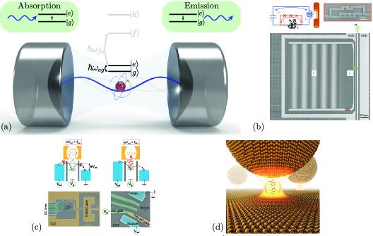
Figure 1: (a) Schematic illustration of the quantum light-matter interaction in a Fabry-Pérot cavity. A single atom is coupled to a single mode of the cavity field (blue wave). The figure shows the four assumptions that lead to the Quantum Rabi model. (i) A single atom is present in the cavity. (ii) Single-mode approximation, which assumes that only one cavity mode is relevant for the atom-field coupling. The other cavity modes are shaded. (iii) Dipolar approximation, with a constant electromagnetic field across the atom region. (iv) The two-level approximation, neglecting the higher-lying states shaded in the figure. The rotating wave approximation then leads to the Jaynes-Cumming model, whose two interaction terms are depicted on the top of the mirrors. These processes result in the coherent exchange of energy between the atom and the field. (b) A superconducting circuit that reaches the USC regime, taken from Ref. [19]. (c) Quantum dot coupled to a THz cavity in the USC regime, taken from Ref. [20]. (d) Plasmonic nanocavity device, taken from Ref. [21].

2.2 Why we need to go beyond the JCM: three experimental examples

The JCM is usually employed to describe systems in the strong coupling regime of CQED [22], in which the vacuum Rabi frequency becomes larger than the loss rates for the light ($\gamma$ ) and matter ($\kappa$) degrees of freedom, and we can resolve the resonant $n=1$ splitting $\omega_{1,+}-\omega_{1,-}=2\Omega_{\mathrm{R}}$ as from Eq.8. It is thus useful to introduce the cooperativity parameter $C=4\Omega_{\rm R}^{2}/(\gamma\kappa)$[18], with $C>1$ marking the onset of the strong coupling regime.

When the coupling becomes instead comparable to the frequencies of the bare excitations, the system enters a different regime characterized by a novel non-perturbative phenomenology. Such a regime has been named ultrastrong coupling (USC) regime [23, 24, 25]. By analogy with the cooperativity, it is useful to introduce the normalized coupling parameter $\zeta=4\Omega_{\rm R}^{2}/(\omega_{c}\omega_{eg})$, with $\zeta\sim O(1)$ identifying the USC regime [26] (the value $\zeta=0.04$, corresponding in the resonant case to $\Omega_{\rm R}=0.1\omega_{c}$, is usually used as threshold but this is only a historical accident [27]).

In the state-of-the-art experiments with Rydberg atoms in high-finesse optical cavities $C\sim 10-100\gg 1$ , but at the same time $\zeta\sim 10^{-5}\ll 1$ [18]. It was indeed shown in [28] that for a single hydrogenoid atom coupled to a resonant electric field, the normalized coupling can be written as $\Omega_{\text{R}}/\omega_{c}\approx\alpha_{\rm fs}^{3/2}/(\ell\pi\sqrt{V})$, where $\alpha_{\rm fs}\approx 1/137$ is the fine structure constant, $\ell$ is the principal quantum number, and $V$ the cavity volume expressed in units of a cube with half-wavelength sides. Without extreme subwavelength confinement, which is often accompanied by large losses [29], it is thus impossible to achieve non-perturbative light-matter USC on a single atom due to the fundamental hard bound imposed by the fine structure constant. From this analysis, it seems that the single particle USC regime is forbidden by the very basic principles of QED.

To circumvent this bound one can only rely on artificial, highly engineered systems where the dynamics of the electromagnetic field is mediated by a material component [28]. In particular, considering superconducting circuits it was found that the fine structure constant is rescaled by the circuit impedance $\alpha_{\rm fs}\longmapsto\left(Z/Z_{0}\right)^{\ell}\alpha_{\rm fs}$, where $Z_{0}=1/(\epsilon_{0}c)$ is the vacuum impedance, while $\ell=\pm 1$ dependently from the origin of the coupling (capacitive, inductive,etc…)[30, 31]. Beyond superconducting circuits only, this concept has a more broad application and similar scaling can be found also for plasmonic cavities, metamaterials and in general for any sub-wavelength resonant structure [32, 33]. In such setups the impedance has no bound in principle (if not merely technological), and a fully non-perturbative USC is possible, with values of $\zeta\sim 0.01-100$.

In Table 1 we report three examples of CQED setups working in various frequency regimes where a TLS coupled to a photonic resonator reaches the USC regime.

System	Cavity $\omega_{c}$	Atom $\omega_{eg}$	Coupling $\Omega_{\rm R}$	$\zeta$
Superconducting circuits [19]	35.2 GHz	23.9 GHz	35.2 GHz	6
Molecular plasmonic cavities [21]	452 THz	452 THz	73 THz	0.03
Graphene quantum dots [20]	25 THz	3.8 THz	49 THz	101

Table 1: Parameters of CQED setups in which a TLS coupled to a photonic resonator reaches the USC regime.

Note that the performance of the molecular plasmonic setup [21] was just close to USC physics. It was nevertheless shown how small modifications [34] could increase the coupling even further. In Fig. 1 we shows these three setups: superconducting circuits (b) [19] (also in their multimode or multi-qubit USC versions [35, 36, 37, 38, 39]), carbon nanotube quantum dots in THz cavities (c) [20], and molecules in plasmonic resonators (d) [21, 40, 34, 41]. Notwithstanding their differences, these USC systems share the same underlying CQED structure: a discrete electronic transition interacts coherently with a confined electromagnetic field. Still, the JCM does not correctly reproduce their features.

3 Understanding the Jaynes-Cummings model from QED

In order to understand this failure, and obtain a new model applicable in the USC regime and which recovers the JCM for weaker coupling strengths, we need first to understand how the JCM itself is obtained. Its clear depiction of light-matter interactions can be rigorously derived via a series of approximations from the non-relativistic quantum electrodynamics (QED) Hamiltonian. We list here the main steps to distill the JCM from the underlying QED theory, with the main approximations schematically represented in Fig. 1.

3.1 Dipolar approximation

To start, the JCM considers the light-matter interaction in the dipolar approximation. Formally this is obtained by expressing the full non-relativistic QED Hamiltonian in the so-called Poincaré gauge [42]: truncating its multipolar expansion to the lowest order, one obtains the dipole gauge Hamiltonian [43]. In simpler terms, when the electromagnetic field does not vary too much on the length scales of the TLS spatial extension, it can be considered spatially uniform. As a consequence, the light-matter interaction Hamiltonian can be derived by considering the energy of a dipole $\hat{\mathbf{d}}$ in a uniform electric field $\hat{\mathbf{E}}$

$$\hat{H}_{I}\propto\hat{\mathbf{d}}\cdot\hat{\mathbf{E}}.$$ (9)

This is a safe approximation for atoms in microwave cavities [1], but much less so for extended objects like molecules or quantum dots [44, 45, 46], or in nanophotonic resonators in which higher-order modes can be excited [47] and can lead to the phenomenon of fluorescence quenching [48]. In general, the presence of selection rules can suppress the dipole coupling in favor of other type of multipolar interactions due to symmetry [44, 49, 50].

3.2 Modelling the emitter as a TLS

While transitions in spin doublets can be exactly modeled as TLS, most quantum emitters are implemented with electronic transitions. The number of trapped electronic states can be substantially larger than two, and the possibility of focusing only on a single, discrete transition, between the ground state ($|g\rangle$) and a single excited state ($|e\rangle$) rests on the assumption that the coupling with all the other parts of the spectrum can be neglected. The evolution of the system can thus be considered to span only the two-dimensional Hilbert space $\left[\ket{g},\ket{e}\right]$. Using the Pauli matrices we can then describe any operator in the two-level subspace, for instance, the atomic dipole operator becomes

$$\hat{\mathbf{d}}\propto|e\rangle\langle g|+|g\rangle\langle e|=\hat{\sigma}_{-}+\hat{\sigma}_{+}.$$ (10)

The reason to ignore the other energy levels is that they are out-of-resonance, a justification so pervasive in physics that its assumptions are sometimes overlooked and can become surprisingly fragile in state-of-the-art CQED setups [51]. When this approximation breaks down modifications of the electronic wavefunction can be obtained. The coupled wavefunctions are interference patterns of the bare ones, and thus very sensitive and tunable [52, 53, 54, 55], a phenomenology referred to as very strong coupling.

3.3 Considering a single cavity mode

Analogously to the matter degrees of freedom, the photonic resonator also hosts a complete set of modes [56], both discrete and belonging to a continuum. If the field is strongly confined in a cavity or in any artificial structure (e.g. subwavelength resonators), the energy spacing between the different electromagnetic modes is such that we can discard all of them except the one that is most resonant with the optically active transition of interest. In such a way the cavity dynamics is completely described as a harmonic oscillator, with annihilation operator $\hat{a}$, and the electric field operator is given by

$$\hat{\mathbf{E}}\propto\hat{a}+\hat{a}^{{\dagger}}.$$ (11)

When this approximation is violated and the light-matter coupling becomes larger than the free spectral range we reach a different regime which has been called superstrong coupling [57]. In such a regime considering a single photonic mode allows faster-than-light signalling [58].

Analogously to the electronic case in the very strong coupling regime, the electromagnetic field of the coupled modes in the superstrong coupling regime are linear superpositions of multiple uncoupled electromagnetic modes, and dynamical modifications of subwavelength mode profile can be achieved [59, 60]. The coupling of different electromagnetic modes also provides extra degrees of freedom to the wavefunctions of the coupled light-matter eigenmodes, which at larger values of the normalized coupling can bend to avoid the dipoles. This also realizes one among the various mechanisms that leads to the phenomenon of light-matter decoupling [61] described in Sec. 8.

3.4 Applying the rotating wave approximation

The rotating wave approximation (RWA) is ubiquitous in physics even if known with different names, another one being secular approximation from its use in celestial mechanics, where the errors introduced would have become observable only over centuries. In the context of CQED is implemented by the following reduction

$$\hat{\mathbf{d}}\cdot\hat{\mathbf{E}}\propto\left(\hat{\sigma}_{-}+\hat{\sigma}_{+}\right)\left(\hat{a}+\hat{a}^{{\dagger}}\right)\approx\,\hat{\sigma}_{-}\hat{a}^{{\dagger}}+\hat{\sigma}_{+}\hat{a}.$$ (12)

This approximation is the crucial one in defining the light-matter interactions in terms of absorption/emission processes, as it consists in neglecting terms which lack an intuitive physical understanding and whose impact becomes non-negligible only in the USC regime.

Given the importance of this approximation for the definition of the ultrastrong coupling regime a more in-depth discussion of the consequences of going beyond the rotating-wave-approximation will be given in the next section (Sec. 4).

4 Unwind the rotating-wave: the Rabi model

For large enough values of the light-matter coupling strength all these approximation but the dipole one eventually break down [32, 25]. In the region of interest for current experiments, the RWA is the first one to be broken and hence the first we discuss here.

4.1 Re-introducing the counter-rotating terms

The JCM without the RWA it the so-called quantum Rabi model (QRM), described by the Hamiltonian

$$\hat{H}_{\rm R}=\hbar\omega_{c}\hat{a}^{{\dagger}}\hat{a}+\frac{\hbar\omega_{eg}}{2}\hat{\sigma}_{z}+\hbar\Omega_{\rm R}(\hat{a}+\hat{a}^{{\dagger}})\hat{\sigma}_{x}.$$ (13)

Since $\hat{\sigma}_{x}=\hat{\sigma}_{-}+\hat{\sigma}_{+}$, the interaction of the Rabi Hamiltonian contains terms proportional to $\hat{a}^{{\dagger}}\hat{\sigma}_{+}$ and $\hat{a}\hat{\sigma}_{-}$. These terms are not of the flip-flop type, as they involve the simultaneous creation (destruction) of a photon and an atomic excitation, breaking the intuition based on the absorption/emission paradigm. They are called counter-rotating because switching to the interaction picture Hamiltonian they evolve as $\hat{a}\hat{\sigma}_{-}e^{-i(\omega_{c}+\omega_{eg})t}$, contrary to the flip-flop terms evolving as $\hat{a}\hat{\sigma}_{+}e^{-i(\omega_{c}-\omega_{eg})t}$ [42]. At resonance $\omega_{c}=\omega_{eg}$, the flip-flop terms become time-independent, while the counter rotating terms keep oscillating with frequency $2\omega_{c}$ [42]. These terms thus couple states with different energies, and their impact scales in perturbation theory with powers of the coupling $\Omega_{\mathrm{R}}$ divided the bare frequencies $\omega_{c}$ and $\omega_{eg}$, becoming non-negligible only in the USC regime.

4.2 The validity of the RWA and the boundary of the USC regime

In Sec. 2 we have seen that the JCM has an internal $U(1)$ symmetry that reduces its Hamiltonian in a block diagonal form composed by a scalar and infinite two-by-two blocks, allowing for a simple analytical solution. On the contrary the Rabi model does not have this symmetry: the counter-rotating terms do not commute with the excitation number operator $[\hat{N},\hat{a}^{{\dagger}}\hat{\sigma}_{+}]\neq 0$, $[\hat{N},\hat{a}\hat{\sigma}_{-}]\neq 0$. Counter-rotating terms, adding or subtracting pairs of excitations, couple only states with even or odd excitation numbers. The system thus still possesses a $\mathbb{Z}_{2}$ symmetry, given by the invariance under parity transformation $\hat{a}\mapsto-\hat{a}$, $\hat{\sigma}_{-}\mapsto-\hat{\sigma}_{-}$. The simple analytical solution of the JCM is not available anymore, even though an exact analytical solution can still be obtained by exploiting the remaining symmetry [62]. The structure of the solution is however more intricated and the intuition developed in the JCM is lost [63, 64, 65, 66]. In any case, the Rabi model can be easily diagonalized numerically, for instance using the QuTip python library [67].

The transition from JCM to Rabi model is not sharp, but rather a crossover, where the spectrum of the Rabi model is indistinguishable from the JCM spectrum when the light-matter coupling is sufficiently small $\Omega_{\rm R}\ll\omega_{c},\omega_{eg}$, as visible in the left-side of Fig. 2(a). By further increasing the light-matter coupling the difference between the Rabi model and the JCM becomes more prominent due to the increasing importance of the counter-rotating terms. As pointed out in Ref. [26], their relevance can be evaluated by means of perturbation theory by computing the matrix element of the operators $\Omega_{\rm R}\hat{a}\hat{\sigma}_{-}$ between different $n,n^{\prime}$ excitation blocks. For instance, taking the simplest case of $n,n^{\prime}=n+1$, the RWA can be applied only if $\Omega_{\rm R}^{2}|\langle{n,g|\hat{a}\hat{\sigma}_{-}|n+1,e\rangle}|^{2}/(\omega_{c}+\omega_{eg})^{2}\ll 1$. The RWA regime of validity, delimited by the upper bound of this equation, namely

$$n_{\mathrm{max}}=\frac{(\omega_{c}+\omega_{eg})^{2}}{\Omega_{\rm R}^{2}},$$ (14)

is shaded in blue in Fig. 2(a). From here is clear that the JCM is a low-coupling and low-energy effective model of the Rabi one. Reaching the boundary of validity of the RWA has also well visible observable physical consequences. The most striking one is probably the Bloch-Siegert shift, which was first measured in superconducting circuits [68] from the transmission spectroscopy, and successively confirmed also in other different CQED platforms such as Landau polariton setups [69]. Let’s note that the breaking of the RWA is the original definition of the USC [70], and it was used for its first experimental validation [27].

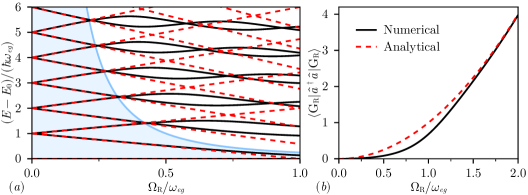
Figure 2: (a) Energy spectrum of the resonant Rabi model (black solid lines) and JCM (red dashed lines) as a function of the coupling strength. The region of validity of the RWA is highlighted in cyan, whose boundary is given by the cyan solid line. (b) The plot of the number of photons in the ground state of the quantum Rabi model by numerical diagonalization (black solid line) and using the first order term from Eq. 15 (red dashed line).

4.3 The non-empty vacuum beyond RWA

One of the most striking and investigated consequences of the presence of counter-rotating terms is that the empty cavity vacuum (i.e., the JCM ground state $|{\rm G}_{\rm JC}\rangle=|0,g\rangle$) is not anymore an eigenstate of the system. In fact, in the Rabi model, the ground state coincides with the empty cavity vacuum only for vanishing light-matter coupling and is then progressively filled by photons as the light-matter coupling increases. Using the same perturbative approach as in the previous section, one can compute the ground state virtual photon population, obtaining

$$\langle{{\rm G}_{\rm R}|\hat{a}^{{\dagger}}\hat{a}|{\rm G}_{\rm R}\rangle}\propto\left(\frac{\Omega_{\rm R}}{\omega_{c}}\right)^{2}+O\left[\left(\frac{\Omega_{\rm R}}{\omega_{c}}\right)^{4}\right].$$ (15)

This result is not specific to the Rabi model only, but rather a generic feature of USC systems. For instance in Fig. 2(b) we see the vacuum photon expectation number computed in the quantum Rabi model. The JCM would instead result in a photon population strictly vanishing in the ground state.

The presence of these photons in the coupled ground state (often referred to as virtual photons) is a typical non-perturbative phenomenon reminiscent, mutatis mutandis, of the quark-gluon gas populating the non-empty vacuum of quantum chromodynamics (QCD) [71]. The possibility of detecting these virtual photons was a central interest in the initial development of the theory of the USC regime [70], where CQED systems were identified as ideal playgrounds to study the fascinating and still mysterious physics of vacuum phenomena in QED [72].

As it will be explained in more detail in the next Sec. 7 observing quantum vacuum physics is not an easy task, because virtual photons (and virtual particles in general) are normally directly unobservable in experiments and the only proposal in this direction has been to measure the static charge displacement caused by virtual electronic excitations in an asymmetric system [73]. Otherwise, the observation of virtual photons is usually studied under a time-dependent perturbation [74] or electrical current [75] providing the required energy to convert virtual photons to real ones, or weakly coupling the system to another external probe system and observing its modified emission properties [76, 77, 78].

4.4 Excited states beyond RWA: multi-photon non-linear processes

The action of the counter-rotating terms in the USC regime impacts also the qualitative nature of the excitation spectrum. In particular, breaking the conservation of the excitation number allows non-linear processes with the absorption-emission of multiple photons at the same time [79]. This phenomenology is even richer when we explicitly break also the remaining $\mathbb{Z}_{2}$ symmetry, for instance considering the co-called asymmetric Rabi model

$$\hat{H}_{\rm aR}=\omega_{c}\hat{a}^{{\dagger}}\hat{a}+\frac{\omega_{eg}}{2}\hat{\sigma}_{z}+\Omega_{\rm R}(\hat{a}+\hat{a}^{{\dagger}})\hat{\sigma}_{x}+\frac{\epsilon}{2}\hat{\sigma}_{x}.$$ (16)

Here $\epsilon$ quantifies the explicit symmetry breaking and can be interpreted as an external static electric or magnetic field, as commonly employed in circuit QED [19, 80].

Increasing the value of $\epsilon$ opens some non-trivial avoided crossings in the spectrum, allowing the system to undergo multi-photon Rabi oscillations that might be used for the generation of multi-photons Fock states [81, 79, 82]. Here a single atom can emit simultaneously multiple photons with a single transition due to the USC. Differently from multi-photon processes arising in devices with non-linear quadrupolar light-matter coupling [83, 49], this dynamics is a USC consequence of the interplay between the linear dipole coupling and the non-linearity (or saturability) of the TLS. These effects are typically called tunneling resonances [84] since their mathematical description is identical to tunneling resonances appearing in the physics of electronic transport assisted by phonons through molecular or nanostructure quantum dots [85, 86, 87, 88]. They are currently a major reason for interest in the development of these platforms projecting also interesting new technological perspectives on the USC regime [89, 90, 91, 37, 36].

5 Gauging effective models

When building a theoretical model of a quantum system, it is often useful to consider only a limited subspace of its full Hilbert space (generally the lowest-energy states). In the case of light-matter coupled systems, this projection could introduce the risk of compromising the gauge invariance [92, 93, 51, 94, 95, 96, 97, 98]. Gauge invariance is a fundamental property of QED, ensuring that the dynamics remain unaltered upon gauge transformations. Truncating the Hilbert space can nevertheless break this fundamental symmetry, leading to physical results that depend on the (unphysical) choice of the gauge used to describe the electromagnetic field.

To better understand the problem, let’s consider the two most used gauges to study non-relativistic light-matter interactions: the Coulomb and the Power-Zienau-Woolley gauges [99, 42], where the latter is also known as multipolar or dipole gauge. Both gauges are also dubbed in the literature as the $\hat{\mathbf{p}}\cdot\hat{\mathbf{A}}$ or velocity gauge and the $\hat{\mathbf{d}}\cdot\hat{\mathbf{E}}$ or length gauge, where $\hat{\mathbf{p}}$ and $\hat{\mathbf{d}}=q\hat{\mathbf{x}}$ are the particle momentum and electric dipole moment with charge $q$ and displacement $\hat{\mathbf{x}}$. $\hat{\mathbf{A}}$ and $\hat{\mathbf{E}}$ are the vector potential and the electric field. If we consider the transition matrix elements between two states $|j\rangle$ and $|k\rangle$ of a particle with mass $m$, position $\hat{\mathbf{x}}$, and momentum $\hat{\mathbf{p}}$ we can easily derive the equation [100]

$$\langle j|\hat{\mathbf{p}}|k\rangle=im\omega_{jk}\langle j|\hat{\mathbf{x}}|k\rangle.$$ (17)

This relation shows that the matrix elements of the momentum are proportional to those of the position, with a proportionality factor linear in the energy difference between the two states $\omega_{jk}$. In the Coulomb gauge, where the interaction Hamiltonian is of the form $\hat{\mathbf{p}}\cdot\hat{\mathbf{A}}$, the matrix element thus vanishes more slowly with the detuning than in the $\hat{\mathbf{d}}\cdot\hat{\mathbf{E}}$ case, making the approximation of modeling the matter system as a TLS, ignoring out-of-resonance states, more fragile.

To obtain a quantitative understanding of how serious this problem of gauge non-invariance can be, we can start from the Hamiltonian describing a one-dimensional particle interacting with a single photonic mode in the Coulomb gauge $\nabla\cdot\hat{\mathbf{A}}=0$ (for major details on its derivation see, e.g., Refs. [99, 42, 32])

$$\hat{\mathcal{H}}_{\mathrm{C}}=\frac{1}{2m}\left(\hat{{p}}-q\hat{{A}}\right)^{2}+V(\hat{{x}})+\hbar\omega_{c}\hat{a}^{\dagger}\hat{a}\,.$$ (18)

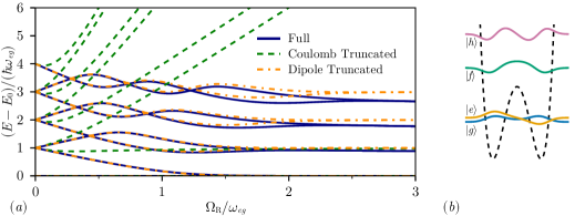
Figure 3: (a) Comparison of the lowest eigenvalues with respect to the ground state energy $E_{0}$ as a function of the coupling strength $\Omega_{\mathrm{R}}$, for the two truncated Hamiltonians in the Coulomb ($\hat{H}_{C}$, green dashed) and dipole ($\hat{H}_{D}$, orange dash-dotted) gauges. They are compared to the full Hamiltonian $\hat{\mathcal{H}}_{\mathrm{C}}$ in Eq. 18. The Coulomb gauge already deviates at very small values of $\Omega_{\mathrm{R}}$. In contrast, the dipole gauge breaks down at much higher values. (b) First four eigenstates of the atom Hamiltonian, with the same parameters used in panel (a). The double-well potential is modeled as $V(x)=Ax^{4}-Bx^{2}$, and the used parameters are $m=1$, $A=50$, and the anharmonicity $mB^{3}/(\hbar^{2}A^{2})=45$.

The Hamiltonian in the dipole gauge can be obtained by performing a gauge transformation [44, 99, 42], which is implemented in quantum mechanics by the unitary transformation: $\hat{\mathcal{H}}_{\mathrm{D}}=\hat{\mathcal{U}}\hat{\mathcal{H}}_{\mathrm{C}}\hat{\mathcal{U}}^{{\dagger}}$, with $\hat{\mathcal{U}}={\exp}[\frac{q}{\hbar}{A}_{0}\hat{{x}}\left(\hat{a}-\hat{a}^{\dagger}\right)]$, and $A_{0}$ the zero point fluctuation of the vector potential. The two Hamiltonians $\hat{\mathcal{H}}_{\mathrm{C}}$ and $\hat{\mathcal{H}}_{\mathrm{D}}$ have the same spectrum, being related by a unitary transformation. Projecting them onto the two lowest-energy states $\ket{g}$ and $\ket{e}$ of the uncoupled matter system, through the projection operator $\hat{P}=\outerproduct{g}{g}+\outerproduct{e}{e}$, we obtain the Hamiltonians describing the interaction of a single-mode electromagnetic field with a two-level system: $\hat{H}_{\mathrm{C}}=\hat{P}\hat{\mathcal{H}}_{\mathrm{C}}\hat{P}$ in the Coulomb gauge, and $\hat{H}_{\mathrm{D}}=\hat{P}\hat{\mathcal{H}}_{\mathrm{D}}\hat{P}$ in the dipole gauge.

In Fig. 3(a) we compare the eigenvalues of the full Hamiltonian in Eq. 18 with those of the of two projected Hamiltonians $\hat{H}_{\mathrm{C}}$ and $\hat{H}_{\mathrm{D}}$ as a function of the vacuum Rabi frequency $\Omega_{\mathrm{R}}\equiv q\omega_{c}A_{0}\langle e|\hat{x}|g\rangle/\hbar$. We consider a quartic potential in which the energy separation between the first two modes is 12 times smaller than the gap between the second and the third. As the coupling increases, deviations between the three models occur, already at the onset of the USC regime in the Coulomb gauge and for much larger values of the coupling in the dipole gauge. However, increasing the atom’s anharmonicity extends the range of agreement of the dipole gauge with the untruncated case. It is worth noticing that the gauge choice that reduces the error on the truncated Hilbert space is system dependent [94, 101, 102, 98].

Gauge invariance can be also implemented already in the two-level subspace by performing the minimal coupling replacement directly in the truncated subspace, that is applying the following unitary transformation to the free photon Hamiltonian only  [95, 96]

$$\hat{U}={\exp}\left[\frac{q}{\hbar}A_{0}\hat{P}\hat{x}\hat{P}\left(\hat{a}-\hat{a}^{\dagger}\right)\right]={\exp}\left[\frac{\Omega_{\mathrm{R}}}{\omega_{c}}\hat{\sigma}_{x}\left(\hat{a}-\hat{a}^{\dagger}\right)\right].$$ (19)

The same results can have also been obtained following a lattice gauge theory approach [103].

6 Single particle vs collective coupling

Aside from the modification of the photonic vacuum, the USC is predicted to modify also the state and properties of the matter counterpart, represented in the JCM or Rabi model by a TLS [104, 63, 105, 84]. From this observation, a strong interest has arisen to modify and control the properties of electrons, molecules, or devices exploiting the quantum fluctuations of the USC vacuum [14, 106]. For instance, the USC between a single electron and the resonator has been shown to have a strong impact on electron transport [20], thus becoming very interesting for more involved device operations with application purposes [107, 108]. Generalizing this concept to any light-matter systems is certainly appealing as a powerful technological framework, but also as a new way to explore the fundamental science behind the quantum vacuum [72].

6.1 Bosonising the light-matter interactions

Solid-state CQED setups, especially those in which USC has been achieved, are usually not well described by the JCM nor by the Rabi model because of the presence of multiple dipoles participating in the light-matter dynamics. A minimal description is provided by generalizing the JCM or the Rabi model where multiple TLSs are identically coupled to the same photonic mode (which means their separation is much smaller than the wavelength), giving the so-called Dicke model [109]

$$\hat{H}_{I}\propto\Omega_{\rm R}(\hat{a}+\hat{a}^{{\dagger}})\sum_{i=1}^{N}\hat{\sigma}_{x}^{i}\approx\sqrt{N}\Omega_{\rm R}(\hat{a}+\hat{a}^{{\dagger}})(\hat{b}+\hat{b}^{{\dagger}}).$$ (20)

Here the index $i$ on the Pauli matrices addresses the different TLSs. We introduced the collective annihilation operator $\hat{b}=\sum_{i=1}^{N}\hat{\sigma}_{-}^{i}/\sqrt{N}$, describing a collective excitation of all the TLSs. This operator satisfies $[\hat{b},\hat{b}^{{\dagger}}]\approx 1+O(\frac{n_{x}}{N})$ in the dilute regime, that is when the number of excitations $n_{x}$ is much smaller than the total number $N$ of TLSs [110, 111].

This transformation also leads to a vacuum Rabi frequency enhanced by a factor $\sqrt{N}$, often referred as collective enhancement, which makes it much simpler to reach extreme values of the coupling [70, 27, 112, 113]. Increasing the number of dipoles the coupling increases but the optical nonlinearity decreases. The saturation of the TLS washes out, as the system is able to absorb multiple photons. The system becomes then well described by a linear optical approach, where both the cavity and the material are described by harmonic oscillators.

In Fig. 4(a)-(c) we show three paradigmatic examples of CQED setups well described by the bosonic approximation: intersubband polaritons [112], Landau polaritons [113] and magnonic polaritons [114]. In order to recover the technologically relevant nonlinear regime, there has been a constant effort in those systems to reduce the number of dipoles while keeping the system in the USC regime [115, 116, 5, 117]. Spectral differences at the transition between collective and single particle physics are shown in Fig. 4(d).

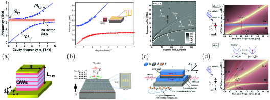
Figure 4: Solid-state CQED setups and their spectral features changing as they approach the single-dipole nonlinear regime. (a) ISB polariton experimental setup and transmission spectrum, taken from Ref. [112]. (b) Landau polariton setup and transmission spectrum, taken from Ref. [113]. (c) Magnonic setup and transmission spectrum, taken from Ref. [114]. (d) Comparison between collective and single particle transmission spectrum, taken from Ref. [115].

6.2 Large $N$ problem

What impact the linearity of the Dicke model has on the possibility of modifying ground-state properties is not immediately clear, given the multitude of possible interactions between the dipolar degree of freedom coupled to the photonic field and all the other internal degrees of freedom of the quantum emitter. Analyzing different simplified models, it has been shown that many single-particle effects are not enhanced by the collective coupling and scale with zero or negative powers of $N$ [7, 118, 119], with adverse consequences on the possibility to modify the equilibrium properties of the matter involved [120, 121, 119, 122].

An intuitive explanation behind the lack of an impact of collective USC on the state of a single TLS [118] can be grasped by noticing that, to the lowest order, the energy shift of a coupled collective eigenmode is of order $\Delta E\propto\sqrt{N}\Omega_{\rm R}$, and the maximal change in such an energy when the internal state of one molecule changes is of order $\frac{\partial\Delta E}{\partial N}\propto\frac{\Omega_{\rm R}}{\sqrt{N}}$. The force acting on the single dipole is thus vanishing in the thermodynamics limit $N\rightarrow\infty$.

However, some experimental works showed a change in chemical reactions [14, 8], a shift in the critical temperature of specific material properties [123] or a modification of the macroscopic quantum Hall transport properties [13] when the system is embedded in a resonant cavity. These systems have a significant coupling strength only considering their collective coupling, thus contradicting the theoretical predictions cited above. Other theoretical works have shown that considering more sophisticated and complex models the collective coupling might have a macroscopic effect on the total reaction process or the material properties [124, 125, 126]. The clash between intuitive results, experimental facts, and complex ab-initio calculations has opened a debate that is still unsolved.

7 Open quantum systems: can we measure the non-empty vacuum?

The photon flux leaking out of a resonator can be usually approximated as the number of photons in the cavity times their escape rate. The presence of photons in the ground state predicted by the USC regime (see Eq. 15) immediately shows how such an intuitive picture fails in this non-perturbative regime, which would otherwise predict photonic emission from the ground state, breaking energy conservation.

Multiple approaches have been developed to correctly deal with such an issue  [127, 74, 128, 129, 130, 131]. Without getting into the technical details required to understand the subtle differences between these various approaches, we will try here to build an intuition of the problem with the standard approaches to open quantum systems. To this aim we will consider the standard Lindblad master equation describing the evolution of the density matrix of a system coupled to a zero temperature reservoir, leading to a loss rate $\gamma$

$$\mathcal{L}_{\mathrm{std}}\hat{\rho}=\gamma\mathcal{D}\left[\hat{S}\right]\hat{\rho},$$ (21)

where $\hat{S}$ is the operator describing the loss of a bare excitation in the system, the Lindblad dissipator is defined as

$$\mathcal{D}\left[\hat{S}\right]\hat{\rho}=\frac{1}{2}\left[2\hat{S}\hat{\rho}\hat{S}^{\dagger}-\hat{S}^{\dagger}\hat{S}\hat{\rho}-\hat{\rho}\hat{S}^{\dagger}\hat{S}\right],$$ (22)

and we neglected the part describing unitary evolution. It is easy to verify that if the ground state is the vacuum for the bare excitations, $\hat{S}\ket{G}=0$, then $\mathcal{L}_{\mathrm{std}}\outerproduct{G}{G}=0$ and the ground state is stable against losses. This is the case for example for the JCM ground state when the operator $\hat{S}$ describes a photonic ($\hat{a}$) or matter ($\hat{\sigma}_{-}$ ) loss

$$\hat{a}\ket{G_{\text{JC}}}=\hat{\sigma}_{-}\ket{G_{\text{JC}}}=0.$$ (23)

This is not the case anymore when the ground state is not the vacuum for the bare excitations $\hat{S}\ket{G}\neq 0$, as clearly shown in Eq. 15 for the Rabi model. This leads to $\mathcal{L}_{\mathrm{std}}\outerproduct{G_{\text{R}}}{G_{\text{R}}}\neq 0$ and the ground state is unstable against losses.

The issue lies in the details of the master equation derivation, which is derived using the bare basis ($\{g,e\}\otimes\{n\in\mathbb{N}\}$) rather than in the energy eigenbasis, and assumes a white reservoir whose density of states can be considered constant in the spectral interval of reference. While these are usually safe approximations, they catastrophically fail in the USC regime, where the energy shifts are of the same order as the bare frequencies. In these conditions, a fully white reservoir implicitly assumes to have a non-vanishing density of states also at negative energies, which explains the instability of the ground state as the emission of unphysical negative-energy excitations in the reservoir.

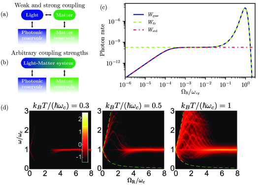
Figure 5: (a) Schematic description of an open hybrid system whose subparts are in weak interaction. (b) The same as before, but this time the two subsystems are ultrastrongly coupled, and the model of the interaction with the environment must take into account their hybridization. (c) Comparison of three different methods to describe open quantum systems, showing the photon emission rate at the steady-state as a function of the vacuum Rabi frequency $\Omega_{\mathrm{R}}$. The generalized master equation is the only one that works across all values of the coupling. (d) The logscale intensity of the spectrally resolved black-body radiation emitted from a cavity QED system as a function of the light-matter coupling. While for intermediate couplings the two polaritonic branches are well visible, deep in the USC regime the spectrum collapses to the uncoupled cavity emission spectrum. Figure taken from Ref. [119].

This problem can be solved by not performing the white-reservoir approximation and deriving the Liouvillian in the eigenbasis of the light-matter Hamiltonian [132]. The resulting dressed master equation takes the form

$$\begin{split}\mathcal{L}^{\prime}\hat{\rho}=&\sum_{j,k}\gamma(\omega_{jk})\mathcal{D}\left[\outerproduct{k}{j}\right]\hat{\rho},\end{split}$$ (24)

where the dissipator is expressed in terms of jump operators between the $k$-th and the $j$-th eigenstates of the coupled light-matter Hamiltonian, $\outerproduct{k}{j}$, with the associated Bohr frequency $\omega_{jk}=\omega_{j}-\omega_{k}$. The vanishing density of states of the bath at negative frequencies then leads to $\gamma(\omega<0)=0$, solving the problem of energy conservation. As a consequence, the open dynamics must be interpreted as transitions between the true eigenstates, where light and matter are entangled together and it is not possible to simply distinguish them separately, as schematized in Fig. 5(a-b)

A problem with this formulation can nevertheless emerge when using it in the weak coupling regime, due to the degenerate nature of the spectrum in such a regime. This in turn led to the derivation of generalized master equations  [130] explicitly taking these degeneracies into account and leading to correct results for all values of the light-matter coupling.

Although the dressed and the generalized master equations at zero temperature lead the system to the ground state, the detection of each quantity can still lead to major mistakes due to the possibly wrong representation of the observables. As a concrete example, we show how the photodetection has to be revised in the USC. Indeed, we already mentioned that $\langle\mathrm{G}_{\mathrm{R}}|\hat{a}^{\dagger}\hat{a}|\mathrm{G}_{\mathrm{R}}\rangle\neq 0$. This suggests that $\hat{a}^{\dagger}\hat{a}$ can no longer be interpreted as the output photon rate, otherwise, we would have photon emission even in the ground state. Following the standard theory of photodetection [133, 134, 135], the output photon rate for a light-matter system in the generic state $|\Psi\rangle$ is proportional to

$$W\propto\matrixelement{\Psi}{\hat{E}^{-}\hat{E}^{+}}{\Psi}\,,$$ (25)

where $\hat{E}^{+}$ ($\hat{E}^{-}=(\hat{E}^{+})^{\dagger}$) is the positive (negative) frequency part of the electric field operator. In case of weak coupling we have $\hat{E}^{+}\propto\hat{a}$ and we obtain the usual formula. In the USC regime, however, we have a hybridization of the frequencies and the positive frequency operator becomes

$$\hat{E}^{+}=\sum_{k>j}\matrixelement{j}{\hat{E}}{k}\outerproduct{j}{k}\,,$$ (26)

which gives $\langle\mathrm{G}_{\mathrm{R}}|\hat{E}^{-}\hat{E}^{+}|\mathrm{G}_{\mathrm{G}}\rangle=0$. Moreover, the form of the electric field operator becomes gauge dependent [119, 136, 137], but leaving the photon rate in Eq. 25 gauge-invariant.

Aside from the correct formalism to adopt, these issues make us to reflect on the meaning of photons in the presence of matter, a point that was raised already a while ago [138]. Virtual photons arising from the USC to matter cannot be simply interpreted as quanta of the transverse electric field oscillations, as commonly done in the free space case. Their physical meaning depends on the gauge that we adopt to describe the interaction with matter and it must be handled with care [32, 94, 139, 140].

In order to provide a concrete example of the formalism introduced here, in Fig. 5(c) we show results for the rate of emitted photons out of a Rabi model where both the cavity and the two-level atom are in interaction with their respective environment. The cavity reservoir is at zero temperature ($T_{c}=0$), while that of the atom has a relatively low temperature $T_{a}=0.05\hbar\omega_{eg}/k_{\mathrm{B}}$. The atom environment is the only source of energy (thermal pumping), and thus the emitted photons are only the result of interaction with the atom. The results are shown for the standard (std), dressed (dr), and generalized (gme) master equations, clearly showing their respective regions of applicability. The well-known Purcell effect [141] is clearly visible in the weak coupling region, where the photon emission rate increases with $\Omega_{\mathrm{R}}$. The signature of the USC can be related to the increase in the photon emission of several orders of magnitude, while the sudden decrease is related to the decoupling effect of the deepstrong coupling regime [61, 142, 143, 101, 84], which will be discussed in details in the next section. In Fig. 5(d) we show the black-body emitted spectrum derived in Ref. [119] within the dressed framework. At low temperatures, for intermediate couplings, the emitted thermal radiation shows the presence of the two polaritonic branches that collapse in a single line at higher coupling strength. Also here we see another manifestation of the non-perturbative light-matter decoupling effect. At higher temperatures, other lines appear at intermediate couplings, before the light-matter decoupling regime, due to non-linear multi-photon transitions, similar to the single-particle transmission spectra from Ref. [115] shown in Fig. 4(d).

8 Recovering the JCM in the deepstrong coupling regime: the light-matter decoupling

After having explored the different ways in which the JCM can break for sufficiently large values of the light-matter coupling, in this last Section we will close the loop, showing how a JCM can be recovered can be recovered for even stronger interaction strengths.

8.1 Light-matter decoupling

One surprising phenomenon of non-perturbative CQED is the so-called light-matter decoupling: while increasing the coupling strength between light and matter typically makes their dynamics more correlated and entangled, for $\Omega_{\rm R}>\omega_{c},\omega_{eg}$ this trend is reversed, and light and matter are rapidly decoupled. As already anticipated in the previous section this feature is well visible in Fig. 5 where the photonemission rate drops to zero at large coupling strength.

The light-matter decoupling was first reported in Ref. [61] in the context of harmonic polariton systems where it was interpreted as a metallization of the optical response of a dielectric for extreme values of the dipolar moment. The dipoles then become perfect metallic mirrors and expel the electromagnetic field (inset in Fig. 6(a) ). This first prediction was indirectly confirmed in Ref. [144]. One important prediction of Ref. [61], shown in Fig. 6(a) is that the Purcell effect [141] breaks down in the USC regime, and the spontaneous emission rate changes non-monotonically with the light-matter coupling, an effect experimentally measured in Ref. [143] and reported in Fig. 6(b).

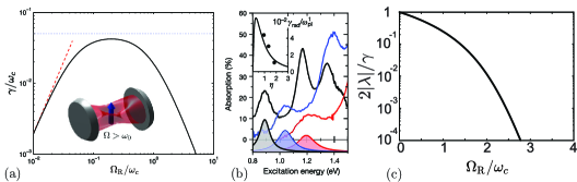
Figure 6: (a) Theoretically predicted electroluminescence emission rate as a function of the coupling strength, taken from Ref. [61]. (b) Experimentally measured absorption spectra of a plasmonic nanoparticle setup in the USC regime and (in the inset) its radiative damping rate as a function of the light-matter coupling strength, taken from Ref. [143]. (c) Liouvillian gap of the open-dissipative Rabi model as a function of the coupling strength, taken from [84].

The USC light-matter decoupling was also investigated in the context of superconducting circuit QED, for instance in Ref. [142, 31], exhibiting a very similar phenomenology. Another related consequence was illustrated and generalized in Ref. [84], where is predicted an exponential slow-down in the thermalization and relaxation dynamics of any USC system. Its quantification can be deduced by the Liouvillian gap [145] of the USC master equation described in the previous section (see Fig. 6(c)).

8.2 The gRWA and the polaronic JCM

The origin of the USC light-matter decoupling in single mode systems can be traced back to the existence of a hidden approximation: the generalized rotating-wave approximation (gRWA). As it was first reported in Ref. [146] and then developed in Ref. [147], it is possible to recover the simple physics of the JCM when the coupling strength places the system deep into the USC regime, where $\Omega_{\rm R}/\omega_{c}\gg 1$. As a consequence, and apparently contradicting what we reported in the previous Sections, the ground state of the system appears as a trivial empty vacuum.

The gRWA is not the standard RWA that leads to the JCM because it first requires transforming the Rabi Hamiltonian in Eq. (13) in a new basis, often called polaron frame. The coordinate transformation is implemented by the same unitary transformation in Eq. (19) which was used to implement the minimal substitution in the Coulomb gauge Hamiltonian directly in the truncated two-level subspace. In this context, unrelated to gauge choices, this transformation is known as polaron transformation. The polaron frame Rabi Hamiltonian (which coincides with the Coulomb gauge TLS Hamiltonian presented at the end of Sec. 5) is then given by

$$\hat{H}_{\rm R}^{\rm pol}=\hat{U}^{{\dagger}}\hat{H}_{\rm R}\hat{U}=\omega_{c}\hat{a}^{{\dagger}}\hat{a}+\frac{\omega_{eg}}{2}\left[\cos\hat{\theta}\hat{\sigma}_{z}-\sin\hat{\theta}\hat{\sigma}_{y}\right],$$ (27)

where $\hat{\theta}=-i2\Omega_{\rm R}/\omega_{c}(\hat{a}-\hat{a}^{{\dagger}})$. At this point, one can Taylor expand the trigonometric operators considering that $\cos\hat{\theta}=(\hat{U}_{D}(\Omega_{\rm R}/\omega_{c})+\hat{U}_{D}(\Omega_{\rm R}/\omega_{c})^{{\dagger}})/2$ and $\sin\hat{\theta}=-i(\hat{U}_{D}(\Omega_{\rm R}/\omega_{c})-\hat{U}_{D}(\Omega_{\rm R}/\omega_{c})^{{\dagger}})/2$ [146, 147, 84]. These operators are expressed in terms of displacement operators $\hat{U}_{D}=\exp[(x^{*}\hat{a}-x\hat{a}^{{\dagger}})]$, allowing for a normal order expansion [148] that permits to easily isolate the positive/negative frequency contributions. After some tedious but straightforward passages, one can re-express the interaction Hamiltonian in a JCM-like form [146, 147, 84]

$$\hat{H}_{\rm R}^{\rm pol}\approx\,\omega_{eg}e^{-2\Omega_{\rm R}^{2}/\omega_{c}^{2}}\left[f(\hat{a}^{{\dagger}}\hat{a})\hat{a}\hat{\sigma}_{+}+f^{*}(\hat{a}^{{\dagger}}\hat{a})\hat{a}^{{\dagger}}\hat{\sigma}_{-}\right],$$ (28)

where $f$ is a complicated polynomial function [146]. This expression is still mathematically very complicated but has the advantage of clearly showing that also the Rabi model is mostly built over the concept of absorption/emission. The exponential coefficient in front $e^{-2\Omega_{\rm R}^{2}/\omega_{c}^{2}}$ emerges also as a feature of the polaron transformation and explicitly accounts for the light-matter decoupling in the infinite coupling limit $\Omega_{\rm R}\rightarrow\infty$. It also explains why the gRWA is applicable in such a limit, suppressing the polaron light-matter interaction term which is then treated in perturbation theory, similarly to what is introduced in Sec. 2.

As a specific property, the ground state in the polaron frame is given by $|{\rm G}_{\rm pol}\rangle\approx|0,g\rangle$ being indeed the empty cavity vacuum. To obtain the ground state in the standard frame (or Rabi vacuum) we have to transform this state back, obtaining

$$|{\rm G}_{\rm R}\rangle\approx\hat{U}|0,g\rangle=\frac{1}{\sqrt{2}}\left(|\alpha,\rightarrow\rangle+|-\alpha,\leftarrow\rangle\right),$$ (29)

where $|\alpha\rangle$ is a photon’s coherent state with amplitude $\alpha=\Omega_{\rm R}/\omega_{c}$ and $|\leftarrow/\rightarrow\rangle=(|e\rangle\pm|g\rangle)/\sqrt{2}$. We then notice that all the notions of vacuum and virtual photons are only relative to the specific considered frame (or Hilbert space basis). Moreover, we see that the Rabi vacuum is not only non-empty but is also highly entangled since for $\Omega_{\rm R}\gg\omega_{c}$ it is a cat state [1]. In the polaron basis, the ground state instead becomes quite trivial and loses all the entanglement (which is also a relative property). This observation stimulated the idea that in light-matter problems one can always find a disentangling transformation that strongly simplifies the description. In particular, this was explored in multimodal light-matter systems, where the polaron transformation is generalized to treat the USC regime on the basis of minimizing the entanglement between matter and light. In Ref. [149, 150] is shown that a generalized polaron transformation can be used to extract semi-analytical approximated solutions of the multi-mode USC systems.

9 Conclusion

In this paper, we tried to provide a non-technical report on the relevance of the JCM in the contemporary research landscape. The vitality of such a topic of investigation can be easily gauged by the fact that essentially all the approximations on which the JCM rests have been tested, stretched, and broken in one way or another. The JCM remains today an important toy model to approach the topic of light-matter coupling at the quantum level. Still, it is best understood as one node of various related models, mapping a much broader section of the parameter space and hosting a corresponding much-richer phenomenology, which we are sure will continue to fascinate researchers for many years to come.

Funding S.D.L. acknowledges funding from the Leverhulme Trust through the grant RPG-2022-037 and the Philip Leverhulme Prize. D.D.B. acknowledges funding from the European Union - NextGeneration EU, "Integrated infrastructure initiative in Photonic and Quantum Sciences" - I-PHOQS [IR0000016, ID D2B8D520, CUP B53C22001750006].

Disclosures The authors declare no conflicts of interest.

Data availability No data were generated or analyzed in the presented research.

References

- [1] S. Haroche, “Nobel Lecture: Controlling photons in a box and exploring the quantum to classical boundary,” \JournalTitleRev. Mod. Phys. 85, 1083 (2013).
- [2] D. J. Wineland, “Nobel Lecture: Superposition, entanglement, and raising Schr\"odinger’s cat,” \JournalTitleReviews of Modern Physics 85, 1103–1114 (2013).
- [3] A. V. Zasedatelev, A. V. Baranikov, D. Urbonas, et al., “A room-temperature organic polariton transistor,” \JournalTitleNature Photonics 13, 378–383 (2019).
- [4] N. G. Berloff, M. Silva, K. Kalinin, et al., “Realizing the classical XY Hamiltonian in polariton simulators,” \JournalTitleNature Materials 16, 1120 (2017).
- [5] D. Ballarini, A. Gianfrate, R. Panico, et al., “Polaritonic Neuromorphic Computing Outperforms Linear Classifiers,” \JournalTitleNano Letters 20, 3506–3512 (2020).
- [6] T. Schwartz, J. A. Hutchison, C. Genet, and T. W. Ebbesen, “Reversible Switching of Ultrastrong Light-Molecule Coupling,” \JournalTitlePhys. Rev. Lett. 106, 196405 (2011).
- [7] J. A. Ćwik, P. Kirton, S. De Liberato, and J. Keeling, “Excitonic spectral features in strongly coupled organic polaritons,” \JournalTitlePhys. Rev. A 93, 033840 (2016).
- [8] K. Nagarajan, A. Thomas, and T. W. Ebbesen, “Chemistry under Vibrational Strong Coupling,” \JournalTitleJournal of the American Chemical Society 143, 16877–16889 (2021). Publisher: American Chemical Society.
- [9] M. Nomura, N. Kumagai, S. Iwamoto, et al., “Laser oscillation in a strongly coupled single-quantum-dot–nanocavity system,” \JournalTitleNature Physics 6, 279–283 (2010).
- [10] A. Delteil, T. Fink, A. Schade, et al., “Towards polariton blockade of confined exciton–polaritons,” \JournalTitleNature Materials 18, 219–222 (2019). Number: 3 Publisher: Nature Publishing Group.
- [11] S. Brodbeck, S. De Liberato, M. Amthor, et al., “Experimental Verification of the Very Strong Coupling Regime in a GaAs Quantum Well Microcavity,” \JournalTitlePhys. Rev. Lett. 119, 027401 (2017).
- [12] E. Cortese, N.-L. Tran, J.-M. Manceau, et al., “Excitons bound by photon exchange,” \JournalTitleNature Physics 17, 31–35 (2021).
- [13] F. Appugliese, J. Enkner, G. L. Paravicini-Bagliani, et al., “Breakdown of topological protection by cavity vacuum fields in the integer quantum Hall effect,” \JournalTitleScience 375, 1030–1034 (2022). Publisher: American Association for the Advancement of Science.
- [14] F. J. Garcia-Vidal, C. Ciuti, and T. W. Ebbesen, “Manipulating matter by strong coupling to vacuum fields,” \JournalTitleScience 373, eabd0336 (2021).
- [15] D. De Bernardis, M. Jeannin, J.-M. Manceau, et al., “Magnetic-field-induced cavity protection for intersubband polaritons,” \JournalTitlePhysical Review B 106, 224206 (2022).
- [16] A. Einstein, “Volume 6: The Berlin Years: Writings, 1914-1917 (English translation supplement) page 212,” .
- [17] J. Larson and T. Mavrogordatos, The Jaynes–Cummings Model and Its Descendants: Modern research directions (IOP Publishing, 2021).
- [18] S. Haroche and J.-M. Raimond, Exploring the quantum: atoms, cavities, and photons, Oxford graduate texts (Oxford University Press, Oxford, 2013), first published in paperback ed.
- [19] F. Yoshihara, T. Fuse, S. Ashhab, et al., “Superconducting qubit–oscillator circuit beyond the ultrastrong-coupling regime,” \JournalTitleNature Physics 13, 44 EP – (2016).
- [20] F. Valmorra, K. Yoshida, L. C. Contamin, et al., “Vacuum-field-induced THz transport gap in a carbon nanotube quantum dot,” \JournalTitleNature Communications 12, 5490 (2021).
- [21] R. Chikkaraddy, B. de Nijs, F. Benz, et al., “Single-molecule strong coupling at room temperature in plasmonic nanocavities,” \JournalTitleNature 535, 127–130 (2016).
- [22] H. J. Kimble and T. W. Lynn, “Cavity QED with Strong Coupling — Toward the Deterministic Control of Quantum Dynamics,” in Coherence and Quantum Optics VIII, N. P. Bigelow, J. H. Eberly, C. R. Stroud, and I. A. Walmsley, eds. (Springer US, Boston, MA, 2003), pp. 45–54.
- [23] P. Forn-Díaz, L. Lamata, E. Rico, et al., “Ultrastrong coupling regimes of light-matter interaction,” \JournalTitleRev. Mod. Phys. 91, 025005 (2019).
- [24] A. Frisk Kockum, A. Miranowicz, S. De Liberato, et al., “Ultrastrong coupling between light and matter,” \JournalTitleNature Reviews Physics 1, 19–40 (2019).
- [25] A. Le Boité, “Theoretical Methods for Ultrastrong Light–Matter Interactions,” \JournalTitleAdvanced Quantum Technologies 3, 1900140 (2020).
- [26] D. Z. Rossatto, C. J. Villas-Bôas, M. Sanz, and E. Solano, “Spectral classification of coupling regimes in the quantum Rabi model,” \JournalTitlePhys. Rev. A 96, 013849 (2017).
- [27] A. A. Anappara, S. De Liberato, A. Tredicucci, et al., “Signatures of the ultrastrong light-matter coupling regime,” \JournalTitlePhys. Rev. B 79, 201303 (2009).
- [28] M. H. Devoret, S. Girvin, and R. Schoelkopf, “Circuit-QED: How strong can the coupling between a Josephson junction atom and a transmission line resonator be?” \JournalTitleAnn. Phys. 16, 767 (2007).
- [29] J. B. Khurgin, “How to deal with the loss in plasmonics and metamaterials,” \JournalTitleNature Nanotechnology 10, 2 EP – (2015).
- [30] T. Niemczyk, F. Deppe, H. Huebl, et al., “Circuit quantum electrodynamics in the ultrastrong-coupling regime,” \JournalTitleNat. Phys. 6, 772 (2010).
- [31] T. Jaako, Z.-L. Xiang, J. J. Garcia-Ripoll, and P. Rabl, “Ultrastrong-coupling phenomena beyond the Dicke model,” \JournalTitlePhys. Rev. A 94, 033850 (2016).
- [32] D. De Bernardis, T. Jaako, and P. Rabl, “Cavity quantum electrodynamics in the nonperturbative regime,” \JournalTitlePhys. Rev. A 97, 043820 (2018).
- [33] R. Sáez-Blázquez, D. de Bernardis, J. Feist, and P. Rabl, “Can We Observe Nonperturbative Vacuum Shifts in Cavity QED?” \JournalTitlePhysical Review Letters 131, 013602 (2023).
- [34] M. Kuisma, B. Rousseaux, K. M. Czajkowski, et al., “Ultrastrong Coupling of a Single Molecule to a Plasmonic Nanocavity: A First-Principles Study,” \JournalTitleACS Photonics 9, 1065–1077 (2022).
- [35] P. Forn-Díaz, J. J. García-Ripoll, B. Peropadre, et al., “Ultrastrong coupling of a single artificial atom to an electromagnetic continuum in the nonperturbative regime,” \JournalTitleNat. Phys. 13, 39 (2017).
- [36] S.-P. Wang, A. Mercurio, A. Ridolfo, et al., “Strong coupling between a single photon and a photon pair,” (2024). ArXiv:2401.02738 [quant-ph].
- [37] N. Mehta, R. Kuzmin, C. Ciuti, and V. E. Manucharyan, “Down-conversion of a single photon as a probe of many-body localization,” \JournalTitleNature 613, 650–655 (2023).
- [38] A. Tomonaga, R. Stassi, H. Mukai, et al., “One photon simultaneously excites two atoms in a ultrastrongly coupled light-matter system,” (2024). ArXiv:2307.15437 [quant-ph].
- [39] A. Vrajitoarea, R. Belyansky, R. Lundgren, et al., “Ultrastrong light-matter interaction in a multimode photonic crystal,” (2024). ArXiv:2209.14972 [cond-mat, physics:quant-ph].
- [40] F. Benz, M. K. Schmidt, A. Dreismann, et al., “Single-molecule optomechanics in “picocavities”,” \JournalTitleScience 354, 726–729 (2016).
- [41] L. A. Jakob, W. M. Deacon, Y. Zhang, et al., “Giant optomechanical spring effect in plasmonic nano- and picocavities probed by surface-enhanced Raman scattering,” \JournalTitleNature Communications 14, 3291 (2023).
- [42] C. Cohen-Tannoudji, J. Dupont-Roc, and G. Grynberg, “Lagrangian and Hamiltonian Approach to Electrodynamics, The Standard Lagrangian and the Coulomb Gauge,” in Photons and Atoms, (John Wiley and Sons, Ltd, 1997), pp. 79–168. Section: 2 _eprint: https://onlinelibrary.wiley.com/doi/pdf/10.1002/9783527618422.ch2.
- [43] A. Stokes and A. Nazir, “Identification of Poincar\’e-gauge and multipolar nonrelativistic theories of QED,” \JournalTitlePhysical Review A 104, 032227 (2021).
- [44] D. P. Craig and T. Thirunamachandran, Molecular quantum electrodynamics: an introduction to radiation-molecule interactions (Dover Publications, Mineola, N.Y, 1998).
- [45] M. L. Andersen, S. Stobbe, A. S. Sørensen, and P. Lodahl, “Strongly modified plasmon–matter interaction with mesoscopic quantum emitters,” \JournalTitleNature Physics 7, 215–218 (2011).
- [46] P. Tighineanu, S. Stobbe, and P. Lodahl, “Accessing the Magnetic Dipole and Electric Quadrupole of Quantum Dots with Light,” in CLEO: 2014 (2014), paper FF2K.6, (Optica Publishing Group, 2014), p. FF2K.6.
- [47] S. Raza, S. Kadkhodazadeh, T. Christensen, et al., “Multipole plasmons and their disappearance in few-nanometre silver nanoparticles,” \JournalTitleNature Communications 6, 8788 (2015). Number: 1 Publisher: Nature Publishing Group.
- [48] P. Anger, P. Bharadwaj, and L. Novotny, “Enhancement and Quenching of Single-Molecule Fluorescence,” \JournalTitlePhysical Review Letters 96, 113002 (2006). Publisher: American Physical Society.
- [49] S. Felicetti, M.-J. Hwang, and A. Le Boité, “Ultrastrong-coupling regime of nondipolar light-matter interactions,” \JournalTitlePhysical Review A 98, 053859 (2018).
- [50] J. V. Koski, A. J. Landig, M. Russ, et al., “Strong photon coupling to the quadrupole moment of an electron in a solid-state qubit,” \JournalTitleNature Physics 16, 642–646 (2020).
- [51] D. De Bernardis, P. Pilar, T. Jaako, et al., “Breakdown of gauge invariance in ultrastrong-coupling cavity QED,” \JournalTitlePhysical Review A 98, 053819 (2018).
- [52] J. B. Khurgin, “Excitonic radius in the cavity polariton in the regime of very strong coupling,” \JournalTitleSolid State Communications 117, 307–310 (2001).
- [53] B. Askenazi, A. Vasanelli, A. Delteil, et al., “Ultra-strong light–matter coupling for designer Reststrahlen band,” \JournalTitleNew Journal of Physics 16, 043029 (2014).
- [54] E. Cortese, I. Carusotto, R. Colombelli, and S. De Liberato, “Strong coupling of ionizing transitions,” \JournalTitleOptica 6, 354 (2019).
- [55] J. Levinsen, G. Li, and M. M. Parish, “Microscopic description of exciton-polaritons in microcavities,” \JournalTitlePhysical Review Research 1, 033120 (2019).
- [56] C. R. Gubbin, S. A. Maier, and S. De Liberato, “Real-space Hopfield diagonalization of inhomogeneous dispersive media,” \JournalTitlePhys. Rev. B 94, 205301 (2016).
- [57] R. Kuzmin, N. Mehta, N. Grabon, et al., “Superstrong coupling in circuit quantum electrodynamics,” \JournalTitlenpj Quantum Information 5, 1–6 (2019). Number: 1 Publisher: Nature Publishing Group.
- [58] C. Sánchez Muñoz, F. Nori, and S. De Liberato, “Resolution of superluminal signalling in non-perturbative cavity quantum electrodynamics,” \JournalTitleNature Communications 9, 1924 (2018).
- [59] E. Cortese, J. Mornhinweg, R. Huber, et al., “Real-space nanophotonic field manipulation using non-perturbative light–matter coupling,” \JournalTitleOptica 10, 11–19 (2023). Publisher: Optica Publishing Group.
- [60] J. Mornhinweg, L. Diebel, M. Halbhuber, et al., “Sculpting ultrastrong light–matter coupling through spatial matter structuring,” \JournalTitleNanophotonics (2024). Publisher: De Gruyter.
- [61] S. De Liberato, “Light-Matter Decoupling in the Deep Strong Coupling Regime: The Breakdown of the Purcell Effect,” \JournalTitlePhys. Rev. Lett. 112, 016401 (2014).
- [62] D. Braak, “Integrability of the Rabi Model,” \JournalTitlePhysical Review Letters 107, 100401 (2011).
- [63] J. Casanova, G. Romero, I. Lizuain, et al., “Deep Strong Coupling Regime of the Jaynes-Cummings Model,” \JournalTitlePhys. Rev. Lett. 105, 263603 (2010).
- [64] F. A. Wolf, F. Vallone, G. Romero, et al., “Dynamical correlation functions and the quantum Rabi model,” \JournalTitlePhys. Rev. A 87, 023835 (2013).
- [65] P. Forn-Díaz, G. Romero, C. J. P. M. Harmans, et al., “Broken selection rule in the quantum Rabi model,” \JournalTitleSci. Rep. 6, 26720 (2016).
- [66] O. D. Stefano, R. Stassi, L. Garziano, et al., “Feynman-diagrams approach to the quantum Rabi model for ultrastrong cavity QED: stimulated emission and reabsorption of virtual particles dressing a physical excitation,” \JournalTitleNew Journal of Physics 19, 053010 (2017).
- [67] J. R. Johansson, P. D. Nation, and F. Nori, “QuTiP 2: A Python framework for the dynamics of open quantum systems,” \JournalTitleComputer Physics Communications 184, 1234–1240 (2013).
- [68] P. Forn-Díaz, J. Lisenfeld, D. Marcos, et al., “Observation of the Bloch-Siegert Shift in a Qubit-Oscillator System in the Ultrastrong Coupling Regime,” \JournalTitlePhys. Rev. Lett. 105, 237001 (2010).
- [69] X. Li, M. Bamba, Q. Zhang, et al., “Vacuum Bloch–Siegert shift in Landau polaritons with ultra-high cooperativity,” \JournalTitleNature Photonics 12, 324–329 (2018).
- [70] C. Ciuti, G. Bastard, and I. Carusotto, “Quantum vacuum properties of the intersubband cavity polariton field,” \JournalTitlePhysical Review B 72, 115303 (2005).
- [71] E. V. Shuryak, “The QCD vacuum and quark-gluon plasma,” in Quark Matter, H. Satz, H. J. Specht, and R. Stock, eds. (Springer, Berlin, Heidelberg, 1988), pp. 141–145.
- [72] P. W. Milonni, The quantum vacuum: an introduction to quantum electrodynamics (Academic Press, Boston, 1994).
- [73] Y. Wang and S. De Liberato, “Theoretical proposals to measure resonator-induced modifications of the electronic ground state in doped quantum wells,” \JournalTitlePhysical Review A 104, 023109 (2021).
- [74] S. De Liberato, D. Gerace, I. Carusotto, and C. Ciuti, “Extracavity quantum vacuum radiation from a single qubit,” \JournalTitlePhys. Rev. A 80, 053810 (2009).
- [75] M. Cirio, S. De Liberato, N. Lambert, and F. Nori, “Ground State Electroluminescence,” \JournalTitlePhys. Rev. Lett. 116, 113601 (2016).
- [76] J. Lolli, A. Baksic, D. Nagy, et al., “Ancillary Qubit Spectroscopy of Vacua in Cavity and Circuit Quantum Electrodynamics,” \JournalTitlePhysical Review Letters 114, 183601 (2015).
- [77] D. De Bernardis, G. M. Andolina, and I. Carusotto, “Light-matter interactions in the vacuum of ultra-strongly coupled systems,” (2023). ArXiv:2312.16287 [cond-mat, physics:quant-ph].
- [78] F. Minganti, A. Mercurio, F. Mauceri, et al., “Phonon Pumping by Modulating the Ultrastrong Vacuum,” (2023). ArXiv:2309.15891 [quant-ph].
- [79] K. K. W. Ma and C. K. Law, “Three-photon resonance and adiabatic passage in the large-detuning Rabi model,” \JournalTitlePhysical Review A 92, 023842 (2015).
- [80] A. Blais, A. L. Grimsmo, S. Girvin, and A. Wallraff, “Circuit quantum electrodynamics,” \JournalTitleReviews of Modern Physics 93, 025005 (2021).
- [81] L. Garziano, R. Stassi, V. Macrì, et al., “Multiphoton quantum Rabi oscillations in ultrastrong cavity QED,” \JournalTitlePhys. Rev. A 92, 063830 (2015).
- [82] A. F. Kockum, A. Miranowicz, V. Macrì, et al., “Deterministic quantum nonlinear optics with single atoms and virtual photons,” \JournalTitlePhys. Rev. A 95, 063849 (2017).
- [83] S. Felicetti, D. Z. Rossatto, E. Rico, et al., “Two-photon quantum Rabi model with superconducting circuits,” \JournalTitlePhysical Review A 97, 013851 (2018).
- [84] D. De Bernardis, “Relaxation breakdown and resonant tunneling in ultrastrong-coupling cavity QED,” \JournalTitlePhysical Review A 108, 043717 (2023).
- [85] J. Koch, F. von Oppen, and A. V. Andreev, “Theory of the Franck-Condon blockade regime,” \JournalTitlePhysical Review B 74, 205438 (2006).
- [86] R. Leturcq, C. Stampfer, K. Inderbitzin, et al., “Franck–Condon blockade in suspended carbon nanotube quantum dots,” \JournalTitleNature Physics 5, 327–331 (2009).
- [87] Y. Cui, S. Tosoni, W.-D. Schneider, et al., “Phonon-Mediated Electron Transport through CaO Thin Films,” \JournalTitlePhysical Review Letters 114, 016804 (2015).
- [88] E. Vdovin, A. Mishchenko, M. Greenaway, et al., “Phonon-Assisted Resonant Tunneling of Electrons in Graphene–Boron Nitride Transistors,” \JournalTitlePhysical Review Letters 116, 186603 (2016).
- [89] V. Macrì, A. Mercurio, F. Nori, et al., “Spontaneous Scattering of Raman Photons from Cavity-QED Systems in the Ultrastrong Coupling Regime,” \JournalTitlePhysical Review Letters 129, 273602 (2022).
- [90] K. Koshino, T. Shitara, Z. Ao, and K. Semba, “Deterministic three-photon down-conversion by a passive ultrastrong cavity-QED system,” \JournalTitlePhysical Review Research 4, 013013 (2022).
- [91] N. Mehta, C. Ciuti, R. Kuzmin, and V. E. Manucharyan, “Theory of strong down-conversion in multi-mode cavity and circuit QED,” (2022). ArXiv:2210.14681 [cond-mat, physics:quant-ph].
- [92] W. E. Lamb, “Fine Structure of the Hydrogen Atom. III,” \JournalTitlePhys. Rev. 85, 259–276 (1952). Number: 2 Publisher: American Physical Society.
- [93] F. Bassani, J. J. Forney, and A. Quattropani, “Choice of Gauge in Two-Photon Transitions: 1s\ensuremath-2s Transition in Atomic Hydrogen,” \JournalTitlePhys. Rev. Lett. 39, 1070–1073 (1977). Number: 17 Publisher: American Physical Society.
- [94] A. Stokes and A. Nazir, “Gauge ambiguities imply Jaynes-Cummings physics remains valid in ultrastrong coupling QED,” \JournalTitleNature Communications 10, 499 (2019).
- [95] O. Di Stefano, A. Settineri, V. Macrì, et al., “Resolution of gauge ambiguities in ultrastrong-coupling cavity quantum electrodynamics,” \JournalTitleNature Physics 15, 803–808 (2019).
- [96] M. A. D. Taylor, A. Mandal, W. Zhou, and P. Huo, “Resolution of Gauge Ambiguities in Molecular Cavity Quantum Electrodynamics,” \JournalTitlePhysical Review Letters 125, 123602 (2020).
- [97] A. Stokes and A. Nazir, “Implications of gauge freedom for nonrelativistic quantum electrodynamics,” \JournalTitleReviews of Modern Physics 94, 045003 (2022).
- [98] G. Arwas, V. E. Manucharyan, and C. Ciuti, “Metrics and properties of optimal gauges in multimode cavity QED,” \JournalTitlePhysical Review A 108, 023714 (2023).
- [99] M. Babiker and R. Loudon, “Derivation of the Power-Zienau-Woolley Hamiltonian in quantum electrodynamics by gauge transformation,” \JournalTitleProceedings of the Royal Society of London. A. Mathematical and Physical Sciences 385, 439–460 (1983). Number: 1789 Publisher: The Royal Society London.
- [100] J. J. Sakurai and J. Napolitano, Modern quantum mechanics (Cambridge University Press, Cambridge, 2021), 3rd ed.
- [101] Y. Ashida, A. İmamoğlu, and E. Demler, “Cavity Quantum Electrodynamics at Arbitrary Light-Matter Coupling Strengths,” \JournalTitlePhysical Review Letters 126, 153603 (2021).
- [102] Y. Ashida, T. Yokota, A. İmamoğlu, and E. Demler, “Nonperturbative waveguide quantum electrodynamics,” \JournalTitlePhysical Review Research 4, 023194 (2022).
- [103] S. Savasta, O. Di Stefano, A. Settineri, et al., “Gauge principle and gauge invariance in two-level systems,” \JournalTitlePhysical Review A 103, 053703 (2021).
- [104] D. Zueco, G. M. Reuther, S. Kohler, and P. Hänggi, “Qubit-oscillator dynamics in the dispersive regime: Analytical theory beyond the rotating-wave approximation,” \JournalTitlePhysical Review A 80, 033846 (2009).
- [105] V. E. Manucharyan, A. Baksic, and C. Ciuti, “Resilience of the quantum Rabi model in circuit QED,” \JournalTitleJournal of Physics A: Mathematical and Theoretical 50, 294001 (2017).
- [106] J. Bloch, A. Cavalleri, V. Galitski, et al., “Strongly correlated electron–photon systems,” \JournalTitleNature 606, 41–48 (2022).
- [107] M. Lagrée, M. Jeannin, G. Quinchard, et al., “An effective density matrix approach for intersubband plasmons coupled to a cavity field: electrical extraction/injection of intersubband polaritons,” (2023). ArXiv:2307.05472 [cond-mat, physics:physics].
- [108] F. Pisani, D. Gacemi, A. Vasanelli, et al., “Electronic transport driven by collective light-matter coupled states in a quantum device,” \JournalTitleNature Communications 14, 3914 (2023).
- [109] P. Kirton, M. M. Roses, J. Keeling, and E. G. Dalla Torre, “Introduction to the Dicke Model: From Equilibrium to Nonequilibrium, and Vice Versa,” \JournalTitleAdvanced Quantum Technologies 2, 1800043 (2019).
- [110] T. Holstein and H. Primakoff, “Field Dependence of the Intrinsic Domain Magnetization of a Ferromagnet,” \JournalTitlePhysical Review 58, 1098–1113 (1940).
- [111] A. Klein and E. R. Marshalek, “Boson realizations of Lie algebras with applications to nuclear physics,” \JournalTitleReviews of Modern Physics 63, 375–558 (1991).
- [112] Y. Todorov, A. M. Andrews, R. Colombelli, et al., “Ultrastrong Light-Matter Coupling Regime with Polariton Dots,” \JournalTitlePhys. Rev. Lett. 105, 196402 (2010).
- [113] G. Scalari, C. Maissen, D. Turcinkova, et al., “Ultrastrong Coupling of the Cyclotron Transition of a 2D Electron Gas to a THz Metamaterial,” \JournalTitleScience 335, 1323 (2012).
- [114] I. Golovchanskiy, N. Abramov, V. Stolyarov, et al., “Approaching Deep-Strong On-Chip Photon-To-Magnon Coupling,” \JournalTitlePhysical Review Applied 16, 034029 (2021).
- [115] Y. Todorov and C. Sirtori, “Few-Electron Ultrastrong Light-Matter Coupling in a Quantum LC Circuit,” \JournalTitlePhys. Rev. X 4, 041031 (2014).
- [116] J. Keller, G. Scalari, S. Cibella, et al., “Few-Electron Ultrastrong Light-Matter Coupling at 300 GHz with Nanogap Hybrid LC Microcavities,” \JournalTitleNano Letters 17, 7410–7415 (2017).
- [117] S. Rajabali, S. Markmann, E. Jöchl, et al., “An ultrastrongly coupled single terahertz meta-atom,” \JournalTitleNature Communications 13, 2528 (2022). Number: 1 Publisher: Nature Publishing Group.
- [118] E. Cortese, P. G. Lagoudakis, and S. De Liberato, “Collective Optomechanical Effects in Cavity Quantum Electrodynamics,” \JournalTitlePhys. Rev. Lett. 119, 043604 (2017).
- [119] P. Pilar, D. D. Bernardis, and P. Rabl, “Thermodynamics of ultrastrongly coupled light-matter systems,” \JournalTitleQuantum 4, 335 (2020).
- [120] J. Galego, C. Climent, F. J. Garcia-Vidal, and J. Feist, “Cavity Casimir-Polder Forces and Their Effects in Ground-State Chemical Reactivity,” \JournalTitlePhysical Review X 9, 021057 (2019). Publisher: American Physical Society.
- [121] L. A. Martínez-Martínez, R. F. Ribeiro, J. Campos-González-Angulo, and J. Yuen-Zhou, “Can Ultrastrong Coupling Change Ground-State Chemical Reactions?” \JournalTitleACS Photonics 5, 167–176 (2018). Publisher: American Chemical Society.
- [122] K. S. U. Kansanen, “Theory for polaritonic quantum tunneling,” \JournalTitlePhysical Review B 107, 035405 (2023).
- [123] G. Jarc, S. Y. Mathengattil, A. Montanaro, et al., “Cavity-mediated thermal control of metal-to-insulator transition in 1T-TaS2,” \JournalTitleNature 622, 487–492 (2023).
- [124] C. Schäfer, J. Flick, E. Ronca, et al., “Shining light on the microscopic resonant mechanism responsible for cavity-mediated chemical reactivity,” \JournalTitleNature Communications 13, 7817 (2022).
- [125] K. Lenk, J. Li, P. Werner, and M. Eckstein, “Collective theory for an interacting solid in a single-mode cavity,” (2022). ArXiv:2205.05559 [cond-mat].
- [126] P. Fadler, J. Li, K. P. Schmidt, and M. Eckstein, “Engineering Photon-mediated Long-Range Spin Interactions in Mott Insulators,” (2023). ArXiv:2311.01339 [cond-mat].
- [127] C. Ciuti and I. Carusotto, “Input-output theory of cavities in the ultrastrong coupling regime: The case of time-independent cavity parameters,” \JournalTitlePhys. Rev. A 74, 033811 (2006).
- [128] M. Bamba and T. Ogawa, “System-environment coupling derived by Maxwell’s boundary conditions from the weak to the ultrastrong light-matter-coupling regime,” \JournalTitlePhys. Rev. A 88, 013814 (2013).
- [129] M. Bamba and T. Ogawa, “Recipe for the Hamiltonian of system-environment coupling applicable to the ultrastrong-light-matter-interaction regime,” \JournalTitlePhys. Rev. A 89, 023817 (2014).
- [130] A. Settineri, V. Macrí, A. Ridolfo, et al., “Dissipation and thermal noise in hybrid quantum systems in the ultrastrong-coupling regime,” \JournalTitlePhysical Review A 98, 053834 (2018).
- [131] O. Di Stefano, A. F. Kockum, A. Ridolfo, et al., “Photodetection probability in quantum systems with arbitrarily strong light-matter interaction,” \JournalTitleScientific Reports 8, 17825 (2018).
- [132] F. Beaudoin, J. M. Gambetta, and A. Blais, “Dissipation and ultrastrong coupling in circuit QED,” \JournalTitlePhys. Rev. A 84, 043832 (2011).
- [133] R. J. Glauber, “The Quantum Theory of Optical Coherence,” \JournalTitlePhysical Review 130, 2529–2539 (1963).
- [134] C. Cohen-Tannoudji, J. Dupont-Roc, and G. Grynberg, Atom—Photon Interactions: Basic Process and Appilcations (Wiley, 1998), 1st ed.
- [135] D. Walls and G. J. Milburn, eds., Quantum Optics (Springer, Berlin, Heidelberg, 2008).
- [136] A. Settineri, O. Di Stefano, D. Zueco, et al., “Gauge freedom, quantum measurements, and time-dependent interactions in cavity QED,” \JournalTitlePhysical Review Research 3, 023079 (2021).
- [137] A. Mercurio, V. Macrì, C. Gustin, et al., “Regimes of cavity QED under incoherent excitation: From weak to deep strong coupling,” \JournalTitlePhysical Review Research 4, 023048 (2022).
- [138] W. E. Lamb, “Anti-photon,” \JournalTitleApplied Physics B 60, 77–84 (1995).
- [139] D. M. Rouse, A. Stokes, and A. Nazir, “Theory of photon condensation in an arbitrary-gauge condensed matter cavity model,” \JournalTitlePhysical Review B 107, 205128 (2023).
- [140] A. Stokes, H. Riley, and A. Nazir, “The Gauge-Relativity of Quantum Light, Matter, and Information,” \JournalTitleOpen Systems & Information Dynamics 30, 2350016 (2023).
- [141] E. M. Purcell, H. C. Torrey, and R. V. Pound, “Resonance Absorption by Nuclear Magnetic Moments in a Solid,” \JournalTitlePhysical Review 69, 37–38 (1946).
- [142] J. J. García-Ripoll, B. Peropadre, and S. De Liberato, “Light-matter decoupling and A2 term detection in superconducting circuits,” \JournalTitleScientific Reports 5, 16055 (2015).
- [143] N. S. Mueller, Y. Okamura, B. G. M. Vieira, et al., “Deep strong light–matter coupling in plasmonic nanoparticle crystals,” \JournalTitleNature 583, 780–784 (2020).
- [144] A. Bayer, M. Pozimski, S. Schambeck, et al., “Terahertz Light-Matter Interaction beyond Unity Coupling Strength,” \JournalTitleNano Lett. 17, 6340 (2017).
- [145] F. Minganti, A. Biella, N. Bartolo, and C. Ciuti, “Spectral theory of Liouvillians for dissipative phase transitions,” \JournalTitlePhysical Review A 98, 042118 (2018).
- [146] E. K. Irish, “Generalized Rotating-Wave Approximation for Arbitrarily Large Coupling,” \JournalTitlePhysical Review Letters 99, 173601 (2007).
- [147] L. Yu, S. Zhu, Q. Liang, et al., “Analytical solutions for the Rabi model,” \JournalTitlePhysical Review A 86, 015803 (2012).
- [148] K. E. Cahill and R. J. Glauber, “Ordered Expansions in Boson Amplitude Operators,” \JournalTitlePhysical Review 177, 1857–1881 (1969).
- [149] G. Díaz-Camacho, A. Bermudez, and J. J. García-Ripoll, “Dynamical polaron Ansatz: A theoretical tool for the ultrastrong-coupling regime of circuit QED,” \JournalTitlePhysical Review A 93, 043843 (2016).
- [150] T. Shi, Y. Chang, and J. J. García-Ripoll, “Ultrastrong Coupling Few-Photon Scattering Theory,” \JournalTitlePhysical Review Letters 120, 153602 (2018).