OTClean: Data Cleaning for Conditional Independence Violations using Optimal Transport

Abstract.

Ensuring Conditional Independence (CI) constraints is pivotal for the development of fair and trustworthy machine learning models. In this paper, we introduce OTClean, a framework that harnesses optimal transport theory for data repair under CI constraints. Optimal transport theory provides a rigorous framework for measuring the discrepancy between probability distributions, thereby ensuring control over data utility. We formulate the data repair problem concerning CIs as a Quadratically Constrained Linear Program (QCLP) and propose an alternating method for its solution. However, this approach faces scalability issues due to the computational cost associated with computing optimal transport distances, such as the Wasserstein distance. To overcome these scalability challenges, we reframe our problem as a regularized optimization problem, enabling us to develop an iterative algorithm inspired by Sinkhorn’s matrix scaling algorithm, which efficiently addresses high-dimensional and large-scale data. Through extensive experiments, we demonstrate the efficacy and efficiency of our proposed methods, showcasing their practical utility in real-world data cleaning and preprocessing tasks. Furthermore, we provide comparisons with traditional approaches, highlighting the superiority of our techniques in terms of preserving data utility while ensuring adherence to the desired CI constraints.

1. Introduction

Conditional Independence (CI) plays a pivotal role in probability and statistics. At its core, a CI statement, represented as $(X\mbox{$\perp\!\!\!\perp$}Y\mid Z)$, implies that when $Z$ is known, the knowledge of $X$ doesn’t provide any further insight into $Y$, and vice versa. To illustrate, consider rainfall ($Z$) influencing both the wetness of grass ($X$) and the decision to use an umbrella ($Y$). If we’re already aware that it rained, then determining that the grass is wet doesn’t shed any additional light on a person’s choice to carry an umbrella. CI is foundational in numerous areas. It underpins causal reasoning and graphical models, serving as a cornerstone for efficient probabilistic inference (Koller and Friedman, 2009; Pearl et al., 2009). In the realm of machine learning (ML), CI’s significance spans across feature selection (Koller et al., 1996), algorithmic fairness (Bozdag, 2013; Torralba and Efros, 2011; Hooker, 2021; Hajian et al., 2016; Salimi et al., 2019), representation learning (Pogodin et al., 2023), model interpretability (Guyon and Elisseeff, 2003; Arjovsky et al., 2019; Galhotra et al., 2021), transfer learning (Rojas-Carulla et al., 2018), and domain adaptation (Magliacane et al., 2018).

Conditional Independence (CI) in statistics can be analogized with integrity constraints in databases (Wong et al., 2000). Specifically, in the context of databases, dependencies such as Functional Dependencies (FDs), Conditional Functional Dependencies (CFDs), and Multivalued Dependencies (MVDs) encapsulate critical semantic and structural constraints. These constraints are imperative for maintaining data integrity in relational databases and play a pivotal role in tasks like data quality management and data cleaning (Bertossi, 2006; Bohannon et al., 2006; Fan and Geerts, 2022). In a parallel vein, CI represents key statistical constraints that are indispensable for ensuring the robustness and validity of datasets in domains like ML and statistical inference. To elucidate this analogy further, consider the following example.

Example 1.1.

In this example, we underscore the significance of maintaining and enforcing CI constraints in data pipelines as essential steps in constructing fair and and reliable ML models, illustrated within the contexts of medical diagnosis and job applications.

Medical Diagnosis

Consider a dataset used for predicting patient recovery from respiratory infections, consists of attributes such as patient demographics, including their ZIP code, health measurements, the bacterial strain causing the infection, the prescribed antibiotic, and the recovery outcome. Based on domain knowledge, one would expect that the patient’s ZIP code should be independent of the recovery outcome given all causal factors that affect the patient’s recovery, i.e., $(\text{ZIP code}\ \mbox{$\perp\!\!\!\perp$}\ \text{Recovery}\mid\text{Causal factors})$. However, existing biases, such as certain ZIP codes having better healthcare access or particular residents’ health behaviors, can introduce spurious associations. Additionally, data quality issues, including incorrect ZIP code entries or inaccurately recorded recovery outcomes, or even systematic data quality issues on other attributes that are distributed non-randomly for patients with different ZIP codes, can also violate this expected independence. Training a model on this dataset may lead to a model that picks up spurious correlations between recovery outcomes and ZIP codes rather than the actual causal factors, affecting the model’s performance during deployment. Furthermore, simply dropping ZIP code and not using it for training ML models does not resolve the issue if the constraint is violated due to data quality issues on the selected features. In that case, the performance of the model during deployment becomes different for different subpopulations with different ZIP codes, leading to potential geographic biases.

Job Application

Consider a dataset used for making hiring decisions. This dataset consists of attributes from applicants’ CVs and insights from interviews, encompassing variables such as hobby, hometown, previous companies worked at, university attended, project experiences, and other qualifications. In an ideal scenario, factors considered extraneous, like hobby, university attended, and hometown, should be independent of the hiring decision when conditioned on the applicant’s qualifications, i.e., ($\text{Extraneous Factors}\ \mbox{$\perp\!\!\!\perp$}\ \text{Hiring Decision}\mid\text{Qualifications}$) However, this constraint can be violated in the dataset due to various reasons. Biases may emerge if, for example, a significant proportion of successful candidates in the dataset share hobbies perceived as technical or come from specific renowned hometowns. Data quality issues, such as inconsistent categorization of qualifications or historical biases in hiring practices, further compound the issue. These extraneous factors not only divert the model’s focus from genuine qualifications but can also inadvertently introduce biases. When these factors correlate with sensitive attributes, such as race and gender, the resulting model may become profoundly unfair.

In this paper, we address the problem of repairing a dataset with respect to CI constraints. Given a dataset that violates a CI constraint due to data biases and data quality issues, our goal is to clean the data to ensure adherence to CI constraints while preserving data utility. Much research has been dedicated to computing optimal repairs for data dependencies, particularly functional dependencies and conditional functional dependencies (Livshits et al., 2020; Kolahi and Lakshmanan, 2009; Bohannon et al., 2006; Livshits and Kimelfeld, 2022). However, the challenge of repairs concerning CI remains relatively unexplored. A significant contribution in this area is the work by Salimi et al. (Salimi et al., 2019). Their study links CI to Multi-valued dependencies (MVDs) and provides methods to compute optimal repairs by minimizing the number of tuple deletion and insertion to ensure consistency with an MVD (Salimi et al., 2019).

A significant challenge in data cleaning for ML is how to ensure that these operations do not distort the inherent statistical properties of datasets and preserve data utility. This challenge becomes especially more noticeable when considering that, in this context, the significance of individual data tuples is secondary to the underlying distribution they collectively represent (Dasu and Loh, 2012). Achieving the goal of preserving these statistical properties requires a method to quantify the distance between the distributions of the original and repaired data. Traditional criteria in databases, such as subset minimality and minimum cardinality repair, often fall short in effectively addressing this requirement (Bertossi, 2006). While various methods exist for measuring the distance between probability distributions, including information theoretic measures like Kullback-Leibler (KL) and Jensen-Shannon (JS) divergences (Cover, 1999), Optimal Transport (OT) metrics, such as the Wasserstein (or Earth Mover’s) distance, have demonstrated their superiority in various ML tasks (Arjovsky et al., 2017; Frogner et al., 2015).

OT provides a metric for comparing probability distributions by determining the most efficient way to convert one distribution into another. This transformation is facilitated through the use of a transport plan, which is a probabilistic mapping that specifies how much mass is moved from each data point in one distribution to its corresponding point in the second distribution. This mapping is optimized according to a designated cost function. One distinctive feature of OT is its capability to transform a domain-specific metric between individual data points into a comprehensive metric between entire distributions (Arjovsky et al., 2017). This adaptability empowers OT to preserve the topological and structural properties of the data that cannot be captured and maintained using other divergences and distances between distributions.

In our paper, we introduce OTClean, a novel framework that leverages OT theory for data cleaning to enforce CI constraints. OTClean addresses datasets that violate CI constraints by learning a probabilistic data cleaner. This cleaner probabilistically updates attribute values to ensure adherence to CI constraints. It finds an optimal repair, aiming to satisfy the CI constraint while minimizing the OT distance from the original dataset, which indicates minimal alteration to the data. This approach is versatile, allowing for user-defined metrics to tailor cleaning to specific needs and preserving data integrity, which is crucial for subsequent applications. Additionally, OTClean’s probabilistic mapping operates at the tuple level, making it well-suited for streaming environments and scenarios that require model retraining on newly acquired data.

A primary hurdle in employing OT in ML is its considerable computational cost. Specifically, for discrete data, OT necessitates solving a linear program. Techniques like the network simplex or interior point methods are frequently applied, but their computational intensity is significant for high-dimensional data. In fact, their cost scales as $O(d^{3}\log(d))$ when comparing histograms of dimension $d$ (Pele and Werman, 2009). We demonstrate that using OT, the problem of repairing data under CI constraints can be formulated as a Quadratically Constrained Linear Program (QCLP) (Van de Panne, 1966; Boyd et al., 2004). Although this problem can be tackled using established optimization techniques, it is important to note that solving a QCLP is generally NP-hard, presenting challenges in terms of scalability and computational feasibility for high-dimensional datasets.

To address the scalability challenges, we propose the use of approximate algorithms for solving our repair problem efficiently. At the core of our approach is the Sinkhorn distance (Cuturi, 2013), an approximate OT metric that introduces entropy regularization, penalizing transport plans based on their entropy. This regularization intuitively smoothens the OT problem, making it more manageable. Importantly, it allows us to leverage Sinkhorn’s matrix scaling algorithm (Sinkhorn, 1964), which operates at speeds several orders of magnitude faster than conventional methods. Expanding on this, we formulate our repair problem as a regularized optimization problem that employs a relaxed version of OT along with entropic regularization. This optimization problem remains non-convex; however, we have developed an alternating algorithm with guaranteed convergence. Remarkably, our approach exhibits a substantial improvement in efficiency compared to the QCLP formulation, making it scalable to high-dimensional data.

To assess the effectiveness of our approach, we apply it to two distinct domains: algorithmic fairness (Salimi et al., 2019), where CI constraints play a crucial role, and data cleaning, where the utilization of CI as a statistical constraint has proven to be beneficial (Yan et al., 2020). Our experiments reveal that our techniques outperform the current state-of-the-art database repair methods that involve CI (Salimi et al., 2019). In the realm of algorithmic fairness, our approach not only yields fairer algorithms but also maintains superior performance compared to baseline methods. As for data cleaning, our findings demonstrate that enforcing CI constraints results in more accurate data representations, thereby helping prevent ML models from relying on spurious correlations. Furthermore, we have shown that our methods can complement existing data cleaning techniques and address their limitations by effectively removing spurious correlations.

2. Background

The notation used is summarized in Table 1. We use uppercase letters ($X$, $Y$, $Z$, $V$) to denote variables and lowercase letters ($x$, $y$, $z$, $v$) to represent their potential values. When referring to sets of variables or values, we use boldface notation ($\mathbf{X}$ or $\mathbf{x}$). The support or domain of a variable $\mathbf{V}$ is given by $\mathcal{V}$. We use $d_{\mathcal{V}}$ to refer to $|{\mathcal{V}}|$, i.e., the size of ${\mathcal{V}}$’s support. For any discrete random variable $X$, its probability distribution is represented by $P_{X}(x)$; in some contexts, we might simply use $P$, indicating the probability of $X$ assuming the value $x$. It’s essential to note that such a probability distribution $P$ can be equivalently seen as a point in the probability Simplex $\Delta_{{\mathbf{V}}}=\{{\mathbf{X}}\in\mathbb{R}^{d_{\mathcal{V}}}\mid\forall v\in\mathcal{V},{\mathbf{X}}_{v}\geq 0\text{ and }\sum_{v\in\mathcal{V}}{\mathbf{X}}_{v}=1\}$, where, ${\mathbf{X}}_{v}$ is the probability assigned to value $v$. Intuitively, $\Delta_{{\mathbf{V}}}$ defines the set of all possible probability distributions over the finite domain $\mathcal{V}$.

Given a probability distribution $P\in\Delta_{{\mathbf{V}}}$ over a set of variables ${\mathbf{V}}$, and considering non-empty and disjoint subsets ${\mathbf{X}},{\mathbf{Y}},{\mathbf{Z}}$ within ${\mathbf{V}}$, the distribution $P$ is said to be consistent with a conditional independence (CI) constraint $(\sigma\mathrel{\mathop{\ordinarycolon}}{\mathbf{Y}}\mbox{$\perp\!\!\!\perp$}{\mathbf{X}}\mid{\mathbf{Z}})$, denoted as $P\models\sigma$, if and only if, for all values $x\in\mathcal{X}$, $y\in\mathcal{Y}$, and $z\in\mathcal{Z}$, the condition $P_{{\mathbf{X}},{\mathbf{Y}}\mid{\mathbf{Z}}}(x,y\mid z)=P_{{\mathbf{X}}\mid{\mathbf{Z}}}(x\mid z)\cdot P_{{\mathbf{Y}}\mid{\mathbf{Z}}}(y\mid z)$ is satisfied. If the entire set ${\mathbf{V}}$ is precisely the union of the subsets ${\mathbf{X}},{\mathbf{Y}},$ and ${\mathbf{Z}}$, i.e., ${\mathbf{V}}={\mathbf{X}}\cup{\mathbf{Y}}\cup{\mathbf{Z}}$, then the constraint $\sigma$ is termed as saturated.

When $P$ is inconsistent with the constraint $\sigma\mathrel{\mathop{\ordinarycolon}}Y\mbox{$\perp\!\!\!\perp$}X\mid Z$, the degree of inconsistency of $P$, denoted $\delta_{\sigma}(P)$, can be quantified using the conditional mutual information (CMI), denoted as $I(X;Y\mid Z)$, which measures the amount of information about $Y$ obtained by knowing $X$, given $Z$. Formally,

$$I(X;Y\mid Z) =\sum_{x\in\mathcal{X},y\in\mathcal{Y},z\in\mathcal{Z}}P(x,y,z)\log\left(\frac{P_{X,Y\mid Z}(x,y\mid z)}{P_{X\mid Z}(x\mid z)P_{Y\mid Z}(y\mid z)}\right)$$

$$=D_{{\mathrm{KL}}}[P(X,Y,Z)\mid P(X,Z)P(Y\mid Z)]$$

where $D_{{\mathrm{KL}}}$ is the Kullback–Leibler divergence.

The probability distribution $P$ is consistent with the constraint $\sigma\mathrel{\mathop{\ordinarycolon}}Y\mbox{$\perp\!\!\!\perp$}X\mid Z$ if and only if $I(X;Y\mid Z)=0$.

Given a dataset ${D}=\{{\mathbf{v}}_{i}\}_{i=1}^{n}$ consisting of i.i.d. samples drawn from a distribution $P\in\Delta_{{\mathbf{V}}}$, each sample ${\mathbf{v}}_{i}$ corresponds to an element in the domain $\mathcal{V}$. The empirical distribution $P^{{D}}$ of the dataset ${D}$ is defined as: $P_{{\mathbf{V}}}^{{D}}({\mathbf{v}})=\frac{1}{n}\sum_{i=1}^{n}\mathbb{I}({\mathbf{v}}_{i}={\mathbf{v}}),$ where $\mathbb{I}$ is the indicator function that returns 1 if its argument is true and 0 otherwise. For each value ${\mathbf{v}}$ in the domain $\mathcal{V}$, $P_{{\mathbf{V}}}^{{D}}({\mathbf{v}})$ computes the fraction of times ${\mathbf{v}}$ appears in the dataset ${D}$. This empirical distribution provides an estimate of the true underlying distribution $P$ from which the samples in ${D}$ were drawn. Given a conditional independence constraint $\sigma\mathrel{\mathop{\ordinarycolon}}{\mathbf{Y}}\mbox{$\perp\!\!\!\perp$}{\mathbf{X}}\mid{\mathbf{Z}}$, we say ${D}$ is consistent with $\sigma$ if the empirical distribution $P^{{D}}$ associated with ${D}$ is consistent with it. This is also denoted as $D\models\sigma$.

Table 1. Summary of notation and symbols.

Symbol	Description
$X,Y,Z,V$	Variables
${\mathbf{X}},{\mathbf{Y}},{\mathbf{Z}},{\mathbf{V}}$	Sets of variables
$\mathcal{X}$	Domain of a variable $X$
$d_{\mathcal{X}}$	Size of the domain of a variable $X$
$x\in\mathcal{X}$	Their values
$P$	Probability distributions
$\Delta_{{\mathbf{V}}}$	A probability simplex over a domain of variables ${\mathbf{V}}$
${\mathbf{p}}\in\Delta_{{\mathbf{V}}}$	A probability vector
$\pi$	Transport plan
$\sigma\mathrel{\mathop{\ordinarycolon}}(X\mbox{$\perp\!\!\!\perp$}Y\mid Z)$	A CI constraint
$\delta_{\sigma}(P)$	Degree of inconsistency of $P$ to a CI constraint $\sigma$
$c,\textbf{C}$	Cost function and cost matrix

2.1. Background on Optimal Transport

This section provides an overview of optimal transport, serving as the foundational theory for OTClean. We further delve into Sinkhorn regularization and the concept of relaxed optimal transport, which underpin the approximate repair methods introduced in Section 4.2.

Monge problem:

The Optimal Transport (OT) problem seeks the most efficient way of transferring mass from a probability distribution $P$ to another while preserving the total mass. The OT problem’s classical formulation is the Monge problem where the objective is to identify a transport map $T$ that pushes a distribution $P\in\Delta_{{\mathbf{X}}}$ forward to a distribution $Q\in\Delta_{{\mathbf{Y}}}$ while minimizing the total cost of transporting mass. Formally, $Q$, known as the pushforward of $P$ under the transport map $T$, is a new distribution defined as $Q(A)=P(T^{-1}(A))$ for any $A\subseteq\mathcal{Y}$. In other words, the pushforward $Q$ characterizes the distribution of the images of $P$ under the map $T$. The Monge problem can be formally defined as follows: Given two distributions $P$ and $Q$ with discrete supports $\mathcal{{X}}$ and $\mathcal{{Y}}$, respectively, and a cost function $c\mathrel{\mathop{\ordinarycolon}}\mathcal{X}\times\mathcal{Y}\rightarrow\mathbb{R}_{\geq 0}$, the goal is to find a transport map $T\mathrel{\mathop{\ordinarycolon}}\mathcal{X}\rightarrow\mathcal{Y}$ that pushes forward $P$ to $Q$, such that the total cost of transporting mass is minimized, i.e.,

(1) $$\mathrm{OT}_{\textit{Monge}}(P,Q)=\operatorname*{argmin}_{T\mathrel{\mathop{\ordinarycolon}}\mathcal{X}\rightarrow\mathcal{Y}}\sum_{\textbf{x}_{i}\in\mathcal{X}}c(\textbf{x}_{i},T(\textbf{x}_{i})),$$

where $T$ is a transport map and $T_{\#}P=Q$.

Kantorovich Formulation

The deterministic transport approach in Monge’s problem might not always admit a solution. Specifically, there may be cases where finding a pushforward between two distinct probability distributions is not feasible. To overcome this limitation, Kantorovich introduced a more flexible formulation by considering probabilistic transport methods. Unlike the deterministic approach, which requires a direct one-to-one mapping between elements, probabilistic transport allows for a more versatile mapping where elements from one distribution can be mapped to multiple elements in another distribution, reflecting real-world scenarios where such distributions cannot always be perfectly aligned. This approach is operationalized through the concept of transport plans or couplings. Here, a coupling refers to a joint distribution, denoted as $\pi$, over the product space $\mathcal{{X}}\times\mathcal{{Y}}$. This coupling ensures that its marginals match the given distributions $P$ and $Q$, meaning $P=\pi({\mathbf{X}})$ and $Q=\pi({\mathbf{Y}})$. Denote $\Pi(P,Q)$ as the space of all possible couplings. In this context, the primal Kantorovich formulation of the OT problem is defined as follows:

(2) $$\mathrm{OT}(P,Q)=\operatorname*{argmin}_{\pi\in\Pi(P,Q)}\sum_{\textbf{x}_{i}\in\mathcal{X}}\sum_{\textbf{y}_{j}\in\mathcal{Y}}c(\textbf{x}_{i},\textbf{y}_{j})\pi(\textbf{x}_{i},\textbf{y}_{j}).$$

The goal of the OT plan $\pi$ is to minimize the overall transport cost, as expressed in Equation 2, while adhering to the probabilistic nature of the transport. When the cost $c$ represents the Euclidean distance, the OT distance is recognized as the Wasserstein distance.

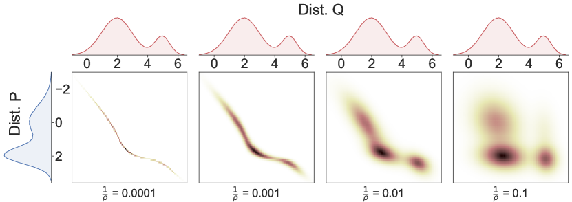
Figure 1. The coefficient $1/\rho$ in regularized OT impacts the mapping between distributions $P$ and $Q$: higher coefficients (on the right) lead to smoother mappings and spread mass more evenly between $P$ and $Q$.

Entropic Regularization:

OT problems, as described by Equation 2, essentially involve solving a linear program. The computational complexity of solving such a linear program $O(n^{3}\log n)$ using the network simplex, where $n$ represents the number of variables or constraints (Pele and Werman, 2009). This complexity can become a significant challenge, especially for high-dimensional datasets. To mitigate this computational burden, entropic regularization has been introduced as an effective strategy (Cuturi, 2013). By incorporating an entropy term into the optimal transport formulation, the problem is transformed into a nonlinear but smooth optimization problem, which can be solved more efficiently. This adjustment not only reduces the complexity of the problem but also enables its solution using linear-time algorithms. In the case of entropic regularization, the added entropy term effectively spreads out the transport plan, preventing the concentration of mass in a few narrow pathways. This spreading leads to a more evenly distributed plan, reducing the presence of sharp peaks and troughs in the optimization landscape. As a result, the optimization problem becomes more regular, with a smoother surface that is easier to navigate using optimization algorithms.

In more formal terms, the entropic OT is defined by:

(3) $$\operatorname*{argmin}_{\pi\in\Pi(P,Q)}\sum_{\textbf{x}_{i}\in\mathcal{X}}\sum_{\textbf{y}_{j}\in\mathcal{Y}}c(\textbf{x}_{i},\textbf{y}_{j})\pi(\textbf{x}_{i},\textbf{y}_{j})-\frac{1}{\rho}H(\pi).$$

where $H(\pi)$ is the entropic regularizer:

$$H(\pi)=-\sum_{\textbf{x}_{i}\in\mathcal{X}}\sum_{\textbf{y}_{j}\in\mathcal{Y}}\pi(\textbf{x}_{i},\textbf{y}_{j})\log(\pi(\textbf{x}_{i},\textbf{y}_{j}))$$

and $1/\rho$ is the entropic regularization parameter. A smaller value means that we emphasize the accuracy of the transport plan, while a larger value leans towards computational efficiency.

Importantly, the OT plan $\pi^{*}$, which solves the constrained optimization problem defined in (3), manifests as a diagonal scaling of the matrix $\textbf{K}\mathrel{\mathop{\ordinarycolon}}=e^{-\frac{\textbf{C}}{\rho}}$. Specifically, it has been shown that the solution to (3) is unique and takes the form $\pi^{*}=\text{diag}(\mathbf{u})\cdot\textbf{K}\cdot\text{diag}(\mathbf{v})$, with $\mathbf{u}$ and $\mathbf{v}$ acting as scaling vectors. These scaling vectors are identified through an iterative process, which ensures that the resultant transport plan complies with marginal probability constraints. The Sinkhorn Algorithm, crucial for this process, iteratively adjusts $\mathbf{u}$ and $\mathbf{v}$ to ensure that the resultant transport matrix, $\pi^{*}$, adheres to the given marginal constraints. Lines 4 and 5 of Algorithm 1 represent these adjustments. Specifically, u and v are updated iteratively to balance the rows and columns of K, ensuring that the marginals of the scaled coupling matrix $\pi$ closely match p and q.

Input: Probability distributions $P,Q$ and cost function $c$

Output: A transport plan between $P$ and $Q$

1 $\textbf{p}\mathrel{\mathop{\ordinarycolon}}=\textit{vector}(P);\textbf{q}\mathrel{\mathop{\ordinarycolon}}=\textit{vector}(Q);\textbf{C}\mathrel{\mathop{\ordinarycolon}}=\textit{matrix}(c);$

2 $\textbf{u}\mathrel{\mathop{\ordinarycolon}}=\mathbbm{1}_{d_{\mathcal{X}}};\textbf{v}\mathrel{\mathop{\ordinarycolon}}=\mathbbm{1}_{d_{\mathcal{Y}}};\textbf{K}\mathrel{\mathop{\ordinarycolon}}=e^{-\frac{\textbf{C}}{\rho}};$ $\triangleright$ Initialization

3 while u and v are not converged do $\triangleright$ Sinkhorn iterations

4       $\textbf{u}\mathrel{\mathop{\ordinarycolon}}=\textbf{p}\oslash(\textbf{K}\cdot\textbf{v});$ $\triangleright$ $\oslash$: Element-wise division

5       $\textbf{v}\mathrel{\mathop{\ordinarycolon}}=\textbf{q}\oslash(\textbf{K}\cdot\textbf{u});$

6      

7$\pi\mathrel{\mathop{\ordinarycolon}}=\textit{diag}(\textbf{u})\cdot\textbf{K}\cdot\textit{diag}(\textbf{v});$

return $\pi;$

Algorithm 1 Sinkhorn Algorithm

Example 2.1.

Figure 1 presents the optimal transport between two Gaussian mixture model distributions, $P$ and $Q$. Each distribution is a mixture of two Gaussians, providing a basis for examining the effects of entropic regularization on transport plans. The leftmost graph in Figure 1 shows the original OT plan without entropic regularization. The optimal plan is more deterministic and sharp in mapping elements between the distributions. As we introduce and increase the entropic regularization coefficient, the subsequent transport plans become more spread out. This spread is visually observable in Figure 1, where higher coefficients lead to transport plans that are less focused and more distributed across the space. This effect illustrates the principle of entropic regularization: a lower coefficient results in a transport plan that closely aligns specific elements of the distributions, whereas a higher coefficient allows for a broader, more generalized mapping. The intuition behind these transport plans can be understood by considering how the elements of one distribution, say ranging between $-2$ and $3$ in $P$, might be transported to another distribution $Q$ with values ranging between $0$ and $6$. Without regularization, the transport plan seeks to map these elements in a direct and specific manner. However, with entropic regularization, the mapping allows for the mass from one value in $P$ to be spread across the target distribution and to be transported to many values in $P$, thereby avoiding overly precise mappings that might not generalize well across different scenarios. This approach is particularly useful when dealing with high-dimensional data, where overly specific mappings can lead to overfitting and reduced model robustness.

Relaxed Optimal Transport:

Relaxed OT, introduced in (Frogner et al., 2015), provides a loss function for supervised learning grounded in OT principles. Rather than relying on hard marginal constraints typical of entropic regularized OT, it adopts softer penalties, using regularization based on the Kullback-Leibler (KL) divergence. This approach leads to:

$$\operatorname*{argmin}_{\pi\in\mathcal{J}}\sum_{\textbf{x}_{i}\in\mathcal{X}} \sum_{\textbf{y}_{j}\in\mathcal{Y}}c(\textbf{x}_{i},\textbf{y}_{j})\pi(\textbf{x}_{i},\textbf{y}_{j})-\frac{1}{\rho}H(\pi)\;+$$

(4) $$\lambda(D_{{\mathrm{KL}}}(\pi({Y}),Q)+D_{{\mathrm{KL}}}(\pi({X}),P)).$$

where $\lambda$ is the relaxation regularization coefficient, and $D_{{\mathrm{KL}}}$ denotes the KL divergence between two probability distributions. Contrasting this with the entropic OT outlined in Equation 3, the transport plan $\pi$ in relaxed OT can be an element of $\mathcal{J}$, which includes all possible joint probability distributions over the product space $\Delta_{{\mathbf{X}}}\times\Delta_{{\mathbf{Y}}}$. It has been shown in (Frogner et al., 2015) that Sinkhorn algorithm also works for the relaxed version of the entropic OT in Equation 3 but with different update rules for u and ${\mathbf{v}}$ (Frogner et al., 2015, Proposition 4.2):

(5) $$\textbf{u}=(\textbf{p}\oslash(\textbf{K}\cdot\textbf{v}))^{\frac{\rho\lambda}{\rho\lambda+1}}\hskip 14.22636pt\text{and}\hskip 14.22636pt\textbf{v}=(\textbf{q}\oslash(\textbf{K}^{\top}\cdot\textbf{u}))^{\frac{\rho\lambda}{\rho\lambda+1}}$$

3. Problem Definition

Given a database ${D}$ that is inconsistent with a CI constraint $\sigma\mathrel{\mathop{\ordinarycolon}}({\mathbf{X}}\mbox{$\perp\!\!\!\perp$}{\mathbf{Y}}\mid{\mathbf{Z}})$, our objective is to resolve this inconsistency by updating the attribute values of each datapoint in ${D}$ to derive a repaired database $\hat{{D}}$ which is consistent with $\sigma$. To ensure minimal distortion and maintain the utility of the data, we assume we are given a user-defined cost function that quantifies the cost of updating a datapoint (this cost function generalizes the minimality criteria in update-based data repair in databases (Bertossi, 2006)). Leveraging the principles of OT, our goal is to develop a data cleaner, envisioned as a transport map, that repairs ${D}$ at a minimum cost. Next, we define the problem of learning an optimal data cleaner for a CI constraint.

Definition 3.1 (CI Data Cleaner).

Consider a database ${D}=\{{\mathbf{v}}_{i}\}_{i=1}^{n}$ that violates a CI constraint $\sigma$, i.e., ${D}\not\models\sigma$, and a user-defined cost function $c\mathrel{\mathop{\ordinarycolon}}\mathcal{V}\times\mathcal{V}\rightarrow\mathbb{R}_{\geq 0}$ that assigns a cost to transforming or perturbing one tuple in $\mathcal{V}$ to another tuple in $\mathcal{V}$. The CI data cleaner of ${D}$ with respect to $\sigma$ is a transport map $T^{*}\mathrel{\mathop{\ordinarycolon}}\mathcal{V}\rightarrow\mathcal{V}$ that transforms ${D}$ into a database $\hat{{D}}=T^{*}({D})=\{\hat{{\mathbf{v}}_{i}}=T^{*}({\mathbf{v}}_{i})\}_{i=1}^{n}$ such that $\hat{{D}}\models\sigma$ and has the minimum transportation cost, i.e., $T^{*}$ is the solution to the following constrained optimization problem:

(6) $$\arg\min_{T}\sum_{i=1}^{n}c({\mathbf{v}}_{i},T({\mathbf{v}}_{i})) \text{s.t.}\quad T({D})\models\sigma.$$

We illustrate an optimal data cleaner with an example:

Example 3.2.

Let’s consider a database ${D}_{1}=\{(0,0,1)$, $(1,0,1)$, $(0,1,1)$, $(0,1,0)\}$ defined over binary variables $X$, $Y$, and $Z$. ${D}_{1}$ violates the CI constraint $\sigma\mathrel{\mathop{\ordinarycolon}}Y\mbox{$\perp\!\!\!\perp$}Z$ because the probability $P_{Y,Z}(1,0)$ is $\frac{1}{4}$, which is not equivalent to the product of the marginal probabilities $P_{Y}(1)=\frac{2}{4}$ and $P_{Z}(0)=\frac{1}{4}$. Further, suppose cost is measured using Euclidean distance. An optimal CI repair can be obtained using the transport map $T$, which maps $(0,0,1)\rightarrow(0,0,0)$ and other tuples to their current values. As a result, by updating one attribute value, $T$ transforms ${D}_{1}$ into a repaired database $\hat{{D}_{1}}=\{(0,0,0),(1,0,1),(1,1,0),(0,1,1)\}$, which is consistent with $\sigma$.

However, the CI data cleaner defined in Definition (3.1) might not lead to a minimum cost repair. This is especially true if ${D}$ is a bag, which is typically the case with databases used for ML. These databases are either bags or projections onto a subset of features that yield a bag. We illustrate this with an example:

Example 3.3.

Continuing with Example 3.2, now consider a database ${D}_{2}=\{(1,0,0),(1,0,1),(1,1,0),(1,1,0)\}$, which is now a bag, and is inconsistent with the constraint $Y\mbox{$\perp\!\!\!\perp$}Z$. Similarly, $\hat{{D}_{2}}=\{(1,0,0)$, $(1,0,1)$, $(1,1,0)$, $(1,1,1)\}$ is a minimum cost repair for ${D}_{2}$, obtained by modifying only one attribute value. However, no transport map exists that can transport ${D}_{2}$ into $\hat{{D}_{2}}$ simply because $(1,1,0)$ cannot be mapped to both itself and $(1,1,1)$. Upon close examination, it becomes evident that no transport map can lead to a repair for ${D}_{2}$ with cost 1.

Probabilistic Optimal Data Cleaner

As demonstrated in Example 3.3, the transport map defined in Definition 3.1 does not always yield the minimum cost repair (although it can always produce a trivial repair by mapping every tuple to a single tuple, which completely distorts the distribution). Indeed, it’s possible for the minimum cost repair to be outside the feasible region defined by the problem in Equation (6). Drawing from the Kantorovich relaxation of OT, we shift our approach to seeking a transport plan, or transport coupling, denoted as $\pi({\mathbf{v}}^{\prime},{\mathbf{v}})$, as an alternative to a deterministic transport map $T$. Here, the marginal distribution $\pi({\mathbf{v}})=P^{{D}}$ represents the empirical distribution of the database ${D}$, and $\pi({\mathbf{v}}^{\prime})$ is the target distribution that is consistent with the CI constraint. This transport plan yields a probabilistic mapping, $\pi({\mathbf{v}}^{\prime}\mid{\mathbf{v}})$, which probabilistically updates a data point ${\mathbf{v}}\in{D}$ to ${\mathbf{v}}^{\prime}$ following the mapping. The repaired database is then obtained by applying this mapping to ${D}$, by sampling. In essence, Definition 3.1 transitions into a problem where the aim is to (1) identify a transport plan $\pi({\mathbf{v}}^{\prime},{\mathbf{v}})$ that pushforwards the distribution $\pi({\mathbf{v}})=P^{{D}}$, i.e., the empirical distribution associated with ${D}$ into one consistent with the CI constraints, and (2) among all distributions with the same support and consistent with the constraint, find the distribution $\pi({\mathbf{v}}^{\prime})$ with the minimum OT distance to $\pi({\mathbf{v}})=P^{{D}}$. Formally, an optimal probabilistic data cleaner for CI constraint seeks to clean data using a probabilistic mapping $\pi(\mathbf{v}^{\prime}\mid\mathbf{v})$ associated with a transport plan or probabilistic coupling $\pi(\mathbf{v}^{\prime},\mathbf{v})$, obtained by solving the following optimization problem:

(7) $$\arg\min_{\pi}\sum_{i=1}^{d_{\mathcal{V}}}\sum_{j=1}^{d_{\mathcal{V}}}c(\mathbf{v}_{i},\mathbf{v}^{\prime}_{j})\pi(\mathbf{v}_{i},\mathbf{v}^{\prime}_{j}) \ \ \text{s.t.}\ \ \pi(\mathbf{v})=P^{\mathrm{{D}}},\;\pi({\mathbf{v}}^{\prime})\models\sigma.$$

The feasible region of the optimization problem defined in Equation 7 consists of all possible probability distributions that satisfy the constraint, hence including a distribution associated with a minimal cost repair. Therefore, one can find a mapping that transforms the empirical distribution of ${D}$ into a consistent distribution with the minimum cost. Moreover, the optimal probabilistic mapping, derived from solving Equation 7, provides an approach for probabilistic data cleaning. For large datasets, samples drawn from this probabilistic cleaner will lead to a dataset $\hat{{D}}$ whose empirical distribution $P^{\hat{{D}}}$ closely aligns with the target distribution $P(\mathbf{v^{\prime}})$, in line with the law of large numbers. Consequently, the resulting dataset is approximately consistent with the constraint. In ML applications, this level of approximation is generally adequate.

Figure 2. Graphical representation of the plan $\pi({\mathbf{v}},{\mathbf{v}}^{\prime})$ for ${D}_{2}$. Nodes represent elements in $\mathcal{V}$. Labeled red edges indicate joint probabilities $\pi({\mathbf{v}},{\mathbf{v}}^{\prime})$, while dashed directed edges depict the probabilistic mapping $\pi({\mathbf{v}}\mid{\mathbf{v}}^{\prime})$. Only nodes and edges with non-zero probabilities are shown for clarity.

Example 3.4.

Consider ${D}_{2}=\{(1,0,0)$, $(1,0,1)$, $(1,1,0)$, $(1,1,0)\}$ from Example 3.3. The probabilistic mapping $\pi({\mathbf{v}},{\mathbf{v}}^{\prime})$ is graphically represented in Figure 2, which depicts the bipartite graph constructed from the elements of the domain $\mathcal{V}$. Labeled red edges illustrate the joint probabilities $\pi({\mathbf{v}},{\mathbf{v}}^{\prime})$, while dashed directed edges showcase the corresponding probabilistic mapping $\pi({\mathbf{v}}\mid{\mathbf{v}}^{\prime})$. The graph only includes nodes and edges for which $\pi({\mathbf{v}},{\mathbf{v}}^{\prime})$ and $\pi({\mathbf{v}}\mid{\mathbf{v}}^{\prime})$ are non-zero to maintain clarity. It’s evident that the marginal distribution $\pi({\mathbf{v}})$ displayed in Figure 2 matches the empirical distribution $P^{{D}_{2}}$ associated to ${D}_{2}$. Furthermore, $\pi({\mathbf{v}}\mid{\mathbf{v}}^{\prime})$ primarily maps all elements to themselves with a probability of 1. However, it transports half of the mass from $(1,1,0)$ to itself and the other half to $(1,1,1)$ to repair the constraint violation. This results in a distribution $\pi({\mathbf{v}}^{\prime})$ consistent with the constraint. Notably, the OT cost of this repair is $1/4$ since just $1/4$ of the mass with cost 1 transitions from $(1,1,0)$ to $(1,1,1)$.

The mapping $\pi({\mathbf{v}}\mid{\mathbf{v}}^{\prime})$ can be employed to clean ${D}_{2}$ probabilistically. Due to the limited sample size, this doesn’t guarantee consistency. Still, for a larger database, the repaired database becomes representative of $\pi({\mathbf{v}}^{\prime})$ and hence becomes consistent with the constraint. To illustrate this, consider another database ${D}_{3}$ echoing the tuples in ${D}_{2}$, but each tuple is now replicated $n$ times. This mirrors the empirical distribution of ${D}_{2}$ and still violates the constraint. In such a scenario, repairing ${D}_{3}$ with $\pi({\mathbf{v}}\mid{\mathbf{v}}^{\prime})$ likely results in a consistent database. Probabilistically repairing the $2n$ instances of $(1,1,0)$ in ${D}_{3}$ through the mapping $\pi({\mathbf{v}}^{\prime}\mid{\mathbf{v}})$ can be interpreted as a sequence of $2n$ Bernoulli trials with a 1/2 probability. On average, this yields $n$ tuples of $(1,1,0)$ and $n$ tuples of $(1,1,1)$, ensuring consistency with the constraints.

Discussion on Complexity

Designing scalable algorithms to solve the optimization problem outlined in (7) and subsequently computing optimal repairs for CI constraints presents significant challenges. A straightforward approach entails exploring the vast space of all distributions consistent with the CI, computing OT distance in relation to the empirical distribution of ${D}$, and identifying the optimal solution. This method, however, is not feasible primarily due to the intractable nature of the space of consistent distributions. Furthermore, as discussed in 1, the computation of OT is computationally demanding. In our context, the transport plan involves $d_{\mathcal{V}}^{2}$ variables, thereby exacerbating the inherent complexity.

Although a detailed complexity analysis of the optimization problem 7 is not addressed in this paper, it is worth noting that our problem is akin to the computation of minimum update-based repair (U-repair) for MVDs (Bertossi, 2006). U-repair aims to identify a repair that necessitates the fewest attribute value modifications to enforce an MVD. Specifically, given a database $D$ with attributes $XYZ$ and an MVD $X\twoheadrightarrow Y$, the decision problem is whether $D$ has an optimal U-repair with no more than $k$ modifications. This decision problem can be translated to our repair challenge by presuming a uniform distribution over $D$, considering a cost function $c(x,y,z,x^{\prime},y^{\prime},z^{\prime})$ that enumerates the number of modifications required to obtain $(x^{\prime},y^{\prime},z^{\prime})$ from $(x,y,z)$, and checking if $D$ can achieve an optimal repair at a cost lesser than $k$ given the conditional independence $X\mbox{$\perp\!\!\!\perp$}Y\mid Z$. Under the specified assumptions, it is easy to check $D\models(X\mbox{$\perp\!\!\!\perp$}Y\mid Z)$ if and only if $D\models X\twoheadrightarrow Y$. While there’s extensive literature on the U-repair problem for Functional Dependencies (Kolahi and Lakshmanan, 2009; Livshits et al., 2020), to the best of our knowledge, it hasn’t been studied for MVDs.

4. Efficient Computation of Probabilistic Optimal Data Cleaner

In this section, we introduce efficient methods for computing the optimal data cleaner for CI constraints as described in (7). In Section 4.1, we formulate the problem as a Quadratically Constrained Linear Program (QCLP). This formulation allows for the derivation of an exact solution using existing efficient algorithms designed for QCLP. Subsequently, in Section 4.2, we present an approximate version of the optimization problem in (7). This approach facilitates the development of scalable and efficient solutions using iterative algorithms, particularly those based on Sinkhorn’s matrix scaling.

4.1. QCLP Formulation

We present a QCLP designed to find an optimal data cleaner, as outlined in Section 3. This program takes three inputs: a database $D$, a CI constraint $\sigma$, and a cost function $c$. We assume that $\sigma$ is a saturated CI constraint (i.e., it contains all attributes of $D$ cf. 9.3), with discussions on extending to unsaturated CI in Section 5.

To formulate the QCLP, we first describe the decision variables in the program, followed by an explanation of the constraints and the objective function. For clarity and better understanding, we use $D_{2}$ from Example 3.4 to demonstrate the QCLP formulation.

Figure 3. The QCLP for Example 4.1. The top left is the transport plan defined by the decision variables. The top right is $\tilde{Q}$ definitions. The rest are the objective and constraints.

Decision Variables

In the QCLP, decision variables are represented as $\tilde{\pi}_{i,j}$, where both $i$ and $j$ span from 1 up to $d_{\mathcal{V}}$ (reflecting the size of the support of ${\mathcal{V}}$). These variables are the transport plan’s probabilities representing the optimal data cleaning strategy. Since this plan has non-zero probabilities exclusively for the values present in $D$’s active domain, $i$’s range can be limited to the size of $D$’s active domain. The following example clarifies this.

Example 4.1.

In the QCLP for the optimal cleaner of $D_{2}$ from Example 3.4, the transport plan is defined by an $8\times 8$ variable matrix. However, given that $D_{2}$ contains only three records, we use a $3\times 8$ decision variable matrix, with the remaining rows of the initial matrix being zero. These decision variables indicate possible modifications to the three records in $D_{2}$, enabling them to align with any of the eight potential records in $\hat{D}_{2}$. The QCLP considers all eight potential records in $\hat{D}_{2}$, each associated with its distinct variable.

Constraints

The QCLP incorporates three types of constraints to encode the conditions in our data cleaner formulation in (7):

• Validity Constraints: These constraints, together with marginal constraints, ensure that $\tilde{\pi}$ makes a valid transport plan. Specifically, the decision variables must be non-negative real values:

  (8) $$\tilde{\pi}_{i,j}\geq 0\;\;\forall i\in[1,d_{\mathcal{V}}],j\in[1,d_{\mathcal{V}}]$$

• Marginal Constraints: These constraints are included to guarantee that the marginals of the transport plan, as described by $\tilde{\pi}$, align with $P^{D}$ (the empirical distribution of $D$):

  (9) $$\sum_{j=1}^{d_{\mathcal{V}}}\tilde{\pi}_{i,j}{\color[rgb]{0,0,0}=P^{D}(\textbf{v}_{i})}\;\;\;\forall i\in[1,d_{\mathcal{V}}]$$

• Independence Constraints: These constraints are formulated to ensure that the probability distribution $\pi(\textbf{v}^{\prime})$ satisfies the CI constraint $\sigma\mathrel{\mathop{\ordinarycolon}}(X\mbox{$\perp\!\!\!\perp$}Y\mid Z)$. To express these constraints, we introduce $\tilde{Q}$ as the marginal probability distribution obtained from the decision variables $\tilde{\pi}$. The independence constraints express the equation $\tilde{Q}_{X,Z}(x^{\prime},z^{\prime})\times\tilde{Q}_{Y,Z}(y^{\prime},z^{\prime})=\tilde{Q}(x^{\prime},y^{\prime},z^{\prime})\times\tilde{Q}_{Z}(z^{\prime})$ and guarantee the marginal probability distribution satisfies $\sigma$. We use the notation $\tilde{Q}$ instead of $Q$ to emphasize that the decision variables in $\tilde{\pi}$ specify the marginal probability distribution.

Objective

The objective of the QCLP is to minimize the transport cost, which is represented as follows:

(10) $$\min_{\tilde{\pi}}\sum_{i=1}^{d_{\mathcal{V}}}\sum_{j=1}^{d_{\mathcal{V}}}{c(\textbf{v}_{i},\textbf{v}j)\times}\tilde{\pi}_{i,j}$$

In this expression, the transport cost is calculated by summing the product of the cost function $c(\textbf{v}_{i},\textbf{v}j)$ and the decision variables $\tilde{\pi}_{i,j}$, over all elements in the set $\mathcal{V}$.

Example 4.2.

Expanding on Example 4.1, Figure 3 shows the constraints and objective present in the QCLP for $D_{2}$. Specifically, the validity constraints ensure that 24 decision variables are non-negative. The three marginal constraints verify the alignment of the marginal probability, as defined by the transport plan, with the probabilities of the three input records in $D_{2}$. The independence constraints ensure that the probability distribution specified by $\tilde{Q}$ satisfies $\sigma\mathrel{\mathop{\ordinarycolon}}X\mbox{$\perp\!\!\!\perp$}Y\mid Z$. For example, four independence constraints in this example guarantee $\sigma\mathrel{\mathop{\ordinarycolon}}Y\mbox{$\perp\!\!\!\perp$}Z$ holds for all possible values of $Y$ and $Z$. The first independence constraint is $\tilde{Q}_{Y,Z}(0,0)=\tilde{Q}_{Y}(0)\times\tilde{Q}_{Z}(0)$, where the marginals $\tilde{Q}_{Y,Z}(0,0),\tilde{Q}_{Y}(0)$, and $\tilde{Q}_{Z}(0)$ are defined as sums of decision variables in $\tilde{\pi}$. The costs in the objective are the Euclidean distance between the input records and their possible repair, e.g., the cost 1 in ${\color[rgb]{.75,0,.25}1\times}\tilde{\pi}_{1,1}$ is the Euclidean distance between $(1,0,0)$, as the first record in $D_{2}$, and $(0,0,0)$, as the first possible repair. Similarly 2 in ${\color[rgb]{.75,0,.25}2\times}\tilde{\pi}_{1,2}$ reflects the Euclidean distance between $(1,0,0)$ and $(0,0,1)$.

The above program is classified as a QCLP because, while the objective function and the validity and marginal constraints are linear with respect to the decision variables, the independence constraints are non-linear (quadratic). This is due to each side of the constraint consisting of a product of values in $\tilde{Q}$, that each is, in turn, a sum of the variables in $\tilde{\pi}$. QCLP represents a distinct subtype of Quadratically Constrained Quadratic Programs (QCQPs) or Second-Order Cone Programs (SOCPs) that feature quadratic constraints and objectives. Addressing a QCLP is a non-convex optimization problem and is NP-hard (Van de Panne, 1966; Boyd et al., 2004). Diverse, efficient methodologies, including sequential quadratic programming, augmented Lagrangian, interior-point, and active set, have been employed to derive sub-optimal solutions for such programs (Boyd et al., 2004).

We implemented an alternating algorithm to compute the optimal repair by solving the QCLP program. This method iteratively transforms the quadratic independence constraints into linear ones, similar to the Alternating Direction Method of Multipliers (ADMM) (Boyd et al., 2011). The process begins with initial variable estimates for $\tilde{\pi}$, ensuring the marginal distribution $\tilde{Q}$ satisfies $\sigma$. These initial values can be derived from the marginal probabilities of $P^{D}$. In each iteration, we partition the variables in $\tilde{\pi}$ into two subsets. We substitute the variables with their current estimates for the first subset, effectively linearizing the constraints. This transformation allows us to treat the second subset as variables within a linear program. In subsequent iterations, we alternate roles: treating variables of the second subset as constants and updating the first subset’s values by solving a distinct linear program. This alternating process continues until the variables stabilize, indicating convergence. We have omitted the algorithm’s specifics for brevity. The algorithm’s convergence proof is similar to that of ADMM as presented in (Boyd et al., 2011).

4.1.1. Analysis of the QCLP Solution

The QCLP formulation, though convergent, encounters scalability challenges. Specifically, in each iteration, it necessitates solving an OT problem which is structured as a linear program. The computational complexity of determining the OT scales as $O(d^{3}\log(d))$ when comparing histograms of dimension $d$ (Pele and Werman, 2009). In the following section, we introduce an alternative formulation that mitigates this scalability issue and obviates the need for solving a linear program.

4.2. Fast Approximation via Relaxed OT using Sinkhorn Iterations

In this section, we present an approximate algorithm for computing optimal repairs by casting the problem into a regularized optimization. This approach integrates the CI constraint and the constraint on marginals as regularizers, drawing inspiration from the relaxed optimal transport discussed in Section 9.3. Specifically, we formulate the problem of computing the optimal cleaner in (7) as the following regularized optimization problem:

$$\operatorname*{argmin}_{\pi\in\Pi,Q\in\Delta_{{\mathbf{V}}}} \sum_{\textbf{v}_{i}\in\mathcal{V}}\sum_{\textbf{v}^{\prime}_{j}\in\mathcal{V}}c(\textbf{v}_{i},\textbf{v}^{\prime}_{j})\pi(\textbf{v}_{i},\textbf{v}^{\prime}_{j})-\frac{1}{\rho}H(\pi)\;+$$

(11) $$\lambda(D_{{\mathrm{KL}}}(\pi({\mathbf{v}}^{\prime}),Q)+D_{{\mathrm{KL}}}(\pi({\mathbf{v}}),P^{D}))+\mu\;\delta_{\sigma}(Q),$$

In the above formulation, $P^{D}$ denotes the empirical distribution of the dataset $D$. The target distribution, represented by $Q$, functions as a decision variable, while $\pi$ is the transport plan. The regularization term $D_{{\mathrm{KL}}}(\pi({\mathbf{v}}^{\prime}),Q)+D_{{\mathrm{KL}}}(\pi({\mathbf{v}}),P^{D})$ penalizes the objective when there are deviations of its marginals $\pi({\mathbf{v}})$ and $\pi({\mathbf{v}}^{\prime})$ from $P^{D}$ and $Q$, respectively. Additionally, the CI constraint, represented by $\sigma$, is imposed on $Q$ through the regularization term $\delta_{\sigma}(Q)$ within the objective (recall from Section 1 that $\delta_{\sigma}(Q)=D_{{\mathrm{KL}}}[Q(X,Y,Z)\mid Q(X,Z)Q(Y\mid Z)]$). This term measures the degree of inconsistency of $Q$ in relation to $\sigma$ by utilizing the conditional mutual information, as discussed in Section 9.3. This method is in contrast from the hard constraints used in the QCLP formulation Section 4.1. The hyperparameters $\lambda$ and $\mu$ serve as regularization coefficients, adjusting for discrepancies from the marginals and the degree of inconsistency in the target distribution $Q$. The methodology for tuning these hyperparameters is discussed in Section 6.

Intuitively, the optimization problem aims to find a distribution $Q$ that aligns closely with the empirical distribution $P^{D}$ while being consistent with the imposed constraint. The relaxed OT distance serves as a measure of this alignment, and the objective is to minimize this distance, ensuring that $Q$ is a faithful representation of $P^{D}$ that simultaneously satisfies the constraint.

The inclusion of the CI constraint term makes our new formulation non-convex. We address this non-convexity with an alternating algorithm, FastOTClean. Before we detail FastOTClean in Algorithm 2, we describe its main idea. In this algorithm, we sequentially focus on either the transport plan $\pi$ or the resulting distribution $Q$, optimizing one while holding the other constant. Initially, we can set $Q$ to a distribution that meets the CI constraint $\sigma$. With this fixed value, our objective becomes a convex function, which we solve using the Sinkhorn matrix scaling algorithm discussed in Section 9.3. When we alternate, our goal becomes minimizing the divergence between $Q$ and $\pi({\mathbf{v}}^{\prime})$. In this stage, $Q$ must also align with the CI constraint $\sigma$.

To address this problem, we adopt an alternating minimization strategy. Initiating with an initial guess for $Q$, the algorithm first determines the optimal transport plan $\pi({\mathbf{v}},{\mathbf{v}}^{\prime})$ between $P^{D}$ and $Q$ through Sinkhorn iterations. In the subsequent iteration, a new $Q$ is constructed based on the target distribution of $\pi$, denoted $\pi({\mathbf{v}}^{\prime})$. Specifically, this $Q$ is identified to be proximate to $\pi({\mathbf{v}}^{\prime})$ based on the KL divergence while also ensuring it either approximately or strictly satisfies the independence constraint. In subsequent iterations, the transport plan is recalibrated with respect to the revised $Q$. Hence, the procedure can be viewed as a two-layered iterative process where the outer loop identifies a relaxed OT map, and the inner loop refines the target distribution of this map to enforce the constraint. The core intuition behind this approach is twofold. Firstly, the outer loop endeavors to determine a transport plan that maps the empirical distribution of data to a target distribution proximate to $Q$, influenced by the regularization coefficient; its primary objective is to minimize the transport cost. Conversely, the inner loop evaluates the target distribution derived from the outer mapping and formulates a distribution in close alignment with it, ensuring adherence to the constraint. In essence, while the outer loop emphasizes on minimizing the transportation cost, the inner loop focuses on enforcing independence constraints.

The inner loop of this alternating algorithm, which reconstructs $Q$ based on $\pi({\mathbf{v}}^{\prime})$ to satisfy the CI constraint, can be interpreted as a rank-one non-negative matrix factorization (as highlighted in Capuchin (Salimi et al., 2019)). Specifically, when dealing with conditional mutual information, the problem aligns with non-negative matrix factorization using the KL divergence objective, which is inherently non-convex but is typically addressed using alternating algorithms (for approximate enforcement of a CI constraint, one can use approximate matrix factorization techniques (Finesso and Spreij, 2004)). For a specific value $z\in{\mathcal{Z}}$, we aim to determine matrices $\mathbf{W}_{z}$ of size $d_{X}\times 1$ and $\mathbf{H}_{z}$ of size $d_{Y}\times 1$. These matrices represent the joint and conditional distributions $Q(X^{\prime},Z^{\prime}=z)$ and $Q(Y^{\prime}\mid Z^{\prime}=z)$. They are chosen to minimize the divergence $D_{{\mathrm{KL}}}(\pi(X^{\prime},Y^{\prime},Z^{\prime}=z)\mid\mathbf{W}_{z}\cdot\mathbf{H}_{z}^{T})$. While the $D_{{\mathrm{KL}}}$ is convex with respect to either ${\mathbf{W}}_{z}$ or ${\mathbf{H}}_{z}$, it is not jointly convex for the pair $({\mathbf{W}}_{z},{\mathbf{H}}_{z})$. Established alternating methods, along with their associated update rules from the matrix factorization domain, such as those highlighted by Lee (Lee and Seung, 2000), can be employed. Starting with a random setup, these methods update $\mathbf{W}_{z}$ and $\mathbf{H}_{z}$ until they converge. The final matrices help us shape a new $Q$ that satisfies the independence constraint.

We outline the algorithm to solve the optimization problem in (11), denoted by FastOTClean, in Algorithm 2. It begins by setting initial values for the vectors p, q, and the cost matrix C (see Lines 2 to 2). The vector q is set up to represent probabilities in a distribution satisfying $\sigma$, which serves as a first guess for the resulting distributions $Q$. The vectors u and v, and the matrix K are then prepared for Sinkhorn iterations (Line 2). The Sinkhorn method find a plan $\pi$ between our original p and the estimate q by updating u and v until they stabilize (Line 2). See Section 9.3 on checking convergence. After this, the algorithm computes the transport plan $\pi$ (Line 2) and shifts its focus to reconstructing q. The reconstruction step (Line 2) employed an alternating algorithm as described before to update q.

Input: Database $D$, cost function $c$, and CI constraint $\sigma\mathrel{\mathop{\ordinarycolon}}X\mbox{$\perp\!\!\!\perp$}Y\mid Z$

Output: Transport plan (probabilistic data cleaner) $\pi$

1 $\textbf{p}\mathrel{\mathop{\ordinarycolon}}=\textit{vector}(P^{D});$ $\textbf{C}\mathrel{\mathop{\ordinarycolon}}=\textit{matrix}(c);$

2

3Randomly initialize q $\triangleright$ An initial guess for $Q$

4 $\textbf{u}\mathrel{\mathop{\ordinarycolon}}=\mathbbm{1}_{d_{\mathcal{X}}};\textbf{v}\mathrel{\mathop{\ordinarycolon}}=\mathbbm{1}_{d_{\mathcal{Y}}};\textbf{K}\mathrel{\mathop{\ordinarycolon}}=e^{-\frac{\textbf{C}}{\rho}};$ $\triangleright$ Sinkhorn Initialization

5 while q is not converged do $\triangleright$ Sinkhorn iterations

6      

7      while u and v are not converged do

8             $\textbf{u}\mathrel{\mathop{\ordinarycolon}}=(\textbf{p}\oslash(\textbf{K}\cdot\textbf{v}))^{\frac{\rho\lambda}{\rho\lambda+1}},\textbf{v}\mathrel{\mathop{\ordinarycolon}}=(\textbf{q}\oslash(\textbf{K}\cdot\textbf{u}))^{\frac{\rho\lambda}{\rho\lambda+1}};$

9      $\pi=\textit{diag}(\textbf{u})\cdot\textbf{K}\cdot\textit{diag}(\textbf{v});$

10       for each $z\in{\mathcal{Z}}$ do

11             Initialize ${\mathbf{W}}_{z}$, ${\mathbf{H}}_{z}$ randomly.

12             while  ${\mathbf{W}}_{z}$ and ${\mathbf{H}}_{z}$ are not converged do

13                   Update ${\mathbf{W}}_{z}$ to minimize $D_{{\mathrm{KL}}}(\pi(X^{\prime},Y^{\prime},Z^{\prime}=z)\mid\mathbf{W}_{z}\cdot\mathbf{H}_{z}^{T})$ with ${\mathbf{H}}_{z}$ fixed

14                   Update ${\mathbf{H}}_{z}$ to minimize $D_{{\mathrm{KL}}}(\pi(X^{\prime},Y^{\prime},Z^{\prime}=z)\mid\mathbf{W}_{z}\cdot\mathbf{H}_{z}^{T})$ with ${\mathbf{W}}_{z}$ fixed

15            

16      Construct q using ${\mathbf{W}}_{z}$s and ${\mathbf{H}}_{z}$s computed in the previous step

return $\pi$;

Algorithm 2 FastOTClean: Fast Computation of Probabilistic Data Cleaner for Conditional Independence

4.2.1. Analysis of the algorithm

We prove that the algorithm converges. In Section 6, we empirically demonstrate the inner workings and convergence properties of this algorithm. In Section 5, we propose efficient strategies to further optimize this algorithm.

Theorem 4.3.

For the optimization problem outlined in Equation (11), Algorithm 2 converges.

Proof.

Algorithm 2 can be understood as an iterative optimization over one variable, either the transport plan $\pi$ or the distribution $Q$, while holding the other variable constant. When $Q$ is fixed, optimization concerning the transport plan is smooth, differentiable, and strictly convex, ensuring that the Sinkhorn iterations converge, as established by (Frogner et al., 2015). Conversely, with a fixed $\pi$, the inner problem breaks down into an objective function that remains strictly convex with respect to each matrix separately, and the adopted update rule ensures convergence to a stationary point, as elaborated in (Hien and Gillis, 2021). This approach mirrors the Coordinate Descent method, where the objective function is convex for each individual coordinate. As per (Tseng, 2001)[theorem 5.1], this process guarantees convergence to a coordinate-wise minimum of the objective function. ∎

5. Optimizations

We applied several optimizations to improve FastOTClean that we briefly explain below and show their efficacy in Section 6.

Default Optimization

We applied two straightforward yet effective optimizations: 1) Confining the transport plan’s size to restrict mass movement solely within $D$’s active domain to $\mathcal{V}$, excluding movement to the entire support. We explained this in the context of QCLP while defining decision variables in Section 4.1. This restriction can be further narrowed down to allow mass movement within a more limited subset. 2) Rather than randomly initializing the target distribution $Q$ in FastOTClean, we initiated it with a distribution satisfying the CI constraint by applying Non-negative Matrix Factorization (NMF) to the empirical distribution of $D$, which our results demonstrated to aid faster convergence.

Warm Starting Sinkhorn

Convergence of the Sinkhorn iteration is a significant bottleneck in FastOTClean. We observe that our alternating algorithm, while it changes $Q$ in each iteration in which we fix the transport plan, only makes slight adjustments, implying that the transport plan should undergo minor changes in the next iteration. Therefore, instead of initializing the Sinkhorn scaling factors ${\mathbf{u}}$ and ${\mathbf{v}}$ with vectors of ones, adopting a warm starting approach by initializing them with the ${\mathbf{u}}$ and ${\mathbf{v}}$ from the previous iteration can significantly accelerate convergence. Our evaluation results indicate that this is a highly effective idea.

Unsaturated CI Constraints

So far, we assumed that $\sigma\mathrel{\mathop{\ordinarycolon}}X\mbox{$\perp\!\!\!\perp$}Y\mid Z$ represents a saturated CI constraint, implying ${\mathbf{V}}=\{X,Y,Z\}$. However, in many real-world scenarios, especially with high dimensional data, CI constraints may not be saturated.

For unsaturated constraints, we split ${\mathbf{V}}$, the set of attributes in the database $D$, into two sets: ${\mathbf{U}}=\{X,Y,Z\}$ (the attributes in $\sigma$) and ${\mathbf{W}}={\mathbf{V}}\setminus{\mathbf{U}}$ (those not in $\sigma$). A naive method is to compute a transport plan $\pi$ of size $d^{2}_{\mathcal{V}}$, considering all attributes in ${\mathbf{V}}$, including ${\mathbf{W}}$. Adapting methods from Section 4 for this scenario is straightforward but computationally expensive with high-dimensional data.

A more efficient strategy is to run FastOTClean for the marginal distribution $P^{D}_{\mathbf{U}}$ instead of $P^{D}$. This results in a smaller transport plan $\pi_{s}$ of size $d^{2}_{\mathcal{U}}$ compared to $\pi$. With $\pi_{s}$, we construct $\pi$ as follows: $\pi(\textbf{v},\textbf{v}^{\prime})=0$ if $\textbf{w}\neq\textbf{w}^{\prime}$, and $\pi(\textbf{v},\textbf{v}^{\prime})=\pi_{s}(\textbf{u},\textbf{u}^{\prime})P_{{\mathbf{W}}\mid{\mathbf{U}}}(\textbf{w}\mid\textbf{u})$ otherwise. This ensures no additional transport cost for moving masses between different values of ${\mathbf{W}}$ as there is no mass moved for $\textbf{w}\neq\textbf{w}^{\prime}$. Thus, the cost associated with $\pi$ is the same as $\pi_{s}$, making it optimal if $\pi_{s}$ is optimal. Note that this requires the cost function to satisfy some basic properties, such as the cost of $\textbf{u}\textbf{w}\rightarrow\textbf{u}^{\prime}\textbf{w}$ being equal to the cost of $\textbf{u}\rightarrow\textbf{u}^{\prime}$, which is satisfied by the Euclidean distance and other cost functions in our work. Additionally, the use of $P_{{\mathbf{W}}\mid{\mathbf{U}}}(\textbf{w}\mid\textbf{u})$ ensures that $\pi$ satisfies the marginal constraint $P^{D}(\textbf{v})=\pi(\textbf{v})$. The resulting distribution $Q$ from $\pi$ satisfies $\sigma$ as its marginal is $Q_{{\mathbf{U}}}$ which is known to satisfy $\sigma$.

6. EXPERIMENTS

In our experimental evaluation of OTClean, we seek to answer the following research questions: Q1 How does the end-to-end performance of OTClean in terms of algorithmic fairness compare with baseline approaches? (Section 6.2) Q2 In data cleaning tasks related to CIs, how does the performance of OTClean compare with the baselines? (Section 6.3) Q3 How effective is OTClean in determining optimal repairs? This encompasses evaluating its convergence behavior, runtime performance, and efficacy of the optimizations. (Section 6.5)

Dataset	#tuples	#attr.	avg. dom	init. CMI
Adult	48,842	14	5.42	0.18770
COMPAS	10,000	12	2.4	0.05484
Car	1,728	6	3.67	0.03617
Boston	506	14	4.5	0.05983

Table 2. Datasets characteristics

Datasets

We used four datasets. The Adult and COMPAS datasets highlight the fairness aspect of OTClean’s application, while the datasets Car and Boston showcase the efficacy of OTClean in data cleaning tasks. Table 2 provides an overview of these datasets.

Adult (adu, 2023)

In the Adult dataset, or “Census Income,”, each entry captures details like age, work class, education level, marital status, occupation, relationship status, race, gender, weekly working hours, and country of origin. The dataset’s main objective is to predict if an individual earns over $50K annually.

COMPAS (com, 2023)

The COMPAS dataset from the Broward County Sheriff’s Office in Florida predicts the likelihood of an individual re-offending. Key attributes include age, gender, race, criminal history, risk scores, charge degree, and jail history. COMPAS is essential for studies focusing on the fairness implications of predictive policing.

Car (car, 2023)

The Car Evaluation dataset evaluates cars based on attributes like buying price, maintenance cost, number of doors, person capacity, and safety. Cars are classified based on their overall condition into unacceptable, acceptable, good, or very good.

Boston (bos, 2023)

The Boston Housing dataset provides insights into the housing market in Boston, Massachusetts. It covers attributes like crime rate, residential zoning, average room count, distance to employment centers, and median home value. It’s frequently used for regression analysis in predicting housing prices.

Baselines

We use baselines that we briefly review here.

Algorithmic fairness

In the realm of algorithmic fairness, the objective is to guarantee that decision-making algorithms operate equitably, avoiding discrimination based on sensitive attributes like race or gender. While there are myriad definitions of fairness in the literature, this study primarily focuses on interventional fairness, as articulated in (Salimi et al., 2019). This particular notion underscores the importance of enforcing conditional independence within data. Consider a sensitive attribute $S$. Without loss of generality, let’s assume $S$ is binary where $S=1$ denotes the protected (or sensitive) group and $S=0$ the unprotected group. Further, consider a ML model with output $\hat{Y}$ trained on a set of features ${\mathbf{X}}$. The notion of interventional fairness divides ${\mathbf{X}}$ into two sets: admissible variables ${\mathbf{A}}$ and inadmissible variables ${\mathbf{N}}$. Admissible variables are those where the effect of the sensitive attribute on the outcome, mediated by these variables, is considered fair. In (Salimi et al., 2019), the extent to which a ML model deviates from this fairness standard is quantified using the Ratio of Observational Discrimination (ROD), defined as:

$$\text{ROD}=\frac{1}{|dom(A)|}\sum_{a\in A}\frac{P(\hat{Y}=1|S=0,a)P(\hat{Y}=0|S=1,a)}{P(\hat{Y}=0|S=0,a)P(\hat{Y}=1|S=1,a)}$$

A ROD value of 1 signals the absence of any bias and is in correspondence to the conditional independence $(\hat{Y}\mbox{$\perp\!\!\!\perp$}S\mid{\mathbf{A}})$. In this paper, we employ the logarithm of the ROD for our analyses. A logarithmic ROD value of 0 is indicative of the absence of discrimination, while progressively higher values of the log ROD signify increasing levels of bias. The approach detailed in (Salimi et al., 2019) reduces the challenge of training a fair ML model to the task of enforcing a CI constraint on the training data. They introduced several methods in this context, which we adopt as baselines for our evaluations. Their methods fall into two categories: Methods based on matrix factorization and MaxSat methods. From the first category, the “Cap(MF)” factorizes each joint probability distribution of $P^{D}$ for a fixed value of ${\mathbf{Z}}$ by minimizing Euclidean norm, while “Cap(IC)” does the factorization by using marginals of the initial distribution. They also propose a problem reduction of repairing w.r.t a CI constraint to solving a general CNF formula, and they solve it using their MaxSat method “Cap(MS)”. We also included a naive baseline referred to as ’Dropped,’ where the model is trained solely on admissible variables, which is sufficient for enforcing intervention fairness, as demonstrated in (Salimi et al., 2019).

Data Cleaning

In our data cleaning evaluation, we assess the performance of OTClean and compare it with various imputation and data cleaning methods. We consider five baselines for handling missing values: 1) Most frequent (MF) fills missing values with the most frequent values within the attribute, 2) k-nearest neighbors (kNN) identifies the most frequent values among neighboring data points for imputation, 3) GAIN uses Generative Adversarial Networks (Yoon et al., 2018), and 4) Hyperimputation is a method that integrates multiple imputation techniques, blending traditional iterative imputation with deep learning (Jarrett et al., 2022). We selected kNN and MF as basic, widely-used baselines. We compared OTClean with GAIN since it is a leading imputation method and Hyperimpute since it is known for its ability to surpass various imputation techniques. We also use two baselines in scenarios with attribute noise: 1) using the dirty dataset as a simple baseline, and 2) Baran (Mahdavi and Abedjan, 2020) as an advanced data cleaning method that utilizes comprehensive context information, including the value, co-occurring values, and attribute type, to generate correction candidates with high precision.

6.1. Tuning OTClean

Cost function

We employ two cost functions in our experiments. The first function calculates the cost as the Euclidean distance between two records after normalizing their attributes by dividing them by their standard deviation. The second function utilizes a distance learned through MLKR (Metric Learning for Kernel Regression (Weinberger and Tesauro, 2007)), a supervised metric learning technique that minimizes the leave-one-out regression error. We chose MLKR because it is widely used for distance learning and designed explicitly for supervised tasks like those in our settings. We label the results from the first cost function as OTClean-C1, while the cost function using the learned distance is labeled as OTClean-C2.

Regularization Coeffients

Two tuning parameters of FastOTClean are $\lambda$ and $\frac{1}{\rho}$. As $\lambda$ and $\rho$ grow, our formulation of OTClean gets closer to the OT distance, and FastOTClean gives better results. However, as their values grow, the cost of running FastOTClean increases due to slower convergence. To find parameter values that balance runtime and fast convergence, we perform a grid search for each dataset to tune OTClean. OTClean has another parameter, $\mu$, that quantifies the dissatisfaction of the CI constraint.

6.2. Algorithmic Fairness

We evaluate the effectiveness of OTClean within the domain of algorithmic fairness. To harness OTClean for training interventionally fair algorithms, we utilize our probabilistic data cleaning approach to modify the data, ensuring its consistency with the CI constraint ($S\mbox{$\perp\!\!\!\perp$}{\mathbf{N}}\mid{\mathbf{A}}$). This enforced independence ensures the sensitive attribute does not influence the inadmissible variable, except through ${\mathbf{A}}$. If this independence is maintained, any valuable predictive information encapsulated within the inadmissible variables ${\mathbf{N}}$ cannot be sourced from the sensitive attribute. The flexibility of our approach, underpinned by optimal transport, allows us to craft specific cost functions for probabilistic data cleaning to preserve as much predictive capability as possible. Specifically, we designed a cost function to modify the inadmissible variables and keep sensitive attributes and admissible variables unchanged, ensuring that while fairness is achieved, all relevant predictive information within ${\mathbf{A}}$ is retained. Additionally, it ensures that any remaining predictive value within ${\mathbf{N}}$ is not derived from the sensitive attribute $S$.

We applied OTClean to establish a probabilistic data cleaner for the training data. This cleaner was subsequently used to pre-process the dataset. The subsequent sections present evaluation results on the Adult and COMPAS datasets. Our evaluation metrics include cross-validated AUC and the mean ROD averaged over iterations derived from cross-validation outcomes. Besides ROD, we also assess other fairness measures, such as equality of odds and demographic parity. Notably, our approach incidentally enhances these fairness metrics as well. We also report other popular fairness measures, such as equality of odds— which requires that classifiers have equal false positive and false negative rates across protected groups—and demographic parity, which ensures that the decision outcome is independent of the protected attribute.

Figure 4 showcases our evaluation results for the COMPAS and Adult datasets. In the Adult dataset, the sensitive attribute is “sex”, “marital-status” is inadmissible, and the admissible attributes include “occupation”, “education-num”, “hours-per-week”, and “age”. For COMPAS, we treat “race” as sensitive, “age-cat” and “priors-count” as inadmissible, and “charge-degree” as admissible. Notably, OTClean demonstrates superiority over the baseline, achieving models that are at least as fair, if not fairer, and exhibit an elevated AUC. This improvement can be attributed to our optimal transport-based approach, which empowers our method to retain considerable predictive value while rigorously enforcing fairness constraints. Furthermore, Figure 5 shows OTClean’s reasonable performance on other fairness notions, specifically Equality of Opportunity (EO) and Demographic Parity (DP). On both datasets, our methodology consistently surpasses the baseline in these respects. (Note: the result of “Cap(MS)” is not plotted in Figure 4(b) as it achieved a constant AUC of 0.5 in all cross-validation iterations.)

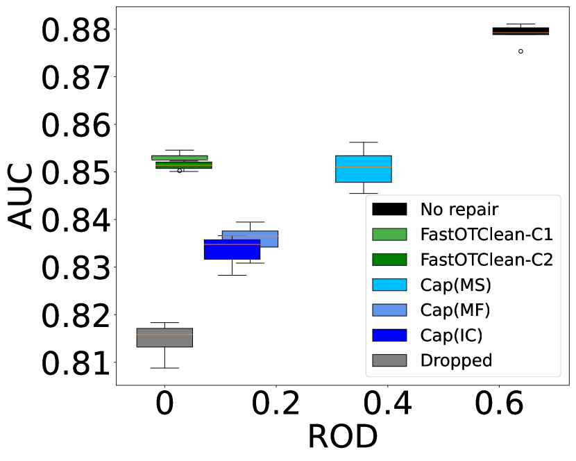
(a) Adult

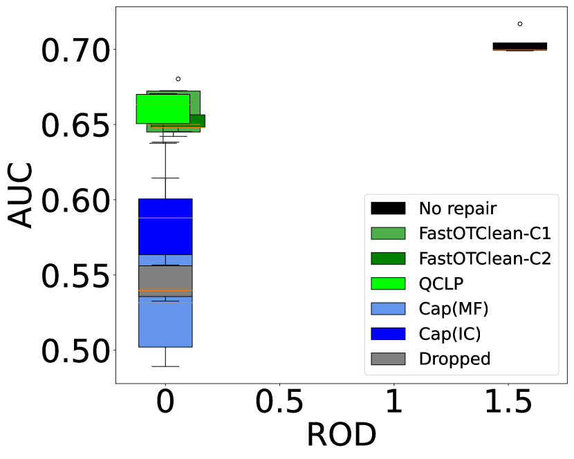
(b) COMPAS

Figure 4. Comparison of OTClean’s performance with the baselines showing higher AUC and lower ROD (bias)

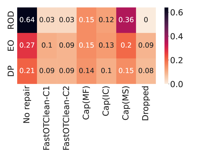
(a) Adult

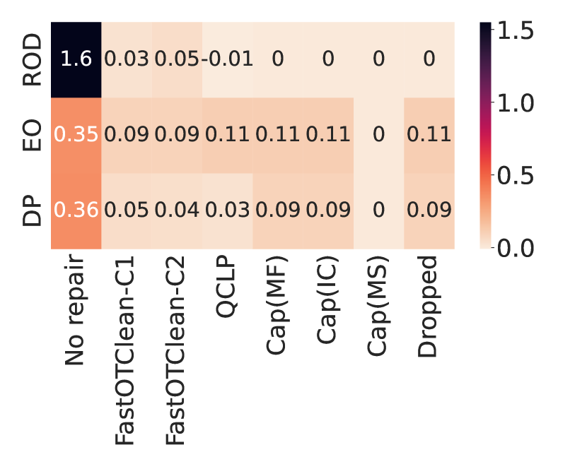
(b) COMPAS

Figure 5. Fairness metrics in OTClean, indicating lower biases (ROD, EO, and DP) compared to baseline methods

6.3. Data Cleaning

To evaluate the performance of OTClean in data cleaning, we conducted experiments using semi-synthetic datasets that featured two types of dirty data: attribute noise and missing values. These datasets were derived from the Car and Boston datasets. We used these datasets to train ML models for predicting the labels “class” (indicating the car’s condition in the Car dataset) and “medv” (representing median house price in the Boston dataset), respectively. In each case, we introduced noise errors and missing values into the training data, while the original clean data served as the test set for assessing model generalization. For Car, we considered the CI constraint ($\text{doors}\mbox{$\perp\!\!\!\perp$}\text{class}\,|\,\text{the remaining attributes}$). This constraint implies that the number of car doors should not significantly impact the class label when considering other factors such as buying price and safety. For the Boston dataset, we examined the constraint ($\text{B}\mbox{$\perp\!\!\!\perp$}\text{medv}\,|\,\text{the remaining attributes}$), which suggests that the “B” attribute (indicating the percentage of blacks per town) should not influence the “medv” label. Initially, these constraints approximately held in the original datasets. To introduce attribute noise, we deliberately added non-random noise that led to violations of the CI constraints. Additionally, we injected two types of missingness: missing at random (MAR) and missing not at random (MNAR).

We chose to use a semi-synthetic dataset, where we added errors to real-world data, to create both “dirty” datasets and their accurate ground truths. This was essential because it is difficult to find real datasets with both genuine errors and ground truth. A limitation of this approach is that the injected error patterns may not exactly replicate those in actual datasets. However, our cleaning system is designed to be effective regardless of the specific error types. It primarily targets fixing spurious correlations and reducing the impact of any differences in error patterns on our goals.

To create a dependency between two attributes through attribute noise, we introduce random noise into one based on the values of the other. For adding missing data, our approach depends on the type. In MAR scenarios, where an attribute’s missingness is influenced by another attribute, we decide to add missing values based on the other attribute’s values in the same record. In MNAR cases, where an attribute’s missingness is affected by its own value and other attributes, we randomly select records and determine missingness based on these factors. This method systematically creates relationships between attributes, effectively incorporating noise and addressing different missing data situations.

To assess the efficacy of OTClean, we utilized the “Dirty” datasets to train various ML models, including logistic regression, random forest, SVM, and MLP, and reported results for the best-performing model. When dealing with missing values, we employed two imputation methods: most frequent values (MF) and kNN, as explained previously. The dirty model is labeled with the imputation method used for training the dataset. In all experiments, the models were tested on ground truth data (the data before adding noise or missing values), and the models trained on the ground truth were denoted as “Clean.” Additionally, we applied OTClean to enforce the corresponding CI constraint before training the ML models. This step aimed to remove spurious correlations induced by violations of CI, which could lead to poor performance of the ML model.

(a) Car

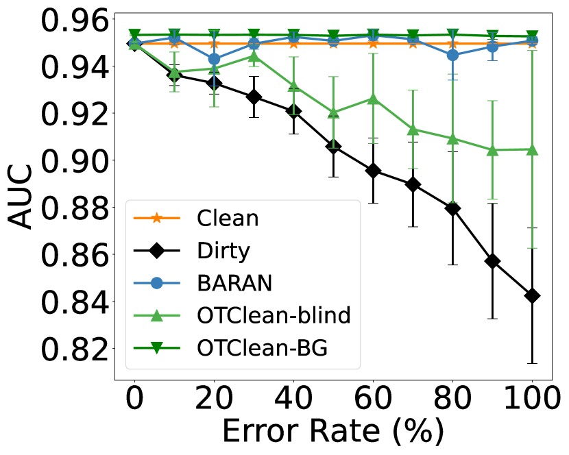
(b) Boston

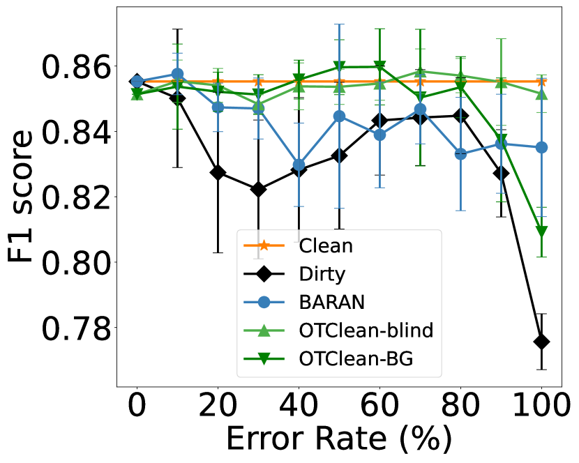
(c) Car

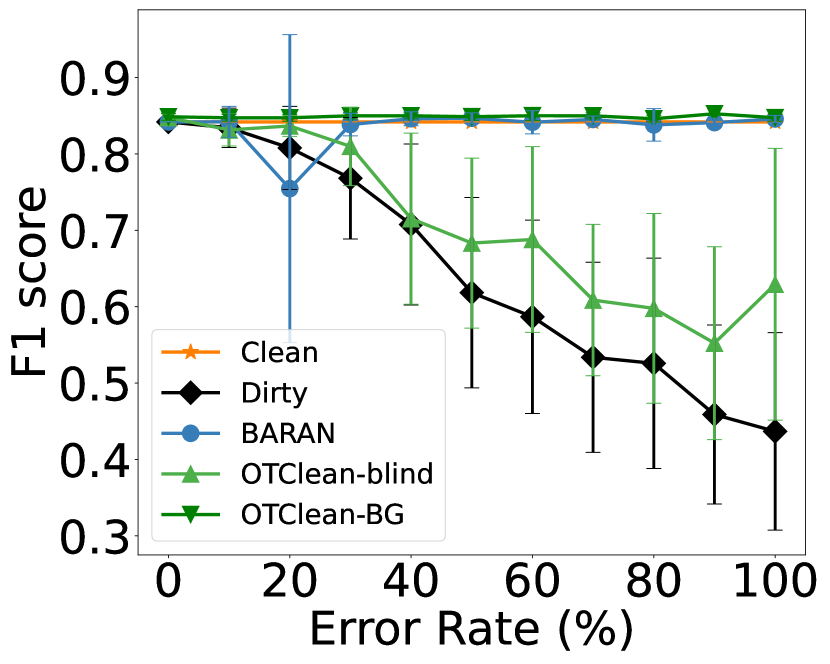
(d) Boston

Figure 6. Attribute noise

Attribute Noise

Figure 6 shows our results for cleaning data with attribute noise. We compared the performance, in terms of AUC and F1-score, of models using “Clean” data, “Dirty” data, and data cleaned by OTClean and Baran. Our cleaning algorithm only applies the CI constraint and does not need prior information about the noise type. However, it can also use knowledge about which attribute is noisy for repair. We tested OTClean in two ways: “blind”, without knowing the noisy attribute, and with background knowledge (BG), where the noisy attribute is identified. The figures show how accuracy changes with different levels of noise. As noise increases, the model trained on dirty data performs worse. In contrast, the model trained on OTClean-cleaned data in both scenarios closely matches the ground truth model’s behavior. This is because the dirty data model might learn false patterns not present in clean test data. However, using OTClean to apply the CI constraint helps the model focus on the correct data patterns. While OTClean improves accuracy in both the blind and BG-informed settings, using background knowledge generally leads to better performance than the blind approach and Baran.

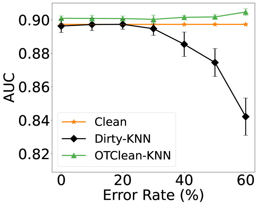
(a) kNN Imputation

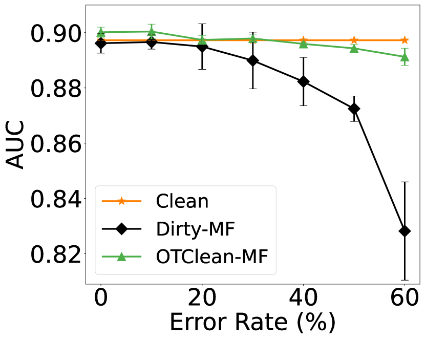
(b) Most Frequent

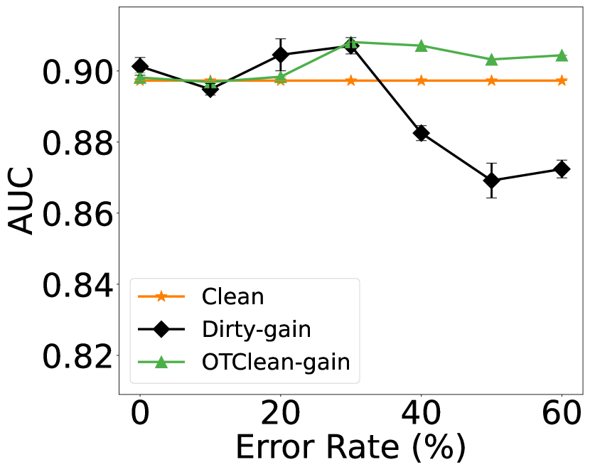
(c) GAIN

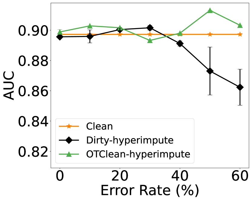
(d) Hyperimpute

Figure 7. Missing at random (MAR) in Boston dataset

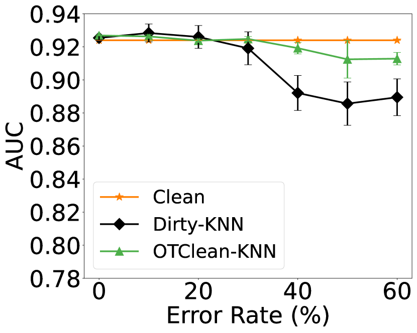
(a) kNN Imputation

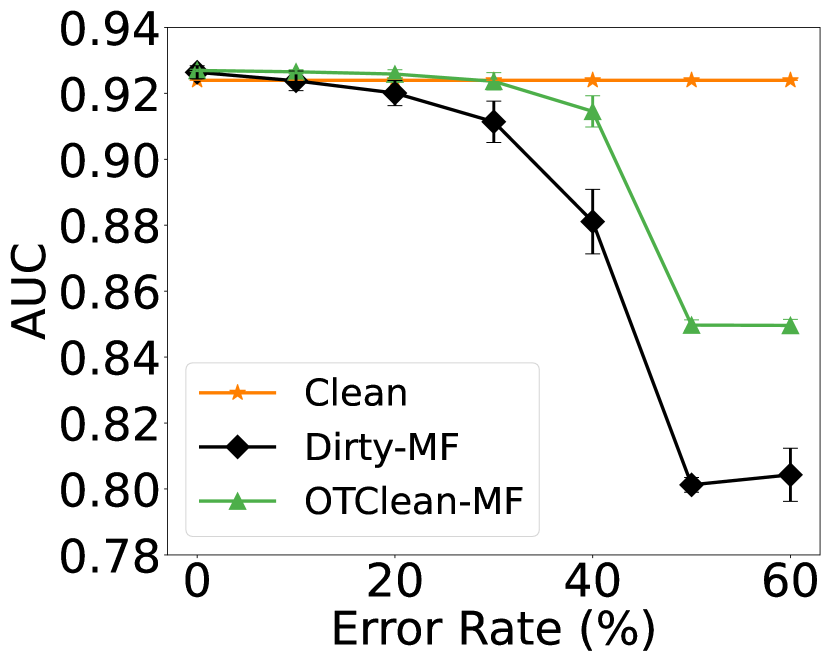
(b) Most Frequent

(c) GAIN

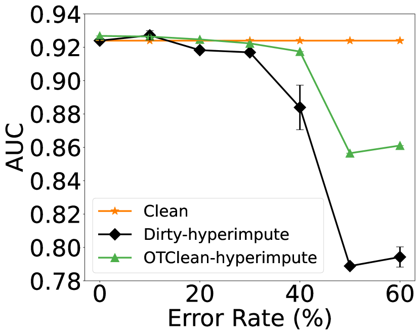
(d) Hyperimpute

Figure 8. Missing Not at Random (MNAR) in Car dataset

Missing Values

In our missing value experiments (Figures 7 for MAR and 8 for MNAR), we tested model performance at different missing data levels. We compared “Dirty” models (trained with missing values filled using methods like MF, kNN, GAIN, and Hyperimpute) against OTClean-enhanced models (OTClean-MF, OTClean-KNN, OTClean-GAIN, and OTClean-Hyperimpute). For MAR, all imputation methods struggled with high missing data rates, affecting performance. However, combining them with OTClean improved results, closely matching the ground truth regardless of missing data amount. The slight advantage over ground truth models in Figure 7 is due to limited data size. For MNAR, as shown in Figure 8, our approach performed better than the baseline but declined as missing data increased. This is because MNAR issues are generally harder to address. While using OTClean helps reduce false correlations, differences in training and test data distributions can still affect performance.

6.4. Evaluation using Statistical Distortion

Dasu et al. (Dasu and Loh, 2012) proposed a way to evaluate data cleaning methods, focusing on how they statistically distort data. They used measurements like the Earth Mover Distance (EMD) to see how much a method changes the original data distribution; less change is better. Their approach starts with a dirty dataset and its cleaned version. Using sampling, they generate pairs of these datasets, called replications, and clean the dirty ones. Using several replications instead of a single dataset pair ensures a more comprehensive and robust evaluation, avoiding biases that might arise from the unique characteristics of a single dataset. They then measure how much these strategies alter the data and improve error correction.

In our experiments, we applied this framework to test OTClean as a data cleaning method. We compared its effect on data distortion to other methods. Instead of looking at repaired errors, we focused on the accuracy (AUC) using the cleaned data. We ran 100 replications with attribute noise. The results are in Figure 9, where each cluster represents a cleaning method (the black point shows the original dirty data). Each point shows the balance between data distortion and AUC improvement for a replication. The figure indicates that OTClean generally improves performance more than Baran in most cases and is closer to the clean datasets, though with a bit more distortion. This increased distortion is due to moving the data closer to the ideal clean dataset, leading to better accuracy.

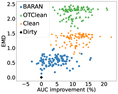
Figure 9. Comparing OTClean and the competing cleaning methods based on their statistical distortion

Dataset	FastOTClean-C1	FastOTClean-C2	MF	IC	MS	QCLP
Adult	1229	1279	66	66	700	NA
COMPAS	848	337	7	6	1227	2

Table 3. Runtime (sec) for the fairness application

6.5. OTClean’s Runtime and Performance

Runtime

In Table 3, we provide the runtime results of FastOTClean for Adult and COMPAS datasets, comparing them with the baselines. While our algorithm’s runtime is somewhat higher due to the complex nature of optimal transport, it remains reasonably fast and offers a practical means for employing optimal transport in data cleaning for CI constraints. Our algorithm’s runtime is mainly influenced by the number of attributes in the CI constraints rather than the data size. This is because the size of the transport plan we use stays the same no matter how large the data is; it only changes based on the number of attributes. In our experiments, the key factor is the domain size, determined by the number of attributes in the CI constraints and the range of values these attributes can take. Figure 10(a) illustrates FastOTClean’s runtime and memory usage for methods on the Adult for increasing domain size, showing that it can scale effectively to high-dimensional CIs. Furthermore, memory requirements and runtime can be further reduced by implementing a sparse representation for the transport plan.

Convergence and Optimization

Figure 10(b) demonstrates the convergence behavior of our main FastOTClean, affirming the result presented in Theorem 4.3. It shows the monotonic decrease of the objective function, which represents the cost of the transport plan with the number of iterations. Additionally, the graph compares the convergence properties of FastOTClean with two different initializations: one with a random initialization of q and another using NMF. Notably, initializing with NMF reduces the total convergence iterations by nearly 30%. We also highlight optimizations aimed at reducing runtime. The first optimization involves updating $q$ slices in parallel, achieving a significant speedup of  $\times 7$ in our Adult data. Another optimization focuses on unsaturated CIs. Figure 11(a) illustrates the substantial runtime improvement achieved by employing the proposed optimization for unsaturated CI constraints while maintaining the same outcome. In this scenario, we initiate with a CI constraint and construct ${\mathbf{W}}$ using attributes with varying domain sizes. We then evaluate the runtime of both the naive and saturation approaches. The saturation approach consistently solves the same problem, optimizing $\pi_{s}$, regardless of growing $\pi$’s size, contributing to its stable performance. In our final experiment, we investigate the impact of warm start optimization on Sinkhorn iteration numbers. Figure 11(b) shows warm start reduces the number of iterations by more than sevenfold.

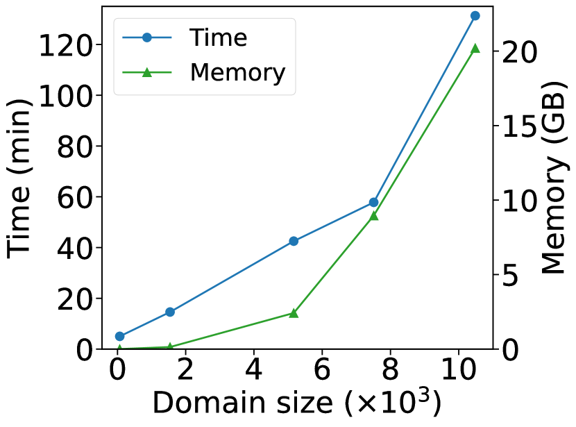
(a) Runtime and Memory Usage

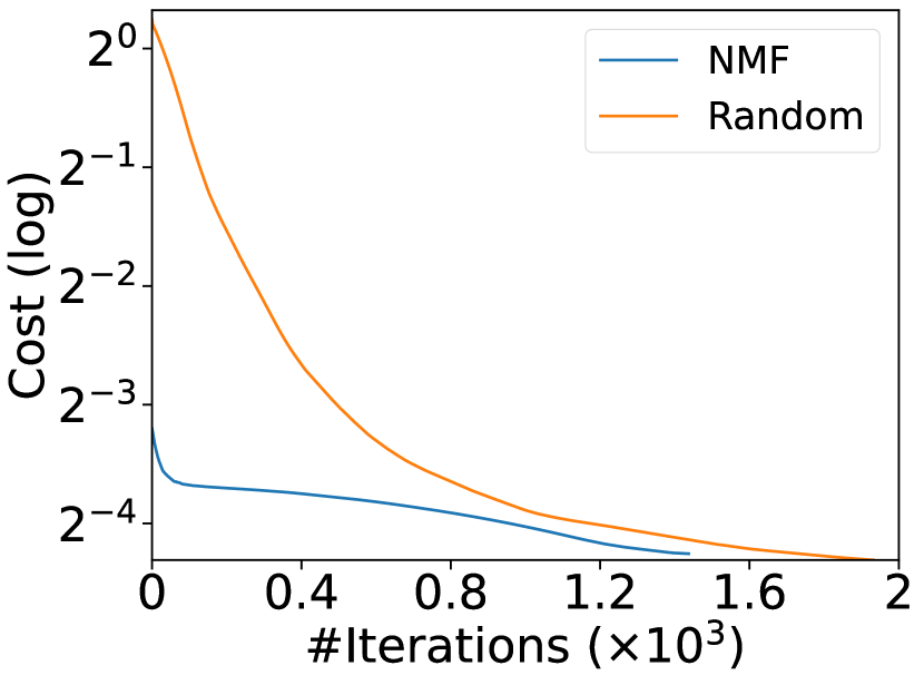
(b) Convergence

Figure 10. OTClean’ performance

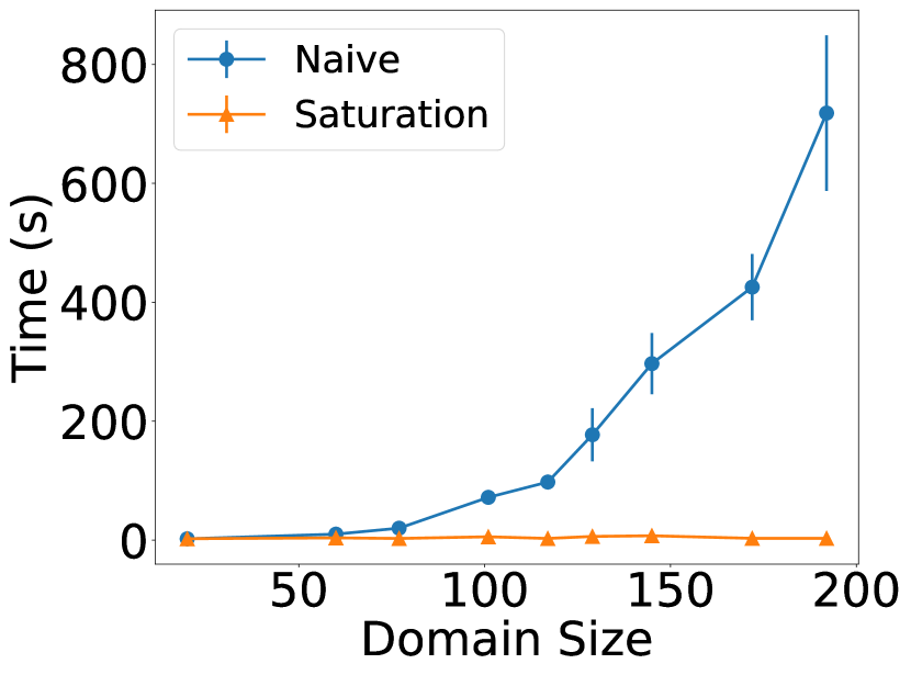
(a) Saturation

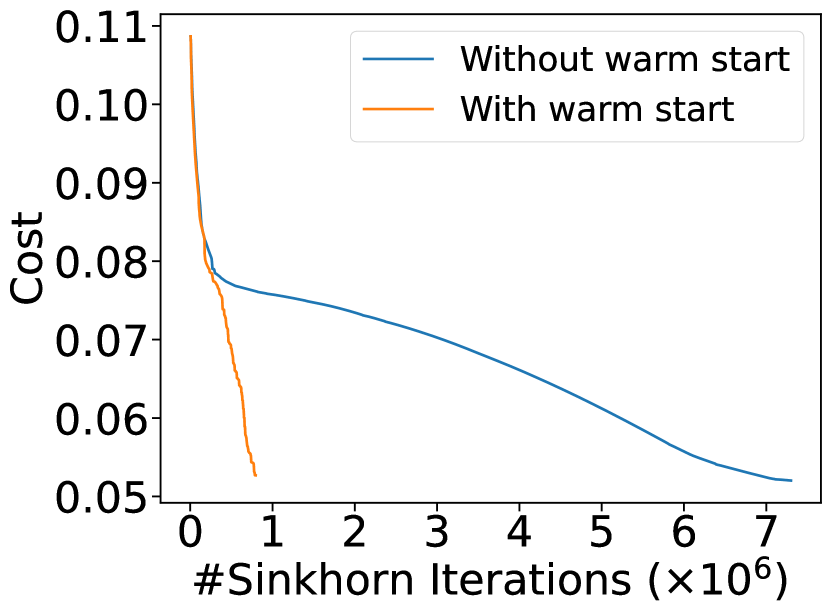
(b) Warm start

Figure 11. OTClean’s Optimizations

7. Related Work

Our research connects with two main areas of study.

Data Cleaning for Conditional Independence

Data cleaning in the database domain traditionally revolves around enforcing integrity constraints, such as functional dependencies and conditional functional dependencies (Livshits et al., 2020; Kolahi and Lakshmanan, 2009; Bohannon et al., 2006; Livshits and Kimelfeld, 2022). Nonetheless, the domain of data cleaning for conditional independence has only recently gained attention. Notable works in this emerging field include (Salimi et al., 2019) and (Yan et al., 2020). SCODED (Yan et al., 2020) employs statistical constraints to detect errors within datasets but primarily focuses on ranking individual data tuples based on their relevance to conditional independence violations, differing from our data-centric approach. On the other hand, (Salimi et al., 2019) aims to find optimal repairs for conditional independence violations, involving the addition or removal of tuples to satisfy the constraint. However, their method lacks the application of specific statistical divergence or distance measures to assess the quality of the repaired data. In a somewhat distinct vein, (Ahuja et al., 2021) utilizes generative adversarial networks (GANs) to generate data adhering to conditional independence constraints. Their primary objective is to train these generative models effectively, particularly emphasizing the minimization of Jensen–Shannon divergence in continuous data. However, their focus is on training generative models rather than cleaning existing data.

Fairness and Optimal Transport

Algorithmic fairness research has primarily focused on detecting and mitigating biases in machine learning models, utilizing pre-, post-, and in-processing techniques. Pre-processing methods (Caton and Haas, 2023), aim to eliminate bias from training data before model training. While model-agnostic approaches such as (Calmon et al., 2017; Feldman et al., 2015; Salimi et al., 2019) exist, they often lack insights into the root causes of biases. These strategies typically address basic fairness criteria and may not delve into enforcing conditional independence tests or incorporating optimal transport methods. Notably, (Gordaliza et al., 2019) employs the Wasserstein barycenter for pre-processing training data to achieve statistical parity but doesn’t specifically address the complexities of conditional statistical inference in high-dimensional datasets, distinguishing it from our approach. (Silvia et al., 2020) employs optimal transport as a regularizer during ML model training, focusing on a different aspect than our data cleaning objective. Additionally, studies like (Si et al., 2021; Black et al., 2020) use optimal transport to quantify unfairness, making them less aligned with our core research goal.

8. Conclusion

In this paper, we introduced a principled approach for data cleaning under conditional independence constraints, harnessing optimal transport theory. Our results underscore the importance of prioritizing conditional independence in data pipelines for enhancing ML model robustness, reliability, accuracy, and fairness. Our techniques have demonstrated potential with discrete data, and we aim to further optimize and extend their applicability to continuous and relational data. Additionally, we plan to explore methods for enforcing multiple conditional independence constraints and capturing interactions between CIs and other database dependencies.

9. Additional Experimental Results

In this section, we present additional experimental findings that couldn’t fit into the main paper due to space limitations.

9.1. Impact of Cost Functions

One of the key promises of OTClean is that by using OT, we can incorporate a suitable cost function that allows our solution to tailor its data repair based on the types of errors. To validate this concept, we conducted experiments to examine the impact of different cost functions on the results of our data-cleaning application.

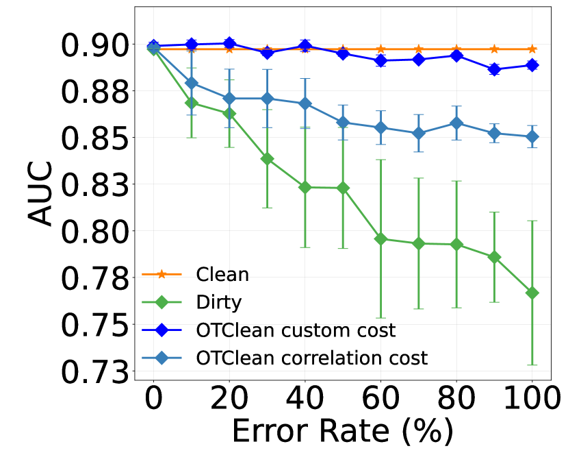
(a) Boston

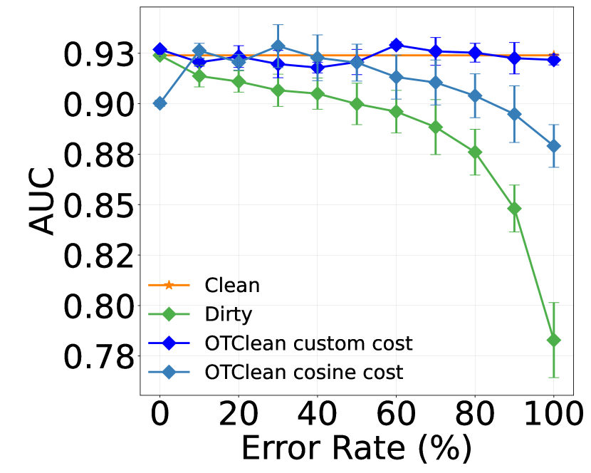
(b) Car

Figure 12. Impact of cost on cleaning

In particular, we focused on attribute noises, and we illustrate the outcomes in Figures 12. We carried out the experiments for attribute noise, as discussed in Section 6.3, but using various cost functions. The outcomes are presented in Figures 12(a) and 12(b), for datasets Boston and Car. In these experiments, we explored a user-defined or “custom” cost function that aligns with the noise introduction process. This custom cost function assigns lower repair costs to noisy values when they are more likely to be corrected to their true values. This indicates that fixing values with higher probabilities of being correct is easier and incurs lower costs compared to other potential corrections. We compare this custom cost function, denoted as “OTClean custom cost”, with two alternative cost functions. One is based on cosine similarity, denoted by “OTClean cosine cost”, in the Boston dataset, while the other uses Pearson correlation, denoted by “OTClean correlation cost”, in the Car dataset.

The results align with our expectations, demonstrating that a suitable custom cost function can come close to the clean data by effectively repairing noisy values to their true states. As shown in the figures, repairs made using the customer cost function result in a model that significantly outperforms the performance of the models using the other two general-purpose cost functions.

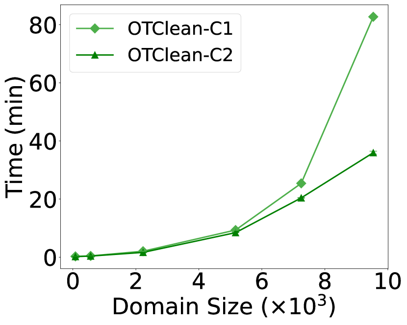
(a) Adult

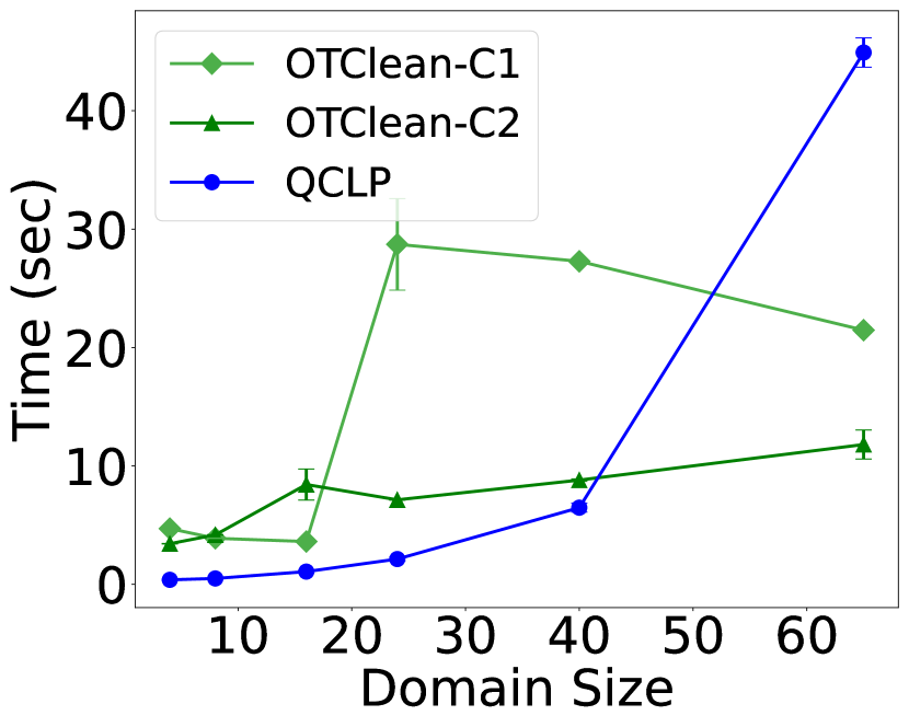
(b) COMPAS with QCLP

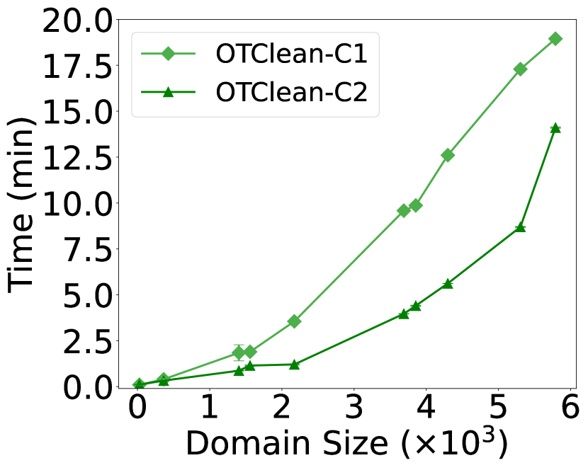
(c) COMPAS

Figure 13. Runtime

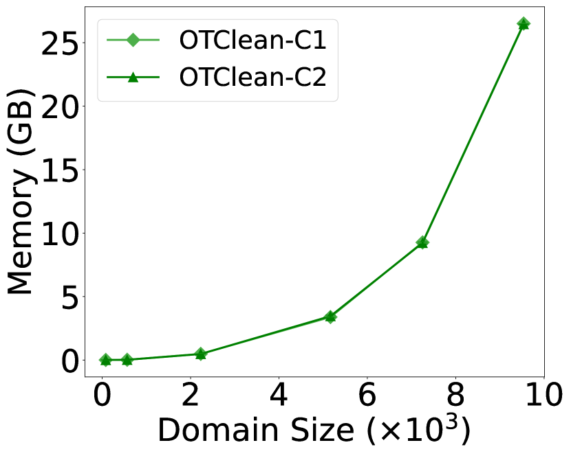
(a) Adult

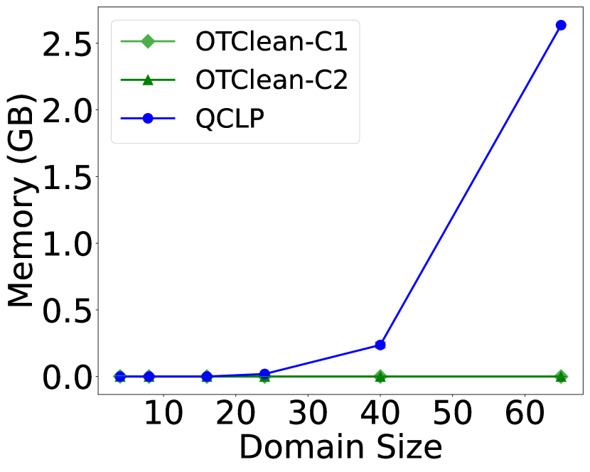
(b) COMPAS with QCLP

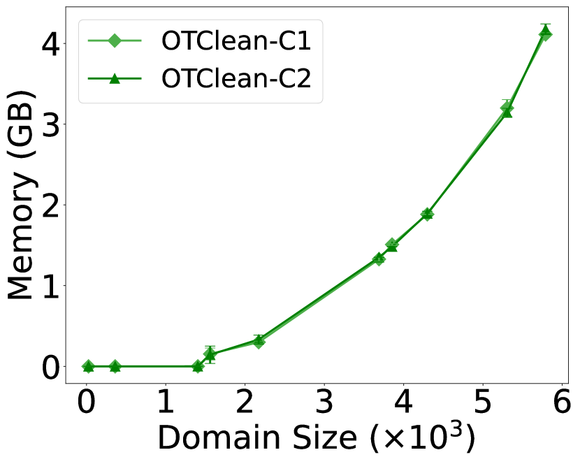
(c) COMPAS

Figure 14. Memory Usage

9.2. Runtime and Memory Analysis: FastOTClean vs QCLP

We conducted additional experiments to assess the performance of FastOTClean and compare it with QCLP. To assess the runtime performance and memory usage of FastOTClean and QCLP, we used the Adult and COMPAS datasets. The experiments are similar to those described in Section 6.5, which involves incrementally adding attributes to the CI constraints from these datasets to enlarge the domain size. This process allows us to analyze how increasing domain sizes affect both solutions’ runtime and memory usage. The outcomes of this analysis are illustrated in Figures 13 and 14.

In Figure 13(a), we present the runtime performance of FastOTClean on the Adult dataset across a range of domain sizes, using the two cost functions detailed in Section LABEL:sec:tunning. We omitted QCLP from this figure due to its prohibitively high memory demands, which resulted in failure at even the smallest domain sizes for Adult. The figure demonstrates that FastOTClean efficiently manages CI constraints involving multiple attributes, even in scenarios with extensive domain sizes.

Figure 13(b) contrasts the runtime performance of FastOTClean and QCLP in the COMPAS dataset, focusing on smaller domain sizes where QCLP does not fail. For larger domain sizes, Figure 13(c) specifically examines the runtime changes in FastOTClean, as QCLP fails in these conditions. These findings corroborate the data presented in Table 3, offering a broader perspective on how different domain sizes impact performance. Notably, the runtimes recorded in Table 3 for small domain sizes in COMPAS indicate QCLP’s superior performance in these specific conditions, although FastOTClean exhibits better performance across other domain sizes, as shown in Figure 13(b).

Finally, Figure 14 presents the memory usage of both FastOTClean and QCLP. Like the runtime analysis, the memory consumption was examined for both Adult and COMPAS datasets. In the case of QCLP, memory usage data is available only for smaller domain sizes in COMPAS. The key insight from these observations is that FastOTClean consistently requires less memory than QCLP, especially as the domain size increases.

9.3. Integrating Background Knowledge

Another set of experiments focused on understanding how considering prior background knowledge about erroneous attributes affects our data repair process, especially when dealing with attribute noise. Figure 15 illustrates the difference in performance between models trained without knowledge of erroneous attributes (OTClean-Blind) and those trained with background knowledge (OTClean-BG). The results reveal that knowing which attributes to repair significantly improves our solution, almost matching the performance of a clean dataset. We provide results for the Boston dataset since the Car dataset already exhibited high performance with blind repair, leaving little room for improvement.

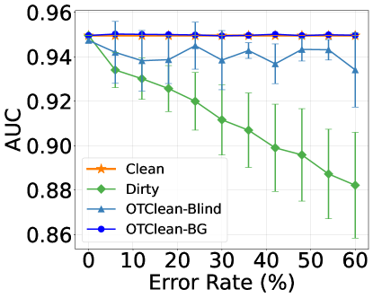
Figure 15. Blind Repair vs Repair with Background Knowledge

9.4. Additional Results for Missing Value

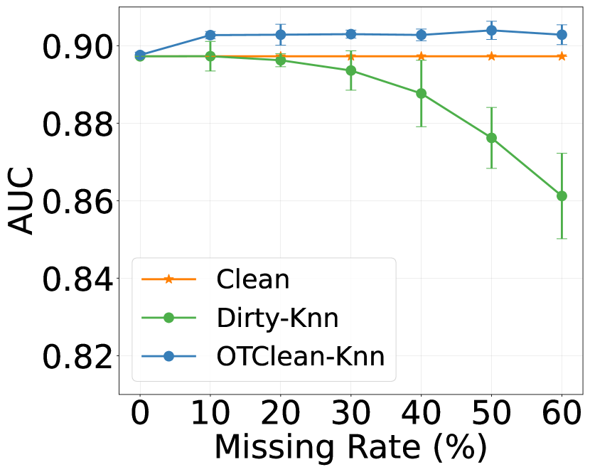
(a) kNN Imputation (Boston)

(b) Most Frequent (Boston)

Figure 16. Missing Not at Random (MNAR).

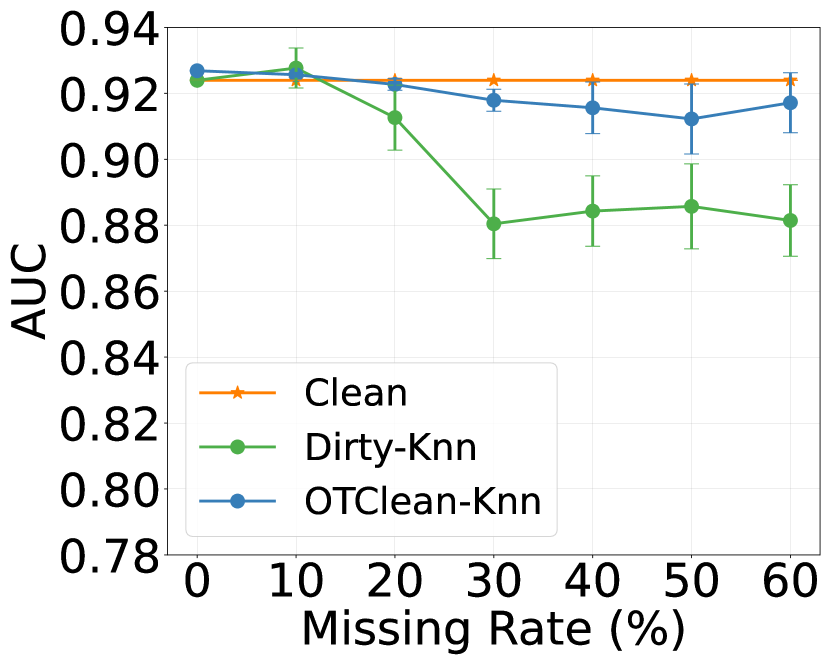
(a) kNN Imputation (Car)

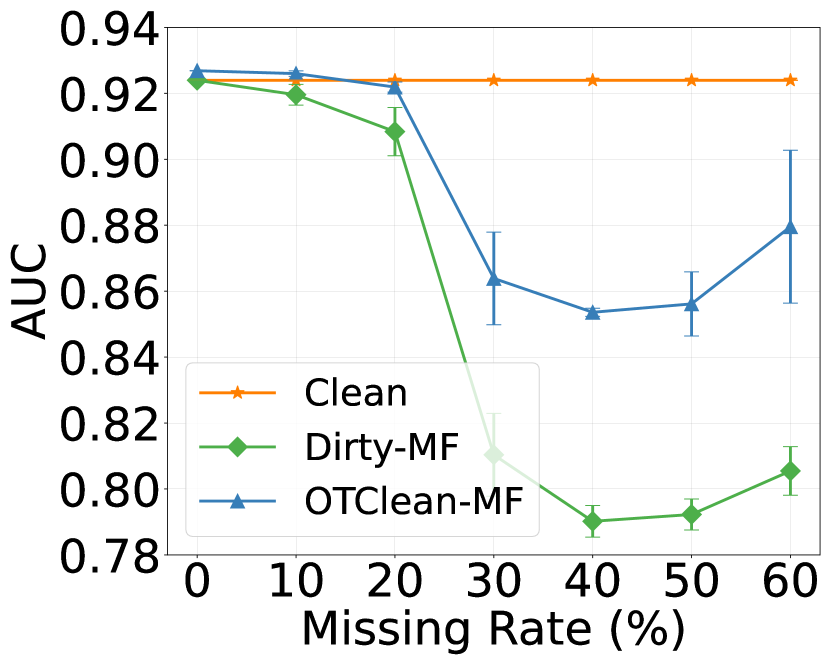
(b) Most Frequent (Car)

Figure 17. Missing at random (MAR)

We conducted extensive experiments on missing value imputation for both the Boston and Car datasets, including scenarios of MAR and MNAR. These additional experiments were not included in the main body of the paper but are presented in this section, as shown in Figures 16 and 17.

The results reaffirm our earlier conclusions regarding the effectiveness of OTClean in repairing data to mitigate the spurious correlations introduced by imputation methods employed to handle missing values. This is particularly more evident in Figures 16(a)-17(a). As illustrated in Figure 17(b), the efficacy of OTClean is still contingent on both the initial imputation technique used and the missing data rate. Higher rates of missing values and the use of a simplistic imputation method like naive most-frequent (MF) imputation can lead to reduced performance, even after applying OTClean. Nevertheless, it is worth noting that OTClean consistently delivers significant improvements compared to imputation methods without subsequent repair.

References

- (1)
- adu (2023) 2023. Adult Data Set. https://archive.ics.uci.edu/ml/datasets/adult
- bos (2023) 2023. The Boston Housing Dataset. https://www.cs.toronto.edu/~delve/data/boston/bostonDetail.html
- car (2023) 2023. Car Evaluation Data Set. https://archive.ics.uci.edu/ml/datasets/Car+Evaluation UCI Machine Learning Repository.
- com (2023) 2023. COMPAS Analysis. https://github.com/propublica/compas-analysis/
- Ahuja et al. (2021) Kartik Ahuja, Prasanna Sattigeri, Karthikeyan Shanmugam, Dennis Wei, Karthikeyan Natesan Ramamurthy, and Murat Kocaoglu. 2021. Conditionally Independent Data Generation. In UAI. 2050–2060.
- Arjovsky et al. (2019) Martin Arjovsky, Léon Bottou, Ishaan Gulrajani, and David Lopez-Paz. 2019. Invariant Risk Minimization. arXiv preprint arXiv:1907.02893 (2019).
- Arjovsky et al. (2017) Martin Arjovsky, Soumith Chintala, and Léon Bottou. 2017. Wasserstein Generative Adversarial Networks. In ICML. 214–223.
- Bertossi (2006) Leopoldo Bertossi. 2006. Consistent Query Answering in Databases. ACM SIGMOD Record 35, 2 (2006), 68–76.
- Black et al. (2020) Emily Black, Samuel Yeom, and Matt Fredrikson. 2020. FlipTest: Fairness Testing via Optimal Transport. In FAccT. 111–121.
- Bohannon et al. (2006) Philip Bohannon, Wenfei Fan, Floris Geerts, Xibei Jia, and Anastasios Kementsietsidis. 2006. Conditional Functional Dependencies for Data Cleaning. In ICDE. 746–755.
- Boyd et al. (2004) Stephen Boyd, Stephen P Boyd, and Lieven Vandenberghe. 2004. Convex Optimization. Cambridge University Press.
- Boyd et al. (2011) Stephen Boyd, Neal Parikh, Eric Chu, Borja Peleato, Jonathan Eckstein, et al. 2011. Distributed Optimization and Statistical Learning via the Alternating Direction Method of Multipliers. Foundations and Trends® in Machine Learning 3, 1 (2011), 1–122.
- Bozdag (2013) Engin Bozdag. 2013. Bias in Algorithmic Filtering and Personalization. Ethics and Information Technology 15, 3 (2013), 209–227.
- Calmon et al. (2017) Flavio Calmon, Dennis Wei, Bhanukiran Vinzamuri, Karthikeyan Natesan Ramamurthy, and Kush R Varshney. 2017. Optimized Pre-Processing for Discrimination Prevention. NeurIPS 30 (2017).
- Caton and Haas (2023) Simon Caton and Christian Haas. 2023. Fairness in Machine Learning: A Survey. Computing Surveys (2023).
- Cover (1999) Thomas M Cover. 1999. Elements of Information Theory. John Wiley & Sons.
- Cuturi (2013) Marco Cuturi. 2013. Sinkhorn Distances: Lightspeed Computation of Optimal Transport. NeurIPS 26 (2013).
- Dasu and Loh (2012) Tamraparni Dasu and Ji Meng Loh. 2012. Statistical Distortion: Consequences of Data Cleaning. VLDB 5, 11 (2012).
- Fan and Geerts (2022) Wenfei Fan and Floris Geerts. 2022. Foundations of Data Quality Management. Springer Nature.
- Feldman et al. (2015) Michael Feldman, Sorelle A. Friedler, John Moeller, Carlos Scheidegger, and Suresh Venkatasubramanian. 2015. Certifying and Removing Disparate Impact. In KDD. 259–268.
- Finesso and Spreij (2004) Lorenzo Finesso and Peter Spreij. 2004. Approximate Nonnegative Matrix Factorization via Alternating Minimization. arXiv preprint math/0402229 (2004).
- Frogner et al. (2015) Charlie Frogner, Chiyuan Zhang, Hossein Mobahi, Mauricio Araya, and Tomaso A Poggio. 2015. Learning with a Wasserstein Loss. NeurIPS 28 (2015).
- Galhotra et al. (2021) Sainyam Galhotra, Romila Pradhan, and Babak Salimi. 2021. Explaining Black-Box Algorithms using Probabilistic Contrastive Counterfactuals. In SIGMOD. 577–590.
- Gordaliza et al. (2019) Paula Gordaliza, Eustasio Del Barrio, Gamboa Fabrice, and Jean-Michel Loubes. 2019. Obtaining Fairness using Optimal Transport Theory. In ICML. 2357–2365.
- Guyon and Elisseeff (2003) Isabelle Guyon and André Elisseeff. 2003. An Introduction to Variable and Feature Selection. JMLR 3, Mar (2003), 1157–1182.
- Hajian et al. (2016) Sara Hajian, Francesco Bonchi, and Carlos Castillo. 2016. Algorithmic Bias: From Discrimination Discovery to Fairness-Aware Data Mining. In KDD. 2125–2126.
- Hien and Gillis (2021) Le Thi Khanh Hien and Nicolas Gillis. 2021. Algorithms for Nonnegative Matrix Factorization with the Kullback–Leibler Divergence. SISC 87, 3 (2021), 1–32.
- Hooker (2021) Sara Hooker. 2021. Moving Beyond “Algorithmic Bias is a Data Problem”. Patterns 2, 4 (2021), 100241.
- Jarrett et al. (2022) Daniel Jarrett, Bogdan C Cebere, Tennison Liu, Alicia Curth, and Mihaela van der Schaar. 2022. Hyperimpute: Generalized Iterative Imputation with Automatic Model Selection. In ICML. 9916–9937.
- Kolahi and Lakshmanan (2009) Solmaz Kolahi and Laks VS Lakshmanan. 2009. On Approximating Optimum Repairs for Functional Dependency Violations. In ICDT. 53–62.
- Koller and Friedman (2009) Daphne Koller and Nir Friedman. 2009. Probabilistic Graphical Models: Principles and Techniques. MIT press.
- Koller et al. (1996) Daphne Koller, Mehran Sahami, et al. 1996. Toward Optimal Feature Selection. In ICML, Vol. 96. 292.
- Lee and Seung (2000) Daniel Lee and H Sebastian Seung. 2000. Algorithms for Non-Negative Matrix Factorization. NeurIPS 13 (2000).
- Livshits and Kimelfeld (2022) Ester Livshits and Benny Kimelfeld. 2022. The Shapley Value of Inconsistency Measures for Functional Dependencies. LMCS 18 (2022).
- Livshits et al. (2020) Ester Livshits, Benny Kimelfeld, and Sudeepa Roy. 2020. Computing Optimal Repairs for Functional Dependencies. TODS 45, 1 (2020), 1–46.
- Magliacane et al. (2018) Sara Magliacane, Thijs Van Ommen, Tom Claassen, Stephan Bongers, Philip Versteeg, and Joris M Mooij. 2018. Domain Adaptation by Using Causal Inference to Predict Invariant Conditional Distributions. NeurIPS 31 (2018).
- Mahdavi and Abedjan (2020) Mohammad Mahdavi and Ziawasch Abedjan. 2020. Baran: Effective Error Correction via a Unified Context Representation and Transfer Learning. VLDB 13, 12 (2020), 1948–1961.
- Pearl et al. (2009) Judea Pearl et al. 2009. Causal Inference in Statistics: An Overview. Statistics Surveys 3 (2009), 96–146.
- Pele and Werman (2009) Ofir Pele and Michael Werman. 2009. Fast and Robust Earth Mover’s Distances. In ICCV. 460–467.
- Pogodin et al. (2023) Roman Pogodin, Namrata Deka, Yazhe Li, Danica J Sutherland, Victor Veitch, and Arthur Gretton. 2023. Efficient Conditionally Invariant Representation Learning. ICLR (2023).
- Rojas-Carulla et al. (2018) Mateo Rojas-Carulla, Bernhard Schölkopf, Richard Turner, and Jonas Peters. 2018. Invariant Models for Causal Transfer Learning. JMLR 19, 1 (2018), 1309–1342.
- Salimi et al. (2019) Babak Salimi, Luke Rodriguez, Bill Howe, and Dan Suciu. 2019. Interventional Fairness: Causal Database Repair for Algorithmic Fairness. In SIGMOD. 793–810.
- Si et al. (2021) Nian Si, Karthyek Murthy, Jose Blanchet, and Viet Anh Nguyen. 2021. Testing Group Fairness via Optimal Transport Projections. In ICML. 9649–9659.
- Silvia et al. (2020) Chiappa Silvia, Jiang Ray, Stepleton Tom, Pacchiano Aldo, Jiang Heinrich, and Aslanides John. 2020. A General Approach to Fairness with Optimal Transport. In AAAI, Vol. 34. 3633–3640.
- Sinkhorn (1964) Richard Sinkhorn. 1964. A relationship Between Arbitrary Positive Matrices and Doubly Stochastic Matrices. The Annals of Mathematical Statistics 35, 2 (1964), 876–879.
- Torralba and Efros (2011) Antonio Torralba and Alexei A Efros. 2011. Unbiased Look at Dataset Bias. In CVPR. 1521–1528.
- Tseng (2001) Paul Tseng. 2001. Convergence of a Block Coordinate Descent Method for Nondifferentiable Minimization. JOTA 109, 3 (2001), 475.
- Van de Panne (1966) C Van de Panne. 1966. Programming with a Quadratic Constraint. Management Science 12, 11 (1966), 798–815.
- Weinberger and Tesauro (2007) Kilian Q Weinberger and Gerald Tesauro. 2007. Metric Learning for Kernel Regression. In AISTATS. 612–619.
- Wong et al. (2000) SK Michael Wong, Cory J Butz, and Dan Wu. 2000. On the Implication Problem for Probabilistic Conditional Independency. SMC 30, 6 (2000), 785–805.
- Yan et al. (2020) Jing Nathan Yan, Oliver Schulte, MoHan Zhang, Jiannan Wang, and Reynold Cheng. 2020. SCODED: Statistical Constraint Oriented Data Error Detection. In SIGMOD. 845–860.
- Yoon et al. (2018) Jinsung Yoon, James Jordon, and Mihaela Schaar. 2018. GAIN: Missing Data Imputation using Generative Adversarial Nets. In ICML. 5689–5698.