Towards Optimal Customized Architecture for Heterogeneous Federated Learning with Contrastive Cloud-Edge Model Decoupling

Abstract

Federated learning, as a promising distributed learning paradigm, enables collaborative training of a global model across multiple network edge clients without the need for central data collecting. However, the heterogeneity of edge data distribution drags the model towards the local minima, which can be distant from the global optimum. Such heterogeneity often leads to slow convergence and substantial communication overhead. To address these issues, we propose a novel federated learning framework called FedCMD, a model decoupling tailored to the Cloud-edge supported federated learning that separates deep neural networks into a body for capturing shared representations in Cloud and a personalized head for migrating data heterogeneity. Our motivation is that, by the deep investigation of the performance of selecting different neural network layers as the personalized head, we found rigidly assigning the last layer as the personalized head in current studies is not always optimal. Instead, it is necessary to dynamically select the personalized layer that maximizes the training performance by taking the representation difference between neighbor layers into account. To find the optimal personalized layer, we utilize the low-dimensional representation of each layer to contrast feature distribution transfer and introduce a Wasserstein-based layer selection method, aimed at identifying the best-match layer for personalization. Additionally, a weighted global aggregation algorithm is proposed based on the selected personalized layer for the practical application of FedCMD. Extensive experiments on ten benchmarks demonstrate the efficiency and superior performance of our solution compared with nine state-of-the-art solutions. All code and results are available at https://github.com/elegy112138/FedCMD.

I Introduction

Impressive capacity magnification in wireless communication technologies has catalyzed a significant expansion in the capabilities of mobile devices, wearables, and other internet-connected devices. These devices boast advanced hardware and software, enabling the support of various applications and the generation of extensive volumes of contextual and user-specific data. Due to privacy concerns and the enhanced computing and storage capacities at the network edge, there is an increasing preference to store data locally on edge devices [1, 2]. This shift facilitates the execution of the model training on these devices using locally available data, with only sporadic communication with a central parameter server. This decentralized methodology, known as federated learning [3], is a stark departure from traditional model training, which typically relies on the central aggregation of raw data.

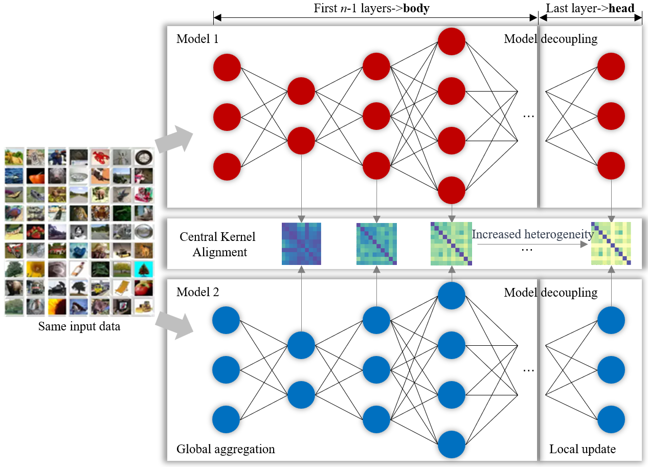
Figure 1: Model decoupling based on Central Kernel Alignment.

One of the most significant challenges in federated learning, as highlighted by recent research, is the heterogeneity of data distribution (non-independent and identically distributed, non-IID) across a multitude of client devices. In this scenario, where potentially thousands of devices participate, the heterogeneity can significantly impact the convergence of the model training and cause increased communication costs. This challenge is especially acute when training large-scale neural network models, such as transformer-based models, which are surprisingly difficult to train [4].

Addressing the adverse effects of data heterogeneity is a critical area of research, with numerous recent studies dedicated to developing solutions. These include approaches like knowledge distillation [6, 5, 7], loss regularization [8, 9, 10], similarity aggregation [12, 11, 13], and model decoupling [14, 15, 16]. Among these, model decoupling, a strategy that has gained prominence recently, stands out for its notable capability to significantly reduce communication overhead and enhance performance by strategically segmenting deep neural networks into a shared pre-output body and a distinct personalized head [15, 14]. As shown in Fig. 1, assuming the local model is an n-layer neural network, prior work [18, 14, 15, 17, 16] conventionally designated the first (n-1) layers as the body and the last layer as the personalized head. In this paradigm, the pre-output body parameters undergo global aggregation, while the personalized layer is only updated locally. This approach primarily aims to mitigate the adverse effects of heterogeneous data on shared partial parameters to the central server, thus enhancing the personalized performance [16].

However, this last-layer-as-head decoupling, rooted in Central Kernel Alignment (CKA) [14, 15, 16], does not demonstrate optimal guarantees in theory. CKA is used as the metric to evaluate the similarity of outputs of the same layer from two identical-structure models with the same input data. In scenarios where network edges with heterogeneous data distributions, the locally trained models process information layer-by-layer with the degree of heterogeneity of each layer’s outputs increasing throughout this progression. Based on this, current methods contend that the output of the final layer, exhibiting the highest heterogeneity, is most suitable for the personalized layer. This perspective fails to consider that the heterogeneity noted in the output of the last layer is not isolated, but rather the cumulative effect of all previous layers.

Moving from theoretical considerations to practical implications, we conducted extended experiments across ten real-world datasets with three different neural architectures also revealing that the last layer might not always be the best selection. These observations motivate us to rethink the existing last-layer-as-head design. Thus, we conducted an in-depth exploration for model decoupling and found three statistical discoveries based on the experiment results: (1) Selecting the last layer as the personalized layer is not the best option in most cases; (2) While multiple layers can be chosen as personalized head, optimal performance emerges from selecting the most appropriate single layer; (3) Consistency in choosing the same personalized layer across different clients is essential for fast and stable convergence of the model training. Building on the experimental findings, we also discovered that the criteria for selecting the personalized layer should consider both the input and output of each layer, rather than focusing only on the output as is typical in CKA-based solutions.

In this context, there is a need to find a new method that can knowledgeize the heterogeneity of data distribution across different users to facilitate the personalized layer selection. Thus, we first propose a layer-wise knowledgeization method to capture the low-dimensional feature distribution of the intermediate layers. Furthermore, a novel contrastive personalized layer selection mechanism based on Wasserstein distance [19] is proposed to identify the best-match layer. This method involves a layer-by-layer comparison to identify transfer in low-dimensional representational distributions of each layer. Subsequently, selecting the layer where the feature distribution transfer is minimized as the personalized layer. Extensive experimental testing has shown that choosing the layer with the minimal Wasserstein distance relative to the local data distribution as the personalized layer yields the best performance. Further, we developed a novel contrastive Cloud-edge model decoupling framework named FedCMD by dividing the Cloud-Edge federated learning into two main phases: the personalized layer selection phase and the heterogeneous federated learning phase. We also provided two piratical algorithms by selecting the personalized layer with the contrastive layer selection to migrate data heterogeneity at the edges and share the other layers’ parameters to the Cloud for collaborative learning. To the best of our knowledge, FedCMD represents the first attempt to introduce an alternative to the CKA standard for personalized layer selection, proposing the use of a non-final layer as the personalized layer in model decoupling. The main contributions of this work are as follows:

• Introducing a new distribution distance metric called feature distribution transfer for personalized layer selection, based on three findings discovered through extensive experimentation results on real-world datasets.

• Proposing a novel heterogeneous federated learning framework, termed FedCMD with two main phases based on the feature distribution shift distance. To the best of our knowledge, our work is the first exploration in facilitating personalized layer selection by quantifying the heterogeneity in their data distributions.

• Providing two practical algorithms for achieving personalized layer selection and weighted global aggregation across the Cloud-Edge federated learning system.

• Conducting comprehensive experiments, validating our solution’s performance superiority on ten datasets compared to nine other SOTA solutions.

The related works are reviewed in section II. Section III presents the motivation. Section IV provides the system model and preliminaries. Section V gives the details of the contrastive layer selection mechanism and FedCMD framework. Section VI introduces the algorithm design and implementation. In section VII, we evaluate our solution in five main parts with nine state-of-the-art solutions. Finally, section VIII concludes the paper and outlines directions for future work.

II Related Works

II-A Heterogeneous Federated Learning

Federated Learning such as FedAvg [3] is a method designed for privacy-preserving data sharing while allowing the training of models across distributed devices. However, traditional federated learning, mainly developed for scenarios with independent and identically distributed (iid) data distribution, struggles with slow convergence rates when applied to heterogeneous data distribution.

To address the challenge, heterogeneous federated learning has been proposed which encompasses several key aspects: (1) Knowledge distillation [5, 6, 7] refines the exchange of information between global and local models, enhancing model generalization capabilities. (2) Regularization terms in the loss function [8, 9, 10] are employed to correct biases towards the global model, improving the robustness and universality of the global model. (3) Similarity aggregation, such as clustering [11, 12, 13] and multi-task learning [11, 10, 20], enable more efficient information sharing among similar clients or tasks. Clustering groups like clients to learn individual models, whereas multi-task learning handles several client models simultaneously without forming distinct clusters. However, these methods often come with inherent drawbacks, such as relying on additional public datasets [5, 6, 7], increased computational complexity [8, 9, 10], and the risk of data leakage caused by additional parameter exposure [11, 10, 20, 12, 13]. One of the currently prominent approaches is (4) Model decoupling, which segregates models into shared body and personalized head. The body’s layers are shared among all clients, whereas the head is tailored based on each client’s data, striking a balance between global performance and individual client requirements.

TABLE I: Personalized layer performances of models with one fc and classifier across 10 datasets.

Configuration	CIFAR100	CIFAR10	CINIC10	EMNIST	FMNIST	M.N.A	M.N.C	MNIST	SVHN	T. ImageNet
fc1	40.346	85.265	80.27	92.968	96.548	94.192	92.897	98.827	92.990	22.345
classifier	43.647	84.556	78.792	93.635	96.750	96.017	94.376	99.336	93.873	28.201

TABLE II: Personalized layer performances of models with two fc and classifier across 10 datasets.

Configuration	CIFAR100	CIFAR10	CINIC10	EMNIST	FMNIST	M.N.A	M.N.C	MNIST	SVHN	T. ImageNet
fc1	42.698	86.263	80.500	93.188	96.420	95.096	85.742	98.956	93.302	21.740
fc2	47.541	86.940	80.575	93.994	96.599	96.487	94.172	99.421	94.654	31.056
classifier	42.925	84.282	78.983	93.554	96.403	95.588	94.029	99.363	94.240	28.061

TABLE III: Personalized layer performances of models with three fc and classifier across 10 datasets.

Configuration	CIFAR100	CIFAR10	CINIC10	EMNIST	FMNIST	M.N.A	M.N.C	MNIST	SVHN	T. ImageNet
fc1	39.340	86.110	80.230	93.096	96.633	94.807	92.603	98.874	93.732	20.487
fc2	46.895	87.088	80.677	93.825	96.701	96.645	94.623	99.381	95.042	30.135
fc3	44.975	84.305	79.060	94.000	96.366	95.985	94.147	99.337	94.669	30.732
classifier	39.723	83.512	78.282	87.407	90.933	95.514	92.837	98.261	89.523	27.444

TABLE IV: Performances comparison of multiple layers and single layer as the personalized layer across 10 datasets.

Configuration	CIFAR100	CIFAR10	CINIC10	EMNIST	FMNIST	M.N.A	M.N.C	MNIST	SVHN	T.ImageNet
fc2	47.541	86.940	80.575	93.994	96.599	96.487	94.172	99.421	94.654	31.056
fc1 & fc2	40.669	84.491	80.186	93.027	96.286	94.080	92.693	98.671	92.818	21.786
fc1 & classifier	40.735	85.265	80.260	93.001	96.407	94.721	93.068	98.859	93.144	21.716
fc2 & classifier	43.313	84.811	79.741	93.850	96.450	95.550	93.499	99.263	94.132	28.887
fc1 & fc2 & classifier	38.458	83.475	78.582	92.828	96.164	93.393	91.893	98.477	92.453	21.635

II-B Model Decoupling

Model decoupling is a critical approach that distinctly separates the fundamental and personalized layers of the model. Several pivotal methodologies, including FedRep [14], FedPer [21], and FedPav [22] achieve this by splitting client models into fundamental and personalized layers. In these models, the foundational layers are sent to the server for global aggregation, while the personalized layers are updated locally at each client. For instance, FedBN [23] and FedAP [24] use the batch normalization layer as the personalized component, keeping it local, with other layers participating in global aggregation to reduce feature drift. Notably, FedAP employs Wasserstein distance to assess the batch normalization layer’s data, aiding in setting aggregation weights. In contrast, FedBabu [15] and pFedSim [16] classify the final layer (classifier) as the head and earlier layers as the body. FedBabu uses a fixed head initialized randomly, while pFedSim updates the head locally and uses weighted global aggregation based on classifier distance. However, these methods are too rigid and inflexible in personalized layer selection, and cannot adapt the layer selection based on the specific situation. Compared to existing methods, our work presents several notable distinctions and advantages. Firstly, we conducted an extensive exploration of the current last-layer-as-head decoupling design and gave three findings in Section III. Secondly, we proposed a novel contrastive layer selection mechanism based on Wasserstein distance. Lastly, leveraging the personalized layer selection outcomes, we further devised a weighted global aggregation approach to enhance personalized performance.

III Motivation

We present motivation from three perspectives: (1) identifying the best layer for personalization, (2) evaluating whether multiple layers could enhance performance, and (3) determining if the optimal personalized layers vary across different clients with heterogeneous data distributions.

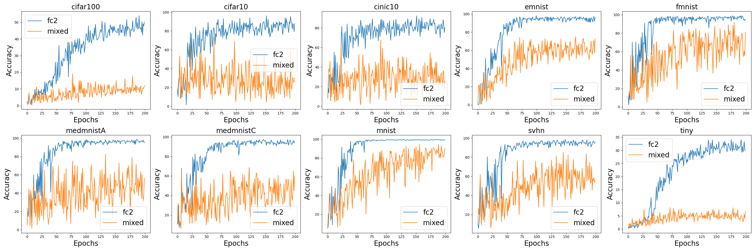
Figure 2: Performance comparison of the mixed personalized layer approach and the fc2 personalized layer method across ten datasets.

III-A Performance comparison with different personalized layer

Studies like FedRep [14], FedBadu [15] and pFedSim [16], which adopt Central Kernel Alignment theory, typically define the first (n-1) layers of a neural network as the body and the last layer as personalized head. However, our experiments with three different neural architectures across ten datasets (more details, please refer to Appendix -A) and as illustrated in Tables I–III, we observed that the pre-output fully connected (fc) layer performs better than the last layer (classifier) as the personalized layer in most cases. We tested three versions of the LeNet5 [25] model, each with a different number of fc layers (2, 3, and 4 layers), across ten standard datasets. In the 2-layer model as shown in Table I, the classifier layer showed better results than the first fc layer (fc1) when used as the personalized layer. For the 3-layer LeNet5 as shown in Table II, the second fc layer (fc2) yielded the highest performance when used as the personalized layer across all datasets. With the 4-layer model as shown in Table III, both the fc2 and third fc layers (fc3) demonstrated superior performance compared to using the classifier as the personalized layer. The results indicate that the classifier is not always the best choice. This finding across these configurations highlights the need to develop a new mechanism for personalized layer selection.

III-B Multi-layer personalization evaluation

Recent studies such as FedTSDP [26] and PCCFED [27], are exploring the use of multiple fc layers as the personalized layer. To investigate whether employing a combination of fc layers as the personalized layer could enhance performance, we conducted experiments with the 3-layer LeNet5 model. As shown in Table. IV, we compared the performance of using just the fc2 layer as the personalized layer against four combinations: (1) fc1+fc2, (2) fc1+classifier, (3) fc2+classifier, and (4) fc1+fc2+classifier. Our findings reveal that the performance of the single fc2 layer always surpassed the combinations. This suggests that selecting multiple layers as the personalization does not lead to performance improvement.

III-C Heterogeneity of clients in personalized layer selection

Our experiment results also revealed that despite all clients selecting fc2 as their personalized layer, the performance of their local models varied. This observation prompted us to explore the possibility that clients with heterogeneous data distributions may benefit from having different personalized layers. We conducted experiments where clients that showed poor performance with fc2 as their personalized layer were reassigned to use the classifier instead. This adjustment was implemented to evaluate the effectiveness of a mixed personalized layer case on the model training. However, this mixed solution did not enhance model performance and led to slow convergence in ten different datasets, as shown in Fig. 2. Based on the above results, our solution will focus on the design where all clients choose one common personalized layer.

TABLE V: Mathematical Notations

Symbol	Description
$\mathcal{G}(\mathcal{V},\mathcal{L})$	the topology graph of the Cloud-edge system.
$\mathcal{V},\mathcal{L}$	Set of nodes and links for the system.
$\mathcal{C}$	The set of the edge clients.
$N$	The number of edge clients.
$\mathcal{K}$	The set of communication round.
$\mathcal{D}_{i}$	The local dataset with $i$-th client.
${\mathcal{X}_{i},\mathcal{Y}_{i}}$	The set of input data and label for $i$-th client respectively.
$n_{i}$	The data size of the $i$-th client.
$n$	The total number of samples across all devices.
$\mathcal{C}^{k}$	The set of clients participates in FL in round $k$.
$n^{k}$	The number of participated clients in round $k$.
$\gamma$	The join ratio of the edge clients in FL.
$\theta_{G}^{k}$	The global model parameter in round $k$.
$\theta_{i}^{k}$	The $i$-th client model parameter in round $k$.
$\omega$	The parameters with the common layers.
$\phi$	The parameters with the personalized layers.
$\text{W}_{p}(\mu,\nu)$	The p-order Wasserstein Distance of $\mu$ and $\nu$.
$z^{o_{l}}$	The feature distribution of the output of $l$-th layer.
$\rho$	The division ratio of the two main phases.
$K_{p}$	The number of communication rounds in the first phase.
$\mathcal{S}$	The candidate list of the personalized layer.
$l^{*}$	The selected personalized layer.
$\Phi_{ij}$	The similarity matrix of client $i$ and $j$.

IV Preliminaries

In this section, we give the preliminaries of the system model, federated Learning workflow with model decoupling, and Wasserstein distance. For notation, scalars are represented by lowercase italic letters. Vectors and sets are denoted by lowercase bold italics and uppercase italics, respectively. Matrices are indicated with uppercase, italic, and bold fonts. The symbol $\Delta$ represents the differential operator, while $|\cdot|$ and $\|\cdot\|$ are used for the 1-norm and 2-norm, respectively. Table V lists the mathematical notations used in this paper.

IV-A System Model

We consider the Cloud-edge system as an undirected graph $\mathcal{G}(\mathcal{V},\mathcal{L})$ where $\mathcal{V}$ and $\mathcal{L}$ are the sets of nodes and links. Let $\mathcal{C}\subset\mathcal{V}$ as the set of the edge clients, with $N=|\mathcal{C}|$ indicating the number of edge clients. We consider a time-slotted system where the communication round is represented as $\mathcal{K}=\{1,2,...\}$. The $i$-th client is associated with a local dataset, denoted as $\mathcal{D}_{i}$. Since the data distribution are heterogeneous, every dataset $\mathcal{D}_{i}=\{\mathcal{X}_{i},\mathcal{Y}_{i}\}=\{x_{j}^{(i)},y_{j}^{(i)}\}_{j=1}^{n_{i}}$ is non-independently and identically distributed, where $\mathcal{X}_{i}$ and $\mathcal{Y}_{i}$ represent the set of input data and label for $i$-th client respectively, and $n_{i}$ represents the data size of the $i$-th client. ${\it n_{i}}=|\mathcal{D}_{i}|$, $x_{j}$ is the $j$-th input data, $y_{j}$ is the corresponding label. The total number of samples across all devices equals $n=\sum_{i\in\mathcal{C}}n_{i}$ and the total dataset is $\mathcal{D}=\{\mathcal{X},\mathcal{Y}\}=\{\mathcal{D}_{i}\}_{i\in\mathcal{C}}$.

IV-B Federated Learning with Model Decoupling

Federated learning workflow

The training process encompasses $K$ communication rounds. In each round $k$, a subset of clients participates, defined by $\mathcal{C}^{k}\subset\mathcal{C}$, and the number of participated clients is denoted as $n^{k}=|\mathcal{C}^{k}|=\gamma\cdot|\mathcal{C}|$, where $k\in[0,K]$ and $\gamma$ is the join ratio. We consider the classical procedure of federated learning. Initially, the server distributes the model $\theta_{G}^{k}$ to a select group of clients, initializing parameters as $\theta_{G}^{0}$. Subsequently, clients receive the model and execute local training with the local datasets $\mathcal{D}_{i}$. The overall objective of federated learning is expressed as:

$$\underset{\theta}{\arg\min}\frac{1}{N}\sum_{i\in\mathcal{C}}f_{i}(\theta),$$ (1)

where $f_{i}(\theta)=\mathbb{E}_{(x,y)\sim\mathcal{D}_{i}}[l(\theta;(x,y))]$, with $l$ denoting the local empirical loss function of $i$-th client. After local training, clients send their model parameters $\{\theta_{i}^{k}\},i\in\mathcal{C}^{k}$ back to the server for the global aggregation phase:

$$\theta_{G}^{k}=\sum_{i\in\mathcal{C}^{k}}\frac{n_{i}}{n^{k}}\theta_{i}^{k},$$ (2)

where $n^{k}=\sum_{i\in\mathcal{C}^{k}}n_{i}$ is the total number of samples of the client participating in round $k$.

Model decoupling

Formally, a model with parameters $\theta$ can be decoupled as $\theta=\omega\circ\phi$, where $\omega$ represents the common layers and $\phi$ represents the personalized layers. Correspondingly, the objective function of federated learning in model decoupling is represented by:

$$\underset{\omega,\{\phi_{i}\}}{\arg\min}\frac{1}{N}\sum_{i\in\mathcal{C}}f_{i}(\omega,\phi_{i}),$$ (3)

considering $\theta_{i}=\omega\circ\phi_{i}$. In this setup, $\omega$ is consistent across all clients, denoting the shared components, whereas $\{\phi_{i}\}$ is the set of personalized layer parameters uniquely for each of the edge clients, enabling personalization.

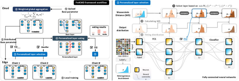
Figure 3: The framework of FedCMD with dynamic personalized layer selection.

IV-C Wasserstein Distance

The Wasserstein distance [19] is a measure used to quantify the difference between two probability distributions. It represents the minimum effort required to reshape one distribution into another. For distributions $\mu$ and $\nu$, the Wasserstein distance is defined as the lowest expected cost necessary for transforming $\mu$ into $\nu$. It is mathematically expressed as:

$$\text{W}_{p}(\mu,\nu)=\left(\inf_{\gamma\in\Gamma(\mu,\nu)}\int_{U\times V}c(\mu,\nu)^{p}\,d\gamma(\mu,\nu)\right)^{\frac{1}{p}},$$ (4)

where, $U$ and $V$ represent the spaces of the distributions $\mu$ and $\nu$. $\Gamma(\mu,\nu)$ includes all possible joint distributions that conform to the marginal distributions $\mu$ and $\nu$. The term $c(\mu,\nu)$ is the cost function measuring the distance between elements in $\mu$ and $\nu$, and $p$ indicates the order of the Wasserstein distance. This metric is widely used in areas such as data mining [28], image processing [29], and generative modeling [30].

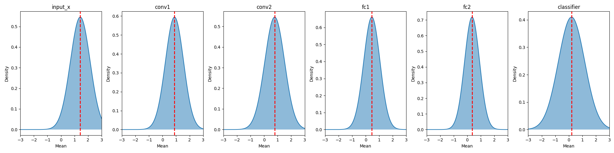
Figure 4: The feature distribution of different layers for LeNet5 [25]

V Framework with contrastive layer selection mechanism

In this section, we first present an contrastive layer selection mechanism that employs a new distance measurement based on Wasserstein distance. Then, we illustrate the FedCMD framework as applied within the Cloud-Edge system.

V-A Contrastive layer selection mechanism

Before discussing the contrastive layer selection, we introduce a new metric for distribution distance measurement, named feature distribution transfer, which is based on the Wasserstein distance, and the formulation is as follows:

$$s_{l}=\min\text{W}_{2}\left(\left(z^{o_{l}}-z^{o_{l-1}}\right),\left(z^{y}-z^{x}\right)\right),$$ (5)

where $\text{W}_{2}(\cdot)$ denotes the Wasserstein distance function with $p=2$. The terms $o_{l}$ and $o_{l-1}$ refer to the outputs of the $l$-th and $(l-1)$-th layers of the neural network, respectively. Their associated low-dimensional feature distributions of the $l$-th and $(l-1)$-th layers are denoted by $z^{o_{l}}$ and $z^{o_{l-1}}$. The variables $x$ and $y$ represent the input data sample and its corresponding label in the dataset. Their associated feature distributions are denoted by $z^{x}$ and $z^{y}$, which capture the representations of the input and label data according to the data distribution. Fig. 4, shows the Gaussian distribution of each layer’s outputs for LeNet5 model in the CIFAR-10 dataset. From this visualization, it is observable that the feature distributions of the intermediate layers are gradually shifting toward zero-mean distribution (CIFAR-10 is a class-balanced dataset). Furthermore, the extent of this shift, such as conv2 to fc1 and fc1 to fc2, is not uniform across different layers. The feature distribution transfer distance, $s_{l}$, thus quantifies the alignment of the low-dimensional feature transformations of the neural architecture from $z^{o_{l}}$ to $z^{o_{l-1}}$ with the data distribution transfer from inputs $z^{x}$ to labels $z^{y}$.

The formulation of the feature distribution transfer metric, $s_{l}$, is grounded in the principle that intermediate hidden layers of a neural network capture low-dimensional feature information. Represented by $o_{l}$ and $o_{l-1}$, these outputs embody the low-dimensional features extracted by the network. In cases where clients have heterogeneous data distributions, the low-dimensional feature information they extract also varies accordingly. To address this, we represent the low-dimensional feature distributions of the $l$-th and $(l-1)$-th layers as $z^{o_{l}}$ and $z^{o_{l-1}}$ respectively, and for simplicity, we model $z$ as a Gaussian distribution.

The rationale behind this approach is our belief that the optimal personalized layer should closely align with the unique data distribution characteristics of each client. Since $z^{x}$ and $z^{y}$ capture the heterogeneous data distribution, we constructed $s_{l}$ to evaluate this alignment. This metric quantifies how closely the neural network’s feature transformations from $z^{o_{l}}$ to $z^{o_{l-1}}$ match the shifts in data distribution from inputs $z^{x}$ to labels $z^{y}$, thus guiding the selection of the most suitable personalized layer in alignment with each client’s heterogeneous data.

Due to the black-box nature of neural networks, it is challenging to precisely compute the feature distribution transfer at each layer, hence estimation is employed. Leveraging $x$ and $y$ as references, the difference between the distribution distances of the current layer output and the original data $x$, original labels $y$, and the preceding layer output and the original data $x$, original labels $y$ is utilized as an estimate of the current layer’s feature distribution transfer. Eq. (5) can be further rewritten as:

$$s_{l} =\min\text{W}_{2}\left(\left(z^{o_{l}}-z^{o_{l-1}}\right),\left(z^{y}-z^{x}\right)\right)$$ (6)

$$\approx\min\big{|}\underbrace{\left(\text{W}_{2}\left(z^{o_{l}},z^{y}\right)-\text{W}_{2}\left(z^{o_{l}},z^{x}\right)\right)}_{\text{Prat A}}-$$

$$\underbrace{\left(\text{W}_{2}\left(z^{o_{l-1}},z^{y}\right)-\text{W}_{2}\left(z^{o_{l-1}},z^{x}\right)\right)}_{\text{Part B}}\big{|}.$$

The reason for employing the $l_{1}$ norm is that a negative value for the Wasserstein distance holds no meaningful interpretation. Part A represents the Wasserstein distance between the distribution transfer of the $l$-th layer output and the original data, while Part B represents the Wasserstein distance between the $(l-1)$-th layer output’s distribution transfer and the original data, highlighting the difference as an estimate of the $l$-th layer’s feature distribution transfer increment.

V-B FedCMD Framework

The proposed FedCMD framework is illustrated in Fig 3. We consider the Cloud-edge cooperation system, in which two types of nodes are involved, including one Cloud server, and multiple edge clients. FedCMD contains two major phases including the personalized layer selection phase and the heterogeneous federated learning phase with the Cloud-edge model decoupling. In personalized layer selection phase, the Cloud-edge system employs the standard federated learning such as FedAvg and utilizes the contrastive layer selection mechanism to collaboratively elect the personalized layer. Thus, the selection proceeds as follows:

• Global parameters broadcasting: The central server initializes the global model parameter and distributes them to all edge clients.

• Local model updating: After receiving the global parameter, each client updates their local model and trains the model using the local data.

• Local Layer Selection: Based on the criteria outlined in Eq. (6), each edge client selects a personalized layer from their model during the training.

• Communication of local gradients: Edge clients send updates of their local model parameters and their chosen personalized layer back to the Cloud server.

• Cloud-side processing: The Cloud server applies the standard federated aggregation to update the parameter of the global model and determine the layer selected by the most number of edge clients as the personalized layer.

Once this personalized layer is determined, it remains fixed throughout the heterogeneous federated learning phase. The personalized layer’s parameters do not participate in global aggregation and are updated locally on the edge client side. In contrast, the other layers of the model parameters are updated through a weighted federated aggregation, the specifics of which will be detailed in the algorithm design section. The process of the federated learning phase can be outlined as:

• Global parameters broadcasting: The central Cloud server transmits the global model parameter, excluding the personalized layer, to edge clients.

• Local model updating: Upon receiving the global parameter, each edge client updates their local model and trains the model using the local data.

• Communication of local gradients: Edge clients send updates of their local model parameters back to the Cloud server.

• Cloud-side processing: The Cloud server utilizes the personalized layer parameters to calculate the weight matrix and implements weighted federated aggregation to update the parameters of the body layers.

VI Algorithm Design

VI-A FedCMD design

FedCMD approach comprises two distinct phases: the personalized layer selection phase and the heterogeneous federated learning phase, involving three key sub-algorithms: Client-side update, Personalized layer selection, and Heterogeneous federated learning.

Input: The Cloud server paremeters $\theta_{i}^{k}$.

Output: The local model parameters $\theta_{i}^{k}$ or $(\omega_{i}^{k},\phi_{i}^{k})$ updated with local data.

1 Splits $\theta_{i}^{k}\to(\omega_{i}^{k},\phi_{i}^{k})$;

2for each local epoch do

3       Update $\theta_{i}^{k}$ or $(\omega_{i}^{k},\phi_{i}^{k})\leftarrow SGD_{i}(\omega_{i}^{k},\phi_{i}^{k};\mathcal{D}_{i})$ ;

4 end for

5return $\theta_{i}^{k}$ or $(\omega_{i}^{k},\phi_{i}^{k})$ ;

Algorithm 1 ClientUpdate($i,\theta_{i}^{k}$): // run on client i

Input: The number of current phase communication round $K_{p}$, the candidate list $\mathcal{S}$.

Output: The personalized layer $l^{*}$.

1 The Cloud Server delivers the initialization parameter $\theta_{G}^{0}$ to the edge clients;

2Calculate the mean and std of the local data and fit the distribution $z^{x}$ and $z^{y}$;

3for $k=1,\ldots,K_{p}$ do

4       /* Run on the edge clients */

5      $\mathcal{C}^{k}\leftarrow$ (random set of $n^{k}$ clients from $\mathcal{C}$);

6      for each client $i\in\mathcal{C}^{k}$ in parallel do

7             Receive $\theta_{G}^{k-1}\to\theta_{i}^{k-1}$ from the Cloud server;

8            $\theta_{i}^{k}\leftarrow$ ClientUpdate $(i,\theta_{i}^{k-1})$;

9            for each layer output $o_{l}$ do

10                   Calculate the mean and std for each layer $l$ and fit the distribution $z^{o_{l}}$ and $z^{o_{l-1}}$;

11                  Calculate $s_{l}$ by Eq. (6) and add the corresponding layer into candidate list $\mathcal{S}$;

12             end for

13            

14            Update $\theta_{i}^{k}$ to the Cloud server;

15       end for

16      

17      /* Run on the Cloud server */

18      Select the layer that appears most frequently in $\mathcal{S}$ as the personalized layer for $\mathcal{C}^{k}$, and recording it;

19      $\theta_{G}^{k}\leftarrow\sum_{i\in\mathcal{C}^{k}}\frac{|\mathcal{D}_{i}|}{|\mathcal{D}|}\theta_{i}^{k}$, where $|\mathcal{D}|=\sum_{i\in\mathcal{C}^{k}}|\mathcal{D}_{i}|$;

20      Broadcast $\theta_{G}^{k}$ to all edge clients.

21 end for

22

Select the most frequent layer in $K_{p}$ rounds as the final decision of the personalization layer $l^{*}$.

Algorithm 2 Personalized Layer Selection

Client-side updates

For each client $i$, the client model parameters $\theta_{i}^{k}$ or $(\omega_{i}^{k},\phi_{i}^{k})$ are updated using local data $\mathcal{D}_{i}$ through the stochastic gradient descent approach. The pseudocode for this process is illustrated in Algorithm 1.

Personalized Layer Selection Phase

Let the number of total communication rounds be denoted as $K$, and the number of current phase communication rounds as $K_{p}$. For each communication round, utilize Eq. (6) to compute the distribution distance between each layer’s $z^{o_{l}}-z^{o_{l-1}}$ and $z^{y}-z^{x}$. Identify the layer corresponding to the minimum distance, and then, through a voting mechanism, determine the most frequent layer to augment the candidate list $\mathcal{S}$ at round $k$. Upon completion of the final communication round in this stage, select the most recurrent layer from $S$ as the fixed personalized layer $l^{*}$ for the subsequent stage. The aggregation method for this stage follows the classical FedAvg[3] approach. See Algorithm 2 for the detailed process.

Heterogeneous Federated Learning Phase

In the stage of heterogeneous federated learning, the personalized selection outcome layer $l^{*}$, derived from the preceding phase, is intended to be employed throughout subsequent $K-K_{p}$ communication rounds. In this phase, each client personalization layer is set to $l^{*}$ and remains unchanged, $i.e.$, it is updated locally but no other layers are selected. Moreover, based on the results of personalized layer selection, a weighted parameter aggregation is applied to the model update, according to Eq. (7) and (8). Algorithm 3 shows the detailed process.

VI-B Weighted Global Aggregation

Following the personalized-layer-selection outcome $l^{*}$, the global aggregation is divided into two distinctive parts: 1) Layers preceding the personalized layer primarily emphasize feature extraction, leaning towards generality. Leveraging the sample weighting approach introduced in FedAvg [3] as Eq. (2), these layers undergo an averaging process. Conversely, 2) layers succeeding the personalized layer tend to accentuate heterogeneity, drawing inspiration from pFedSim [16]. The aggregation involves utilizing the cosine similarity of personalized layer parameters for weighted averaging, which can be calculated as follows:

$$\theta_{i}^{k}=\phi_{i}^{k}\circ\omega_{i}^{k}=\left\{\begin{aligned} &\omega_{i}^{k}=\frac{1}{\sum_{j\in\mathcal{C}^{k}}\Phi_{ij}}\sum_{j\in\mathcal{C}^{k}}\Phi_{ij}\omega_{j}^{k-1},\\ &\phi_{i}^{k}=\phi_{i}^{k-1},\end{aligned}\right.$$ (7)

where $\Phi_{ij}$ can be further written as Eq (8). Here, we define $\epsilon$ as a small positive value (we set $10^{-8}$ in our experiments) to avoid yielding extreme values. We denote $\theta_{l^{*}}(i)$ as the parameters of the selected personalized layer $\phi_{i}$ for client $i$.

$$\Phi_{ij} =\mathrm{cosine}[\theta_{l^{*}}(i),\theta_{l^{*}}(j)]$$ (8)

$$=\frac{\phi_{i}\cdot\phi_{j}}{\parallel\phi_{i}\parallel\cdot\parallel\phi_{j}\parallel+\epsilon},$$

where $\Phi_{ij}\in[0,1]$, and a higher value implies that clients $i$ and $j$ are more similar. The aggregation approach outlined in this context holds the potential for further extension into more sophisticated forms to tackle challenges across diverse scenarios. FedCMD refrains from exchanging any additional information apart from model parameters. Crucially, it preserves the personalized layer parameters, refraining them from undergoing the aggregation process. In contrast to alternative baseline methods, it showcases reduced expenses and a superior degree of privacy safeguarding.

Input: The number of total communication round $K$, number of current phase communication round $K_{p}$, the personalized layer $l^{*}$

Output: The personalized parameters of edge clients, $\{\omega_{1}^{K},\omega_{2}^{K},\ldots,\omega_{N}^{K}\}$

1 Receive $\theta_{G}^{K_{p}}$ from previous phase for all edge clients in $\mathcal{C}$ and decouple it into $\omega_{G}^{K_{p}},\phi_{G}^{K_{p}}$;

2for $k={K_{p}}+1,\ldots,K$ do

3       /* Run on the edge clients */

4      $\mathcal{C}^{k}\leftarrow$ (random set of $n^{k}$ clients) ;

5      for each client $i\in\mathcal{C}^{k}$ in parallel do

6             Receive $\omega_{G}^{k-1}\to\omega_{i}^{k-1}$ from the Cloud server;

7            Get $\theta_{i}^{k-1}\leftarrow\omega_{i}^{k-1}\circ\phi_{i}^{k-1}$;

8            $(\omega_{i}^{k},\phi_{i}^{k})\leftarrow$ ClientUpdate$(i,\theta_{i}^{k-1})$;

9            Update $(\omega_{i}^{k},\phi_{i}^{k})$ to the Cloud server;

10       end for

11      

12      /* Run on the Cloud server */

13      for two different clients $i,j\in\mathcal{C}^{k}$ do

14             Compute the similarity matrix $\Phi_{ij}$ by Eq. (8);

15       end for

16      

17      Update $\{\omega_{i}^{k}\}$ based on Eq. (7) and broadcast ge to the $i$-th edge client;

18 end for

Algorithm 3 Heterogeneous Federated Learning

VI-C Implementation and Complexity Analysis

FedCMD consists of two crucial stages: personalized layer selection and heterogeneous federated learning. In this subsection, we provide an implementation and complexity overview for each stage based on the algorithm’s description.

Firstly, we consider the client-side update, a subprocess utilized in both two phases. Assuming each stochastic gradient descent (SGD) operation is an $\mathcal{O}(1)$ process. The time complexity of the ClientUpdate algorithm focuses on two factors: the number of local epochs $E$ and the number of samples $n_{i}$ of the client $i$. Therefore, the time complexity is $\mathcal{O}(E\cdot n_{k})$.

In the edge client workflow of the personalized layer selection phase, the process starts each communication round by selecting a set of edge clients $\mathcal{C}^{k}$ from the total pool $\mathcal{C}$, which has a complexity of $\mathcal{O}(|\mathcal{C}|)$. Then, the local trains on the chosen edge clients $\mathcal{C}^{k}$ are parallel performed using the ClientUpdate. For a model comprising $L$ layers, we assume the complexity of each edge client to calculate and fit the Gaussian distribution $\{z^{o_{l}}\}$ to be $\mathcal{O}(L)$, and the Wasserstein distance computation as per Eq. (6) to be $\mathcal{O}(1)$. The complexity of this step is $\mathcal{O}(|\mathcal{C}^{k}|+E\cdot n_{k}+L+1)$. Given that $L$ is significantly smaller than both $\mathcal{C}^{k}$ and $n_{k}$, we simplify the time complexity to $\mathcal{O}(|\mathcal{C}^{k}|+E\cdot n_{k})$. On the Cloud server side, the time complexity of both each round’s personalized layer selection voting and server parameter updating is $\mathcal{O}(|\mathcal{C}^{k}|)$. Algorithm 2 repeats the above process for $K_{p}$ rounds, leading to the overall time complexity of $\mathcal{O}(K_{p}\cdot(|\mathcal{C}^{k}|+E\cdot n_{k}))$.

Finally, we analyze the time complexity of the second phase. On the edge client side, involves the model decoupling, and ClientUpdate. We consider the time complexity of model decoupling as $\mathcal{O}(1)$ and ClientUpdate is $\mathcal{O}\left(|\mathcal{C}^{k}|+E\cdot n_{k}\right)$. The time complexity on the client side is $\mathcal{O}\left(|\mathcal{C}^{k}|+E\cdot n_{k}\right)$. Moreover, there is a need to compute the cosine similarity matrix $\Phi$ between any two clients on the Cloud server. Assuming the time complexity of Eq. (8) is $\mathcal{O}(1)$. The steps from 12 to 14 of Algorithm 3 is $\mathcal{O}\left(\left|\mathcal{C}^{k}\right|^{2}\right)$. Further, the time complexity of weighted aggregation based on Eq. (7) is $\mathcal{O}\left(\left|\mathcal{C}^{k}\right|\right)$ since it provides $\{\omega_{i}^{k}\}$ for each of edge client $i$. The complexity of Algorithm 3 is $\mathcal{O}\left(\left(K-K_{p}\right)\cdot\left(\left|\mathcal{C}^{k}\right|^{2}+\left|\mathcal{C}^{k}\right|+E\cdot n_{k}\right)\right)$, which can be simplified as $\mathcal{O}\left(K\cdot\left(\left|\mathcal{C}^{k}\right|^{2}+E\cdot n_{k}\right)\right)$.

In summary, the time complexity of the FedCMD framework is governed by the number of edge clients $|\mathcal{C}^{k}|$, the size of their local datasets $n_{k}$, the number of epochs $E$, and the number of communication rounds $K$.

VII Performance Evaluation

In this section, we introduce the experimental settings, datasets, baselines, and implementation. We evaluate the performance of our solution by comparing it with nine other methods across accuracy, scalability, ablation experiment, class-wise accuracy analysis, and communication overhead.

VII-A Experiment Setup and Datasets

We build the federated learning prototype based on an open-source benchmark. All experiments are conducted on a high-performance server with GPU (NVIDIA GeForce RTX 4090 24GB) and CPU (Intel i9-13900K, 24-Core, 3.00GHz), using Pytorch 3.10.13. The code is available at repository.

Datasets

Our experiments span ten open benchmark datasets: CIFAR-10, CIFAR-100, CINIC10, EMNIST, FMNIST, MedmNistA, MedmNistC, MNIST, SVHN, and Tiny ImageNet. For further details, please refer to Appendix -A. Each dataset was divided into 100 subsets (i.e., $n=100$), following the Dirichlet distribution Dir($\alpha$) with $\alpha$ set to values within {0.1, 0.5, 1.0}, to simulate scenarios with non-IID data. The degree of non-IID is determined by $\alpha$, where a smaller $\alpha$ value indicates more significant data heterogeneity. For example, at $\alpha=0.1$, the non-IID degree is quite pronounced, suggesting that the data held by any specific client is unlikely to cover all classes (i.e., $|\mathcal{Y}_{i}|\leq|\mathcal{Y}|$), where $\mathcal{Y}_{i}$ represents the label space of data distributed to the $i$-th client.

TABLE VI: Average model accuracy over datasets for $\alpha=0.1$. Bold and underlined indicate the best and second-best respectively.

Method	CIFAR10	CIFAR100	CINIC10	EMNIST	FMNIST	MedmNistA	MedmNistC	MNIST	SVHN	T. ImageNet
Local-Only	85.356	36.058	78.876	92.712	95.528	91.808	90.077	96.555	89.402	21.424
FedAvg [3]	24.539	13.845	29.516	75.648	77.701	67.475	67.814	94.668	68.894	9.35
FedBN [23]	41.496	13.803	42.703	77.749	79.463	76.026	70.051	95.503	73.858	10.721
FedAP [24]	84.092	30.184	75.67	92.829	95.383	94.598	90.937	98.452	92.907	14.412
FedBabu [15]	29.015	5.718	23.864	73.819	74.808	64.034	66.693	94.32	67.33	3.467
FedFomo [32]	84.081	35.754	76.455	92.411	95.341	91.351	89.712	96.561	88.517	20.513
FedProx [8]	28.893	12.897	29.333	74.547	79.285	66.074	67.766	93.47	70.442	10.116
FedRep [14]	85.129	36.5	82.914	94.379	95.501	91.691	88.662	97.852	91.531	26.066
pFedSim [16]	81.712	38.452	74.771	94.552	96.171	94.113	92.594	99.062	93.371	30.179
FedDyn [31]	27.538	13.475	30.278	75.569	78.536	66.563	65.816	94.369	72.487	9.423
FedPer [21]	81.779	36.777	78.905	93.949	95.709	93.903	92.853	98.8	93.176	26.083
FedCMD	87.252	48.061	80.773	94.245	96.569	96.464	94.588	99.441	95.023	31.107

TABLE VII: Average model accuracy over datasets for $\alpha=0.5$. Bold and underlined indicate the best and second-best respectively.

	CIFAR10	CIFAR100	CINIC10	EMNIST	FMNIST	MedmNistA	MedmNistC	MNIST	SVHN	T. ImageNet
Local-Only	57.366	14.37	55.863	84.462	87.024	79.494	74.989	92.377	74.408	6.646
FedAvg [3]	44.085	17.393	41.550	82.636	84.491	81.696	77.488	96.908	82.54	10.207
FedBN [23]	50.654	16.845	46.284	82.859	84.982	85.712	81.113	97.306	83.514	11.26
FedAP [24]	62.987	18.439	56.187	86.864	89.945	90.249	87.128	98.016	87.571	6.948
FedBabu [15]	44.387	8.754	39.173	82.477	84.024	81.109	78.617	96.963	81.801	3.318
FedFomo [32]	58.419	13.3	55.029	83.659	86.611	78.381	74.932	93.385	72.33	7.951
FedProx [8]	45.004	16.33	41.051	82.07	83.582	80.56	77.806	96.781	82.273	10.64
FedRep [14]	64.459	15.594	65.658	88.551	89.622	85.346	77.669	96.606	84.967	10.325
pFedSim [16]	61.379	21.335	58.836	90.055	89.908	89.114	87.498	98.055	88.214	16.725
FedDyn [31]	43.818	16.861	40.815	82.711	84.11	81.278	77.674	97.021	82.038	10.085
FedPer [21]	61.908	16.908	62.104	88.032	90.034	88.544	87.367	97.67	87.592	10.615
FedCMD	71.331	27.531	64.409	89.596	92.26	93.982	90.735	98.636	90.039	14.561

TABLE VIII: Average model accuracy over datasets for $\alpha=1.0$. Bold and underlined indicate the best and second-best respectively.

Method	CIFAR10	CIFAR100	CINIC10	EMNIST	FMNIST	MedmNistA	MedmNistC	MNIST	SVHN	T. ImageNet
Local-Only	48.019	9.27	44.726	79.627	82.121	74.161	68.507	90.564	70.358	4.037
FedAvg [3]	45.101	17.318	42.239	83.254	84.613	86.537	82.310	96.927	82.969	10.274
FedBN [23]	47.935	16.756	44.147	83.012	84.841	87.967	83.808	97.218	84.108	11.462
FedAP [24]	56.092	15.853	47.755	83.921	86.848	90.233	86.504	97.59	87.33	5.847
FedBabu [15]	44.735	9.025	43.988	82.806	84.436	85.716	80.235	96.776	82.582	3.63
FedFomo [32]	46.625	8.84	44.022	78.865	82.282	73.107	73.981	93.311	68.423	5.376
FedProx [8]	44.853	16.665	43.028	82.443	84.515	86.496	82.333	96.88	82.792	10.637
FedRep [14]	55.345	10.167	57.861	84.444	86.088	83.942	74.709	95.976	84.163	6.77
pFedSim [16]	56.454	17.055	52.834	87.203	88.276	88.296	86.434	97.587	87.828	12.905
FedDyn [31]	45.964	17.016	42.826	83.217	84.754	86.851	82.584	97.042	83.229	10.271
FedPer [21]	56.753	12.477	55.777	84.258	88.018	87.846	85.892	97.198	87.066	7.91
FedCMD	64.508	22.178	57.468	86.454	89.837	93.312	89.448	98.271	89.464	12.537

Baselines

We compare FedCMD with nine state-of-the-art federated learning solutions. To create a baseline for evaluating the generalization and personalization performance, respectively, we implement FedAvg [3] and Local-training-only in our experiments. Local-training-only means that the clients only update parameters with their local data without the global parameter aggregation. In addition, we achieved baseline comparisons of the following 9 algorithms, and see Appendix -A for detailed hyper-parameter settings:

• FedProx [8] adds a proximal term to the loss function to prevent the edge client model from drifting away from the global model.

• FedRep [14] treats the classifier as the personalized layer, and trains the classifier locally and the feature extractor sequentially.

• FedBabu [15] initializes randomly the classification header and updates the body only during training.

• pFedSim [16] uses classifier distance as the weights for global aggregation and based on model decoupling.

• FedPer [21] employs the last-layer-as-head decoupling by splitting the network into the base and personalized layer to achieve personalization.

• FedBN [23] preserves batch normalization layers in the edge client model locally to stabilize training and the rest uploads to aggregate.

• FedAP [24] measures client-wised similarity using Wasserstein distance based on statistics from the batch normalization layer to optimize model aggregation.

• FedDyn [31] aligns the solutions of each edge client and server utilizing a dynamic regularizer from a communication perspective.

• FedFomo [32] calculates how much one client can benefit from the other, deriving the optimally weighted model combination for each client.

Implementation

We implemented LeNet5 [25] for all methods to conduct performance evaluation on all datasets. According to the setup in [16], we evenly split the dataset of each edge client into the training and test sets with no intersection, i.e., $|\mathcal{D}_{i}^{train}|=|\mathcal{D}_{i}^{test}|$. On the edge client side, we adopt SGD as the local optimizer. The local learning rate is set to 0.01 for all experiments. All experiments shared the same join ratio $\gamma$ equals to 0.1, communication round $K=200$, local epoch $E=5$, and batch size equals to 32. In Appendix -A, we provide the list of the model architectures and the full hyperparameter configurations employed in the methods involved.

VII-B Comparison of Classification Accuracy

We compare the average model accuracy performance of our solution with other baselines in Table VI–VIII. The results displayed in Table VI compare the average accuracy with $\alpha=0.1$, where FedCMD exhibits outstanding performance across most datasets. Notably, FedCMD leads with significant margins in complex datasets like CIFAR100 and Tiny ImageNet, with remarkable accuracy improvements of 9.609% and 0.928% respectively over the second-best results. Compared to established methods like FedBN, FedBabu, FedProx and FedDyn, FedCMD shows a marked improvement. For example, in the CIFAR10 dataset, our solution achieves an accuracy of 87.252%, which is 1.896% higher than the second-best, Local-Only. Similarly, in MedmNistC, our solution attains 94.588%, outperforming the nearest competitor, FedPer, by 1.735%. The underlined results indicate the second-best performing methods, which offer strong competition in datasets like CINIC10. For instance, FedRep demonstrates robust performance in CINIC10 with an accuracy of 82.914%. These results suggest that while other methods have merits in specific conditions, FedCMD consistently leads in adapting to non-IID data in most federated learning environments.

In Table VII, we see average accuracy with $\alpha=0.5$, indicating less data heterogeneity compared to $\alpha=0.1$. In this context, the performance of our FedCMD method, while still leading in many cases. Despite this, FedCMD remains the top performer in several datasets, notably achieving the highest accuracy in CIFAR10 at 71.331%, which is 6.872% higher than the second-best, FedRep. In CIFAR100, FedCMD leads with 27.531%, outperforming pFedSim, the second-best, by a significant margin of 6.196%. This trend continues in Tiny ImageNet, where FedCMD’s accuracy of 14.561% is second only to pFedSim’s 16.725%. Compared with other methods, our solution’s performance in datasets like FMNIST and MedmNistA is notably superior, with accuracy of 92.260% and 93.982% respectively, demonstrating its effectiveness even in less heterogeneous settings. Despite the reduced heterogeneity, our solution continues to demonstrate robust performance across ten datasets with $\alpha=0.5$.

Table VIII shows the average model accuracy with $\alpha=1.0$, indicating a more uniform data distribution than $\alpha=0.1$ and $\alpha=0.5$. Despite this, FedCMD continues to lead in several datasets. Notably, it achieves the highest accuracy in CIFAR10 at 64.508%, surpassing the second-best FedPer by 7.755%. In CIFAR100, FedCMD tops the list with an accuracy of 22.178%, showing a noticeable improvement over FedAvg. In datasets like FMNIST and MedmNistA, our solution outperforms others with the accuracy of 89.837% and 93.312%, respectively, underlining its effectiveness across varied settings. FedCMD also demonstrates strong performance in Tiny ImageNet, achieving 12.537%, which, although not the highest, is close to the top performer, pFedSim. Compared to FedDyn, our solution shows a considerable advantage in datasets like CIFAR10 and CIFAR100, but a narrower lead in more uniform datasets like EMNIST and MNIST. Overall, while FedCMD’s performance advantage diminishes in less heterogeneous scenarios ($\alpha=1.0$), it still shows notable effectiveness and robustness across a range of datasets.

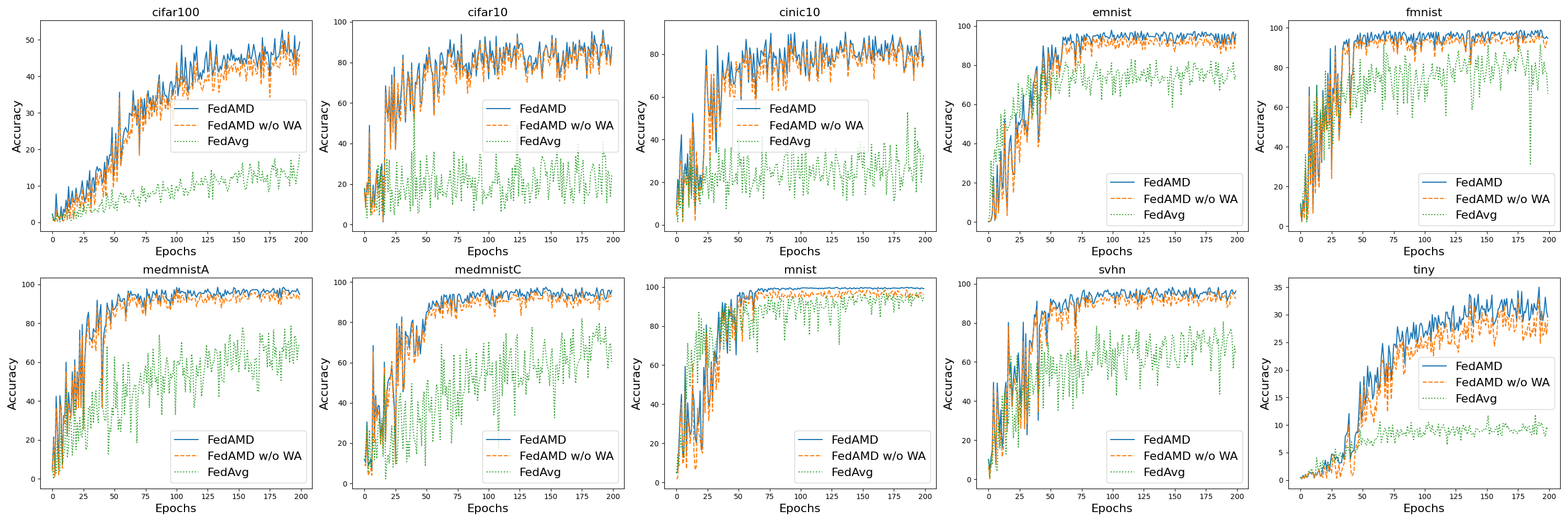
Figure 5: Accuracy comparison of FedCMD, FedCMD without weighted aggregation, and original FedAvg across ten datasets.

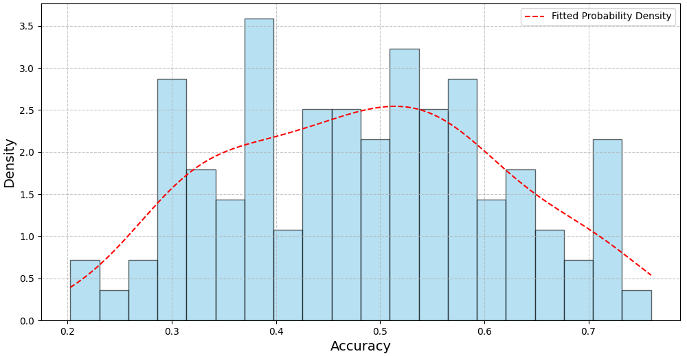
Figure 6: Probability Density Function of Accuracy on CIFAR100.

VII-C Class-wise Accuracy Analysis

Fig. 6 shows the probability density function of class-wise accuracy on CIFAR100 with FedCMD. CIFAR100 consists of 100 distinct classes, and this analysis involves calculating the accuracy for each individual class. The probability density histogram in the figure is based on these 100 accuracy values, along with a fitted probability density curve to visualize the distribution pattern. From the histogram, it’s evident that the accuracy distribution for the 100 classes lies within the range of 20% to 75%. A significant concentration of class accuracies is observed around 50%, indicating a median level of recognition capability for most classes. However, the graph also reveals the presence of a few classes with notably lower accuracy, below 30%, as well as some with higher accuracy, exceeding 70%. This distribution suggests a varied level of difficulty in accurately recognizing different classes within CIFAR100. While a majority of the classes are recognized with moderate accuracy, a subset of classes poses greater challenges or are recognized with high accuracy.

VII-D Ablation Experiment

As illustrated in Fig. 5, we present the results of our ablation experiments. These experiments compare three designs: FedCMD (which includes both weighted aggregation and model decoupling), FedCMD without weighted aggregation (employing only model decoupling), and the original FedAvg method that doesn’t utilize either weighted aggregation or model decoupling. The comparison between FedCMD and FedCMD without weighted aggregation reveals that the inclusion of weighted aggregation in FedCMD contributes to a modest performance enhancement, with an average improvement of approximately 2% across all ten scenarios. However, the most significant performance leap is observed when comparing FedCMD without weighted aggregation to the original FedAvg. The absence of model decoupling and weighted aggregation in FedAvg leads to substantially lower performance. For instance, in the CIFAR10 dataset, the implementation of model decoupling in FedCMD without weighted aggregation results in nearly a 60% increase in accuracy. Even in the MNIST dataset, there’s at least a 3% improvement in performance. These results show the importance of model decoupling in the performance enhancement.

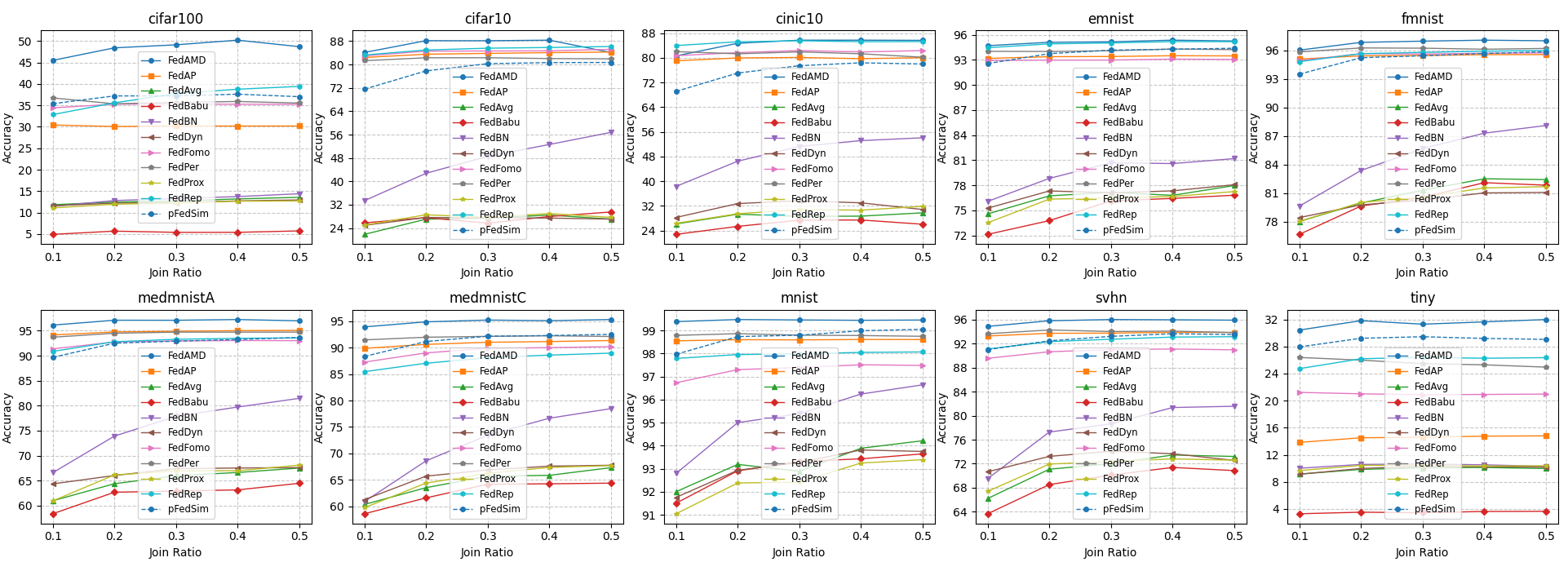
Figure 7: Accuracy comparison for FedCMD and ten solutions (including FedAvg) with different join ratios across ten datasets.

VII-E Comparison of Scalability

As shown in Fig. 7, the performance of various federated learning, including our FedCMD, was evaluated under different client join ratios {0.1, 0.2, 0.3, 0.4, 0.5}. Our FedCMD method consistently showed performance improvement with increasing join ratios in most of the datasets, such as in CIFAR-10, starting from 84.114% at a ratio of 0.1 and peaking at 88.331% at a ratio of 0.4. This trend indicates that FedCMD effectively leverages increased client participation, enhancing its performance. Comparatively, other methods like FedBN, pFedSim, and FedAP also exhibited performance boosts with higher join ratios, but none matched the level of improvement seen with FedCMD. For instance, in CIFAR-10, FedBN’s accuracy improved from 33.388% to 52.618%, and pFedSim increased from 71.559% to 80.653%. FedAP showed a consistent rise from 82.404% to 84.065%. Methods like FedBabu, FedProx, and FedDyn, however, demonstrated relatively minor improvements or fluctuations across different join ratios. FedBabu’s performance fluctuated around the mid-20% range, while FedProx and FedDyn hovered around the high-20% to low-30% range. FedFomo, FedRep, and FedPer also displayed improvements with increasing join ratios, but their increments were not as substantial as FedCMD. For example, in CIFAR-10, FedFomo and FedRep started at 82.942% and 83.257% at a ratio of 0.1, respectively, and increased to around 84.680% and 85.822% at a ratio of 0.4. Interestingly, FedBabu’s performance improves with an increase in the joining ratio but declines at the highest ratio of 0.5, suggesting a threshold beyond which more client participation does not benefit. Overall, the data demonstrates that our FedCMD method not only starts off with higher accuracy at lower join ratios but also scales more effectively with increased client participation compared to other methods.

VII-F Disscussion of Layer Selection Phase

Our study on the impact of communication rounds for the personalized layer selection phase in FedCMD reveals the relationship between the number of rounds and model accuracy. The data from Table IX shows that while most datasets benefit from an increased number of rounds, there are exceptions where fewer rounds also yield better results. In most cases, a trend of increasing accuracy with more communication rounds is evident. For instance, CIFAR10 peaks at 87.51% with 80 rounds, FMNIST reaches 96.775% with 100 rounds, and Tiny ImageNet consistently improves, achieving its highest accuracy of 31.602% with 100 rounds. This trend suggests that more communication rounds generally lead to more accurate personalized layers, enhancing overall model performance. However, some datasets such as EMNIST peak at 94.912% with just 20 rounds, indicating that fewer rounds can be more effective in certain scenarios. Similarly, CIFAR100 and MedmNistC show optimal performances at 40 rounds with an accuracy of 47.954% and 94.745%, respectively. These exceptions highlight that the relationship between communication rounds and accuracy is not always linear and can vary depending on the dataset’s characteristics. Overall, while the general trend suggests that more communication rounds in FedCMD lead to better accuracy, the optimal number of rounds is highly dataset-dependent.

TABLE IX: Accuracy with different rounds of layer selection phase across ten datasets.

Number of rounds	20	40	60	80	100
CIFAR10	84.076	87.427	87.422	87.51	87.117
CIFAR100	42.224	47.954	47.552	47.374	47.527
CINIC10	78.426	80.619	79.959	79.823	79.573
EMNIST	94.912	94.221	94.225	94.165	94.295
FMNIST	94.736	96.516	96.705	96.508	96.775
MedmNistA	95.204	96.362	96.517	96.418	96.444
MedmNistC	94.364	94.745	94.49	94.485	94.564
MNIST	99.266	99.289	99.313	99.281	99.259
SVHN	94.302	95.178	95.047	94.961	94.925
Tiny ImageNet	28.877	31.17	31.498	31.494	31.602

VII-G Communication Overhead

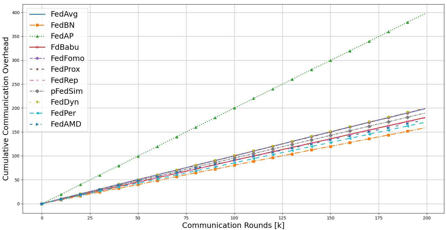
Figure 8: Comparison of Cumulative Communication Overhead.

The experimental results depicted in Fig. 8 present a comparison of the cumulative communication overhead across ten different algorithms against the benchmark FedAvg. The analysis reveals that most methods, except for FedAP, have comparable or even lower communication overhead compared to FedAvg. Notably, FedBN exhibits the lowest overhead among all. This efficiency is attributed to its approach of updating multiple layers only at the edge, eliminating the need for uploading a substantial amount of parameters to the cloud for aggregation. Similarly, FedPer also shows commendable performance due to its strategy for selecting multiple layers as personalizing. FedCMD only ranks behind FedBN and FedPer. Since the last layer typically has fewer parameters than other fully connected layers, methods fixing the last layer for personalization inherently have higher communication costs than FedCMD. In summary, our FedCMD method demonstrates effective communication overhead management.

VIII Conclusions

In this paper, we present a novel personalized layer selection in federated learning through our novel FedCMD framework. This approach challenges the conventional rigidity of existing layer-selection methods by introducing a distribution distance metric, named feature distribution shift, based on the Wasserstein distance. This metric assesses the alignment between each layer’s feature distribution and the heterogeneous data distribution of client models. To our knowledge, our work marks a significant first step in this area, offering a unique perspective on contrastive layer selection. The extensive experimental testing across ten datasets not only validates the effectiveness of our proposed metric but also demonstrates the superior performance of the FedCMD framework compared to nine other SOTA solutions. Moreover, FedCMD two-phase structure, encompassing personalized layer selection and heterogeneous federated learning, along with the introduction of practical algorithms for contrastive layer selection and weighted global aggregation. Our comprehensive exploration and analysis in this paper pave the way for future advancements in contrastive and heterogeneous federated learning.

Xingyan Chen received the Ph. D degree in computer technology from Beijing University of Posts and Telecommunications (BUPT), in 2021. He is currently a lecturer with the School of Economic Information Engineering, Southwestern University of Finance and Economics, Chengdu. He has published papers in well-archived international journals and proceedings, such as the IEEE Transactions on Mobile Computing, IEEE Transactions on Circuits and Systems for Video Technology, IEEE Transactions on Industrial Informatics, and IEEE INFOCOM etc. His research interests include Multimedia Communications, Multi-agent Reinforcement Learning and Stochastic Optimization.

Tian Du received her B.S. degree in Management from Huaqiao University in 2021, and currently pursuing a Ph.D. in Management specializing in Big Data Management at Southwestern University of Finance and Economics. Her research interests encompass Federated Learning, Reinforcement Learning and Time Series Clustering. She has published in relevant SCI journals. Passionate about exploring cutting-edge data management methodologies and technologies, she is dedicated to addressing intricate challenges related to Big Data, thereby contributing to the advancement of the field of Data Science.

Mu Wang received his M.S. and Ph.D. degrees in computer technology from Beijing University of Posts and Telecommunications (BUPT) in 2015 and 2020. He was a Joint Ph.D. student at the School of Electrical, Computer, and Energy Engineering (ECEE), Arizona State University. He is currently a postdoctoral research associate with the Department of Computer Science and Technology & BNRist, Tsinghua University. His research interests include information-centric networking, wireless communications, and multimedia delivery in wireless networks.

Tiancheng Gu received his B.S. degree in Engineering from Chongqing University of Posts and Telecommunications in 2023, is currently pursuing a M.S. degree in Computer Science and Technology at Southwestern University of Finance and Economics. His research primarily focuses on large-scale model inference engineering, exploring data analysis and prediction, with a particular emphasis on federated learning and data privacy protection. His career objective is to optimize large-scale model inference techniques based on inference engineering, enhancing data processing efficiency, and contributing to the field of computer science.

Yu Zhao received the B.S. degree from Southwest Jiaotong University in 2006, and the M.S. and Ph.D. degrees from the Beijing University of Posts and Telecommunications in 2011 and 2017, respectively. He is a Professor at the Southwestern University of Finance and Economics. His current research interests include natural language processing, large language models, graph learning, and fintech. He has authored more than 30 papers including IEEE TKDE, IEEE TNNLS, IEEE TMC, IEEE TMM, ACL, ICME, etc.

Gang Kou is a Distinguished Professor of Chang Jiang Scholars Program in Southwestern University of Finance and Economics, managing editor of International Journal of Information Technology & Decision Making (SCI) and managing editor-in-chief of Financial Innovation (SSCI). He is also editors for other journals, such as: Decision Support Systems, and European Journal of Operational Research. Previously, he was a professor of School of Management and Economics, University of Electronic Science and Technology of China, and a research scientist in Thomson Co., R & D. He received his Ph.D. in Information Technology from the College of Information Science & Technology, Univ. of Nebraska at Omaha; Master degree in Dept of Computer Science, Univ. of Nebraska at Omaha; and B.S. degree in Department of Physics, Tsinghua University, China. He has published more than 100 papers in various peer-reviewed journals. Gang Kou’s h-index is 57 and his papers have been cited for more than 10000 times. He is listed as the Highly Cited Researcher by Clarivate Analytics (Web of Science).

Changqiao Xu [SM’15] received the Ph.D. degree from the Institute of Software, Chinese Academy of Sciences (ISCAS) in Jan. 2009. He was an Assistant Research Fellow and R&D Project Manager in ISCAS from 2002 to 2007. He was a researcher at Athlone Institute of Technology and Joint PhD at Dublin City University, Ireland during 2007-2009. He joined Beijing University of Posts and Telecommunications (BUPT), Beijing, China, in Dec. 2009. Currently, he is a full Professor with the State Key Laboratory of Networking and Switching Technology, and Director of the Network Architecture Research Center at BUPT. His research interests include Future Internet Technology, Mobile Networking, Multimedia Communications, and Network Security. He has published over 160 technical papers in prestigious international journals and conferences, including IEEE Comm. Surveys & Tutorials, IEEE Wireless Comm., IEEE Comm. Magazine, IEEE/ACM ToN, IEEE TMC etc. He has served a number of international conferences and workshops as a Co-Chair and Technical Program Committee member. He is currently serving as the Editorin-Chief of Transactions on Emerging Telecommunications Technologies (Wiley). He is Senior member of IEEE.

Dapeng Oliver Wu [S’98-M’04-SM’06-F’13] received a B.E. degree in electrical engineering from Huazhong University of Science and Technology,Wuhan, China in 1990, an M.E. degree in electrical engineering from Beijing University of Posts and Telecommunications, Beijing, China in 1997, and a Ph.D. degree in electrical and computer engineering from Carnegie Mellon University, Pittsburgh, PA in 2003. He is currently Yeung Kin Man Chair Professor of Network Science, and Chair Professor of Data Engineering at the Department of Computer Science, City University of Hong Kong. Previously, he was on the faculty of University of Florida, Gainesville, FL, USA and was the director of NSF Center for Big Learning, USA. His research interests are in the areas of networking, communications, signal processing, computer vision, machine learning, smart grid, and information and network security. He has served as Editor in Chief of IEEE Transactions on Network Science and Engineering, Editor-at-Large for IEEE Open Journal of the Communications Society, founding Editor-in-Chief of Journal of Advances in Multimedia, and Associate Editor for IEEE Transactions on Cloud Computing, IEEE Transactions on Communications, IEEE Transactions on Signal and Information Processing over Networks, IEEE Signal Processing Magazine, IEEE Transactions on Circuits and Systems for Video Technology, IEEE Transactions on Wireless Communications and IEEE Transactions on Vehicular Technology. He is an IEEE Fellow.

-A Experiment Details

-A1 Computing Configuration

We implement our experiments using PyTorch 2.1.0+cu121 and run all experiments on Microsoft Windows 11 Professional Edition. Our system configuration includes a 13th Gen Intel(R) Core(TM) i9-13900K CPU @ 3.00GHz with 24 cores and 32 logical processors, combined with an NVIDIA GeForce RTX 4090 GPU. The system is built on a Micro-Star International Co., Ltd. MS-7D25 model (PRO Z690-A WIFI DDR4) with 64.0 GB of RAM.

-A2 Datasets Details

Dataset	Samples	Classes	Description	Resolution	Year
CIFAR10/100	60,000	10/100	Images in 10/100 classes including airplanes, cars, birds, etc.	$32\times 32$	2009
CINIC10	270,000	10	Images in 10 classes including airplanes, cars, birds, etc.	$32\times 32$	2018
EMNIST	805,263	62	Extended MNIST with letters and digits	$28\times 28$	2017
FMNIST	70,000	10	Fashion item images	$28\times 28$	2017
MNIST	70000	10	Handwritten digits	$28\times 28$	1998
MedmNistA/C	58,850/23,600	11	Biomedical images on abdominal CT.	$28\times 28$	2019
SVHN	600,000	10	Street view house numbers	$32\times 32$	2011
Tiny ImageNet	110,000	200	Tiny ImageNet dataset	$64\times 64$	2015

TABLE X: Statistical information of used datasets on clients.

The foundational information pertaining to the datasets employed in our experiments is delineated in Table X. In order to ensure equitable comparisons across different methodologies, we adhere to the configuration established in pFedSim. This involves the segmentation of each dataset into 100 subsets, effectively constituting 100 clients. It is essential to note that the data distribution throughout the experiments is held constant, thus providing a consistent basis for evaluating the efficacy of diverse methods.

-A3 Model Architecture

LeNet5 [25] serves as the backbone model in our experiments. The detailed architectures and the two extended architectures are illustrated in Table XI-Table XIII, encompassing the layers with abbreviations in the PyTorch style.

Component	Layer
Feature Extractor	Conv2D (in=3, out=6, kernel=5, stride=1, pad=0)
	Conv2D (in=3, out=16, kernel=5, stride=1, pad=0)
	MaxPool2D (kernel=2, stride=2)
	Flatten()
	FC (out=120)
	FC (out=84)
Classifier	FC (out=num_classes)

TABLE XI: LeNet5 Architecture. Conv2D() consists of a 2D convolution layer, batch normalization layer, and ReLU activation, which is executed sequentially. The in, out, kernel, stride, pad represent the input channel, output channel, kernel size, convolution kernel step size moving, padding size, respectively; MaxPool2D() is a max pooling layer for 2D input; Flatten() is for reshaping input from 2D to 1D; FC() is a fully connected layer, out means the number of features output has.

Component	Layer
Feature Extractor	Conv2D (in=3, out=6, kernel=5, stride=1, pad=0)
	Conv2D (in=3, out=16, kernel=5, stride=1, pad=0)
	MaxPool2D (kernel=2, stride=2)
	Flatten()
	FC (out=120)
Classifier	FC (out=num_classes)

TABLE XII: Extended LeNet5 Architecture 1. Conv2D() consists of a 2D convolution layer, batch normalization layer, and ReLU activation, which is executed sequentially. The in, out, kernel, stride, pad represent the input channel, output channel, kernel size, convolution kernel step size moving, padding size, respectively; MaxPool2D() is a max pooling layer for 2D input; Flatten() is for reshaping input from 2D to 1D; FC() is a fully connected layer, out means the number of features output has.

Component	Layer
Feature Extractor	Conv2D (in=3, out=6, kernel=5, stride=1, pad=0)
	Conv2D (in=3, out=16, kernel=5, stride=1, pad=0)
	MaxPool2D (kernel=2, stride=2)
	Flatten()
	FC (out=120)
	FC (out=84)
	FC (out=64)
Classifier	FC (out=num_classes)

TABLE XIII: Extended LeNet5 Architecture 2. Conv2D() consists of a 2D convolution layer, batch normalization layer, and ReLU activation, which is executed sequentially. The in, out, kernel, stride, pad represent the input channel, output channel, kernel size, convolution kernel step size moving, padding size, respectively; MaxPool2D() is a max pooling layer for 2D input; Flatten() is for reshaping input from 2D to 1D; FC() is a fully connected layer, out means the number of features output has.

-A4 Full Hyperparameter settings

We provid a comprehensive list of hyperparameter settings for all the comparative methods mentioned above. The majority of baseline hyperparameters align with the values specified in their own papers.

• FedProx [8] We set $\mu=1$.

• FedRep [14] We set the epoch for training feature extractor part to 1.

• pFedSim [16] We set the generalization ratio $\rho_{general}=0.5$.

• FedAP [24] We set model momentum $\mu=0.5$.

• FedDyn [31] We set $\alpha=0.01$.

• FedFomo [32] We set the M = 5 and the ratio of validation set to 0.2.

• FedCMD (Ours) We set the devision ratio $\rho=0.1$.

References

- [1] Z. Xu et al., “Age-Aware Data Selection and Aggregator Placement for Timely Federated Continual Learning in Mobile Edge Computing,” IEEE Transactions on Computers, pages: 1-14, 2023.
- [2] R. Zhang, Z. Xie, D. Yu, W. Liang and X. Cheng, “Digital Twin-Assisted Federated Learning Service Provisioning Over Mobile Edge Networks,” IEEE Transactions on Computers, pages: 1-13, 2023.
- [3] B. McMahan, E. Moore, D. Ramage, et al., “Communication-efficient learning of deep networks from decentralized data,” in Artificial intelligence and statistics, PMLR, pp. 1273–1282, 2017.
- [4] J. Lu, Y. Yao, J. Zhang, et al., “Soft: Softmax-free transformer with linear complexity,” in Advances in Neural Information Processing Systems, vol. 34, pp. 21297–21309, 2021.
- [5] J. Zhang, S. Guo, J. Guo, D. Zeng, J. Zhou and A. Y. Zomaya, “Towards Data-Independent Knowledge Transfer in Model-Heterogeneous Federated Learning,” IEEE Transactions on Computers, vol. 72, no. 10, pp. 2888-2901, 2023.
- [6] Y. Chen, W. Lu, X. Qin, et al., “Metafed: Federated learning among federations with cyclic knowledge distillation for personalized healthcare,” IEEE Transactions on Neural Networks and Learning Systems, pp. 1–12, 2023.
- [7] D. Yao et al., “FedGKD: Toward Heterogeneous Federated Learning via Global Knowledge Distillation,” IEEE Transactions on Computers, vol. 73, no. 1, pp. 3-17, 2024.
- [8] T. Li, A. Sahu, M. Zaheer, et al., “Federated optimization in heterogeneous networks,” Proceedings of Machine learning and systems, vol. 2, pp. 429–450, 2020.
- [9] C. T Dinh, N. Tran and J. Nguyen, “Personalized federated learning with moreau envelopes,” Advances in Neural Information Processing Systems, vol. 33, pp. 21394–21405, 2020.
- [10] T. Li, S. Hu, A. Beirami, et al., “Ditto: Fair and robust federated learning through personalization,” International Conference on Machine Learning, PMLR, vol. 33, pp. 6357–6368, 2021.
- [11] F. Sattler, K. R. Müller, W. Samek, et al., “Clustered federated learning: Model-agnostic distributed multitask optimization under privacy constraints,” IEEE transactions on neural networks and learning systems, vol. 32, no. 8, pp. 3710–3722, 2020.
- [12] G. Long, M. Xie, T. Shen, et al., “Multi-center federated learning: clients clustering for better personalization,” World Wide Web, vol. 26, no. 1, pp. 481–500, 2023.
- [13] L. Yang, J. Huang, W. Lin, et al., “Personalized federated learning on non-IID data via group-based meta-learning,” ACM Transactions on Knowledge Discovery from Data, vol. 17, no. 4, pp. 1–20, 2023.
- [14] C. Liam, H. Hamed, M. Aryan, et al., “Exploiting Shared Representations for Personalized Federated Learning,” International conference on machine learning, vol. 139, pp. 2089–2099, 2021.
- [15] J. Oh, S. Kim, S.-Y. Yun, “Fedbabu: Towards enhanced representation for federated image classification,” International Conference on Learning Representations, 2021.
- [16] J. Tan, Y. Zhou, G. Liu, et al., “pFedSim: Similarity-Aware Model Aggregation Towards Personalized Federated Learning,” arXiv preprint arXiv:2305.15706, 2023.
- [17] P. P. Liang, T. Liu, L. Ziyin, et al., “Think Locally, Act Globally: Federated Learning with Local and Global Representations,” International Workshop on Federated Learning for User Privacy and Data Confidentiality in Conjunction with NeurIPS 2019, 2019.
- [18] L. Mi, C. Fei, H. Dapeng, et al., “No Fear of Heterogeneity: Classifier Calibration for Federated Learning with Non-IID Data,” Advances in Neural Information Processing Systems, vol. 34, pp. 5972–5984, 2021.
- [19] Rüschendorf, Ludger. “The Wasserstein distance and approximation theorems.” Probability Theory and Related Fields 70.1 (1985): 117-129.
- [20] C. He, E. Ceyani, K. Balasubramanian, et al., “Spreadgnn: Decentralized multi-task federated learning for graph neural networks on molecular data,” Proceedings of the AAAI Conference on Artificial Intelligence, vol. 36, no. 6, pp. 6865–6873, 2022.
- [21] M. Arivazhagan, V. Aggarwal, A. Singh, et al., “Federated learning with personalization layers,” arXiv preprint arXiv:1912.00818, 2019.
- [22] W. Zhuang, Y. Wen, X. Zhang, et al., “Performance Optimization of Federated Person Re-Identification via Benchmark Analysis,” Proceedings of the 28th ACM International Conference on Multimedia, no. 9, pp. 955–963, 2020.
- [23] X. Li, M. Jiang, X. Zhang, et al., “FedBN: Federated learning on non-iid features via local batch normalization,” International Conference on Learning Representations, 2021.
- [24] W. Lu, J. Wang, Y. Chen, et al., “Personalized federated learning with contrastive batchnorm for healthcare,” IEEE Transactions on Big Data, pp. 1–1, 2022.
- [25] Y. LeCun, L. Bottou, Y. Bengio, et al., “Gradient-based learning applied to document recognition,” Proceedings of the IEEE, vol. 86, no. 11, pp. 2278–2324, 1998.
- [26] H. Zhu, Y. Fan, and Z. Xie, “Federated Two Stage Decoupling With contrastive Personalization Layers,” arXiv preprint arXiv:2308.15821, 2023.
- [27] R. Su, X. Pang, H. Wang, “A novel parameter decoupling approach of personalised federated learning for image analysis,” IET Computer Vision, 2023.
- [28] J. Bigot, “Statistical data analysis in the Wasserstein space,” ESAIM: Proceedings and Surveys, 2020, 68: 1-19.
- [29] She, Qingshan, et al. “Improved Domain Adaptation Network Based on Wasserstein Distance for Motor Imagery EEG Classification.” IEEE Transactions on Neural Systems and Rehabilitation Engineering 31 (2023): 1137-1148.
- [30] H. Lee, J. Lu, and Y. Tan, “Convergence of score-based generative modeling for general data distributions”, International Conference on Algorithmic Learning Theory, pp. 946-985, 2023.
- [31] A. E. A. Durmus, Z. Yue, M. Ramon, et al., “Federated Learning Based on Dynamic Regularization,” International Conference on Learning Representations, 2021.
- [32] M. Zhang, K. Sapra, S. Fidler, et al., “Personalized federated learning with first order model optimization,” International Conference on Learning Representations, 2020.
- [33] T. Maintainers, et al., “TorchVision: PyTorch’s computer vision library”, November 2016.