Proof of the nonintegrability of the PXP model and general spin-$1/2$ systems

Abstract

We propose a general framework for proving non-integrability of the quantum systems. For spin-$1/2$ systems, we show that the presence or absence of the local conserved quantity can be shown using the graph theoretical analysis. This approach helps to systematically classify the number of local conserved quantity, as aiding the proof of non-integrability of the Hamiltonian. Using this approach, we prove for the first time that the PXP model is nonintegrable. We also show that our method is applicable to the well-known proof of the non-integrability of other spin-$1/2$ systems. Our new approach offers a significant simplification of the proof for non-integrability and provides a deeper understanding of quantum dynamics.

I Introduction

Integrability is a fundamental concept in quantum systems. It refers to the ability to express certain quantities such as conserved quantities or observables, as integrals of motion. The integrable systems contain infinitely-many local conserved quantities to fully determine the dynamics and lack quantum thermalization. It has many practical implications in various areas including condensed matter physics, quantum field theory and quantum computation.Rigol et al. (2007); Pozsgay (2013); Vidmar and Rigol (2016); Andrei (1980); Zamolodchikov and Zamolodchikov (1978); Coleman (1975); Faddeev (1982); Zhang et al. (2005) From the generalization of the Bethe ansatz study showing the integrability of antiferromagnetic Heisenberg modelBethe (1931), the Yang-Baxter equationsYang (1967); Baxter (1978, 2016) and the quantum inverse scattering methodTakhtadzhan and Faddeev (1979) were developed, and these are now the main tools for studying the integrability of quantum systems. Several quantum systems including $XYZ$ modelBaxter (1972); Takhtadzhan and Faddeev (1979); Nozawa and Fukai (2020), 1-dimensional Hubbard modelShastry (1986); Fukai (2023), and the golden chain model with Fibonacci anyonsFeiguin et al. (2007) are shown to be integrable using these methods.

However, there are only few studies that deal with the non-integrability of a particular Hamiltonian, i.e. there is no local conserved quantity in the system. Therefore, in most cases, except for those specially known as integrable systems, it is difficult to determine whether the system is integrable or not. At present, the investigation of level statistics is the most general approach to distinguishing between integrable and non-integrable models: if it follows the Poisson distribution, we conclude the system is integrable, whereas if it follows the Wigner-Dyson distribution, the system is considered to be non-integrableCasati et al. (1985). However, this statement is a conjecture that has not yet been proven, and it also requires a large enough system size to be able to show the trend of the level statistics, and therefore is sometimes controversial. There exists another conjectureGrabowski and Mathieu (1995) claiming that the non-existence of the three site support conserved quantity $Q_{3}$ implies the nonintegrability of the system. Although this is easier to check than the level statistics, it is also unproven, and the argument is based on the Yang-Baxter equation, which is still unknown as a necessary condition for integrability.

Recently, Ref.[21] discusses the rigorous proof of the non-integrability of the $XYZ$ chain in the presence of magnetic field. This work sheds light on the analytic approach to the non-integrable systems. Following this method, it has been shown that another spin model, a mixed-field Ising chain model, is non-integrableChiba (2024). The system without any conserved quantity thermalizes in a long time limit to the Gibbs ensemble, while the integrable systems do not due to its extensively many conserved quantities. Thus, finding out the conserved quantities of a given Hamiltonian is a key tool to understand the dynamics of the Hamiltonian.

In this paper, we propose a new way to prove the non-integrability of the spin-$1/2$ quantum systems, adopting the graph theoretical approach. Although some details should be checked on each model, the graph theoretical approach provides the way to systematically classify the conserved quantities and thus allows us to simplify the analysis to prove the non-integrability of the systems. We exemplify the one-dimensional PXP model and prove it’s non-integrability, showing the absence of any local conserved quantities.

The PXP model is well known to describe the Rydberg atom systems with the Rydberg blockade. This model has been studied extensively in many contexts, including the quantum many-body scar (QMBS). It has been shown both experimentallyBernien et al. (2017) and theoreticallyTurner et al. (2018) that while most of the initial product thermalizes in a long time limit, a small number of initial product states shows a short time revival, which is a strong evidence of QMBSAlhambra et al. (2020). Because every initial product state thermalizes in non-integrable system while every initial product state shows a short time revival in integrable system, QMBS system can be considered as an intermediate system between non-integrable (with no local conserved quantities) and integrable (with extensively many local conserved quantities) system. Due to its exotic behavior, QMBS systems such as PXP model, its modificationsBull et al. (2020); Bluvstein et al. (2021); Su et al. (2023); Desaules et al. (2024), or other similar modelsSchecter and Iadecola (2019); Mark et al. (2020); Iadecola and Schecter (2020) have been in the theoretical spotlight recently. However, except the numerical research of the level statistics Turner et al. (2018), the presence or absence of the conserved quantities in QMBS system was unknown. Here, we establish the rigorous proof such that the PXP model has no local conserved quantity, indicating that the number of local conserved quantity is not a good criteria of the QMBS in the PXP model.

To prove the absence of local conserved quantities in the PXP model, we introduce the graph-theoretical approach. This approach has various advantages compared to the approach with linear equations. First, graph theoretical approach reduces the amount of complicated equations and calculations. Second, because of the visualization, it is much easier to follow and understand the proof. And third, it contains all the essence of our proof, and is therefore easily applicable to a variety of spin-$1/2$ models. As an example, we show that the non-integrability of the $XYZ$ model with magnetic fieldShiraishi (2019) and mixed-field Ising chainChiba (2024) can be also proved with our graph-theoretical approach. Our graph-theoretical approach opens a novel and general framework which rigorously shows the non-integrability of different spin systems.

II Argument for local conserved quantity and PXP model

We first introduce the following notation for the proof,

$$\left\{A_{1}A_{2}\cdots A_{k}\right\}_{j}=A_{1,j}A_{2,j+1}\cdots A_{k,j+k-1}.$$ (1)

Here, $A_{k,i}$ represents an operator $A_{k}$ at site $i$ where $A_{k}$ is one of the standard Pauli matrices $X,Y,Z$ or identity matrix $I$.

Translational invariant Hamiltonian. — From now, we consider a translationally invariant Hamiltonian as following,

$$H=\sum_{l=1}^{d}\sum_{\bm{D}^{l}}\sum_{j=1}^{L}r_{D^{l}}\left\{\bm{D}^{l}\right\}_{j},$$ (2)

with coefficients $r_{\bm{D}^{l}}$. Here, $\bm{D}^{l}$, a length $l$ Pauli string, represents the length $l$ sequence of Pauli operators and identity operators that does not begin or end with identity. For example, when $l=3$, the symbol $\bm{D}^{l}$ runs through $3\times 4\times 3=36$ possible operators from $XXX$ to $ZIZ$, not including $IXX$ or $ZZI$. We call the Pauli strings $\bm{D}^{l}$ with non-vanishing coefficients $r_{\bm{D}^{l}}$ the Hamiltonian strings of $H$.

Strategy. — Here we focus on the conserved quantity of the Hamiltonian that is translationally invariant. Note, however, that even if the Hamiltonian is translationally invariant, this does not guarantee that the conserved quantity of the Hamiltonian is translationally invariant. Therefore, in Appendix A, we show that our argument in the following also holds for the operators that are not translationally invariant. For a general case of a translation invariant local operator, one can write,

$$C=\sum_{l=1}^{k}\sum_{\bm{A^{l}}}\sum_{j=1}^{L}q_{\bm{A}^{l}}\left\{\bm{A}^{l}\right\}_{j},$$ (3)

with coefficients $q_{\bm{A}^{l}}$, for each Pauli string $\bm{A}^{l}$ with length $l$. Here $\bm{A}^{l}$, called a Pauli string with length $l$, represents the length $l$ sequence of Pauli operators and identity operators, which does not start or end with identity.

Now if we calculate the commutator between length $k$ quantity $C$ and the local Hamiltonian $H$ of length $d$, we get

$$[H,C]=\sum_{l=1}^{k+d-1}\sum_{\bm{B^{l}}}\sum_{j=1}^{L}p_{\bm{B}^{l}}\left\{\bm{B}^{l}\right\}_{j}.$$ (4)

Note $B^{l}$ is at most length $k+d-1$ Pauli string, hence $[H,C]$ is also local. To find the local conserved quantity, we need to show that $[H,C]=0$, i.e. $p_{\bm{B}^{l}}=0$ for all $\bm{B}^{l}$. Since for a given $H$ with fixed $r_{\bm{D}^{l}}$’s, Eq. 4 gives the linear relation between $q_{\bm{A}^{l}}$ and $p_{\bm{B}^{l}}$ from $[H,C]=0$, by taking all $p_{\bm{B}^{l}}=0$, we get the series of linear equations with parameters $q_{\bm{A}^{l}}$. Solving these series of linear equations yields the local conserved quantity $C$.

However, even when we consider the length $k$ Pauli strings $\bm{A}^{k}$, then there are already $3\times 4^{k-2}\times 3$ possible number of the Pauli strings, and such many parameters in the linear equations. Treating these parameters one-by-one is a hard task. In this work, therefore, we suggest a simple graph theoretical approach which allows to categorize these Pauli strings and parameters into small number of groups, and show that only treating these categorized Pauli strings is enough to find the local conserved quantities of the Hamiltonian, which makes the calculation much easier.

The PXP model. — In this section, we introduce the PXP model and prove it’s non-integrability using the graph theoretical approach. The PXP model is a theoretical low-energy approximation of the Rydberg atom chain model. It requires infinite energy if the two neighbouring sites occupy the excited states one after the other.One remarkable feature of the PXP model is the quantum many-body scar state. For a certain initial state, e.g. so called the Néel state, the system exhibits a persistent short-time fidelity revival, and is therefore known to violate the eigenstate thermalization hypothesis (ETH). The origin of this exotic phenomenon has been studied with various approaches, such as weakly broken Lie algebraBull et al. (2020).

The PXP model Hamiltonian is represented as following,

$$H=\sum_{j}P_{j}X_{j+1}P_{j+2}=\sum_{j}\left\{PXP\right\}_{j},$$ (5)

where $P=(I-Z)/2$ is a projection operator on the ground state. In this Hamiltonian, it is possible to flip the state at a given site, only if the states of two neighboring sites are both in the ground state. In other words, it prohibits the transition between the ground state and the excited state if the state in either of the neighboring sites is excited. Because this process does not generate or annihilate two consecutive excited states, one can find a nontrivial invariant subspace $\mathcal{V}$ of the full Hilbert space: that is, $H\mathcal{V}\subset\mathcal{V}$. We define $\mathcal{V}$ as the space where projection operator $\Pi$ projects onto, where $\Pi$ defined as,

$$\Pi=\prod_{j}(1-\left\{QQ\right\}_{j}),$$ (6)

where $Q=(I+Z)/2$ is a projection operator into the excited state.

By expanding Eq.(5),

$$4P_{j-1} X_{j}P_{j+1}=(I_{j-1}-Z_{j-1})X_{j}(I_{j+1}-Z_{j+1})$$

$$=X_{j}-X_{j}Z_{j+1}-Z_{j-1}X_{j}+Z_{j-1}X_{j}Z_{j+1},$$ (7)

There are 4 different Hamiltonian strings $ZXZ$, $XZ$, $ZX$, and $X$, with coefficients $r_{ZXZ}=r_{X}=-r_{ZX}=-r_{XZ}=1$. Our aim is to find that every local conserved quantity $C$ satisfies,

$$[H,C]=0,$$ (8)

and prove the following: Every local conserved quantity $C$ of the Hamiltonian $H$ is trivial on the reduced Hilbert space $\mathcal{V}$, i.e.

$$C\mathcal{V}=0.$$ (9)

In details, our proof is to show the absence of the local operator in the PXP model, which describes the dynamics in the restricted Hilbert space. For instance, one may consider the operator $C=\left\{QQ\right\}_{j}$ as the local operator that commutes with the Hamiltonian $H$. However, it satisfies $C\mathcal{V}=0$. In this case, although the local operator $C$ commutes with the PXP model Hamiltonian, it does not describe any dynamics in the restricted Hilbert space $\mathcal{V}$ which we are interested in.

Examples. — Here, we investigate some examples of the Pauli strings, $\bm{A}^{l}$ in $C$ in Eq.(3) and show that each coefficient vanishes via a single linear equation, i.e. $q_{\bm{A}^{l}}=0$. Suppose that the conserved quantity $C$ is composed of a length $\leq 4$ Pauli strings which contains the Pauli string $\left\{XXXX\right\}_{j}$. Then, for example, the commutator between this operator, $\left\{XXXX\right\}_{j}$, and one operator from the Hamiltonian, $\left\{ZXZ\right\}_{j+3}$, is represented as,

$$\left[\left\{XXXX\right\}_{j},\left\{ZXZ\right\}_{j+3}\right]=-2i\left\{XXXYXZ\right\}_{j}.$$ (10)

For visibility, we express this relation as following, where the same notation is also used in Ref.[21],

$$\begin{array}[]{rrrrrrr}&X&X&X&X&&\\ &&&&Z&X&Z\\ \hline\cr&X&X&X&Y&X&Z\end{array}$$ (11)

Here, we dropped the factor $-2i$ including $\pm$ sign since one can easily read off from every commutator. The notable point is that the resulting Pauli string, $XXXYXZ$, is only represented by a single commutator represented in Eq. 11 but nothing else, because we restricted $C$ as a quantity with length $\leq 4$ Pauli strings. In other words, any combination of other conserved quantity $C$ and the Hamiltonian string can not make the Pauli string, $XXXYXZ$. This gives the following equation.

$$p_{XXXYXZ} =-2ir_{ZXZ}q_{XXXX}$$

$$=-2iq_{XXXX}$$ (12)

Hence, to satisfy $[H,C]=0$, the coefficient of the Pauli string $XXXYXZ$ should be zero, i.e. $p_{XXXYXZ}=0$, resulting in $q_{XXXX}=0$.

Now we discuss when there are more than one commutator representations of the Pauli string. For example, consider the Pauli string $\{ZXXX\}_{j}$. Then, the commutator with $\{ZXZ\}_{j+3}$ gives the Pauli string, $\{ZXXYXZ\}_{j}$. However, this Pauli string can be also obtained from the commutator between $\{ZXZ\}_{j}$ and $\{YYXZ\}_{j+2}$. One can express this relation as following,

$$\begin{array}[]{rrrrrrr}&Z&X&X&X&&\\ &&&&Z&X&Z\\ \hline\cr&Z&X&X&Y&X&Z\\ \hline\cr&&&Y&Y&X&Z\\ &Z&X&Z&&&\end{array}$$ (13)

which is equivalent to the following equation,

$$p_{ZXXYXZ} =2ir_{ZXZ}(-q_{ZXXX}+q_{YYXZ})$$

$$=-2i(q_{ZXXX}-q_{YYXZ}).$$ (14)

Therefore, to satisfy $p_{ZXXYXZ}=0$, we get $q_{ZXXX}-q_{YYXZ}=0$. In this case, one cannot conclude that $q_{ZXXX}=0$ directly, but only show the relation between $q_{ZXXX}$ and $q_{YYXZ}$. However, one can show that $q_{YYXZ}=0$ from a unique commutator representation of the Pauli string $YYXYZ$ as following.

$$\begin{array}[]{rrrrrr}&Y&Y&X&Z&\\ &&&&X&Z\\ \hline\cr&Y&Y&X&Y&Z\end{array}$$ (15)

From this commutation relation, we get the following equation,

$$p_{YYXYZ} =2ir_{XZ}q_{YYXZ}$$

$$=-2iq_{YYXZ}.$$ (16)

Thus, taking $p_{YYXYZ}=0$ gives $q_{YYXZ}=0$, and from $q_{ZXXX}-q_{YYXZ}=0$, we get $q_{ZXXX}=0$. Therefore both coefficients $q_{ZXXX}$ and $q_{YYXZ}$ are zero.

III Graph Theoretical Approach

Eqs. 11 to II are precise and formal ways of expressing the coefficient of certain Pauli string vanishes. However, repeating this process for every Pauli strings takes a long time with exponentially large commutator relations as the system size gets larger. Furthermore, this brute-force method does not give any intuition for the structure of conserved quantities in general Hamiltonian. In this section, we introduce a graph theoretical approach, which helps categorizing the Pauli strings and hence reduces the number of Pauli string candidates we need to check, and also can be used to analyze the conserved quantities in general Hamiltonian.

Commutator graph. — We define the commutator graph for the conserved quantity of length $k$ as shown (partially) in Fig.1. There are two types of vertices, red and blue circles, representing a Pauli string of length $\leq k$ and length $\leq k+d-1=k+2$, respectively. More precisely, the red circles represent the Pauli strings in the length $k$ conserved quantity $C$, and the blue circles represent the Pauli strings given by the commutator. Inside each circle, the coefficient of the Pauli string, $q_{\bm{A}^{l}}$ or $p_{\bm{B}^{l}}$, is written: since we are considering $p_{\bm{B}^{l}}=0$, the numbers in the blue circles must be all zeros. If the blue-circle Pauli string is obtained from a commutator between the red-circle Pauli string and one of the Hamiltonian strings ($ZXZ,XZ,ZX,$ and $X$), then we connect them with an edge with the weight number on it, where the number is determined by the sign of the commutator multiplied by the coefficient of the Hamiltonian string. In PXP model case, since the coefficient of Hamiltonian is $\pm 1$, every arrow have $\pm 1$ weight, therefore we can replace the number on the edge by an arrow: if the number is positive then the arrow points to a blue circle, and if it is negative the arrow points to a red circle. The type of Hamiltonian string used for the commutator is written above or below the arrows, if needed. From the definition, one can see that the whole structure of the graph, except the numbers in the circles, is determined purely by the Hamiltonian $H$ and the length $k$.

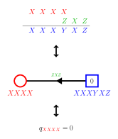
(a)

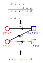
(b)

Figure 1: Graph representations of the commutators in the main text. There are subgraphs of the commutators for conserved quantities of length $4$. For blue circles, all the neighbors are drawn; for the red circles, there are some neighbors which are not critical in the argument and thus are not shown here. LABEL:sub@fig:graph_1 Graph representation of the unique possible commutator representation of the Pauli string $XXXYXZ$ in Eq. 11. LABEL:sub@fig:graph_2 The graph with the solid line is for the case of the only two possible commutator representations of the Pauli string $ZXXYXZ$ in Eq. 13. The graph with the dotted line is for a unique commutator representation of the Pauli string $YYXYZ$ in Eq. 15.

Fig. 1 shows some examples of the commutator graph for the conserved quantity of length $k$. In 1a, the commutator relation 11 is represented in a graph. Red circle represents the Pauli string $XXXX$, blue circle represents the Pauli string $XXXYXZ$, and the label above the arrow represents the Hamiltonian string $ZXZ$. Since the factor of the commutator here is $-2i$ and $r_{ZXZ}=1$, the arrow points to the red circle. In 1b, the commutator representations of 13 (solid line) and 15 (dotted line) are shown in a graph, which can be understood in a very similar way. Notice the direction of the dashed arrow, which represents the commutator relation 15. Since in the Hamiltonian we have $r_{XZ}=-1$ (see Eq.7), we need to consider the commutator relation $[\{YYXZ\}_{j},-\{XZ\}_{j+3}]=-2i\{YYXYZ\}_{j}$ to determine the weight of the edge, and thus the factor of commutator here is $-2i$ and the arrow points to the red circle.

Condition of the commutator graph. — Now we need to determine the numbers on the red circles, i.e. the coefficients of Pauli strings in conserved quantities. Recall that the numbers in red circles correspond to the coefficient of the Pauli string of $C$, $q_{{\bm{A}}^{l}}$. Then $[C,H]=0$ if and only if, for each blue circle, the sum of the numbers in the neighboring red circles multiplied by the weight of each edge must be the same with the number in the blue circle, which is zero. Thus if this condition is satisfied, then we conclude that the coefficients on the commutator graph determines the conserved quantity $C$.

This graph representation helps us to understand how the coefficients of the Pauli strings are related with each other and thus becomes zero, shown in Eqs.11-II. In Fig. 1, it becomes clear how the graph representation helps for the argument. Notice that although some circles and arrows which are not essential in our argument, are omitted, every red circle neighboring the blue circles in the graphs are all drawn. In Fig. 1a, since there is only one circle connected to the blue circle, hence $q_{XXXX}=0$. In Fig. 1b, since two circles, $ZXXX$ and $YYXZ$, are connected to the blue circle with different weight on the edge(i.e. different arrow direction on the edge), we get $q_{ZXXX}-q_{YYXZ}=0$; and since the circle $YYXZ$ is the only circle connected to the blue circle $YYXYZ$, $q_{YYXZ}=0$. Thus $q_{ZXXX}=0$.

Promising path. — In Fig. 1, we used the “path type” graphs to show the vanishing coefficient of the Pauli strings. To make the term “path type” more precisely, we define the concept called promising path. Suppose that there is a path starting from a red circle, say $A$, and ending at a blue circle, where every blue circle in the path have exactly two neighboring red circles (Note that we do not count a red circle as a neighbor when the number on it inevitably must be $0$), except the blue circle at the end which have exactly one neighboring red circle. We call this a promising path starting $A$, and if there is a promising path starting from $A$, then we call $A$ has a promising path.

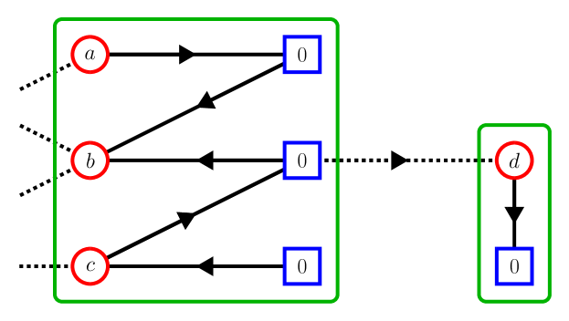
(a) Promising paths

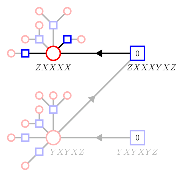
(b) Step 1

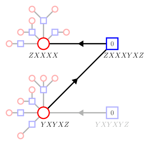
(c) Step 2-2

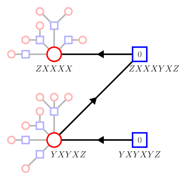
(d) Step 2-1

Figure 2: LABEL:sub@fig:ppath Promising paths. For the path in the left box, although there are three neighboring red circles in the blue circle at the middle, one of them, marked as $d$, inevitably has the number $0$ because of the promising path in the right box, this path also becomes a promising path. LABEL:sub@fig:ppath_1 Step 1 of the algorithm finding a promising path in commutator graph for the conserved quantity of length $5$. LABEL:sub@fig:ppath_2 Step 2-2 of the algorithm. LABEL:sub@fig:ppath_3 Step 2-1 of the algorithm.

Fig. 2a shows examples of promising paths starting from the red circles with $a$ and $d$ on them. Notice that, similar to the graphs in Fig.1, we can show that $d=0$, and then $a=0$ by the graph condition $a+b=0$, $b-c-d=b-c=0$, and $c=0$. In fact, no matter how long the promising path of a red circle is, the number on the red circle must be $0$. To prove it, we use induction. Let $A$ be a red circle with coefficient $q_{A}$, and the promising path of $A$ have $n$ red circles. Take $B$ as a blue circle neighboring $A$, and $C$ another red circle neighboring $B$. Then $C$ has a promising path with $n-1$ red circles, and by induction hypothesis, the coefficient of $C$, $q_{C}$, must vanish. Also, since $A$ and $C$ are the only two neighbors of $B$, $q_{A}\pm q_{C}=0$. Hence $q_{A}=0$. Since $n=1$ case can be easily shown, every red circle with promising path has vanishing coefficient. Therefore, finding a promising path directly shows the vanishing coefficient.

Finding the promising path: Algorithm. — Now we may ask how to find the promising path of a given red circle $A$. The answer uses simple inductive steps.

Step 1: scan all the neighboring blue circles, and choose the blue circles with only two or one neighbors.

Step 2-1: If a blue circle with only one neighbor is found, then we conclude that the Pauli string corresponding to a red circle $A$ is not in a conserved quantity.

Step 2-2: If we only have the blue circles with two neighbors, then choose its neighboring red circle which is not $A$ and mark it $B$.

Now repeat our process with the red circle $B$, mark new red circle which is not already chosen (i.e. neither $A$ nor $B$) as $C$(if exists), and so on. If this process terminates somehow, i.e. meets a blue circle with only one neighbor(Step 2-1), then it corresponds to a promising path. For example, Figs.2b to 2d shows how we can find the promising path of $ZXXXX$ for $k=5$ case. In Fig.2b (Step 1), when we scan all the neighboring blue circles of $ZXXXX$, then there are various neighboring blue circles, but most of them have more than three neighbors (marked with light colors) and only some of neighboring blue circles of $ZXXXX$ have exactly two neighbors(marked with dark colors). In Fig.2c (Step 2-2), we choose one among them representing the Pauli string $ZXXXYXZ$, and move onto its another neighboring red circle, $YXYXZ$. Now scan all the neighboring blue circles of $YXYXZ$ (Step 1). This gives a blue circle $YXYXYZ$ with only one neighbor, as in Fig.2d (Step 2-1), hence we found a promising path.

When the algorithm fails: Exceptions. — It turns out that in many of the Pauli strings this process terminates, and thus they have their own promising paths and thus it reduces the number of possible candidates for the conserved quantity. However, there are some red circles which do not terminates this process. We can classify them into two categories.

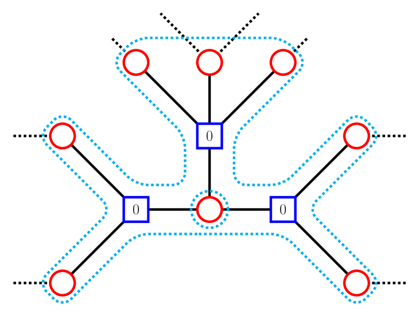
(a) Exception 1

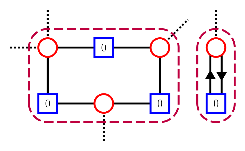
(b) Exception 2

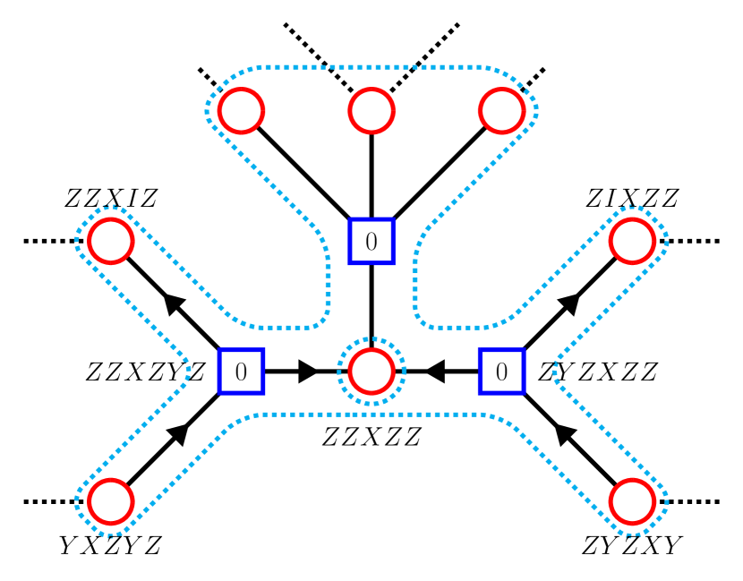
(c) Exception 1: example

(d) Exception 2: example

Figure 3: LABEL:sub@fig:exception_1 First exception when we cannot find a promising path. Every blue neighboring circles of the red circle in the center of the figure has $\geq 3$ neighboring red circles, and thus we are not sure the red circle in the center has a promising path. LABEL:sub@fig:exception_2 Second exception when we cannot find a promising path. Although every blue circles have $\leq 2$ neighboring red circles, we cannot find a blue circle with $1$ neighboring red circle, and thus we get an endless loop. LABEL:sub@fig:exception_1_exmp An example of Exception 1 for $k=4$. LABEL:sub@fig:exception_2_exmp An example of Exception 2 for $k=4$.

Exception 1. Fig. 3a shows the case when we cannot find the neighboring blue circles with only one or two neighbors, since every neighboring blue circles have more than two neighbors; i.e., violating Step 1. In this case we cannot convince that the number on the red circle must be $0$. Exception 1 case occurs frequently when we try to consider the commutator representation of the Pauli string with length $\leq k$, since in this case there would be various commutator representations where the Hamiltonian string places on the middle. Since for the Pauli strings with length $>k$ the position of the Hamiltonian string in the commutator representation is on the edge of the Pauli string, focusing on the length $>k$ blue circled Pauli strings is a good strategy to avoid the Exception 1 cases. Indeed there are some Hamiltonians, including $XYZ+h$ modelShiraishi (2019), which do not contain Exception 1 cases when we focus on length $k+1$ blue circled Pauli strings. However there are some models, including PXP models, which contains Exception 1 errors even when we focus on length $>k$ blue circled Pauli strings. For example, Fig. 3c shows that the Pauli string $ZZXZZ$ belongs to Exception 1 for $k=5$ in PXP model, even if we scan all the length $6$ blue circled Pauli strings such as $ZZXZYZ$ or $ZYZXZZ$. However, we show that in the PXP model these kinds of Exception 1 red circles actually always have a promising path. More precisely, if we remove every red circle having a promising path, then we can see that at least one neighboring blue circle have only one or two neighbors, hence we can still use Step 1.

Exception 2. In Fig 3b, alternating red and blue circles form a closed loop, thus, the loop never ends, i.e. in Step 2-2 we meet a red circle that has already passed through. In this case, we cannot determine the number on the red circle to be $0$. For example, Fig. 3d shows that the Pauli string $ZXYYZ$ is in Exception 2 for $k=5$. This is a bit tricky case since, unlike Exception 1, this Exception 2 case occurs in every system, and for integrable systems this kind of loops actually correspond to the conserved quantities. We show that in the PXP model, every conserved quantity with this endless loop-type graph representations are trivial.

Thus, if the coefficients of the Pauli strings in these two exceptional “error” cases are shown to be zero, then it is enough to conclude that there are no nontrivial local conserved quantities in the system. Our natural question is whether a certain Pauli string has a promising path or belongs to Exception 1 or 2. In the following section, we suggest the way which makes possible to categorize the Pauli strings, which is a very simple and systematic and thus can possibly be generalized into any other Hamiltonians.

Before going further, here we emphasize that this categorization holds for every spin-$1/2$ system. For example, in [21] we can see that every Pauli string which are not “doubling-product operator” have zero coefficients. The Pauli strings that are not “doubling-product operator” correspond to the Pauli strings with promising path, and the “doubling-product operators” correspond to the Exception 2. In this case we do not have any operators corresponding to Exception 1 as mentioned before, which makes the proof a bit easier. Other various spin-$1/2$ models will be treated in Appendix F.

IV Categorizing the Pauli strings: PXP model

Pauli String Type	Initial and Final Operators (Length $k$)			Resolved by Theorem…
Simple cases	$\begin{bmatrix}X\\ Y\end{bmatrix}$	$\cdots$	$\begin{bmatrix}X\\ Y\end{bmatrix}$	1*
	$Z\begin{bmatrix}Y\\ Z\\ I\end{bmatrix}$	$\cdots$	$\begin{bmatrix}X\\ Y\end{bmatrix}$	2
	$ZX$	$\cdots$	$\begin{bmatrix}X\\ Y\end{bmatrix}$	3
Exception 1: Category 1	$Z\begin{bmatrix}Z\\ I\end{bmatrix}$	$\cdots$	$\begin{bmatrix}Z\\ I\end{bmatrix}Z$	8
Exception 1: Category 2	$ZY\begin{bmatrix}Z\\ I\end{bmatrix}$	$\cdots$	$\begin{bmatrix}X\\ Y\end{bmatrix}Z$	5*
Exception 1,2: Category 3	$ZX\begin{bmatrix}X\\ Y\end{bmatrix}$	$\cdots$	$\begin{bmatrix}X\\ Y\end{bmatrix}Z$	4, 5*, 6 and 7
Exception 2	$ZY\begin{bmatrix}X\\ Y\end{bmatrix}$	$\cdots$	$\begin{bmatrix}X\\ Y\end{bmatrix}Z$	5*, 6 and 7
Others	$ZX\begin{bmatrix}Z\\ I\end{bmatrix}$	$\cdots$	$\begin{bmatrix}X\\ Y\end{bmatrix}Z$	5*
	$Z\begin{bmatrix}Z\\ I\end{bmatrix}$	$\cdots$	$\begin{bmatrix}X\\ Y\end{bmatrix}Z$

Table 1: Pauli string types, their initial and final Pauli operator sequences, and how they resolved(i.e. shown to have a vanishing coefficient or gives trivial conserved quantity). If a Pauli string is included in a single Pauli string type, then its reflected one is also included in such a single Pauli string type. The Pauli operators written vertically represents the possible choices in the initial or final Pauli operator sequence. Theorem number with asterisk * means that the proof is in the main text; the others have their proofs in appendix.

Outline. — In this section, we categorize the length $k$ Pauli strings for the PXP model. As argued above, there are only three possibilities for a single Pauli string: it has a promising path, or is belonged to Exception 1 or 2. The Pauli strings which do not start or end with $Z$ can be simply shown that they have a promising path: the list of them are given in the following Theorem 1, 2, and 3(See “Simple cases” in Table 1). So all we need to do is carefully search for the Pauli strings that begin and end with $Z$. All the other Pauli strings (except some cases, which can also simply be shown to have a promising path, but are treated together with others for brevity: See “Others” in Table 1), are included in Exception 1 or Exception 2 cases; some in both(i.e. every neighboring blue circle has more than two neighbors and we always find the endless loop). We argue that the cases in Exception 1 occurs due to the “unexpected” commutator representation, which will be explained later, and we classify them into three categories according to the position of the Hamiltonian string for these unexpected commutator represetations: Category 1, 2, and 3.

From the definition, there is neighboring blue circles of the red circle in Category 1 and 2 only have less than or equal to $4$ neighboring red circles, while in Category 3 every neighboring blue circles have many neighboring red circles, proportional to the system size. Theorem 4 first shows that we can ignore most of the neighbors of Category 3 except two. This greatly reduces the possibility of scanning the promising path, and leads us to Theorem 5, showing that every Pauli strings in Category 2 have a promising path (See “Exception 1: Category 2” in 1), and every Pauli strings in Category 3 can be considered as Exception 2 case: i.e. we always find the endless loop. Focusing on Exception 2, we show that every Pauli strings in Exception 2 are (exclusively) included in one of two loops. In Theorem 6 and Theorem 7, we show that one of the Pauli string in each loop, hence every Pauli string in each loop, has a vanishing coefficient. (See “Exception 1,2: Category 3” and “Exception 2” in Table 1). Finally, Theorem 8 shows that if a conserved quantity $C$ contains one of the Pauli strings in Category 1, then $C$ is trivial (See “Exception 1: Category 1” in 1). This concludes our main result.

Simple cases. — We start with the simple case, which does not start and end with $Z$.

Theorem 1. In the commutator graph for the conserved quantity of length $k$, each Pauli string with length $k$ that does not start and end with $Z$ have a promising path.

Proof. Let $A_{1}A_{2}\cdots A_{k}$ be a Pauli string where $A_{1},A_{k}\neq Z$. Now consider the following commutator relation.

$$\begin{array}[]{rrrrrrr}&A_{1}&A_{2}&\cdots&A_{k}&&\\ &&&&Z&X&Z\\ \hline\cr&A_{1}&A_{2}&\cdots&\overline{A_{k}}&X&Z\end{array}$$ (17)

Here, $\overline{A_{k}}=Y$ if $A_{k}=X$, and $\overline{A_{k}}=X$ if $A_{k}=Y$. This shows the red circled Pauli string $A_{1}A_{2}\cdots A_{k}$ is connected to the blue circled Pauli string $A_{1}A_{2}\cdots\overline{A_{k}}XZ$. If there is another red circled Pauli string connected to the blue circled Pauli string, then the only possible form is the following:

$$\begin{array}[]{rrrrrrrr}&A_{1}&A_{2}&A_{3}&\cdots&A_{k}&X&Z\\ &Z&X&Z&&&&\\ \hline\cr&B_{1}&?&?&\cdots&\overline{A_{k}}&X&Z\end{array}$$ (18)

This is because the blue circled Pauli string has length $k+2$, and because every connected red circled Pauli string must be written by the commutator between the blue circled Pauli string and a Hamiltonian string. But if we use any other Hamiltonian string or put $ZXZ$ on any other position, then the resulting commutator has length $\geq k+1$, thus they cannot be length $\leq k$ red circled Pauli string. But since $A_{1}\neq Z$, $B_{1}\neq I$ and thus even the commutator in Equation 18 gives length $k+2$ Pauli string. Thus there is no other neighbor to the blue circled Pauli string, and gives the promising path for $A_{1}A_{2}\cdots A_{k}$. $\square$

Recall that, for $k=4$, Equation 11 is a perfect example for this Theorem.

The proof of this theorem can be easily extended into the Pauli strings starting with $ZY,ZZ,$ or $ZI$ and not ending with $Z$, or their reflected forms (i.e. Pauli strings ending with $ZY,ZZ,$ or $ZI$ and not starting with $Z$).

Theorem 2. In the commutator graph for a conserved quantity of length $k$, any Pauli string with length $k$ starting with $ZY,ZZ,$ or $ZI$ and not ending with $Z$, or their reflected forms, have a promising path.

Proof. See Appendix B.

For the Pauli strings starting with $ZX$ and not ending with $Z$ (and their reflected forms), our proof does not work; a nice example is Equation 13. The cause of the failure is because there are possibly two red circled Pauli strings (in the example, $ZXXX$ and $YYXZ$) to a given blue circled Pauli string (in the example, $ZXXYXZ$). However, we can still easily find a promising path, using slightly different strategy. Since the basic idea is very similar with above theorems, we omit the proof of the following Theorem and describe it in Appendix B.

Theorem 3. In the commutator graph for a conserved quantity of length $k$, any Pauli string with length $k$ starting with $ZX$ and not ending with $Z$, or their reflected forms, have a promising path.

Proof. See Appendix B.

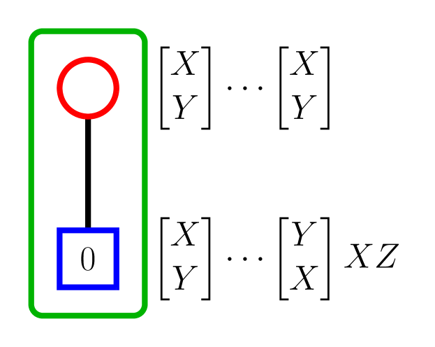
(a) Theorem 1: Proof.

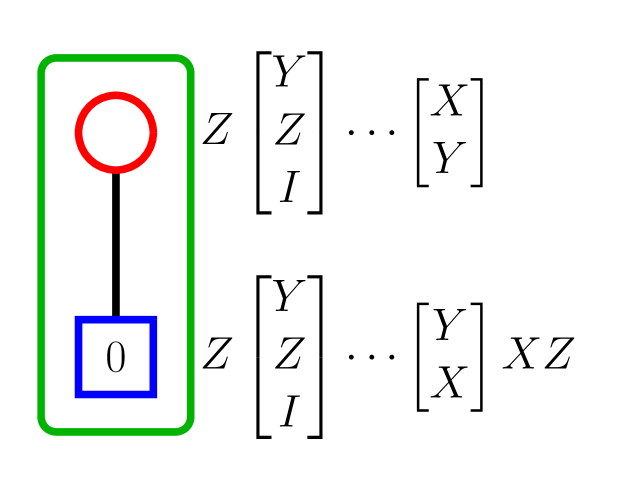
(b) Theorem 2: Proof.

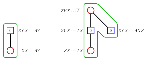
(c) Theorem 3: Proof.

Figure 4: The proofs of LABEL:sub@fig:thm_1 Theorem 1, LABEL:sub@fig:thm_2 Theorem 2, and LABEL:sub@fig:thm_3 Theorem 3. The green boxes represent Promising paths.

Theorem 1, 2, and 3 shows that every Pauli string with length $k$ which do not start or end with $Z$ has a promising path. This result not only reduces the number of Pauli string candidates related to a conserved quantity, if any, but also plays an important role in the proof of the future Theorems. Notice that the proofs of Theorem 1, 2, and 3 can be simply represented in the form of graph, as we can see in Fig. 4.

Importance of edge. — Through the proof of Theorem 1, 2, and 3, we can observe the similarity between them. We take the commutator between red circled Pauli string and Hamiltonian string, positioning Hamiltonian string on the “edge”, i.e. left or right edge of the Pauli string. Because this process always gives the blue circled Pauli string with length $>k$, the only possible choice is again taking the commutator between blue circled Pauli string and Hamiltonian string, positioning Hamiltonian string on the edge. Hence the number of candidate of the red circled Pauli strings neighboring the blue circled Pauli string is very small, making us easier to find a promising path. Indeed, in the proof of Theorem 1, 2, and 3, this method gives at most two neighboring red circled Pauli strings, which directly fits in the process of finding a promising path. Like this, if the two possible commutator representation of the blue circled Pauli string comes from the commutator positioning Hamiltonian string one on the left and the other on the right, then we call them “expected” commutator representations.

For example, suppose that we are finding a promising path starting from the Pauli string $ZZYXZ$ for $k=5$. The simplest approach we can do is to commute $XZ$ operator on the right edge, giving the Pauli string $ZZYXYZ$. Since we have already considered the commutator on the right, another “expected” commutator representations of this Pauli string should be on the left side: indeed, we have the following relation.

$$\begin{array}[]{rrrrrrr|l}&Z&Z&Y&X&Z&&\textrm{Baseline}\\ &&&&&X&Z&\\ \hline\cr&Z&Z&Y&X&Y&Z&\\ \hline\cr&&Y&Y&X&Y&Z&\textrm{Expected}\\ &Z&X&&&&&\textrm{representation}\\ \end{array}$$ (19)

This is the possible candidate of the route of a promising path of the Pauli string $ZZYXZ$: indeed, since the Pauli string $YYXYZ$ has a promising path as we have already shown in Theorem 2, we can show that the Pauli string $ZZYXZ$ also has a promising path.

Putting and pulling method. — Eq.19 can be considered as “putting” $XZ$ operator on the right(baseline) and “pulling” $ZX$ operator from the left of the Pauli string(expected representation). Because this is the basic strategy finding the promising path of given Pauli string, we need to define it precisely as following. “Putting” the Hamiltonian string on the right edge of the Pauli string means taking the commutator between Hamiltonian string and the Pauli string where the Hamiltonian string positions on the right edge and getting the Pauli string longer than the original one, as we can see in the “Baseline” commutator relation in Eq.19. “pulling” the Hamiltonian strong from the left edge of the Pauli string means writing down the commutator representation between Hamiltonian string and the Pauli string where the Hamiltonian string positions on the left edge, as we can see in the “Expected representation” commutator rperesentation in Eq. 19. One may expect that this putting and pulling method gives at most two commutator representations, hence for a given Pauli string, we can try to find out a promising path of it by putting and pulling Hamiltonian strings repeatitively.

“Unexpected” commutator representations. — However, when we investigate the Pauli strings starting and ending with $Z$ operators, we sometimes get “unexpected” commutator representations on the edge, which is not expected on the putting and pulling method and hence gives more than two neighboring red circled Pauli string to the blue circled Pauli strings, classified as the Exception 1 cases. Since this “unexpected” commutator representation occurs on the various positions of the Pauli string, and because, depending on the position of the “unexpected” commutator, the way to resolve those exceptional cases differs, it is convenient to classify the Exception 1 cases into a smaller category. We can divide them into three categories, distinguished by the position of the Hamiltonian string for the “unexpected” commutator representations: right, left, or middle. Notice that this classification is general, and can be applied to general cases of the spin-$1/2$ Hamiltonian.

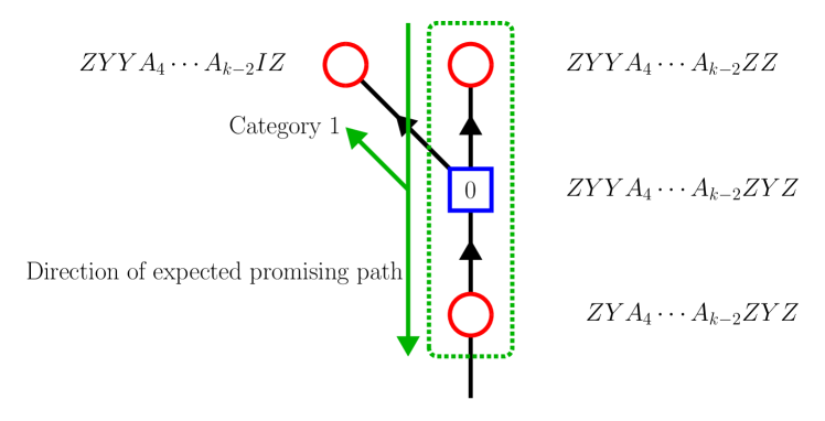
(a) Exception 1: Category 1.

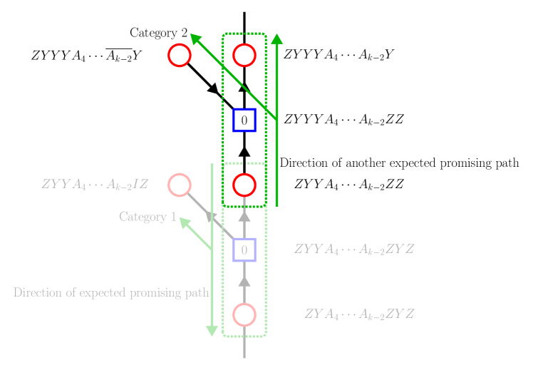
(b) Avoiding Category 1.

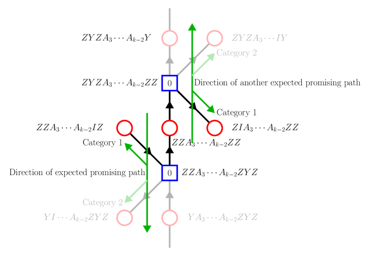
(c) Impossible to avoid Category 1.

Figure 5: LABEL:sub@fig:thm_1 The diagrammatic representation of Category 1. LABEL:sub@fig:thm_2 The case when we can avoid Category 1 case. LABEL:sub@fig:thm_3 The case when we cannot avoid Category 1 case. Green boxes represent the expected Pauli strings, and green arrows represent their directions.

Category 1. Consider the red circled Pauli string starting with $ZYY$ and ending with $ZZ$. Take the commutator with Hamiltonian string $XZ$ on the right edge, and get the blue circled Pauli string with length $k+1$. In this case, except the “expected” commutator representation on the left edge, there is another commutator representation on the right edge. Indeed, we can see that

$$\begin{array}[]{rrrrrrrrrrr|l}&Z&Y&Y&A_{4}&\cdots&&A_{k-2}&Z&Z&&\textrm{Baseline}\\ &&&&&&&&&X&Z&\\ \hline\cr&Z&Y&Y&A_{4}&\cdots&&A_{k-2}&Z&Y&Z&\\ \hline\cr&{\color[rgb]{1,0,0}Z}&{\color[rgb]{1,0,0}Y}&{\color[rgb]{1,0,0}Y}&{\color[rgb]{1,0,0}A_{4}}&{\color[rgb]{1,0,0}\cdots}&&{\color[rgb]{1,0,0}A_{k-2}}&{\color[rgb]{1,0,0}I}&{\color[rgb]{1,0,0}Z}&&\textrm{Cat 1}\\ &&&&&&&&{\color[rgb]{1,0,0}Z}&{\color[rgb]{1,0,0}X}&{\color[rgb]{1,0,0}Z}&\\ \hline\cr&&Z&Y&A_{4}&\cdots&&A_{k-2}&Z&Y&Z&\textrm{Expected}\\ &Z&X&&&&&&&&&\textrm{representation}\\ \end{array}$$ (20)

which gives three neighboring red circled Pauli strings. Here, a red-colored second commutator representation is an unexpected commutator representation with Hamiltonian string on the right. See Fig.5a for the diagrammatic explanation. In the graph description, we can see that while we are following the expected promising path by putting Hamiltonian string on the right of the Pauli string and pulling Hamiltonian string from the left of the Pauli string, the promising path “bounce back” by unexpected commutator representation on the right edge. Similar thing happens to the Pauli string ending with $IZ$.

If the Pauli string does not start with $ZZ$ or $ZI$ but start with $ZX$ or $ZY$, then we can avoid Category 1 case, by taking the different direction of expected promising path: i.e. putting Hamiltonian string $ZX$ on the left edge and pulling Hamiltonian string from the right of the Pauli string. See Fig.5b for details. In this case, although there is a different type of unexpected representation (which is called Category 2 case and will be treated later), but we do not need to consider the Category 1 case now. On the other hand, if the Pauli string ends with $ZZ$ or $IZ$ and starts with $ZZ$ or $ZI$, it is impossible to neglect the Category 1 but one should consider it. In Fig.5c, we can see that in both direction of expected promising path, the Category 1 case appear. Indeed, the Pauli strings in this category are strongly related to the trivial operators defined in Theorem 1. We will come back to analyze these Pauli strings, starting with $ZZ$ or $ZI$ and ending with $ZZ$ or $IZ$ and now we focus on other cases, i.e., the Pauli strings which start or end with $XZ$ or $YZ$. In this case it is enough to treat the Pauli strings which do not end with $ZZ$ or $IZ$: For the Pauli strings which end with $ZZ$ or $IZ$ and start with $ZX$ or $ZY$, the logics are same with the Pauli strings which start with $ZZ$ or $ZI$ and end with $XZ$ or $YZ$, due to the mirror symmetry of the Hamiltonian.

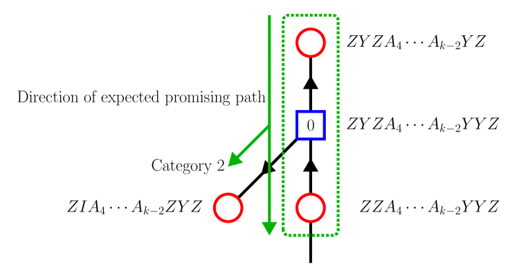
Figure 6: The diagrammatic representation of Category 2.

Category 2. Consider the red circled Pauli string starting with $ZYZ$ and ending with $Z$. Take the commutator with Hamiltonian string $XZ$ on the right edge, and get the blue circled Pauli string with length $k+1$. In this case, except the “expected” commutator representation on the left edge, there is another commutator representation on the left edge. Indeed, we can see that

$$\begin{array}[]{rrrrrrrrrrr|l}&Z&Y&Z&A_{4}&\cdots&&A_{k-2}&Y&Z&&\textrm{Baseline}\\ &&&&&&&&&X&Z&\\ \hline\cr&Z&Y&Z&A_{4}&\cdots&&A_{k-2}&Y&Y&Z&\\ \hline\cr&&Z&Z&A_{4}&\cdots&&A_{k-2}&Y&Y&Z&\textrm{Expected}\\ &Z&X&&&&&&&&&\textrm{representation}\\ \hline\cr&&{\color[rgb]{1,0,0}Z}&{\color[rgb]{1,0,0}I}&{\color[rgb]{1,0,0}A_{4}}&{\color[rgb]{1,0,0}\cdots}&&{\color[rgb]{1,0,0}A_{k-2}}&{\color[rgb]{1,0,0}Y}&{\color[rgb]{1,0,0}Y}&{\color[rgb]{1,0,0}Z}&\textrm{Cat 2}\\ &{\color[rgb]{1,0,0}Z}&{\color[rgb]{1,0,0}X}&{\color[rgb]{1,0,0}Z}&&&&&&&&\\ \end{array}$$ (21)

which gives three neighboring red circled Pauli strings. Here, a red-colored third commutator representation is an unexpected commutator representation with Hamiltonian string on the left. See Fig.6 for the diagrammatic explanation. In the graph description, we can see that while we are following the expected promising path by putting Hamiltonian string on the right of the Pauli string and pulling Hamiltonian string from the left of the Pauli string, the promising path is “branched” by unexpected commutator representation on the left edge. Similar thing happens to the Pauli string starting with $ZYI,ZZZ,$ or $ZZI$ (or their reflected forms).

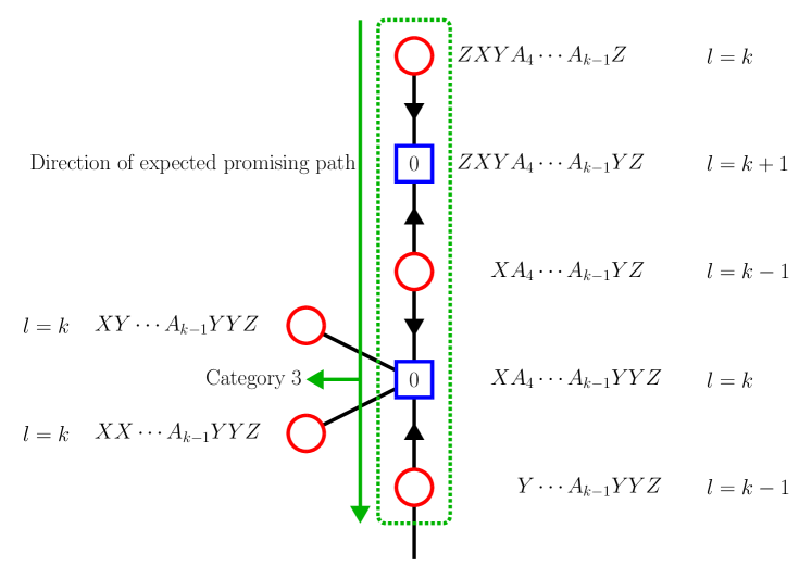
Figure 7: The diagrammatic representation of Category 3.

Category 3. Consider the Pauli string starting with $ZXY$ and ending with $Z$. Take the commutator with Hamiltonian string $XZ$ on the right edge, and get the blue circled Pauli string with length $k+1$. This Pauli string have another neighboring red circled Pauli string, which has length $k-1$, as we can see below.

$$\begin{array}[]{rrrrrrrrrrr|l}&Z&X&Y&A_{4}&\cdots&&A_{k-1}&Z&&&l=k\\ &&&&&&&&X&Z&&\\ \hline\cr&Z&X&Y&A_{4}&\cdots&&A_{k-1}&Y&Z&&l=k+1\\ \hline\cr&&&X&A_{4}&\cdots&&A_{k-1}&Y&Z&&l=k-1\\ &Z&X&Z&&&&&&&&\\ \end{array}$$ (22)

In this case there are only two commutator representation, and we have no unexpected commutator representation. The problem occurs when we try to do the same job on the length $k-1$ Pauli string. In this case, there are possibly a lot of neighboring red circled Pauli strings. For example,

$$\begin{array}[]{rrrrrrrrrrrr|l}&X&Y&A_{3}&A_{4}&\cdots&&A_{k-2}&Y&Z&&&l=k-1\\ &&&&&&&&&X&Z&&\textrm{Baseline}\\ \hline\cr&X&Y&A_{3}&A_{4}&\cdots&&A_{k-2}&Y&Y&Z&&l=k\\ \hline\cr&&X&?&?&\cdots&&A_{k-2}&Y&Y&Z&&l=k-1\\ &X&Z&&&&&&&&&&\textrm{Exp. rep.}\\ \hline\cr&{\color[rgb]{1,0,0}X}&{\color[rgb]{1,0,0}Y}&{\color[rgb]{1,0,0}?}&{\color[rgb]{1,0,0}?}&{\color[rgb]{1,0,0}\cdots}&&{\color[rgb]{1,0,0}A_{k-2}}&{\color[rgb]{1,0,0}Y}&{\color[rgb]{1,0,0}Y}&{\color[rgb]{1,0,0}Z}&&l=k\\ &&&{\color[rgb]{1,0,0}Z}&{\color[rgb]{1,0,0}X}&&&&&&&&\textrm{Cat 3}\\ \hline\cr&{\color[rgb]{1,0,0}X}&{\color[rgb]{1,0,0}X}&{\color[rgb]{1,0,0}?}&{\color[rgb]{1,0,0}?}&{\color[rgb]{1,0,0}\cdots}&&{\color[rgb]{1,0,0}A_{k-2}}&{\color[rgb]{1,0,0}Y}&{\color[rgb]{1,0,0}Y}&{\color[rgb]{1,0,0}Z}&&l=k\\ &&{\color[rgb]{1,0,0}Z}&{\color[rgb]{1,0,0}X}&{\color[rgb]{1,0,0}Z}&&&&&&&&\textrm{Cat 3}\\ \hline\cr&&&&&\vdots&&&&&&&\\ \end{array}$$ (23)

Here, a red-colored third and fourth commutator representations (and many other possible representations that are not shown here) are unexpected commutator representations with Hamiltonian string in the middle. This happens because the length of blue circled Pauli string is $k$, hence for the commutator, the position of Hamiltonian string is not needed to be on the edge. See Figure 7 for the diagrammatic explanation. In the graph description, we can see that while we are following the expected promising path by putting Hamiltonian string on the right of the Pauli string and pulling Hamiltonian string from the left of the Pauli string, the promising path is “dissipated” by various edges connected to the blue circle. Similar thing happens to the Pauli string starting with $ZXX$.

Summary in Exception 1. — In summary, when we take the commutator with Hamiltonian string $XZ$ on the right edge, Type 1 Exception occurs when the unexpected other commutator representations are present with Hamiltonian strings on the (i) right edge of a Pauli string for Category 1, (ii) left edge for Category 2, and (iii) middle for Category 3. Of course we may put the Hamiltonian string $ZX$ on the left edge, but categorizing this case can be simply done by mirror reflecting Category 1, 2, and 3 above. As a result, we fully categorized the Pauli strings which generates Type 1 exception.

Treating Category 3. — Now we show that the exceptions in Category 3 can be well treated. Because there are too many neighboring red circles in Category 3, treating them first make our problem more simple. Indeed, we can show that all the Category 3 cases can be reduced into Category 2 cases. The proof is based on Theorem 1 to 3, which removed a number of Pauli strings with vanishing coefficient, which is a core in the proof of the following Theorem.

Theorem 4. In the commutator graph of the PXP model with the conserved quantity of length $k$, consider a red circled Pauli string with length $k-1$ ending with $Z$ and not starting with $Z$, or their reflected forms. Then we can always find its neighboring blue circled Pauli string, by putting the Hamiltonian string on the right side of the Pauli string, where all the numbers in its neighboring red circles are $0$ except at most three red circles: the two expected representations, and the Category 2 type unexpected representation.

Proof. See Appendix B.

We can summarize the proof of Theorem 4 as following: It is unnecessary to consider the commutator representation with the Hamiltonian string in the middle of the Pauli string. We only need to consider when the Hamiltonian string is placed on the edges. Furthermore, if we ignore the operators $ZZ\cdots ZZ$, $ZI\cdots ZZ$, $ZZ\cdots IZ$, or $ZI\cdots IZ$ then we can always avoid the Category 1 cases by the argument described in Fig.5b, and only need to treat Category 2 cases.

Treating Category 2. — Now we analyze the Category 2 case. In Fig.6, In the direction of the expected promising path, it has “branches”. On each branch, we can still put $XZ$ operator on the right and pull the Hamiltonian operator from the left. This is possible since (i) we have already figured out that every Category 3 case can be removed and it is considered as Category 2 cases, and (ii) putting $XZ$ operator on the right never creates the Category 1 case, since the right edge will always become $\cdots YZ$. Therefore the only case we need to worry is the Exception 2 case: the loop case.

Now we return to Equation 21 with the graph representation Fig.6 . Here, we can see that the red circled Pauli string starting with $ZYZ$ and ending with $Z$ is neighboring to the blue circled Pauli string, whose other red circled neighbors are the Pauli string starting with $ZZ$ or $ZI$, and ending with $Z$. As we have argued before, because they always end with $YZ$, they never fall into the Category 1. Choose one Pauli string, say, the one starting with $ZZ$. By putting Hamiltonian string $XZ$ on the right edge, get the blue circled Pauli string with length $k+1$, and searching its red circled neighbors, we get the following.

$$\begin{array}[]{rrrrrrrrrr}&Z&Z&A_{4}&\cdots&&A_{k-1}&Y&Z&\\ &&&&&&&&X&Z\\ \hline\cr&Z&Z&A_{4}&\cdots&&A_{k-1}&Y&Y&Z\\ \hline\cr&&Y&A_{4}&\cdots&&A_{k-1}&Y&Y&Z\\ &Z&X&&&&&&&\\ \hline\cr&&Y&\overline{A_{4}}&\cdots&&A_{k-1}&Y&Y&Z\\ &Z&X&Z&&&&&&\\ \hline\cr\end{array}$$ (24)

Here $\overline{A_{4}}=I,Z$ if $A_{4}=Z,I$ respectively; otherwise the last commutator representation vanishes. This shows that, for the red circled Pauli string starting with $ZZ$ and ending with $Z$, we can find a neighboring blue circled Pauli string, whose other red circled neighbors start with $Y$ and end with $Z$ and with length $k$: again Category 2 case. But we have already shown in Theorem 2 and 3 that the numbers in these red circles must be zero. Hence the only possibly nonzero red circled neighbor of the blue circle is $ZZA_{4}\cdots A_{k-1}YZ$ itself, guaranteeing a promising path. Similarly, we can show that the red circled Pauli string starting with $ZI$ and ending with $Z$ has a neighboring blue circled Pauli string, whose other red circled neighbors start with $X$ and end with $Z$ and with length $k$: Category 2 case. Again the numbers in these red circles must be zero, hence we get the promising path to the Pauli string starting with $ZI$ and ending with $Z$. These facts then, again, directly show that the Pauli string starting with $ZYZ$ and ending with $Z$ has a promising path.

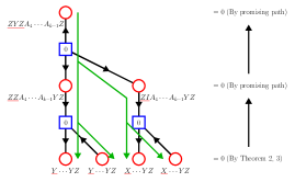
(a)

(b)

Figure 8: (a) Graph representation showing the coefficient of $ZYZA_{4}\cdots A_{k-1}Z$ vanishes. The thick arrow shows the logical direction we follow. (b) Flowchart of the left edge Pauli substring. Each box represents the set of Pauli strings whose left edge substring is the Pauli string inside the box. Following the arrow, we can see that how the left edge Pauli substring changes as we keep put $XZ$ operator on the right and pull Hamiltonian string from the left.

Figure 8(a) shows how we showed that the Pauli string starting with $ZYZ$ and ending with $Z$ has a promising path. Notice that, because we are only considering Category 2 case, for each step the details in the middle and right edge of the Pauli string are not very important, and only the left edge Pauli substrings are important. Figure 8(b) is a simplified figure, only with the information of the left edge Pauli substring. We start with the length $k$ $ZYZ-$ Pauli string, then goes into the length $k$ $ZZ-$ and $ZI-$ Pauli strings, then length $k$ $X-$ and $Y-$ Pauli strings, and we stop here, concluding all their coefficients are zero based on Theorem 2 and 3. We can do this job for every other possible left edge substring of the Pauli strings.

As we have done above, one can determine if the Pauli string has a promising path or not, only by tracking the left edge. We can formalize this statement into Theorem 5, which finally characterizes every Pauli strings with or without a promising path.

Theorem 5. For the Pauli string not starting with $ZZ$ or $ZI$ and not ending with $IZ$ or $ZZ$, the followings hold:

1. If the Pauli string starts and ends with $Z$, and between these $Z$’s there are only $X$ or $Y$ operators, then it is in Type 2 Exception. More precisely, every such operator with even number of $X$ operators constructs a loop, and every such operators with odd number of $X$ operators constructs another loop.

2. If not, then the Pauli string has a promising path.

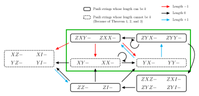
Figure 9: Flowchart of the leftmost sequences of the Pauli string. See the Proof of Theorem 5 for details.

Proof. As we have done before, we can draw the flowchart for every possible left edge Pauli substring of the Pauli strings, see Figure 9. We read the figure as following. Consider a red circled Pauli string $P$. Find the box including the left edge Pauli substring of $P$ in the Figure, then track the arrow, and collect all the leftmost sequences in the boxes at the end of the arrow. If the color of the arrow is red (blue) then the length of the red colored Pauli string increases (decreases) by $1$ compared to $P$. Here are some examples. (i) If $P$ is a length $k$ Pauli string starting with $ZXZ-$, then we can find its neighboring blue circle whose other neighbors are represented by length $k$ Pauli strings starting with $ZZ-$ or $ZI-$ (ii) If $P$ is a length $k-1$ Pauli string starting with $YX-$, then we can find its neighboring blue circle whose other neighbors are represented by length $k$ Pauli strings starting with $ZXY-,ZXX-,ZYX-,$ or $ZYY-$, and so on. Notice that the number of neighbors are not restricted; there can be no such neighbors, or there can be more than one such neighbors.

From the definition of the flowchart, we can see the following: If we start from a particular box and follow the arrows, and always reach the boxes including the left edge Pauli substrings starting with $X-$ or $Y-$(the dashed boxes) with length $k$, then since those Pauli strings have promising paths and hence have vanishing coefficients, each Pauli string whose left edge Pauli substring is included in the initial box has a promising path, by similar logic in Fig.8.

Now we scan each possibilities.

Suppose that we have a length $k$ Pauli string starting with $ZZ-$ or $ZI-$. Following the arrows, we get length $k$ Pauli strings starting with $X-$, $Y-$. Hence each Pauli string starting with $ZZ-$ and $ZI-$ has a promising path.

Suppose that we have a length $k$ Pauli string starting with $ZXZ-$, $ZXI-$, $ZYZ-$, or $ZYI-$. Following the arrow, we get length $k$ Pauli strings starting with $ZZ-$, $ZI-$. Then, again following the arrows, we get length $k$ Pauli strings starting with $X-$, $Y-$. Hence each Pauli string starting with $ZXZ-$, $ZXI-$, $ZYZ-$, or $ZYI-$ also has a promising path.

Now we consider a length $k$ Pauli string starting with $ZYX-$ or $ZYY-$. Suppose that (possibly after some self-loop) we follow the arrow toward the box containing $ZXZ-$ and others. In this case, by the same logic above, we can conclude that the Pauli string have a promising path. This always happens when there is $Z$ or $I$ operator between two $Z$ left and right edge operators.

Similarly, consider a length $k$ Pauli string starting with $ZXY-$ or $ZXX-$. Suppose that we follow the arrow toward the box containing $XZ-$ and others, with length $k-1$. In this case, by following arrow again we get length $k$ Pauli strings starting with $ZZ-$, $ZI-$, then by the same logic above, we can conclude that the Pauli string have a promising path. This always happens when there is $Z$ or $I$ operator between two $Z$ left and right edge operators. Suppose, now, that we follow the arrow toward the box containing $XY-$ and $XX-$, then (possibly after some self-loop) toward the box containing $XZ-$ and so on. Again, by the same logic, one can conclude that the Pauli string have a promising path, and this happens when there is no $Z$ or $I$ character between two $Z$ leftmost and rightmost operators.

In summary, If we leave the area drawn by the green box, then our process always terminates and gives a promising path; it does not happens if there are only $X$ or $Y$ operators between two $Z$ operators of the length $k$ Pauli string, showing the statement 2. For the detailed study of the cases in the green box, we draw another flowchart, which describes the flows in the green box with more details.

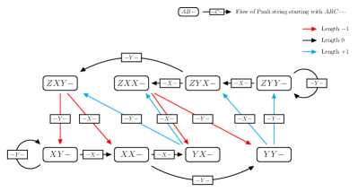
Figure 10: Detailed flowchart inside the green box of Figure 9. The symbols on the arrows represents the Pauli matrices right next to the Pauli substrings on the tail of the arrow. See the Proof of Theorem 5 for more details.

In Figure 10, we draw the flowchart for every possible initial sequences in the green box in Figure 9. Here, we ignored the arrows toward or from the outside of the green box, since we already know that such flow always terminate. The characters on the arrow represents the operator which is placed just right to the left edge substring. For example, if we want to track the change of the left edge substring of the Pauli string starting with $ZXXY\cdots$, when we choose a red arrow starting from $ZXX-$ with symbol $-Y-$ on it. Because taking the commutator with $XZ$ operator on the right side of the Pauli string ending with $Z$ always produces the Pauli string ending with $YZ$, e.g.

$$\begin{array}[]{rrrrrrr}&Z&A_{2}&\cdots&A_{k-1}&Z&\\ &&&&&X&Z\\ \hline\cr&Z&A_{2}&\cdots&A_{k-1}&Y&Z\\ \end{array}$$ (25)

we can conclude that every Pauli string with length $k$ which can endlessly follow the flow of Figure 10 starts and ends with $Z$, and between these $Z$’s there are only $X$ and $Y$ operators. Furthermore, because each step in Figure 10 do not decrease the number of $Y$ operators, the flow always terminates on the endless loop of either $\underbrace{ZYY\cdots YYZ}_{k}$ or $\underbrace{XY\cdots YYZ}_{k-1}$, which gives a Type 2 Exception. Finally, beacuse each step in Figure 10 also does not change the number of $X$ operators modular $2$, every Pauli strings in statement 1 are included in either the loop of $\underbrace{ZYY\cdots YYZ}_{k}$ or $\underbrace{XY\cdots YYZ}_{k-1}$, which shows the statement 1. $\square$

By Theorem 1 $-$ 5, we show that all the Pauli string with length $k$ has a vanishing coefficient, except:

1. Pauli string $\underbrace{ZYY\cdots YYZ}_{k}$, or the other Pauli strings with length $k$ starts and ends with $Z$, and between these $Z$’s there are only $X$ or $Y$ operators, where the number of $X$ operators is even;

2. The Pauli string $\underbrace{XY\cdots YYZ}_{k-1}$, or the other Pauli strings with length $k$ starts and ends with $Z$, and between these $Z$’s there are only $X$ or $Y$ operators, where the number of $X$ operators is odd;

3. The Pauli strings starting with $ZZ$ or $ZI$ and ending with $IZ$ or $ZZ$.

Now we need to approach them case-by-case. For $\underbrace{ZYY\cdots YYZ}_{k}$, it is easy to show that it’s coefficient must vanish for the translational invariant conserved quantity. However, it get complicated when we consider the translational non-invariant conserved quantity. This can be treated under careful calculation.

Theorem 6. The coefficient of $\underbrace{ZYY\cdots YYZ}_{k}$ vanishes.

Proof. See Appendix C.

For the Pauli strings in the loop of Pauli string $\underbrace{XY\cdots YYZ}_{k-1}$, it is easy to show that the coefficient of it must vanish for the translational non-invariant conserved quantity, but not so easy for the translational invariant conserved quantity. This can also be treated under careful calculation.

Theorem 7. The coefficient of $\underbrace{XY\cdots YYZ}_{k-1}$ vanishes.

Proof. See Appendix D.

Finally, for the Pauli strings starting with $ZZ$ or $ZI$ and not ending with $IZ$ or $ZZ$, it is actually impossible to show that the coefficients of these Pauli strings are vanishing. However, we still can show that every conserved quantity containing these Pauli strings must be trivial.

Theorem 8. Let $C$ be a length $k$ conserved quantity of the PXP model, and $C$ contains the Pauli string with length $k$, starting with $ZZ$ or $ZI$ and ending with $IZ$ or $ZZ$. Then $C$ is trivial.

Proof. See Appendix E.

From Theorem 1$-$ 8, we fully scanned all the Pauli strings, showing that every Pauli string have vanishing coefficient, or become a trivial conserved quantity. Hence we proved that there are no nontrivial conserved quantities of the PXP model.

V Discussion

In this work, we proved that there are no nontrivial local conserved quantities of the PXP Hamiltonian, the theoretical limit of Rydberg atom chain model showing quantum many-body scar behavior. So far, it has been considered that the PXP model might be non-integrable based on numerical energy level statistics, but the possibility of the existence of the conserved quantity of PXP model which controls the dynamics of the system has not been removed in a rigorous manner. Our work explicitly proves such a conjecture and shows that the PXP model is indeed a non-integrable system without having any local conserved quantities.

Our graph theoretical approach to the proof can be widely applied to many other spin-$1/2$ models to show their non-integrability and to sort out what kind of local conserved quantities, if any, exist. One can apply our approach to the Majumdar-Ghosh model or to the extended Heisenberg model with further neighbor interactions, which we leave as interesting future work.

Our work classifies the Exception 1 cases perfectly, which suggests a systematic way to find the promising path of the given Pauli string, showing that the coefficient vanishes. However, the investigation of the Exception 2 case, the loop-type graph, is still a bit case-by-case. In Appendix F, we suggest there is a universal approach to the loop-type graph, which mimics the promising path method we suggested. We confirmed that this approach can be applied to various nonintegrable models, and hence expect that this universal treatment of the loop-type graph can be generalized. We also expect that there is another general approach using the cohomology theory, which counts the number of nontrivial loop structure in the graph. By well defining the coboundary map and applying the cohomology theory, we expect that we can remove the promising paths efficiently and classify the loops which have nonvanishing or vanishing coefficients.

The approach to the spin-$1/2$ systems in our document can also be used to prove the non-integrability of the higher spin models: e.g. the AKLT model, the spin-$1$ version of the Majumdar-Ghosh model. We also point out that the approach to the spin-$1$ models has an importance in the aspects of QMBS. Although we have shown the lack of conserved quantity in the PXP model, this does not confirm that every QMBS model has no conserved quantities. Furthermore, since the PXP model does not show a perfect revivalTurner et al. (2018), showing the amount of conserved quantity in QMBS model with perfect revival is crucial. In this regard, since the spin-$1$ $XY$-model is an example of QMBS model with a perfect revivalSchecter and Iadecola (2019), exploring conserved quantities of the spin-$1$ $XY$-model could give us another point of view for the QMBS systems.

Appendix A For the translationally non-invariant conserved quantity

In the main text, we just excluded the possibility of existence of translational non-invariant local conserved quantity. In this section, we show that we can also remove this possibility rigorously. This argument follows the Shiraishi (2019).

First, notice that when we show Theorem 1, 2, 3, 4, 5-2, and 8, we do not need the translational invariance. In these arguments, if we ignore the translational invariance and mark the position of each Pauli string exactly, then we get exactly same result. We can say this holds because the proof of Theorem 1, 2, 3, 4, 5-2 relies on finding the promising path, while the proof of Theorem 8 just relates the Pauli strings positioning on the same site. Only the proof of Theorem 5-1, 6, 7 needs to be cared, since it creates a loop which makes the argument strongly dependent on the position of the Pauli strings.

Notice that the argument above is quite general, not holding just for the PXP model. Hence, we may freely ignore the translational invariance when we try to find out the promising path. The only time we need to take care of the translational non-invariant conserved quantity is when we treat the Pauli strings which create a loop, i.e. Exception 2 type Pauli strings.

Even for the Theorem 5-1, 6, 7 cases, with a delicate touch, it is possible to treat the translational non-invariant conserved quantity. Suppose that there is a translational non-invariant local quantity $C$, which is a length $k$ quantity with $k>3$. Denote $T^{(j)}$ as the translational shifting operator by distance $j$. Then we may define

$$C_{0}:=\sum_{j=1}^{L}T^{(-j)}CT^{(j)}.$$ (26)

We can see directly that $C_{0}$ is a translational invariant local quantity. However, we cannot exclude the possibility that $C_{0}$ becomes a trivial conserved quantity, such as $H,I,0$, or satisfying $C_{0}\mathcal{V}=0$. For these cases, we need some care.

First, because we can freely use Theorem 1, 2, 3, 4, 5-2 and 8, the only possible length $k$ Pauli strings in $C$ is the Pauli strings starting and ending with $Z$, and between them there are only $X$ or $Y$ operators. Now suppose that $C_{0}$ is a length $k$ operator, then since $[C_{0},H]=0$, the sum of length $k$ Pauli strings in $C_{0}$ must be written in the form of $QQ\cdots QQ$. However, since $C$ does not have a Pauli string of type $ZZ\cdots ZZ$, this is impossible. Hence we may assume that $C_{0}$ is a length less-than-$k-1$ operator. In this case, define the following quantities:

$$C_{a}=\sum_{j=1}^{m}e^{2\pi iaj/m}T^{(-j)}CT^{(j)}$$ (27)

where $a=1,2,\cdots,m-1$, and $m$ is a smallest positive integer satisfying $T^{-m}CT^{m}=C$. Because $C$ is a length $k$ operator, and $mC=C_{0}+\sum_{a=1}^{m-1}C_{a}$, one of $C_{a}$ operator must be a length $k$ operator. We call it $\overline{C}$. Thus, if we scan $a=0,\cdots,m-1$, then at least one of them is a length $k$ operator, and we investigate the coefficients of it. The details for PXP model is in C and D.

Appendix B Proof of the Theorem 2, 3, and 4

In the main text, we skipped the Proof of Theorem 2, 3, and 4. Here we prove them rigorously.

Theorem 2. In the commutator graph for the conserved quantity of length $k$, each Pauli strings with length $k$ starting with $ZY,ZZ,$ or $ZI$ and not ending with $Z$, or their reflected forms, have a promising path.

Proof. The proof is very similar with Theorem 2. Let $ZA_{2}\cdots A_{k}$ be a Pauli string where $A_{2}\neq X$ and $A_{k}\neq Z$. Now consider the following commutator relation.

$$\begin{array}[]{rrrrrrr}&Z&A_{2}&\cdots&A_{k}&&\\ &&&&Z&X&Z\\ \hline\cr&Z&A_{2}&\cdots&\overline{A_{k}}&X&Z\end{array}$$ (28)

Here, $\overline{A_{k}}=Y$ if $A_{k}=X$, and $\overline{A_{k}}=X$ if $A_{k}=Y$. This shows the red circled Pauli string $ZA_{2}\cdots A_{k}$ is connected to the blue circled Pauli string $ZA_{2}\cdots\overline{A_{k}}XZ$. If there is another red circled Pauli string connected to the blue circled Pauli string, then the only possible form is the following:

$$\begin{array}[]{rrrrrrrr}&Z&A_{2}&A_{3}&\cdots&A_{k}&X&Z\\ &Z&X&Z&&&&\\ \hline\cr&&B_{2}&?&\cdots&\overline{A_{k}}&X&Z\end{array}$$ (29)

But because $A_{2}\neq X$, $B_{2}\neq I$ and thus even the commutator in Equation 29 gives length $k+1$ Pauli string. Thus there is no other neighbor to the blue circled Pauli string, and gives the promising path for $ZA_{2}\cdots A_{k}$. $\square$

Theorem 3. In the commutator graph for the conserved quantity of length $k$, each Pauli strings with length $k$ starting with $ZX$ and not ending with $Z$, or their reflected forms, have a promising path.

Proof. Consider a Pauli string $ZXA_{3}\cdots A_{k}$ with $A_{k}\neq Z$, and take the following commutator relation.

$$\begin{array}[]{rrrrrrrr}&&Z&X&A_{3}&\cdots&A_{k}\\ &Z&X&&&&&\\ \hline\cr&Z&Y&X&A_{3}&\cdots&A_{k}\end{array}$$ (30)

Thus the red circled Pauli string $ZXA_{3}\cdots A_{k}$ and the blue circled Pauli string $ZYXA_{3}\cdots A_{k}$ are connected. Becuase the blue circled Pauli string has length $k+1$, if there is another red circled Pauli string connected to the blue circled Pauli string, the only possible form is the following:

$$\begin{array}[]{rrrrrrrrr}&Z&Y&X&A_{3}&\cdots&A_{k-2}&A_{k-1}&A_{k}\\ &&&&&&&Z&X\\ \hline\cr&Z&Y&X&A_{3}&\cdots&A_{k-2}&B_{k}&B_{k+1}\end{array}$$ (31)

If $A_{k}=Y$, then $B_{k+1}=Z\neq I$ and thus the commutator in Equation 31 gives length $k+1$ Pauli string. Thus there is no other neighbor to the blue circled Pauli string, and gives the promising path for $ZXA_{3}\cdots A_{k-1}Y$.

If $A_{k}=X$, then $B_{k+1}=I$ and thus the commutator in Equation 31 gives length $k$ Pauli string if $A_{k-1}=X$ or $Y$. In this case, $B_{k}=X$ or $Y$, and there are two red neighbors, $ZXA_{3}\cdots A_{k}$ and $ZYXA_{3}\cdots A_{k-2}B_{k}$, to the blue circled Pauli string $ZYXA_{3}\cdots A_{k-1}A_{k}$. This is Step 2-2 in the process of finding a promising path. Now we repeat the process and consider the following commutator relation.

$$\begin{array}[]{rrrrrrrrrr}&Z&Y&X&A_{3}&\cdots&A_{k-2}&B_{k}&&\\ &&&&&&&Z&X&Z\\ \hline\cr&Z&Y&X&A_{3}&\cdots&A_{k-2}&A_{k-1}&X&Z\end{array}$$ (32)

Equation 32 gives the blue circled Pauli string with length $k+2$, which has only one neighboring red circled Pauli string since the following commutator

$$\begin{array}[]{rrrrrrrrrr}&Z&Y&X&A_{3}&\cdots&A_{k-2}&A_{k-1}&X&Z\\ &Z&X&Z&&&&&&\\ \hline\cr&&&&&&&&&\end{array}$$ (33)

vanishes. This is the Step 2-1 in the process of finding a promising path, which terminates and gives us a promising path. Hence we found the promising path of $ZXA_{3}\cdots A_{k-1}X$. $\square$

Theorem 4. In the commutator graph for the conserved quantity of length $k$, consider a red circled Pauli string with length $k-1$ ending with $Z$ and not starting with $Z$, or their reflected form. Then we can always find its neighboring blue circled Pauli string, by putting the Hamiltonian string on the right side of Pauli string, where all the numbers in its neighboring red circles are $0$ except at most three red circles: the baseline, the expected representation, and the Category 2 type unexpected representation.

Proof. First consider the Pauli string $XA_{2}\cdots A_{k-2}Z$, and take the following commutator relation.

$$\begin{array}[]{rrrrrrrrr|l}&X&A_{2}&\cdots&A_{k-2}&Z&&&&l=k-1\\ &&&&&X&Z&&&\\ \hline\cr&X&A_{2}&\cdots&A_{k-2}&Y&Z&&&l=k\end{array}$$ (34)

Now suppose that there is a commutator representation of $XA_{3}\cdots A_{k-2}YZ$, where the position of Hamiltonian string is in the middle of the Pauli string. In that case, the leftmost character $X$ will not be changed, and thus we will get, for example, the following commutator relation.

$$\begin{array}[]{rrrrrrrrrrrrr|l}&X&A_{2}&\cdots&?&?&?&\cdots&A_{k-2}&Y&Z&&&l=k\\ &&&&Z&X&Z&&&&&&&\\ \hline\cr&X&A_{2}&\cdots&?&?&?&\cdots&A_{k-2}&Y&Z&&&l=k\end{array}$$ (35)

But Theorem 2 says that the coefficient of $XA_{2}\cdots A_{k-2}YZ$ is zero. Since this is true unless the Hamiltonian string changes the leftmost character $X$ to $Z$ or $I$, the only possible commutator relation is the following.

$$\begin{array}[]{rrrrrrrrr|l}&X&A_{2}&\cdots&A_{k-2}&Y&Z&&&l=k\\ &X&Z&&&&&&&\\ \hline\cr&&\overline{A_{2}}&\cdots&A_{k-2}&Y&Z&&&l=k-1\end{array}$$ (36)

This shows that for the blue circled length $k$ Pauli string $XA_{2}\cdots A_{k-2}YZ$, there are at most two neighboring red circles: these are the expected commutator representations.

For the Pauli string $YA_{2}\cdots A_{k-2}Z$, the basic logic is similar, but there are possibly two more commutator relations which give the same blue circled Pauli string:

$$\begin{array}[]{rrrrrrrrr|l}&Y&A_{2}&\cdots&A_{k-2}&Z&&&&l=k-1\\ &&&&&X&Z&&&\\ \hline\cr&Y&A_{2}&\cdots&A_{k-2}&Y&Z&&&l=k\\ \hline\cr&Z&\overline{A_{2}}&\cdots&A_{k-2}&Y&Z&&&l=k\\ &X&Z&&&&&&&\\ \hline\cr&Z&A_{2}&\cdots&A_{k-2}&Y&Z&&&l=k\\ &X&&&&&&&&\\ \end{array}$$ (37)

This shows that for the blue circled length $k$ Pauli string $YA_{2}\cdots A_{k-2}YZ$, there are at most three neighboring red circles: the last one is the unexpected commutator representation. This shows our statement. $\square$

Appendix C Proof of Theorem 6

Theorem 6. The coefficient of $\underbrace{ZYY\cdots YYZ}_{k}$ vanishes.

Proof. Let $\overline{C}=C_{a}$ be a length $k$ operator, including $ZYY\cdots YYZ$. Because

$$[\{ZYY\cdots YYZ\}_{1}, \{XZ\}_{k}]$$

$$=[\{ZYY\cdots YYZ\}_{2},\{ZX\}_{1}]$$ (38)

and these are the only possible commutator representations, we have $q_{\{ZYY\cdots YYZ\}_{1}}+q_{\{ZYY\cdots YYZ\}_{2}}=q_{\{ZYY\cdots YYZ\}_{1}}+e^{2\pi ia/m}q_{\{ZYY\cdots YYZ\}_{1}}=0$, and thus we can conclude $q_{ZYY\cdots YYZ}=0$ when $a/m\neq 1/2$. This means that we need to treat the case specially when the operator $\overline{C}$ has an eigenvalue $-1$ on translation operator, i.e. “translational non-invariant case”, and contains $ZYY\cdots YYZ$ operator. Because $k=7$ case contains all the essences, we here treat $k=7$ case only.

Before going further, we first notice that because we are focusing on the operator $\overline{C}$ with translation eigenvalue $-1$, if $\left\{ZYYZ\right\}_{1}$ is in $\overline{C}$ with coefficient $q$, then $\left\{ZYYZ\right\}_{2}$ has coefficient $-q$. To distinguish these two coefficients, we write the subscript $1/2$ to the right of the Pauli string, each means the rightmost Pauli matrix acts on the odd/even site of the chain. Now first, consider the commutator representation of $ZYZYYYZ_{1}$. Except considering the Pauli strings which are shown to be have the nonzero coefficient, we get the following relation:

$$q_{ZXYXYYZ_{1}}+q_{ZIYYYZ_{1}}$$

$$-q_{ZZYYYZ_{1}}-q_{ZYZYYZ_{2}}-q_{ZYYYYYZ_{1}}=0.$$ (39)

Similarly, we can consider the commutator representation of $ZYYZYYZ_{1}$ and $ZYYYZYZ_{1}$, and get the following relations:

$$q_{ZYXYXYZ_{1}}$$

$$-q_{ZYZYYZ_{1}}-q_{ZYYZYZ_{2}}-q_{ZYYYYYZ_{1}}=0$$ (40)

$$q_{ZYYYIZ_{2}}+q_{ZYYXYXZ_{1}}$$

$$-q_{ZYYZYZ_{1}}-q_{ZYYYZZ_{2}}-q_{ZYYYYYZ_{1}}=0$$ (41)

Also, we consider the commutator representation of $ZYIYYYZ_{1}$, $ZYYIYYZ_{1}$, and $ZYYYIYZ_{1}$, giving

$$q_{ZZYYYZ_{1}}+q_{ZXXYYYZ_{1}}$$

$$-q_{ZIYYYZ_{1}}-q_{ZYIYYZ_{2}}+q_{ZYXXYYZ_{1}}=0$$ (42)

$$q_{ZYXXYYZ_{1}}$$

$$-q_{ZYIYYZ_{1}}-q_{ZYYIYZ_{2}}+q_{ZYYXXYZ_{1}}=0$$ (43)

$$q_{ZYYYZZ_{2}}+q_{ZYYXXYZ_{1}}$$

$$-q_{ZYYIYZ_{1}}-q_{ZYYYIZ_{2}}+q_{ZYYYXXZ_{1}}=0$$ (44)

However, from the relation $q_{ZXXYYYZ_{1}}=q_{ZYXXYYZ_{2}}=q_{ZYYXXYZ_{1}}=q_{ZYYYXXZ_{2}}$ by repetitively taking a commutator with $ZX$ operator on left and removing $XZ$ operator from right, Eq. C, C and C gives

$$q_{ZZYYYZ_{1}}-q_{ZIYYYZ_{1}}-q_{ZYIYYZ_{2}}=0$$ (45)

$$-q_{ZYIYYZ_{1}}-q_{ZYYIYZ_{2}}=0$$ (46)

$$q_{ZYYYZZ_{2}}-q_{ZYYIYZ_{1}}-q_{ZYYYIZ_{2}}=0$$ (47)

Adding Eq. 45, 46 and 47 gives

$$q_{ZZYYYZ_{1}}$$

$$-q_{ZIYYYZ_{1}}-q_{ZYYYIZ_{2}}+q_{ZYYYZZ_{2}}=0.$$ (48)

Now, adding Eq. C, C, C, and C gives

$$q_{ZXYXYYZ_{1}}+q_{ZYXYXYZ_{1}}+q_{ZYYXYXZ_{1}}$$

$$-3q_{ZYYYYYZ_{1}}=0$$ (49)

In this case, notice that $q_{ZXYXYYZ_{1}}=q_{ZYXYXYZ_{2}}=q_{ZYYXYXZ_{1}}=q$ by repetitively taking a commutator with $ZX$ operator on left and removing $XZ$ operator from right. Then we get

$$q-3q_{ZYYYYYZ_{1}}=0$$ (50)

Now for the relation between $q$ and $q_{ZYYYYYZ_{1}}$, by finding the path, we can show that $q=q_{ZXYXYYZ_{1}}=-q_{XXYYYZ_{2}}=-q_{YYYYYZ_{1}}=-q_{ZYYYYYZ_{2}}=q_{ZYYYYYZ_{1}}$. Hence Eq. 50 gives

$$2q_{ZYYYYYZ_{1}}=0$$ (51)

and thus $q_{ZYYYYYZ_{1}}=0$, as desired. $\square$

Appendix D Proof of Theorem 7

Theorem 7. The coefficient of $\underbrace{XY\cdots YYZ}_{k-1}$ vanishes.

Proof. It is enough to show that $q_{ZXY\cdots YYZ}=0$. Let $\overline{C}=C_{a}$ be a length $k$ operator, including $ZXY\cdots YYZ$. Because

$$[\{ZXY\cdots YYZ\}_{1} ,\{XZ\}_{k}]$$

$$=-[\{XY\cdots YYZ\}_{3},\{ZXZ\}_{1}]$$

$$[\{XY\cdots YYZ\}_{3} ,\{XZ\}_{k+1}]$$

$$=-[\{XY\cdots YYZ\}_{4},\{XZ\}_{3}]$$

$$[\{ZXY\cdots YYZ\}_{2} ,\{XZ\}_{k+1}]$$

$$=-[\{XY\cdots YYZ\}_{4},\{ZXZ\}_{2}]$$

and these are the only possible commutator representations, we have $q_{\{ZXY\cdots YYZ\}_{1}}-q_{\{ZXY\cdots YYZ\}_{2}}=q_{\{ZXY\cdots YYZ\}_{1}}-e^{2\pi ia/m}q_{\{ZXY\cdots YYZ\}_{1}}=0$, we can conclude $q_{ZYY\cdots YYZ}=0$ when $a/m\neq 0$. This means that we need to treat the case specially when the operator $\overline{C}$ has an eigenvalue $1$ on translation operator, i.e. “translational invariant case”, and contains $ZXY\cdots YYZ$ operator.

For $k=4$ case, we have the following.

$$\begin{array}[]{rrrrr}&Z&X&Y&Z\\ &&&X&\\ \hline\cr&Z&X&Z&Z\\ \hline\cr&Z&X&Y&\\ &&&X&Z\end{array}\quad\begin{array}[]{rrrrr}&&Z&X&Y\\ &Z&X&&\\ \hline\cr&Z&Y&X&Y\\ \hline\cr&Z&Y&X&Z\\ &&&&X\end{array}\quad\begin{array}[]{rrrrrr}&Z&Y&X&Z&\\ &&&&X&Z\\ \hline\cr&Z&Y&X&Y&Z\\ \hline\cr&&Z&X&Y&Z\\ &Z&X&&&\end{array}$$ (52)

Eq. 52 shows the possible commutator representations of the Pauli strings $ZXZZ$, $ZYXY$, and $ZYXYZ$. Here we ignored the commutator representations including the Pauli string with vanishing coefficients. Each relations show

$$q_{ZXYZ}-q_{ZXY} =0,$$ (53)

$$q_{ZXY}-q_{ZYXZ} =0,$$ (54)

$$q_{ZYXZ}+q_{ZXYZ} =0.$$ (55)

Adding Eq. 53, Eq. 54, and Eq. 55 gives $q_{ZXYZ}=0$, which is our desired result.

Now let $k>4$. We first write down the following Lemmata.

Lemma D1. For every Pauli strings in Exception 2, the relation between their coefficients are determined as the following: if we add all of the Pauli strings, it is proportional to the real part of $ZX_{Q}X_{P}X_{Q}\cdots X_{P}X_{Q}Z$ if $k$ is odd, and the imaginary part of $ZX_{Q}X_{P}X_{Q}\cdots X_{P}Z$ if $k$ is even. For example, for $k=5$, because the real part of $ZX_{Q}X_{P}X_{Q}Z$ is $ZXYYZ-ZYXYZ+ZYYXZ+ZXXXZ$, we get $q_{ZXYYZ}=-q_{ZYXYZ}=q_{ZYYXZ}=q_{ZXXXZ}$. This can be shown by following the flowchart in 10 and tracking the sign of the coefficient.

Lemma D2. Suppose that a Pauli string with length $k-1$ can be achieved by removing single $Z$ operator from a Pauli string in the loop of $XY\cdots YZ$. Then the summation between the coefficients of these two Pauli strings vanish. For example, for $k=5$, $q_{ZXYY}+q_{ZXYYZ}=0$. This also can be shown by following the flowchart in 10.

Lemma D3. Every length $k-1$ Pauli strings starting with $X$, ending with $Z$, and containing $I$ or $Z$ in the middle has vanishing coefficient. For example, for $k=5$, $q_{XIYZ}=0$. This can be directly shown by following the flowchart in Fig.9.

Lemma D4. The coefficients of the length $k$ Pauli strings $ZZ\cdots ZZ$ and $ZZ\cdots IZ$, where $\cdots$ represents arbitrary same Pauli string on each, are equal. For example, for $k=5$, $q_{ZZXZZ}=q_{ZZXIZ}$. The proof of this statement is also shown in Appendix E.

Now we can show our desired result. Let $q_{\underbrace{ZXY\cdots YZ}_{k}}=q$. First, consider the commutator representation of the operator $\underbrace{ZYXY\cdots YZZ}_{k}$, where $\cdots$ represents repeating $Y$ operators. This gives

$$q_{\underbrace{ZXY\cdots YZZ}_{k-1}}-q_{\underbrace{ZYXY\cdots YY}_{k-1}}$$

$$+q_{\underbrace{ZYXY\cdots YYZ}_{k}}-q_{\underbrace{ZZXY\cdots YZZ}_{k}}=0.$$

By Lemma D1 and Lemma D2, we can write this as

$$q_{\underbrace{ZXY\cdots YZZ}_{k-1}}-q_{\underbrace{ZZXY\cdots YZZ}_{k}}=2q.$$ (56)

Again, by the commutator representation of the operator $\underbrace{ZYXY\cdots YIZ}_{k}$, we get

$$q_{\underbrace{ZYXY\cdots YXX}_{k-1}}-q_{\underbrace{ZYXY\cdots YXXZ}_{k}}$$

$$+q_{\underbrace{ZXY\cdots YIZ}_{k-1}}-q_{\underbrace{ZZXY\cdots YIZ}_{k}}=0$$

and by Lemma D1 and Lemma D2, we can write this as

$$q_{\underbrace{ZXY\cdots YIZ}_{k-1}}-q_{\underbrace{ZZXY\cdots YIZ}_{k}}=-2q.$$ (57)

Considering Eq. 56 minus Eq. 57, and using Lemma D4, we get

$$q_{\underbrace{ZXY\cdots YZZ}_{k-1}}-q_{\underbrace{ZXY\cdots YIZ}_{k-1}}=4q.$$ (58)

Now consider the commutator representation of $\underbrace{ZXY\cdots YZYZ}_{k}$, then we get

$$q_{\underbrace{ZXY\cdots YZZ}_{k-1}}-q_{\underbrace{ZXY\cdots YIZ}_{k-1}}$$

$$-q_{\underbrace{ZXY\cdots YXYXZ}_{k}}+q_{\underbrace{ZXY\cdots YZ}_{k}}$$

$$+q_{\underbrace{XY\cdots YZYZ}_{k-2}}=0.$$

Using Eq. 58 and Lemma D1, we get

$$q_{\underbrace{XY\cdots YZYZ}_{k-2}}=-6q.$$ (59)

Now consider the commutator representation of $X\underbrace{Y\cdots Y}_{a}Z\underbrace{Y\cdots Y}_{b}Z$, where $a+b+3=k-1$. Using Lemma D3, we get

$$q_{\underbrace{XY\cdots YZ}_{k-1}}-q_{X\underbrace{Y\cdots Y}_{a-1}XYX\underbrace{Y\cdots Y}_{b-1}Z}$$

$$-q_{X\underbrace{Y\cdots Y}_{a-1}Z\underbrace{Y\cdots Y}_{b}Z}+q_{X\underbrace{Y\cdots Y}_{a}Z\underbrace{Y\cdots Y}_{b-1}Z}=0$$

and using Lemma D1, we get

$$q_{X\underbrace{Y\cdots Y}_{a-1}Z\underbrace{Y\cdots Y}_{b}Z}=q_{X\underbrace{Y\cdots Y}_{a}Z\underbrace{Y\cdots Y}_{b-1}Z}-2q.$$ (60)

Hence, repetitively using 60 to 59, we get

$$q_{\underbrace{XZY\cdots YZ}_{k-2}}=(6-2k)q.$$ (61)

Finally, using the commutator representation of $\underbrace{XZY\cdots YZ}_{k-1}$ with Lemma D3, we get

$$q_{\underbrace{YYXY\cdots YZ}_{k-1}}+q_{\underbrace{XY\cdots YZ}_{k-1}}+q_{\underbrace{XZY\cdots YZ}_{k-2}}=0,$$ (62)

or, using Lemma D1 and 61,

$$(4-2k)q=0.$$ (63)

Since $k>3$, $q=0$. $\square$

Appendix E Proof of Theorem 8

Theorem 6. Let $C$ be a length $k$ conserved quantity of the PXP model, and $Q$ contains the Pauli string with length $k$, starting with $ZZ$ or $ZI$ and ending with $IZ$ or $ZZ$. Then $Q$ is trivial.

Proof. Consider Equation 20. Here, we can see that the Pauli strings in last two commutator, $YA_{3}\cdots A_{k-2}ZYZ$ and $Y?\cdots A_{k-2}ZYZ$, has vanishing coefficient, due to Theorem 2. Therefore we get

$$q_{ZZA_{3}\cdots A_{k-2}ZZ}-q_{ZZA_{3}\cdots A_{k-2}IZ}=0.$$ (64)

Similarly we can show that

$$q_{ZIA_{3}\cdots A_{k-2}ZZ}-q_{ZIA_{3}\cdots A_{k-2}IZ}=0,$$ (65)

$$q_{ZZA_{3}\cdots A_{k-2}ZZ}-q_{ZIA_{3}\cdots A_{k-2}ZZ}=0,$$ (66)

$$q_{ZZA_{3}\cdots A_{k-2}IZ}-q_{ZIA_{3}\cdots A_{k-2}IZ}=0.$$ (67)

Thus, if we set $q=q_{ZZA_{3}\cdots A_{k-2}ZZ}$, then we get

$$q_{ZZA_{3}\cdots A_{k-2}ZZ}ZZA_{3}\cdots A_{k-2}ZZ$$

$$+q_{ZIA_{3}\cdots A_{k-2}ZZ}ZIA_{3}\cdots A_{k-2}ZZ$$

$$+q_{ZZA_{3}\cdots A_{k-2}IZ}ZZA_{3}\cdots A_{k-2}IZ$$

$$+q_{ZIA_{3}\cdots A_{k-2}IZ}ZZA_{3}\cdots A_{k-2}IZ$$

$$= q(ZZA_{3}\cdots A_{k-2}ZZ+ZIA_{3}\cdots A_{k-2}ZZ$$

$$+ZZA_{3}\cdots A_{k-2}IZ+ZIA_{3}\cdots A_{k-2}IZ)$$

$$= qZQA_{3}\cdots A_{k-2}QZ.$$ (69)

Now since $Z=2Q-I$, we have

$$ZQ\cdots QZ =4QQ\cdots QQ-2QQ\cdots QI$$

$$-2IQ\cdots QQ+IQ\cdots QI.$$ (70)

But in this case, the first three terms are trivial terms.

Now we use the induction. We can easily show that every $k$-conserved quantity for $k\leq 3$ is trivial, by checking all the possible Pauli strings. Let $k\geq 4$ and let $C$ be the nontrivial length $k$ conserved quantity of the PXP Hamiltonian. By Theorem 1 to 5, the only possible Pauli strings with length $k$ which can be included in $Q$ is the Pauli strings $ZZ\cdots ZZ$, $ZI\cdots ZZ$, $ZZ\cdots IZ$, and $ZI\cdots IZ$. As argued above, we can say that all of them have the same coefficient $q$. Then define

$$C^{\prime}=C-4qQQ\cdots QQ.$$ (71)

Then we can see that $C^{\prime}$ is a length $k-1$ conserved quantity, and since it is the difference between nontrivial and trivial operators, it is a nontrivial operator. However due to the induction hypothesis, $C^{\prime}$ is a trivial conserved quantity, contradiction. Hence $C$ is a trivial quantity.

Appendix F Showing non-integrability in other spin-$1/2$ models

In main text, we show that the PXP model have no nontrivial conserved quantity, using the graph theoretical approach. This approach is simple and strong so that it can be used in various spin-$1/2$ models. In this appendix, we show that the graph theoretical approach can be used to show the nonintegrability of $XYZ$ model with magnetic field and mixed-field Ising chain model, which are shown before by direct calculation.

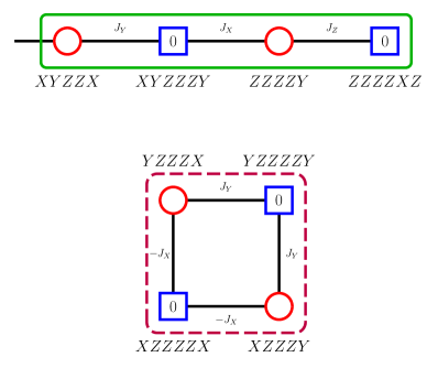
Figure 11: The graph visualisation showing the length $k=5$ Pauli string which is not a doubling-product operator has vanishing coefficient, while the doubling-product operator is included in ”Exception 2” case in the main text.

For the $XYZ$ model with magnetic fieldShiraishi (2019), the proof has been separated into two parts. First, it claims that every length $k$ Pauli strings which are not doubling-product operators have vanishing coefficient. Second, it claims that every doubling-product operators, which have linearly related coefficients, also have vanishing coefficient. Figure 11 shows that this fact can be visualized by using the subgraph of commutator graph. The graph above shows the promising path of the Pauli string $XYZZX$, which is not a doubling-product operator. The small coefficients $J_{X},J_{Y},$ and $J_{Z}$ above the edge is the coefficient of connected red circle. The graph below shows the loop containing the Pauli strings $YZZZX=\overline{YXYX}$ and $XZZZY=\overline{XYXY}$, which are both doubling-product operators.

Before going further, we introduce some modifications we can do on the commutator graph, which generates a new graph with completely same series of linear equations. This basically follows from the basic algebraic calculations on linear equations, as we can see below.

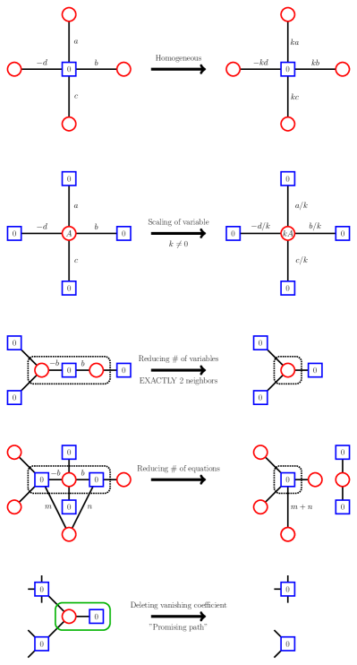
Figure 12: The graph modifications we can do on the commutator graph. First and second diagrams change the coefficients of the equations; third, fourth, and fifth diagrams reduces the number of parameters or equations.

Figure 12 shows the modifications. First diagram corresponds to the situation changing the equation $ax+by+cz-dw=0$ to $-2ax-2by-2cz+2dw=0$ by multiplying $2$ on both side; second diagram corresponds to the situation changing the parameter $A$ into $2A$. In the third diagram, the blue circle in the green box must have only two neighboring red circles, and then it corresponds to the situation when we have equation $-bx+by=0$ then $x=y$ so we can identify two red circles. Fourth diagram corresponds to the situation with two equations $ax-by+cz+mt=0$ and $by+dw+nt=0$, which reduces into the single equation $ax+cz+dw+(m+n)t=0$. The fifth diagram deletes the vanishing coefficient, which is equivalent to the ”promising path” argument in the main text. All these modifications are simple and complete to solve the serial linear equations, hence we may say that the modifications in Figure 12 is a complete method finding out the conserved quantity.

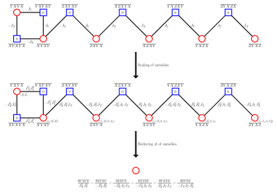
Figure 13: Showing every doubling-product operators have same coefficient, with appropriate scaling. At the first step, the modification in the second figure of 12 is used. At the second step, the modification in the third figure of 12 is used.

Using this method, we can argue the linear relations between coefficients of doubling-product operators. Figure 13 shows the result. First, by scaling the doubling-product operators by appropriate coefficients, change the edge coefficients so that every two edges on a blue circle have same absolute values but different signs. More precisely, scale the doubling-product operators as following: if $X,Y,$ and $Z$ appears $n_{X},n_{Y},$ and $n_{Z}$ times in doubling-product form respectively, then scale it by dividing with $J_{X}^{n_{X}}J_{Y}^{n_{Y}}J_{Z}^{n_{Z}}$, and if there are odd number of $XZ$, $ZY$, or $YX$ pairs in the doubling-product form, multiply $-1$. This modification of graph makes every blue circles in Figure 13 can be removed by the third diagram in Figure 12, which gives a single red circle.

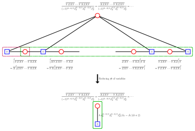
Figure 14: First figure shows the “quasi-double-promising path” of $k-1$ Pauli strings: two boxes represents two “quasi-promising paths” constructing a quasi-double-promising path. Using the fourth figure in Figure 12, we get the subgraph with blue circle having only one neighboring red circle, with non-zero edge coefficient(when $h\neq 0$ and $J_{X}\neq J_{Y}$ with $k\geq 6$). This shows the coefficients of every doubling-product operators vanish.

Now we have decided the coefficients every length $k$ Pauli strings, which however does not confirm the vanishing coefficient. To do this, we need to tackle the length $k-1$ Pauli strings. Notice that the commutator between length $k-1$ Pauli string and Hamiltonian might become length $k$ Pauli string, which can be also represented by the commutator between length $k$ Pauli string and Hamiltonian, hence this procedure must include the length $k$ Pauli strings also. Now we define the concept of quasi-promising path: if we erase a single vertex, then it becomes a promising path. Although the existence of a quasi-promising path do not implies the vanishing coefficient, the existence of two quasi-promising paths implies the vanishing coefficient: we say it a quasi-double-promising path(QDP path). The figure above in Figure 14 shows an example of QDP path in $XYZ+h$ model, where the ignoring red circle is a circle representing doubling-product operators. In this case, if we repetitively use the fourth figure in Figure 12(and the first figure in Figure 12 if needed, but not in this case), we get a simple subgraph with a blue circle which has only one neighboring red circle: a doubling-product operator. If the edge coefficient $hJ_{X}^{(k-2)/2}J_{Y}^{(k-4)/2}J_{Z}^{2}(J_{X}-J_{Y})(k+2)$ is nonzero(which is true in the setup), then we found the promising path, and showed every coefficients vanish.

From above argument, one can directly show that if we have a QDP path, then either the simplified graph have vanishing edge coefficient(in this case, the linear combination of every length $k$ Pauli strings might be included in a conserved quantity, which is the case with $h=0$: see Nozawa and Fukai (2020)), or the system have no conserved quantity. Notice that this “quasi-double-promising path” concept is applicable various models. Indeed, this concept is directly used when we show the zero coefficients in Appendix C and D, and is applicable when we visualize the proof of the nonintegrability of mixed-field Ising chain model which has been shown beforeChiba (2024). This concept is also quite natural and the simplest way, because in the case when we scanned every length $k$ operators, it is natural to scan every length $k-1$ operators.

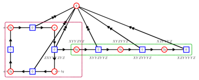
Figure 15: Graph representation of the proof of Theorem 7 in D. The left box represents “quasi-loop” which reduces into a “quasi-promising path”, and the right box represents another “quasi-promising path”. Notice that the two red circles marked with $q$ are the same circle, but for simplicity we drew them separately.

Although the existence of QDP path is critical to show the nonintegrability, and can be used in various other models including mixed-field Ising chainChiba (2024), not every commutator graph have QDP path. For example, in the PXP Hamiltonian, the proof of Theorem 7 does not use the QDP path directly: we first need to reduce “quasi-loop” on the left side into a quasi-promising path. See Fig.15 for details. However, since in this case the “quasi-loop” can be reduced into the quasi-promising path via the graph modifications in Fig.12, the usefulness of QDP path still holds here. We hence suggest that for general model, every Exception 2 case can be resolved by using the QDP path method.

References

- Rigol et al. (2007) M. Rigol, V. Dunjko, V. Yurovsky, and M. Olshanii, Phys. Rev. Lett. 98, 050405 (2007).
- Pozsgay (2013) B. Pozsgay, Journal of Statistical Mechanics: Theory and Experiment 2013, P07003 (2013).
- Vidmar and Rigol (2016) L. Vidmar and M. Rigol, Journal of Statistical Mechanics: Theory and Experiment 2016, 064007 (2016).
- Andrei (1980) N. Andrei, Phys. Rev. Lett. 45, 379 (1980).
- Zamolodchikov and Zamolodchikov (1978) A. B. Zamolodchikov and A. B. Zamolodchikov, Nuclear Physics B 133, 525 (1978).
- Coleman (1975) S. Coleman, Phys. Rev. D 11, 2088 (1975).
- Faddeev (1982) L. Faddeev, Integrable models in 1+ 1 dimensional quantum field theory, Tech. Rep. (CEA Centre d’Etudes Nucleaires de Saclay, 1982).
- Zhang et al. (2005) Y. Zhang, L. H. Kauffman, and M.-L. Ge, Quantum Information Processing 4, 159 (2005).
- Bethe (1931) H. Bethe, Zeitschrift für Physik 71, 205 (1931).
- Yang (1967) C.-N. Yang, Physical Review Letters 19, 1312 (1967).
- Baxter (1978) R. J. Baxter, Philosophical Transactions of the Royal Society of London. Series A, Mathematical and Physical Sciences 289, 315 (1978).
- Baxter (2016) R. J. Baxter, Exactly solved models in statistical mechanics (Elsevier, 2016).
- Takhtadzhan and Faddeev (1979) L. Takhtadzhan and L. D. Faddeev, Russian Mathematical Surveys 34, 11 (1979).
- Baxter (1972) R. J. Baxter, Annals of Physics 70, 323 (1972).
- Nozawa and Fukai (2020) Y. Nozawa and K. Fukai, Physical Review Letters 125, 090602 (2020).
- Shastry (1986) B. S. Shastry, Phys. Rev. Lett. 56, 2453 (1986).
- Fukai (2023) K. Fukai, Phys. Rev. Lett. 131, 256704 (2023).
- Feiguin et al. (2007) A. Feiguin, S. Trebst, A. W. W. Ludwig, M. Troyer, A. Kitaev, Z. Wang, and M. H. Freedman, Phys. Rev. Lett. 98, 160409 (2007).
- Casati et al. (1985) G. Casati, B. V. Chirikov, and I. Guarneri, Phys. Rev. Lett. 54, 1350 (1985).
- Grabowski and Mathieu (1995) M. P. Grabowski and P. Mathieu, Journal of Physics A: Mathematical and General 28, 4777 (1995).
- Shiraishi (2019) N. Shiraishi, Europhysics Letters 128, 17002 (2019).
- Chiba (2024) Y. Chiba, Phys. Rev. B 109, 035123 (2024).
- Bernien et al. (2017) H. Bernien, S. Schwartz, A. Keesling, H. Levine, A. Omran, H. Pichler, S. Choi, A. S. Zibrov, M. Endres, M. Greiner, et al., Nature 551, 579 (2017).
- Turner et al. (2018) C. J. Turner, A. A. Michailidis, D. A. Abanin, M. Serbyn, and Z. Papić, Nature Physics 14, 745 (2018).
- Alhambra et al. (2020) Á. M. Alhambra, A. Anshu, and H. Wilming, Physical Review B 101, 205107 (2020).
- Bull et al. (2020) K. Bull, J.-Y. Desaules, and Z. Papić, Phys. Rev. B 101, 165139 (2020).
- Bluvstein et al. (2021) D. Bluvstein, A. Omran, H. Levine, A. Keesling, G. Semeghini, S. Ebadi, T. T. Wang, A. A. Michailidis, N. Maskara, W. W. Ho, et al., Science 371, 1355 (2021).
- Su et al. (2023) G.-X. Su, H. Sun, A. Hudomal, J.-Y. Desaules, Z.-Y. Zhou, B. Yang, J. C. Halimeh, Z.-S. Yuan, Z. Papić, and J.-W. Pan, Phys. Rev. Res. 5, 023010 (2023).
- Desaules et al. (2024) J.-Y. Desaules, G.-X. Su, I. P. McCulloch, B. Yang, Z. Papić, and J. C. Halimeh, Quantum 8, 1274 (2024).
- Schecter and Iadecola (2019) M. Schecter and T. Iadecola, Phys. Rev. Lett. 123, 147201 (2019).
- Mark et al. (2020) D. K. Mark, C.-J. Lin, and O. I. Motrunich, Phys. Rev. B 101, 195131 (2020).
- Iadecola and Schecter (2020) T. Iadecola and M. Schecter, Phys. Rev. B 101, 024306 (2020).
- Note (1) If we include the Pauli strings with length , then there are various possible commutator representations of ; for example, . However, since is a length quantity, this kind of commutator does not appears in the calculation of , and thus we must ignore the cases like this.
- Note (2) Note that, independent to our work, the primitive concept of our promising path approach has been appeared in Ref.Fukai (2024), where the concept is systemized and applicable to general Hamiltonians in our work.
- Note (3) This happens because of the property of Pauli strings: Let and be a nonzero Pauli strings. If then .
- Note (4) Private communication with Prof. Hosho Katsura.
- Note (5) HaRu K. Park and SungBin Lee, in preparation.
- Note (6) Because , it is impossible to use the Hamiltonian string ; in this case, never becomes .
- Note (7) If or then the Pauli strings commute.
- Fukai (2024) K. Fukai, arXiv preprint arXiv:2402.08924 (2024).