Stable non-Fermi liquid fixed point at the onset of incommensurate $2k_{F}$ charge density wave order

Abstract

We consider the emergence of a non-Fermi liquid fixed point in two-dimensional metals at the onset of a quantum phase transition from a Fermi liquid state to an incommensurate charge density wave (CDW) ordered phase. The momentum of the CDW boson is centred at the wavevector $\bm{\mathcal{Q}}$, which connects a single pair of antipodal points on the Fermi surface with antiparallel tangent vectors. We employ the dimensional regularization technique in which the co-dimension of the Fermi surface is extended to a generic value, while keeping the dimension of Fermi surface itself fixed at one. Although the system is strongly coupled at dimension $d=2$, the interactions become marginal at the upper critical dimension $d=d_{c}$, whose value is found to be $5/2$. Using a controlled perturbative expansion in the parameter $\epsilon=d_{c}-d$, we compute the critical exponents of the stable infrared fixed point characterizing the quantum critical point. The scalings of the original theory are determined by setting $\epsilon=1/2$, where the fermion self-energy is seen to scale with the frequency with a fractional power law of $2/3$, which is the undisputed signature of a typical non-Fermi liquid phase.

I Introduction

While Landau’s Fermi liquid theory has been incredibly successful in describing normal metals, there exists an extensive number of metallic states where the framework fails. Although of widely different origins, these systems are widely known as non-Fermi liquids. A finite density of nonrelativistic fermions interacting with transverse $U(1)$ gauge field bosons was the first model, considered by Holstein et al. [1] to study the effects of the electromagnetic fields on a metal, to exhibit a non-Fermi liquid character. Subsequently, it was realized similar behaviour is found for finite-density fermions coupled with massless order parameter bosons at quantum critical points [2, 3, 4, 5, 6, 7, 8, 9, 10, 11, 12, 13, 14, 15, 16, 17, 18, 19, 20, 21, 22, 23, 24, 25, 26, 27, 28, 29, 30, 31] and artificial gauge field(s) emerging in various kinds of scenarios [32, 33, 34, 35, 36, 37, 38, 39]. While the Landau quasiparticles provide a natural single-particle basis for writing down low-energy quantum field theories (QFTs), on the merit of being long-lived excitations in a Landau Fermi liquid, they are destroyed by the strong interactions between the soft fluctuations of the Fermi surface and the gapless bosonic quantum fields in the scenarios described above. Since they are fundamentally strongly-interacting theories, it is a challenging task to build a controlled approximation amenable to theoretical analysis. As a result, there have been intensive efforts to devise QFT frameworks to explain the emergent physical characteristics of these non-Fermi liquid systems [1, 40, 35, 41, 42, 43, 39, 17, 44, 38, 7, 45, 25, 2, 26, 27, 46, 47, 48, 49, 50, 19, 28, 20, 21, 22, 23, 24, 29, 30, 31, 51, 52, 53, 54]. In two spatial dimensions, the corresponding theories are genuinely strongly interacting, while in three dimensions, they emerge as marginal Fermi liquids [20]. Analogous situations arise in two-dimensional (2d) and three-dimensional (3d) semimetals, where a non-Fermi liquid state emerges when the chemical potential cuts a band-crossing point giving rise to a Fermi point (rather than a Fermi surface) and a long-ranged (i.e., unscreened) Coulomb potential is switched on [55, 56, 57, 58, 59, 60, 61, 62, 63, 64].

For non-Fermi liquids arising at quantum critical points, there are two types of order parameter bosons: (1) cases where the critical bosonic field is centred about zero momentum, inducing the quasiparticles to lose coherence across the entire Fermi surface [2, 3, 4, 5, 6, 7, 8, 9, 10, 11, 12, 13, 14, 15, 16, 17, 18, 19, 20, 21, 22, 23, 24]; (2) the momentum of the quantum field describing the bosonic degrees freedom is centred around a finite vector equal to $\bm{\mathcal{Q}}$, which connects points on the Fermi surface (commonly known as hot-spots), such that the non-Fermi liquid behaviour emerges locally in the vicinity of the hot-spots [2, 26, 27, 28, 29, 30, 31, 52]. Examples in the first category include the Ising-nematic critical point, while the second one include ordering transitions to phases like spin density wave (SDW), charge density wave (CDW) [25, 26, 27, 28, 29, 30, 31], and the Fulde-Ferrell-Larkin-Ovchinnikov (FFLO) states [52]. A nonzero $\bm{\mathcal{Q}}$ vector can be a nesting vector of the Fermi surface, connecting two hot-spots with antiparallel tangent vectors, and with magnitude equal to $2\,k_{F}$, where $k_{F}$ is the local inverse curvature of the Fermi surface (i.e., the magnitude of the local Fermi momentum vector). We would like to emphasize that such a nesting vector causes a partial nesting of the Fermi surface, which is distinct from the perfect-nesting cases when slices (and not just discrete points) of a Fermi surface are connected by the same nesting vector.

In this paper, we consider a pair of antipodal points on a 1d Fermi surface (of a 2d metal) with parallel tangent vectors interacting with an order parameter boson, whose condensation gives rise to an incommensurate CDW ordered phase [65, 66, 67]. The CDW boson becomes massless right at the quantum critical point, giving rise to strong quantum fluctuations. The physical picture here is that the CDW boson drives the system across a quantum phase transition to an ordered state where the the electron density spontaneously breaks translational symmetries and develops a density modulation with a wave vector $\bm{\mathcal{Q}}$ that is incommensurate with the underlying reciprocal lattice vectors. For the sake of definiteness, we choose $\bm{\mathcal{Q}}=2\,k_{F}\,{\hat{\bm{x}}}$, without any loss of generality.

To deal with the QFT describing the above system, we implement the analytic approach of dimensional regularization [68, 19, 20, 21, 23, 22, 52, 53], in which the co-dimension of the Fermi surface is increased (as a mathematical tool) with the aim to obtain the value of the upper critical dimension $d=d_{c}$. Since $d_{c}$ is the dimension at which the interactions become marginal, we succeed in formulating a controlled perturbative approximation, although the quasiparticle-description has broken down. The critical exponents and various physical properties can now be calculated in a systematic expansion involving the perturbative parameter $\epsilon=d_{c}-2$. Halbinger et al. [67] have considered the incommensurate CDW problem, by employing the same methodology, and have found that the fermion-boson interactions lead to a stable non-Fermi liquid fixed point. Furthermore, their results show that the resulting critical Fermi surface is flattened at the hot-spots. However, they arrived at their conclusions from some inaccurate computations, which, in addition to other results, could not find the correct critical dimension $d_{c}=5/2$. Consequently, their answers do not include the all-important $\text{sgn}(k_{0})|k_{0}|^{2/3}$-dependence of the fermion self-energy, which is predicted in the earlier (uncontrolled) random phase approximation (RPA) calculations [65, 66]. In order to address these inadequacies, the analysis via the dimensional regularization scheme must be reexamined, if only to put it on a firmer basis.

The paper is organized as follows. In Sec. II, we introduce the effective low-energy action in the Matsubara frequency space, describing the fermionic excitations at the two hot-spots of the Fermi surface interacting with the CDW fluctuations. The original theory is embedded in $d=2$ spatial dimensions. We also explain how to generalize the theory to a generic value of $d$ by increasing the number of dimensions perpendicular to the 1d Fermi surface, as this will allow us to identify the upper critical dimension $d_{c}$ and, subsequently, to regularize the theory via the renormalization group (RG) procedure. Sec. III is devoted to the derivations of the bosonic and fermionic self-energies, and showing that $d_{c}$ comes out to be $5/2$. Using the one-loop results, the RG flow equations are determined in Sec. IV by absorbing the ultraviolet (UV) divergences into singular counterterms. We discuss the nature of the fixed points in the ifrared (IR) limit and show that the system flows to a stable non-Fermi liquid point. The values of the coupling constants at this stable fixed point lead to a flattening of the Fermi surface at the hot-spots. Finally, we conclude with the relevant discussions in Sec. V, comparing our computations and results with earlier works. The appendix shows a part of the computations of the fermion self-energy.

II Model

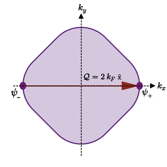
Figure 1: Schematics of the one-dimensional Fermi surface with two hot-spots connected by the wavevector $\bm{\mathcal{Q}}=2\,k_{F}\,\hat{\bm{x}}$ (indicated by the red arrow), which is incommensurate with the underlying reciprocal lattice vectors. The fermionic fields in the vicinity of the right and left hot-spots are designated as $\psi_{+}$ and $\psi_{-}$, respectively. They interact with the CDW order parameter bosonic fields whose momenta are centred at $\bm{\mathcal{Q}}$.

We consider the low-energy QFT action describing finite-density fermions confined to two spatial dimensions, and interacting with an incommensurate CDW order parameter with momentum centred at $\bm{\mathcal{Q}}=2\,k_{F}\,\hat{\bm{x}}$. Thus, the nesting vector $\bm{\mathcal{Q}}$ connects two hot-spots on the Fermi surface located along the $x$-axis. In $(2+1)$-dimensions, the effective action describing the electrons near the hot-spots and the CDW order parameter mode is given by [67, 65, 66]

$$S =\sum_{s=\pm}\int_{k}\psi_{s}^{\dagger}(k)\left(-i\,k_{0}+s\,k_{1}+k_{2}^{2}\right)\psi_{s}(k)+\int_{k}\phi_{+}(k)\left(k_{0}^{2}+k_{1}^{2}+k_{2}^{2}\right)\phi_{-}(-k)$$

$$\qquad+e\int_{k,q}\,\Big{[}\,\phi_{+}(q)\,\psi^{\dagger}_{+}(k+q)\,\psi_{-}(k)+\phi_{-}(-q)\,\psi^{\dagger}_{-}(k-q)\,\psi_{+}(k)\,\Big{]}\,,$$ (1)

where $k=(k_{0},\mathbf{k})$ denotes the three-vector comprising the Matsubara space frequency $k_{0}$ and the spatial momentum vector $\mathbf{k}=(k_{1},k_{2})$, $\int_{k}\equiv\int dk_{0}\,d^{d}{\mathbf{k}}/(2\,\pi)^{d+1}$, and $d=2$ is the number of spatial dimensions . The fermionic degrees of freedom about the right and left hot-spots are denoted by $\psi_{+}(k)$ and $\psi_{-}(k)$, respectively. The fields $\phi_{+}(k)$ and $\phi_{-}(k)$ refer to the bosonic fluctuations carrying frequency $k_{0}$ and momenta $\bm{\mathcal{Q}}/2+\mathbf{k}$ and $-\bm{\mathcal{Q}}/2+\mathbf{k}$, respectively. The boson is massless as we are considering the quantum critical point. To simplify notations, we have rescaled the fermionic momenta in a way such that the absolute value of the Fermi velocity is unity and the curvature of the Fermi surface is equal to $2$ at the hot-spots. Although the bosonic velocity is in general distinct from that of the fermions, we have set the bare velocity of the bosons to unity as well. This is because the dynamics of the bosons at the critical point is dominated by the particle-hole excitations of the Fermi surface at low energies, and the actual value of the bosonic velocity does not matter in the low-energy effective theory.

In our action, since the Fermi surface is locally parabolic, we can set the scaling dimensions of $k_{1}$ and $k_{2}$ are equal to $1$ and $1/2$, respectively. In order to extract the critical scalings in a controlled approximation, we increase the co-dimensions of the Fermi surface [68, 19, 28] and determine to determine the upper critical dimension $d=d_{c}$ where the fermion self-energy shows a logarithmic singularity. To preserve the analyticity of the theory in momentum space (alternatively, locality in real space) with generic co-dimensions, we introduce the two-component “spinors” [19, 20, 21, 52, 53, 54]

$$\Psi(k)=\left(\psi_{+}(k)\quad\psi_{-}^{\dagger}(-k)\right)^{T}\text{ and }\bar{\Psi}\equiv\Psi^{\dagger}\,\gamma_{0}\,,$$ (2)

and write an action that describes the 1d Fermi surface embedded in a $d$-dimensional momentum space:

$$S =\int_{k}\bar{\Psi}(k)\,i\left({\mathbf{\Gamma}}\cdot{\mathbf{K}}+\gamma_{d-1}\,\delta_{k}\right)\Psi(k)+\int_{k}\left(k_{d}^{2}+\tilde{a}\,e_{k}\right)\,\phi_{+}(k)\,\phi_{-}(-k)$$

$$\quad-\frac{i\,e\,\mu^{x_{e}/2}}{2}\int_{k,\,q}\Big{[}\,\phi_{+}(q)\,\bar{\Psi}(k+q)\,\gamma_{0}\,\bar{\Psi}^{T}(-k)+\phi_{-}(-q)\,\Psi^{T}(q-k)\,\gamma_{0}\,\Psi(k)\Big{]}\,,$$

$$x_{e} =\frac{5-2\,d}{2}\,,\quad\delta_{k}=k_{d-1}+k_{d}^{2}\,,\quad e_{k}=k_{d-1}+\frac{k_{d}^{2}}{2}\,.$$ (3)

The $(d-1)$-component vector ${\mathbf{K}}~{}\equiv~{}(k_{0},k_{1},\ldots,k_{d-2})$ includes the frequency and the $(d-2)$-components of the momentum vector due to the added co-dimensions, and the original momentum components along the $x$- and $y$-directions have been relabelled as $k_{d-1}$ and $k_{d}$, respectively. Hence, in the resulting $d$-dimensional momentum space, the set of components $\{k_{1},\cdots,k_{d-1}\}$ represents the $(d-1)$ the direction perpendicular to the Fermi surface, while $k_{d}$ is along the parallel direction. Similarly, the vector of matrices ${\mathbf{\Gamma}}\equiv(\gamma_{0},\gamma_{1},\ldots,\gamma_{d-2})$ has $(d-1)$ components representing the gamma matrices associated with $k_{0}$ and the extra co-dimensions. Ultimately we are interested in continuing to $d=2$, which implies that in practice we consider only the $2\times 2$ gamma matrices $\gamma_{0}=\sigma_{y}$ and $\gamma_{d-1}=\sigma_{x}$ in our computations.

In the purely bosonic part of the action, only the $k_{d}^{2}$ part of the kinetic term is retained, because $\left(|{\mathbf{K}}|^{2}+k_{d-1}^{2}\right)$ is irrelevant under the scaling of the patch-theory formalism [2, 19, 20, 21, 67, 52, 53], where each of $\left\{\mathbf{K},\,k_{d-1}\right\}$ has dimension unity and $k_{d}$ has dimension $1/2$. Dependence on $e_{k}$ in the bosonic propagator will be generated via the susceptibility, which is obtained from the dynamics of the strong particle-hole fluctuations. Anticipating this, we have already added the extra term $\tilde{a}\,e^{2}\,e_{k}$, which will be generated in the RG process, and its has been dictated by the divergent in the one-loop susceptibility calculated in the following subsection [see Eq. (13)]. In other words, we have simply included a term which will be generated via quantum corrections. This term has a mass dimension equal to unity, similar to the $k_{d}^{2}$ term, with a vanishing engineering dimension for $\tilde{a}$. If we do not include this term, the loop integrations involving the bosonic propagator will turn out to be infrared-divergent, and these divergences will be the mere artifacts of our dropping the irrelevant terms in the minimal local effective action (if it contains only the $k_{d}^{2}$ term). Finally, the engineering dimension of the fermion-boson coupling $e$ is equal to $x_{e}/2$ — this observation has dictated us to introduce an explicit factor of a mass scale $\mu^{x_{e}/e}$ chosen so as to ensure $e$ dimensionless, which is the usual procedure followed in quantum field theory calculations.

The emergent sliding symmetry in the Ising-nematic case [2, 19, 20, 21] forces the terms proportional to $\left[\bar{\Psi}(k)\,k_{d-1}\,\Psi(k)\right]$ and $\left[\bar{\Psi}(k)\,k_{d}^{2}\,\Psi(k)\right]$ in Eq. (II) to renormalize in the same way. In other words, the fermion propagator depends on $k_{d-1}$ and $k_{d}^{2}$ only through $\delta_{k}$ even after loop corrections. However, that is not the case here, and we will see that the renormalization process does not retain the sole dependence on $\delta_{k}$. In fact, the nature of the renormalized terms will be such that it leads to a flattening of the Fermi surface at the hot-spots, as found in the RPA calculations of Ref. [66].

III One-loop self-energies and dimensional regularization

The value of $x_{e}$ tells us that the coupling constant $e$ becomes marginal at the upper critical dimension $d_{c}=5/2$. In other words, $e$ is relevant for $d<5/2$ and irrelevant for $d>5/2$. Our aim is to access the interacting phase perturbatively in $d=5/2-\epsilon$, using $\epsilon$ as the perturbative parameter. In particular, this implies that at the end of our systematic $\epsilon$-expansion, we have to set $\epsilon=1/2$ for our original two-dimensional theory. Before embarking on deriving the RG flows, in this section, we compute the one-loop self-energies for the bosonic and fermionic degrees of freedom, which will feed into the equations necessary for determining the beta functions of the coupling constants $e$ and $\tilde{a}$.

The bare fermion and boson propagators for the action defined in Eq. (II) are given by

$$G_{(0)}(k) \equiv\left\langle\Psi(k)\,\bar{\Psi}(k)\right\rangle_{0}=\frac{1}{i}\,\frac{\mathbb{\Gamma}\cdot{\mathbf{K}}+\gamma_{d-1}\,\delta_{k}}{|\mathbf{K}|^{2}+\delta_{k}^{2}}\,,\quad D_{(0)}^{+}(k)\equiv\left\langle\phi^{+}(k)\phi^{-}(-k)\right\rangle_{0}=\frac{1}{k_{d}^{2}+\tilde{a}\,e_{k}}\,,$$

$$D_{(0)}^{-}(k) \equiv\left\langle\phi^{-}(k)\phi^{+}(-k)\right\rangle_{0}=D_{(0)}^{+}(k)(k)\,.$$ (4)

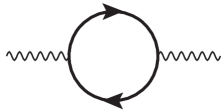
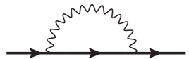
Figure 2: The one-loop diagrams for (a) the boson self-energy and (b) the fermion self-energy. Curves with arrows represent the bare fermion propagator $G_{(0)}$, whereas the wiggly lines represent the dressed bosonic propagator $D_{(1)}$.

III.1 One-loop boson self-energy

The one-loop boson self-energy [cf. Fig. 2] is defined by

$$\Pi(k)=-\frac{e^{2}\,\mu^{x_{e}}}{4}\times 2\int_{q}\text{Tr}\left[\gamma_{0}\,G_{(0)}(p)\,\gamma_{0}\,G_{(0)}^{T}(k-q)\right].$$ (5)

Using the commutation relations between the gamma-matrices, and the identities $\gamma_{d-1}^{T}=-\gamma_{0}\,\gamma_{d-1}\,\gamma_{0}$ and $\Gamma^{T}=-\gamma_{0}\,\Gamma\,\gamma_{0}$, we get

$$\Pi(k) =e^{2}\,\mu^{x_{e}}\int_{q}\frac{{\mathbf{Q}}\cdot({\mathbf{Q}}-{\mathbf{K}})-\delta_{q}\,\delta_{k-q}}{\left({\mathbf{Q}}^{2}+\delta_{q}^{2}\right)\left[({\mathbf{Q}}-{\mathbf{K}})^{2}+\delta_{k-q}^{2}\right]}\,.$$ (6)

Noting that $\delta_{k-q}=k_{d-1}+q_{d-1}+(k_{d}-q_{d})^{2}$, we first shift ${q}_{d-1}\rightarrow q_{d-1}-q_{d}^{2}$, and then use Feynman parametrization to obtain

$$\Pi(k) =e^{2}\,\mu^{x_{e}}\int_{q}\int_{0}^{1}dt\,\frac{|\mathbf{Q}|^{2}-t\,(1-t)\,|\mathbf{K}|^{2}-\tilde{e}_{kq}\,q_{d-1}+q_{d-1}^{2}}{\left[|\mathbf{Q}|^{2}+t\,(1-t)\,|\mathbf{K}|^{2}+t\,\tilde{e}_{kq}^{2}+q_{d-1}^{2}-2\,t\,\tilde{e}_{kq}\,q_{d-1}\right]^{2}}\quad\big{(}\text{where }\tilde{e}_{kq}=k_{d-1}+k_{d}^{2}-2\,k_{d}\,q_{d}+2\,q_{d}^{2}\big{)}$$

$$=e^{2}\,\mu^{x_{e}}\int d^{d-1}|\mathbf{Q}|\,dq\int_{0}^{1}dt\,\frac{|\mathbf{Q}|^{d}}{2^{d}\,\pi^{\frac{d+1}{2}}\,\Gamma\left(\frac{d-1}{2}\right)\left[|\mathbf{Q}|^{2}+t\,(1-t)\left(\tilde{e}_{kq}^{2}+|\mathbf{K}|^{2}\right)\right]^{3/2}}$$

$$=e^{2}\,\mu^{x_{e}}\int dq\,\frac{2^{1-2\,d}\csc\big(\frac{d\,\pi}{2}\big{missing})\left(\tilde{e}_{kq}^{2}+|\mathbf{K}|^{2}\right)^{\frac{d-2}{2}}}{\pi^{\frac{d-1}{2}}\,\Gamma\left(\frac{d-1}{2}\right)}\,.$$ (7)

Changing variables to $u=\sqrt{2}\,q_{d}-k_{d}/\sqrt{2}$ with the Jacobian factor $1/\sqrt{2}$, we get

$$\Pi(k) =e^{2}\,\mu^{x_{e}}\int_{0}^{\infty}du\,\frac{2^{\frac{3}{2}-2\,d}\csc\big(\frac{d\,\pi}{2}\big{missing})\left[\left(u^{2}+e_{k}\right)^{2}+|\mathbf{K}|^{2}\right]^{\frac{d-2}{2}}}{\pi^{\frac{d+1}{2}}\,\Gamma\left(\frac{d-1}{2}\right)}\,.$$ (8)

Since the bare susceptibility at zero temperature diverges at the nesting vector $\mathbf{Q}$, the well-defined self-energy is given by subtracting off the singular contribution for this momentum, which translates to

$$\tilde{\Pi}(k)=\Pi(k)-\Pi(0)=\frac{2^{\frac{3}{2}-2d}\csc\big(\frac{d\,\pi}{2}\big{missing})\,e^{2}\,\mu^{x_{e}}}{\pi^{\frac{d+1}{2}}\,\Gamma\left(\frac{d-1}{2}\right)}\,I_{\Pi}(k,d)\,,$$ (9)

where

$$I_{\Pi}(k,d) \equiv\int_{\tilde{e}_{k}}^{\infty}dz\,\frac{\left(z-{e_{k}}\right)^{2-d}-\left[z^{2}+|\mathbf{K}|^{2}\right]^{\frac{2-d}{2}}}{2\,\sqrt{z-{e_{k}}}\,\left[z^{2}+|\mathbf{K}|^{2}\right]^{\frac{2-d}{2}}\,\left(z-{e_{k}}\right)^{2-d}}$$

$$=\begin{cases}\frac{\Gamma(d-1)}{2\,\left(-{e_{k}}\right)^{3/2-d}}\left[\frac{\Gamma\left(\frac{3-d}{2}\right)\,\,_{2}F_{1}\left(\frac{3-2\,d}{4},\frac{5-2\,d}{4};\frac{3-d}{2};-\frac{|\mathbf{K}|^{2}}{{e_{k}}^{2}}\right)}{\sqrt{\pi}}+\frac{{}_{2}{F}_{1}\big{(}\frac{1}{2},1;d;1\big{)}}{\Gamma(d)}\right]&\\ +\frac{|\mathbf{K}|^{d}\,\,_{3}F_{2}\big{(}\frac{3}{4},1,\frac{5}{4};\frac{3}{2},\frac{d}{2}+1;-{|\mathbf{K}|^{2}}/{{e_{k}}^{2}}\big{)}}{4\,d\,\left(-{e_{k}}\right)^{3/2}}+\frac{\pi^{3/2}\,|\mathbf{K}|^{d-1}\sec\left(\frac{d\,\pi}{2}\right)\,\,_{2}{F}_{1}\big{(}\frac{1}{4},\frac{3}{4};\frac{d+1}{2};-{|\mathbf{K}|^{2}}/{{e_{k}}^{2}}\big{)}}{4\,\sqrt{-{e_{k}}}\,\,\Gamma\left(\frac{2-d}{2}\right)\,\Gamma\left(\frac{d+1}{2}\right)}&\\ +\,\frac{|\mathbf{K}|^{\frac{2\,d-5}{2}}}{\Gamma\left(\frac{2-d}{2}\right)}\bigg{[}|\mathbf{K}|\,\Gamma\left(\frac{5}{4}\right)\Gamma\left(\frac{3-d}{4}\right)\,_{2}F_{1}\big{(}\frac{1}{4},\frac{3-2\,d}{4};\frac{1}{2};-{e_{k}}^{2}/|\mathbf{K}|^{2}\big{)}&\\ +\,2\,\Gamma\left(\frac{3}{4}\right)\Gamma\left(\frac{5-d}{4}\right)\frac{\left\{(d-4)\,{\tilde{e}_{k}}^{2}-|\mathbf{K}|^{2}\right\}\,_{2}F_{1}\big{(}\frac{3}{4},\frac{1}{4}(5-2d);\frac{1}{2};-{e_{k}}^{2}/|\mathbf{K}|^{2}\big{)}\,+\,\left({e_{k}}^{2}+|\mathbf{K}|^{2}\right)\,_{2}F_{1}\big{(}\frac{3}{4},\frac{1}{4}(5-2d);-\frac{1}{2};-{{e_{k}}^{2}}/{|\mathbf{K}|^{2}}\big{)}}{(2\,d-3)\,{e_{k}}}\bigg{]}&\text{ for }{e_{k}}<0\\ &\\ \frac{\sqrt{\pi}\,e_{k}^{\frac{2\,d-3}{2}}\Gamma\left(\frac{3-d}{2}\right)\,\,_{2}F_{1}\big{(}\frac{3-2\,d}{4},\frac{5-2\,d}{4};\frac{3-d}{2};-|\mathbf{K}|^{2}/{{e_{k}}^{2}}\big{)}}{2\,\Gamma(2-d)}&\text{ for }e_{k}>0\,.\end{cases}$$ (10)

Note that the singular terms coming from $1/\Gamma(2-d)$ at $d=2$ are cancelled by the factor $\csc\big(\frac{d\,\pi}{2}\big{missing})$ present in Eq. (9).

The leading order terms obtained in the limit $|\mathbf{K}|^{2}/{e_{k}^{2}}\ll 1$ are found to be:

$$I_{\Pi}(k,d) =\begin{cases}\frac{\Gamma(d-1)}{2\,(-e_{k})^{\frac{3}{2}-d}}\left[\frac{{}_{2}\tilde{F}_{1}\big{(}\frac{1}{2},1;d;1\big{)}}{\Gamma(d)}+\frac{\Gamma\left(\frac{3-d}{2}\right)}{\sqrt{\pi}}\right]-\frac{\pi^{3/2}|\mathbf{K}|^{d-1}\sec\left(\frac{d\,\pi}{2}\right)}{4\,\sqrt{-e_{k}}\,\,\Gamma\left(\frac{2-d}{2}\right)\,\Gamma\left(\frac{d+1}{2}\right)}+\mathcal{O}\left(\frac{|\mathbf{K}|^{d}}{(-e_{k})^{3/2}}\right)&\text{ for }e_{k}<0\\ &\\ \frac{\sqrt{\pi}\,\Gamma\left(\frac{3}{2}-d\right)}{2\,\Gamma(2-d)\,e_{k}^{\frac{3}{2}-d}}+\frac{\sqrt{\pi}\,\Gamma\left(\frac{7}{2}-d\right)\,|\mathbf{K}|^{2}}{4\,(d-3)\,\Gamma(2-d)\,e_{k}^{\frac{7-2\,d}{2}}}+\mathcal{O}\left(\frac{|\mathbf{K}|^{4}}{e_{k}^{11/2-d}}\right)&\text{ for }e_{k}>0\,.\end{cases}$$ (11)

Finally, expanding in $\epsilon$ for $d=5/2-\epsilon$, we get

$$\left[\mu^{x_{e}}\,\frac{2^{\frac{3}{2}-2\,d}\csc\big(\frac{d\,\pi}{2}\big{missing})}{\pi^{\frac{d+1}{2}}\,\Gamma\left(\frac{d-1}{2}\right)}\times I_{\Pi}(k,d)\right]\Bigg{|}_{d=5/2-\epsilon}$$

$$=\begin{cases}-\frac{e_{k}\,\left(\frac{\mu}{|e_{k}|}\right)^{\epsilon}}{32\,\pi^{3/4}\,\Gamma\left(3/4\right)\,\epsilon}-\frac{3\,\pi+2\,\ln(32\,\pi)-2\,\gamma_{E}-12}{128\,\pi^{3/4}\,\Gamma\left(3/4\right)}\,e_{k}\,\left(\frac{\mu}{|e_{k}|}\right)^{\epsilon}+\frac{\pi^{3/4}\,\frac{|\mathbf{K}|^{\frac{3}{2}}}{\sqrt{|e_{k}|}}\,\,\left(\frac{\mu}{|\mathbf{K}|}\right)^{\epsilon}}{64\,\sqrt{2}\,\Gamma^{2}(3/4)\,\Gamma\left(7/4\right)}+\mathcal{O}\left(\epsilon\right)&\text{ for }e_{k}<0\\ &\\ -\frac{e_{k}\,\left(\frac{\mu}{e_{k}}\right)^{\epsilon}}{32\,\pi^{3/4}\,\Gamma\left(3/4\right)\,\epsilon}-\frac{3\,\pi\,+\,2\,\ln(32\,\pi)-2\,\gamma_{E}\,-4}{128\,\pi^{3/4}\,\Gamma\left(3/4\right)}\,e_{k}\,\left(\frac{\mu}{e_{k}}\right)^{\epsilon}-\frac{\frac{|\mathbf{K}|^{2}}{e_{k}}\,\,\left(\frac{\mu}{e_{k}}\right)^{\epsilon}}{32\,\pi^{3/4}\,\Gamma\left(3/4\right)}+\mathcal{O}\left(\epsilon\right)&\text{ for }e_{k}>0\,,\end{cases}$$ (12)

where $\gamma_{E}$ is the Euler–Mascheroni constant. It is important to note here that the loop integral has an upper critical dimension at $d=3/2$ and, as a result, it shows a pole in $\epsilon$ also at $d=5/2-\epsilon$. As such, these terms in the one-loop corrected action will be irrelevant, which is reflected by the that they have a scaling dimension equal to $(1-\epsilon)$ at $d=5/2-\epsilon$.

From our analysis above, we conclude that the self-energy correction in Eq. (15) is given by

$$\tilde{\Pi}(k)=-e^{2}\left[\frac{1}{32\,\pi^{3/4}\,\Gamma\left(3/4\right)\,\epsilon}+a\right]e_{k}-\frac{e^{2}\,\mu^{x_{e}}\,b\,|\mathbf{K}|^{d-1}}{\sqrt{|e_{k}|}}\,\Theta(-e_{k})+\frac{e^{2}\,c\,|\mathbf{K}|^{2}}{|e_{k}|^{7/2-d}}\,\Theta(e_{k})\,,$$ (13)

where

$$a =\frac{3\,\pi\,+\,2\,\ln(32\,\pi)-2\,\gamma_{E}\,-12}{64\,\pi^{3/4}\,\Gamma\left(3/4\right)}\,\Theta(-e_{k})+\frac{3\,\pi\,+\,2\,\ln(32\,\pi)-2\,\gamma_{E}\,-4}{64\,\pi^{3/4}\,\Gamma\left(3/4\right)}\,\Theta(e_{k})\,,$$

$$b =\frac{-\,\pi^{3/4}}{32\,\sqrt{2}\,\,\Gamma^{2}(3/4)\,\Gamma\left(7/4\right)}\,,\quad c=\frac{-\,1}{32\,\pi^{3/4}\,\Gamma\left(3/4\right)}\,.$$ (14)

We note that the bare boson propagators $D_{\pm}$ are still independent of $\mathbf{K}$, the loop integrations involving it are ill-defined unless one resums a series of diagrams that provides a nontrivial dispersion along these frequency and momentum components. Hence, in all loop calculations involving the boson propagators, we include the lowest order fine correction from the one-loop self-energy, which is proportional to $|\mathbf{K}|^{d-1}/\sqrt{|e_{k}|}$. Therefore, both for the $\phi_{+}(k)$ and $\phi_{-}(k)$ bosonic fields, we use the dressed propagator

$$D_{(1)}(k)=\frac{1}{k_{d}^{2}+\tilde{a}\,e_{k}+\frac{b\,e^{2}\,\mu^{x_{e}}\,|\mathbf{K}|^{d-1}\,\Theta(-e_{k})}{\sqrt{|e_{k}|}}}\,,$$ (15)

which is equivalent to rearranging the perturbative loop-expansions such that the one-loop finite part of the boson self-energy, dependent on $\mathbf{K}$, is included at the zeroth order. We also point out that this is the so-called Landau-damped term which leads to the signature $\text{sgn}(k_{0})|k_{0}|^{2/3}$-dependence of the fermion self-energy, characterizing the non-Fermi liquid behaviour in various quantum critical systems [2, 25, 19, 20, 21, 67, 52, 53]. The Landau-damped part also plays the most significant role in inducing unconventional superconductivity in this kind of non-Fermi liquid systems [48, 49, 69, 23, 24].

III.2 One-loop fermion self-energy

The fermion self-energy [cf. Fig. 2] is given by the integral

$$\Sigma(k) =e^{2}\,\mu^{x_{e}}\int_{q}\,\gamma_{0}\,G_{(0)}^{T}(q-k)\,\gamma_{0}\,D_{(1)}(q)=i\,\Sigma_{1}(k)\,\mathbf{\Gamma}\cdot\mathbf{K}+i\,\Sigma_{2}(k)\,\gamma_{d-1}\,,$$ (16)

where

$$\Sigma_{1}(k)=-\frac{e^{2}\,\mu^{x_{e}}}{|\mathbf{K}|^{2}}\int_{q}\frac{\mathbf{K}\cdot(\mathbf{Q}-{\mathbf{K}})}{(\mathbf{Q}-{\mathbf{K}})^{2}+\delta^{2}_{q-k}}\,D_{(1)}(q)$$ (17)

and

$$\Sigma_{2}(k)=e^{2}\,\mu^{x_{e}}\int_{q}\frac{\delta_{q-k}}{(\mathbf{Q}-{\mathbf{K}})^{2}+\delta^{2}_{q-k}}\,D_{(1)}(q)\,.$$ (18)

The steps to compute these two parts have been explained in the next two subsections, which can be skipped if the reader is not interested in the tedious intermediate steps. For their benefit, we state here the final result. Setting $d=d_{c}-\epsilon$, we get the UV-divergent part to be

$$\Sigma(k) =\left[-\frac{e^{4/3}\,\,{\mathcal{U}}_{1}\,}{\left(2-\tilde{a}\right)^{2/3}\,b^{1/3}\,\epsilon}+\order{\epsilon^{0}}\right]i\left(\mathbf{\Gamma}\cdot\mathbf{K}\right)+\frac{e^{2}\,\,{\mathcal{U}}_{2}\left[-e_{k}+\left(\frac{6+\tilde{a}}{2-\tilde{a}}\right)\frac{k_{d}^{2}}{2}\right]}{\left(2-\tilde{a}\right)\epsilon}\,,$$

$${\mathcal{U}}_{1} =\frac{\sqrt{2}\,\,\Gamma\big{(}\frac{5}{4}\big{)}}{3\,\sqrt{3}\,\pi^{7/4}}\,,\quad\,{\mathcal{U}}_{2}\,=\frac{\Gamma\big{(}\frac{5}{4}\big{)}}{2\,\sqrt{2}\,\pi^{7/4}}\,,$$ (19)

where the divergence is parametrized by a pole in $1/\epsilon$.

III.2.1 Computation of $\Gamma$-dependent part

The leading order dependence of $\Sigma_{1}(k)$ on $\mathbf{K}$ can be extracted by setting the external momentum components $k_{d}$ and $k_{d-1}$ to zero. Hence, we will evaluate

$$\Sigma_{1}(\mathbf{K},0,0)=\frac{e^{2}\,\mu^{x_{e}}}{|\mathbf{K}|^{2}}\int_{q}\frac{\mathbf{K}\cdot(\mathbf{K}-{\mathbf{Q}})}{(\mathbf{Q}-{\mathbf{K}})^{2}+\delta_{q}^{2}}\times\frac{1}{q_{d}^{2}+\tilde{a}\,e_{q}+e^{2}\,\mu^{x_{e}}\,b\,|\mathbf{Q}|^{d-1}\,\Theta(-e_{q})/\sqrt{|e_{q}|}}\,.$$ (20)

Changing the description to $q_{d}$ and $e_{q}$ as integration variables and dividing into the parts $e_{q}<0$ and $e_{q}>0$ as $\frac{|\mathbf{K}|^{2}\,\Sigma_{1}(\mathbf{K},0,0)}{e^{2}\,\mu^{x_{e}}}=I_{1}+I_{2}$, we have

$$I_{1} =\int_{e_{q}<0}\frac{d^{d-1}\mathbf{Q}\,dq_{d}\,de_{q}}{(2\,\pi)^{d+1}}\,\frac{-\mathbf{K}\cdot(\mathbf{Q}-\mathbf{K})}{(\mathbf{Q}-{\mathbf{K}})^{2}+\left(e_{q}+q_{d}^{2}/2\right)^{2}}\,\frac{1}{q_{d}^{2}+\tilde{a}\,e_{q}+e^{2}\,\mu^{x_{e}}\,b\,|\mathbf{Q}|^{d-1}/\sqrt{|e_{q}|}}$$

$$=\int_{0}^{\infty}\frac{du}{\sqrt{u/2}}\int_{0}^{\infty}de_{q}\int_{-\infty}^{\infty}\frac{d^{d-1}\mathbf{Q}}{(2\,\pi)^{d+1}}\,\frac{\mathbf{K}^{2}-\mathbf{K}\cdot\mathbf{Q}}{(\mathbf{Q}-{\mathbf{K}})^{2}+\left(u-e_{q}\right)^{2}}\,\frac{1}{2\,u-\tilde{a}\,e_{q}+e^{2}\,\mu^{x_{e}}\,b\,|\mathbf{Q}|^{d-1}/\sqrt{e_{q}}}\quad\left[\text{where }2\,u={q_{d}^{2}}\right]$$ (21)

and

$$I_{2} =\int_{e_{q}>0}\frac{d^{d-1}\mathbf{Q}\,dq_{d}\,de_{q}}{(2\,\pi)^{d+1}}\,\frac{-\mathbf{K}\cdot(\mathbf{Q}-\mathbf{K})}{(\mathbf{Q}-{\mathbf{K}})^{2}+\left(e_{q}+q_{d}^{2}/2\right)^{2}}\,\frac{1}{q_{d}^{2}+\tilde{a}\,e_{q}}$$

$$=\int_{e_{q}>0}\frac{d^{d-1}\mathbf{Q}\,dq_{d}\,de_{q}}{(2\,\pi)^{d+1}}\,\frac{-\mathbf{K}\cdot\mathbf{Q}}{\mathbf{Q}^{2}+\left(e_{q}+q_{d}^{2}/2\right)^{2}}\,\frac{1}{q_{d}^{2}+\tilde{a}\,e_{q}}=0\,.$$ (22)

The integral $I_{1}$ cannot be evaluated exactly and we need to make some reasonable approximations to extract the leading order corrections. We note that the first factor of the integrand tells us that the dominant contribution is concentrated around the region $|\mathbf{Q}|\sim|\mathbf{K}|$ and $u\sim e_{q}$. As for the second factor, the dominant contribution comes from $e_{q}\sim|\mathbf{Q}|^{2\,(d-1)/3}\sim|\mathbf{K}|^{2\,(d-1)/3}$. Since $|\mathbf{K}|^{2\,(d-1)/3}\gg|\mathbf{K}|$, we can substitute $u\sim e_{q}$ in the $\sqrt{u}$ factor in the overall denominator and the $2\,u$ term in the denominator of the second factor, and extend the lower limit of the integral over $u$ to $-\infty$, leading to

$$I_{1} \simeq\int_{-\infty}^{\infty}\frac{d^{d-1}\mathbf{Q}\,du}{(2\,\pi)^{d+1}}\int_{e_{q}>0}\frac{de_{q}}{\sqrt{e_{q}/2}}\,\frac{\mathbf{K}\cdot(\mathbf{K}-{\mathbf{Q}})}{(\mathbf{Q}-{\mathbf{K}})^{2}+u^{2}}\,\frac{1}{\left(2-\tilde{a}\right)e_{q}+e^{2}\,\mu^{x_{e}}\,b\,|\mathbf{Q}|^{d-1}/\sqrt{e_{q}}}\quad\left[\text{shifting }u\rightarrow u+e_{q}\right]$$

$$=\int_{-\infty}^{\infty}\frac{d^{d-1}\mathbf{Q}\,du}{(2\,\pi)^{d+1}}\int_{e_{q}>0}de_{q}\,\frac{\mathbf{K}\cdot(\mathbf{K}-{\mathbf{Q}})}{(\mathbf{Q}-{\mathbf{K}})^{2}+u^{2}}\,\frac{\sqrt{2}}{\left(2-\tilde{a}\right)e_{q}^{3/2}+e^{2}\,\mu^{x_{e}}\,b\,|\mathbf{Q}|^{d-1}}$$

$$=-\frac{e^{4/3}\,\Gamma\big{(}\frac{5-2d}{6}\big{)}\,\Gamma\big{(}\frac{d}{2}\big{)}\,\Gamma\big{(}\frac{d+2}{6}\big{)}}{2^{\frac{4d-1}{6}}\pi^{\frac{d+1}{2}}\times 3\,\sqrt{3}\left(2-\tilde{a}\right)^{2/3}\,b^{1/3}\,\Gamma\big{(}\frac{5d-2}{6}\big{)}}\left(\frac{\mu}{|\mathbf{K}|}\right)^{\frac{2\,x_{e}}{3}}\,.$$ (23)

The integral blows up at $d=5/2$, which thus gives us the value of the upper critical dimension $d_{c}$. The fermion-boson coupling $e$ is irrelevant for $d>d_{c}$, relevant for $d<d_{c}$, and marginal for $d=d_{c}$. This allows us to access the strongly interacting non-Fermi liquid state perturbatively, in a controlled approximation, using $d=5/2-\epsilon$, where $\epsilon$ serves as the perturbative parameter small parameter. In our dimensional regularization scheme, the divergence appears as $\sim\epsilon^{-1}$, with the $\Gamma(5d-2)$ factor having a pole at $d=d_{c}$. We also note that this term produces the behaviour of the fermion self-energy as $\sim\text{sgn}(k_{0})\,|k_{0}|^{2/3}$ at $d=2$, which matches with the uncontrolled RPA result [65, 66]. We would like to point out that the correct $k_{0}$-dependence of $\Sigma$ could be captured only because we have included the crucial Landau damping term in the dressed bosonic propagator $D_{(1)}$. This was missed in Ref. [67] due to the non-inclusion of this term.

III.2.2 Computation of $\gamma$-dependent part

The leading order dependence of $\Sigma_{2}(k)$ on $k_{d}$ and $k_{d-1}$ can be extracted by setting $\mathbf{K}=0$ to zero. Hence, we will evaluate

$$\Sigma_{2}(\mathbf{0},k_{d},k_{d-1}) =e^{2}\,\mu^{x_{e}}\,I_{3}\,,\quad I_{3}=\int_{q}\frac{\delta_{q-k}}{\mathbf{Q}^{2}+\delta^{2}_{q-k}}\times\frac{1}{q_{d}^{2}+\tilde{a}\,e_{q}+e^{2}\,\mu^{x_{e}}\,b\,|\mathbf{Q}|^{d-1}\,\Theta(-e_{q})/\sqrt{|e_{q}|}}\,,$$ (24)

where $\delta_{q-k}=q_{d-1}-k_{d-1}+k_{d}^{2}+q_{d}^{2}-2\,k_{q}\,q_{d}$. We note that the first factor of the integrand sets the condition that the dominant contributions must come when $|\mathbf{Q}|\sim 0$. This immediately tells us in the denominator of the second factor, the term proportional to $b$ is subleading. Hence, to extract the leading order contribution we can set to zero. In the appendix, we show that the subleading order term turns out to be proportional to $b^{1/3}$ and is not singular at $d=d_{c}$. Therefore, we calculate the approximate integral

$$I_{3} \simeq\int_{q}\frac{\delta_{q-k}}{\mathbf{Q}^{2}+\delta^{2}_{q-k}}\times\frac{1}{q_{d}^{2}+\tilde{a}\,e_{q}}$$

$$=\int\frac{d^{d-1}\mathbf{Q}\,dq_{d}\,du}{(2\,\pi)^{d+1}}\frac{u-k_{d-1}}{\left[|\mathbf{Q}|^{2}+\left(u-k_{d-1}\right)^{2}\right]\left(2-\tilde{a}\right)}\times\frac{2}{q_{d}^{2}+\frac{2\,\tilde{a}}{2-\tilde{a}}\left(u-2\,k_{d}\,q_{d}-k_{d}^{2}\right)}\quad[\text{where }u=\delta_{q}+2\,k_{d}\,q_{d}+k_{d}^{2}]\,.$$ (25)

Using the identity

$$\int_{-\infty}^{\infty}\frac{dw}{w^{2}+A}=\begin{cases}0&\text{ for }\mathcal{A}<0\\ \frac{\pi}{\sqrt{\mathcal{A}}}&\text{ for }\mathcal{A}>0\,,\end{cases}$$ (26)

for the Cauchy principle value, the $q_{d}$-integral is performed first to obtain the form

$$I_{3} =\int\frac{d^{d-1}\mathbf{Q}\,du}{(2\,\pi)^{d}}\frac{u-k_{d-1}}{\left[|\mathbf{Q}|^{2}+\left(u-k_{d-1}\right)^{2}\right]}\times\frac{\Theta\big{(}u-\frac{\left(2+\tilde{a}\right)\,k_{d}^{2}}{2-\tilde{a}}\big{)}}{\left(2-\tilde{a}\right)\sqrt{u-\frac{\left(\tilde{a}+2\right)k_{d}^{2}}{2-\tilde{a}}}}$$

$$=\int\frac{d^{d-1}\mathbf{Q}\,du}{(2\,\pi)^{d}}\frac{\frac{\left(2+\tilde{a}\right)\,k_{d}^{2}}{2-\tilde{a}}+\tilde{u}-k_{d-1}}{\left[|\mathbf{Q}|^{2}+\left(\frac{\left(\tilde{a}+2\right)\,k_{d}^{2}}{2-\tilde{a}}+\tilde{u}-k_{d-1}\right)^{2}\right]}\times\frac{\Theta(\tilde{u})}{\left(2-\tilde{a}\right)\sqrt{\tilde{u}}}\quad[\text{where }\tilde{u}=u-\frac{\left(2+\tilde{a}\right)\,k_{d}^{2}}{2-\tilde{a}}]$$

$$=\int_{0}^{\infty}\frac{d|\mathbf{Q}|}{\pi^{\frac{d-1}{2}}}\,\frac{1}{2^{d}\,\sqrt{2-\tilde{a}}\,\,\Gamma\big{(}\frac{d-1}{2}\big{)}\,|\mathbf{Q}|^{2-d}}\left[\frac{1}{\sqrt{\left(2+\tilde{a}\right)\,k_{d}^{2}-\left(2-\tilde{a}\right)\left(k_{d-1}+i\,|\mathbf{Q}|\right)}}+\frac{1}{\sqrt{\left(2+\tilde{a}\right)\,k_{d}^{2}+\left(2-\tilde{a}\right)\left(-k_{d-1}+i\,|\mathbf{Q}|\right)}}\right]$$

$$=\frac{\sin\big(\frac{\pi\,d}{2}\big{missing})\,\Gamma\big{(}\frac{3}{2}-d\big{)}\,\Gamma\big{(}\frac{d}{2}\big{)}}{2\,\pi^{\frac{d+1}{2}}\left(2-\tilde{a}\right)^{d+\frac{1}{2}}}\,\left[-e_{k}+\left(\frac{6+\tilde{a}}{2-\tilde{a}}\right)\frac{k_{d}^{2}}{2}\right]^{d-\frac{3}{2}}$$ (27)

Th factor $\Gamma\big{(}\frac{3}{2}-d\big{)}$ has a pole at $d=3/2$, which obviously shows it has poles for $d=5/2,\,7/2,\cdots$ as well. Therefore, at $d=d_{c}-\epsilon$, we have

$$\Sigma_{2}=\frac{e^{2}\,\,{\mathcal{U}}_{2}\left[-e_{k}+\left(\frac{6+\tilde{a}}{2-\tilde{a}}\right)\frac{k_{d}^{2}}{2}\right]}{\left(2-\tilde{a}\right)\epsilon}\left[\frac{\mu}{-e_{k}+\left(\frac{6+\tilde{a}}{2-\tilde{a}}\right)\frac{k_{d}^{2}}{2}}\right]^{\epsilon}+\order{\epsilon^{0}}\text{ where }{\mathcal{U}}_{2}=\frac{\Gamma\big{(}\frac{5}{4}\big{)}}{2\,\sqrt{2}\,\pi^{7/4}}\,.$$ (28)

III.3 One-loop vertex correction

It is not possible to get a one-loop vertex diagram and, hence, the corresponding correction is zero.

IV Renormalization Group flows under minimal subtraction scheme

Eq. (II) is supposed to be the physical action, defined at an energy scale $\mu$, consisting of the fundamental Lagrangian with non-divergent quantities. However, we have seen that loop integrals lead to divergent terms and, in order to cure it, we employ the renormalization procedure, using dimensional regularization as the regularization method. In our dimensional regularization formalism, the UV-divergent terms are the ones arising in the $\epsilon\rightarrow 0$ limit. We use the minimal subtraction (${\rm MS}$) renormalization scheme to control the UV divergences [70, 71], which involves cancelling the divergent parts of the loop-contributions via adding appropriate counterterms. More precisely, we adopt the modified minimal subtraction ($\overline{\rm MS}$) scheme, where, in addition to the divergent term, we absorb the universal term proportional to $\epsilon^{0}$ (that always accompanies the term with the $1/\epsilon$ pole), into the corresponding counterterm.

The action consisting of the counterterms to absorb the singular terms takes the form:

$$S_{CT}= \int_{k}\bar{\Psi}(k)\,i\,\Bigl{[}A_{1}\,{{\mathbf{\Gamma}}}\cdot{{\mathbf{K}}}+\gamma_{d-1}\left(A_{2}\,e_{k}+A_{3}\,\frac{k_{d}^{2}}{2}\right)\Bigr{]}\Psi(k)+\int_{k}\left(A_{4}\,k_{d}^{2}+A_{5}\,\tilde{a}\,e_{k}\right)\phi_{+}(k)\,\phi_{-}(-k)$$

$$\,-\frac{i\,e\,\mu^{x_{e}/2}}{2}\int_{k,\,q}A_{6}\,\Big{[}\,\phi_{+}(q)\,\bar{\Psi}(k+q)\,\gamma_{0}\,\bar{\Psi}^{T}(-k)+\phi_{-}(-q)\,\Psi^{T}(q-k)\,\gamma_{0}\,\Psi(k)\Big{]}\,.$$ (29)

The counterterm-factors are given by power series

$$A_{\zeta}=\sum_{n=1}^{\infty}\frac{Z^{(n)}_{\zeta}}{\epsilon^{n}}\text{ with }\zeta\in[1,6]\,,$$ (30)

such that they cancel the divergent $1/\epsilon^{n}$ contributions from the Feynman diagrams. Due to the $(d-1)$-dimensional rotational invariance in the space perpendicular to the Fermi surface, each term in ${{\mathbf{\Gamma}}}\cdot{{\mathbf{K}}}$ is renormalized in the same way.

Adding $S_{CT}$ to $S_{\text{bare}}$, we obtain the renormalized action, which is the physical effective action of the theory, re-written in terms of non-divergent quantum parameters. While the bare parameters can be divergent, the physical observables are the renormalized coupling constants, which are determined by the RG equations. The RG flows describes the evolution of the bare couplings as a function of the floating energy scale $\mu\,e^{-l}$. To achieve this objective, we first define the bare (or fundamental) action

$$S_{\text{bare}}= \int_{k^{B}}\bar{\Psi}^{B}(k^{B})\,\,i\left[\,{{\mathbf{\Gamma}}}\cdot{{\mathbf{K}}^{B}}+\gamma_{d-1}\left\{e_{k}^{B}+\frac{\left(k^{B}\right)^{2}}{2}\right\}\right]\Psi^{B}(k^{B})+\int_{k^{B}}\left[\left(k^{B}_{d}\right)^{2}+\alpha^{B}\,e_{k}^{B}\right]\phi_{+}^{B}(k^{B})\,\,\phi_{-}^{B}(-k^{B})$$

$$\,-\frac{i\,e^{B}}{2}\int_{k^{B},\,\,q^{B}}\Big{[}\,\phi^{B}_{+}(q^{B})\,\bar{\Psi}^{B}(k^{B}+q^{B})\,\gamma_{0}\left({\bar{\Psi}}^{B}(-k^{B})\right)^{T}+\phi^{B}_{-}(-q^{B})\left({\Psi^{B}}(q^{B}-k^{B})\right)^{T}\gamma_{0}\,\Psi^{B}(k^{B})\Big{]}\,,$$ (31)

consisting of the bare quantities, where the superscript “$B$” has been used to denote the bare fields, couplings, frequency, and momenta. We now relate the bare quantities to so-called renormalized quantities (without the superscript “$B$”) via the multiplicative $Z_{\zeta}$-factors such that

$$S_{\text{bare}}= S+S_{CT}\,,\quad Z_{\zeta}=1+A_{\zeta}\,,$$ (32)

$${{\mathbf{K}}}^{B}=\frac{Z_{1}}{Z_{3}}\,{{\mathbf{K}}}\,,\quad e_{k}^{B}=\frac{Z_{2}}{Z_{3}}\,e_{k}\,,\quad k^{B}_{d}=k_{d}\,,\quad\Psi^{B}(k^{B})=Z_{\Psi}^{1/2}\,\Psi(k)\,,\quad\phi_{\pm}^{B}(k^{B})=Z_{\phi}^{1/2}\,\phi_{\pm}\,,$$ (33)

and

$$Z_{\Psi}=Z_{1}\left(\frac{Z_{1}}{Z_{3}}\right)^{-d}\left(\frac{Z_{2}}{Z_{3}}\right)^{-1},\quad Z_{\phi}=Z_{4}\left(\frac{Z_{1}}{Z_{3}}\right)^{1-d}\left(\frac{Z_{2}}{Z_{3}}\right)^{-1},\quad{\tilde{a}}^{B}=Z_{5}\left(\frac{Z_{1}}{Z_{3}}\right)^{1-d}\left(\frac{Z_{2}}{Z_{3}}\right)^{-2},$$

$$e^{B}=Z_{e}\,e\,\mu^{\frac{\epsilon}{2}}\,,\quad Z_{e}=\frac{Z_{7}\left(\frac{Z_{1}}{Z_{3}}\right)^{1-\frac{d}{2}}\,\left({\frac{Z_{2}}{Z_{3}}}\right)^{-1/2}}{\sqrt{Z_{1}}\,Z_{4}}\,.$$ (34)

Observing that thee exists a freedom to change the renormalization of the fields and the renormalization of momenta without affecting the action, we have exploited this fact by requiring $k^{B}_{d}=k_{d}$, which is equivalent to measuring the scaling dimensions of all other quantities relative to that of $k_{d}$. $S$ now represents the renormalized active (also known as the Wilsonian effective action) because it consists of the renormalized quantities. Basically, we have written the fundamental action of our theory in two different ways [72], which allows us to subtract off the divergent parts (represented by $S_{CT}$).

IV.1 RG flow equations from one-loop results

At one-loop order, the divergent contributions are obtained from Eqs.(13) and (19). These lead to

$$Z_{1} =1-\frac{e^{4/3}\,\,{\mathcal{U}}_{1}\,}{\left(2-\tilde{a}\right)^{2/3}b^{1/3}\,\epsilon}\,,\quad Z_{2}=1-\frac{e^{2}\,\,{\mathcal{U}}_{2}\,}{\left(2-\tilde{a}\right)\epsilon}\,,\quad Z_{3}=1+\frac{e^{2}\left(6+\tilde{a}\right)\,{\mathcal{U}}_{2}\,}{\left(2-\tilde{a}\right)^{2}\,\epsilon}\,,\quad Z_{4}=1\,,\quad Z_{5}=1-\frac{e^{2}\,\,{\mathcal{U}}_{3}\,}{a\,\epsilon}\,,\quad Z_{6}=1\,,$$

$$b =\frac{-\,\pi^{3/4}}{32\,\sqrt{2}\,\,\Gamma^{2}\big{(}3/4\big{)}\,\Gamma\left(7/4\right)}\,,\quad{\mathcal{U}}_{1}=\frac{\sqrt{2}\,\,\Gamma\big{(}\frac{5}{4}\big{)}}{3\,\sqrt{3}\,\pi^{7/4}}\,,\quad\,{\mathcal{U}}_{2}\,=\frac{\Gamma\big{(}\frac{5}{4}\big{)}}{2\,\sqrt{2}\,\pi^{7/4}}\,,\quad\,{\mathcal{U}}_{3}\,=\frac{1}{32\,\pi^{3/4}\,\Gamma\left(3/4\right)}\,.$$ (35)

We define the quantities

$$z=1+\frac{\partial\ln\big(\frac{Z_{1}}{Z_{3}}\big{missing})}{\partial\ln\mu}\text{ and }\tilde{z}=1+\frac{\partial\ln\big(\frac{Z_{1}}{Z_{2}}\big{missing})}{\partial\ln\mu}\,,$$ (36)

where $z$ is the dynamical critical exponent for the fermions with respect to $e_{k}$. Furthermore, the anomalous dimensions for the fermions and bosons are given by

$$\eta_{\psi}=\frac{1}{2}\frac{\partial\ln Z_{\psi}}{\partial\ln\mu}\text{ and }\eta_{\phi}=\frac{1}{2}\frac{\partial\ln Z_{\phi}}{\partial\ln\mu}\,,$$ (37)

respectively. We also define the beta functions for the two various coupling constants as

$$\beta_{e}=\frac{de}{d\ln\mu}\text{ and }\beta_{a}=\frac{d\tilde{a}}{d\ln\mu}\,.$$ (38)

The sole purpose of the ad hoc mass scale $\mu$ is to regularize the theory to avoid the infinities emerging from the loop integrals of Feynman diagrams. However, physical quantities must be independent of $\mu$ as it is not really a parameter of the fundamental theory, the bare parameters must be independent of it as well. Imposing this condition, as well as the requirement that the regular (i.e., non-singular) parts of the final solutions are of the forms

$$z=z^{(0)}\,,\quad\tilde{z}=\tilde{z}^{(0)}\,,\quad\eta_{\psi}=\eta_{\psi}^{(0)}+\eta_{\psi}^{(1)}\,\epsilon\,,\quad\eta_{\phi}=\eta_{\phi}^{(0)}+\eta_{\phi}^{(1)}\,\epsilon\,,\quad\beta_{e}=\beta_{e}^{(0)}+\beta_{e}^{(1)}\,\epsilon\,,\quad\beta_{a}=\beta_{a}^{(0)}+\beta_{a}^{(1)}\,\epsilon\,,$$ (39)

in the limit $\epsilon\rightarrow 0$, we get the following differential equations:

$$z =1+\beta_{a}^{(1)}\left(\frac{\partial Z_{1}^{(1)}}{\partial\tilde{a}}-\frac{\partial Z_{3}^{(1)}}{\partial\tilde{a}}\right)+\beta_{e}^{(1)}\left(\frac{\partial Z_{1}^{(1)}}{\partial e}-\frac{\partial Z_{3}^{(1)}}{\partial e}\right),\quad\tilde{z}=1+\beta_{a}^{(1)}\left(\frac{\partial Z_{2}^{(1)}}{\partial\tilde{a}}-\frac{\partial Z_{3}^{(1)}}{\partial\tilde{a}}\right)+\beta_{e}^{(1)}\left(\frac{\partial Z_{2}^{(1)}}{\partial e}-\frac{\partial Z_{3}^{(1)}}{\partial e}\right),$$

$$\eta_{\psi} =\frac{1}{4}\left(7-5\,z-2\,\tilde{z}+2\,\frac{\partial Z_{1}^{(1)}}{\partial\tilde{a}}\,\,\beta_{a}^{(1)}+2\,\frac{\partial Z_{1}^{(1)}}{\partial e}\,\beta_{e}^{(1)}\right)+\frac{(z-1)\,\epsilon}{2}\,,\quad\eta_{\phi}=\frac{5-3\,z-2\,\tilde{z}}{4}+\frac{(z-1)\,\epsilon}{2}\,,$$

$$\frac{4\,\beta_{e}^{(0)}}{e} =2\left(\frac{\partial Z_{1}^{(1)}}{\partial\tilde{a}}\,\beta_{a}^{(1)}+\tilde{z}-1\right)-e\,z\,\frac{\partial Z_{1}^{(1)}}{\partial e}+z-1\,,\quad\,,\quad\beta_{e}^{(1)}=-\frac{e\,z}{2}\,,$$

$$\frac{2\,\beta_{a}^{(0)}}{\tilde{a}} =(z-1)\left(3+2\,\tilde{a}\,\frac{\partial Z_{5}^{(1)}}{\partial\tilde{a}}\right)+4\left(\tilde{z}-1\right)-2\,\frac{\partial Z_{5}^{(1)}}{\partial e}\,\beta_{e}^{(1)}\,,\quad\beta_{a}^{(1)}=-\tilde{a}\left(z-1\right)\,,$$ (40)

The above set of equations have been obtained by (1) demanding that $\frac{d}{d\ln\mu}\,(\mbox{bare quantity})=0$; (2) plugging in the values from Eqs. (IV.1) and (39); (3) expanding in powers of $\epsilon$; and (4) matching the coefficients of the regular powers of $\epsilon$ in the resulting equations.

Solving the equations, we get

$$\frac{-4\,\beta_{e}^{(0)}}{e}=\frac{3\,{\mathcal{U}}_{2}\,\chi^{-1/3}\,\tilde{e}^{3/2}\left[88-4\,\tilde{a}\left(4\,{\mathcal{U}}_{2}\,\tilde{e}^{3/2}+21\right)+\tilde{a}^{3}+18\,\tilde{a}^{2}\right]+6\,{\mathcal{U}}_{1}\,\chi^{3}\,\tilde{e}}{\tilde{a}^{2}\left[4\,{\mathcal{U}}_{1}\,\tilde{e}-18\,\chi^{2/3}\right]+4\left[9\,{\mathcal{U}}_{2}\,\chi^{2/3}\,\tilde{e}^{3/2}-6\,\chi^{2/3}+4\,{\mathcal{U}}_{1}\tilde{e}\right]+2\,\tilde{a}\left[15\,{\mathcal{U}}_{2}\,\chi^{2/3}\,\tilde{e}^{3/2}+18\,\chi^{2/3}-8\,{\mathcal{U}}_{1}\tilde{e}\right]+3\,\tilde{a}^{3}\chi^{2/3}}\,,$$ (41)

$$\frac{-2\,\beta_{e}^{1}}{e}=\frac{3\,\chi^{3}\left[\frac{\,{\mathcal{U}}_{2}\,\tilde{a}\left(\tilde{a}+14\right)\tilde{e}^{3/2}}{\chi^{3}}+\frac{2\,{\mathcal{U}}_{1}\,\tilde{a}\,\tilde{e}}{3\,\chi^{5/3}}-1\right]}{6\,{\mathcal{U}}_{2}\,\left(5\,\tilde{a}+6\right)\tilde{e}^{3/2}-4\,{\mathcal{U}}_{1}\,\chi^{1/3}\,\tilde{a}\,\tilde{e}+8\left({\mathcal{U}}_{1}\,\chi^{1/3}\,\tilde{e}-3\right)+3\,\tilde{a}\left[12-\left(6-\tilde{a}\right)\tilde{a}\right]}\,,$$ (42)

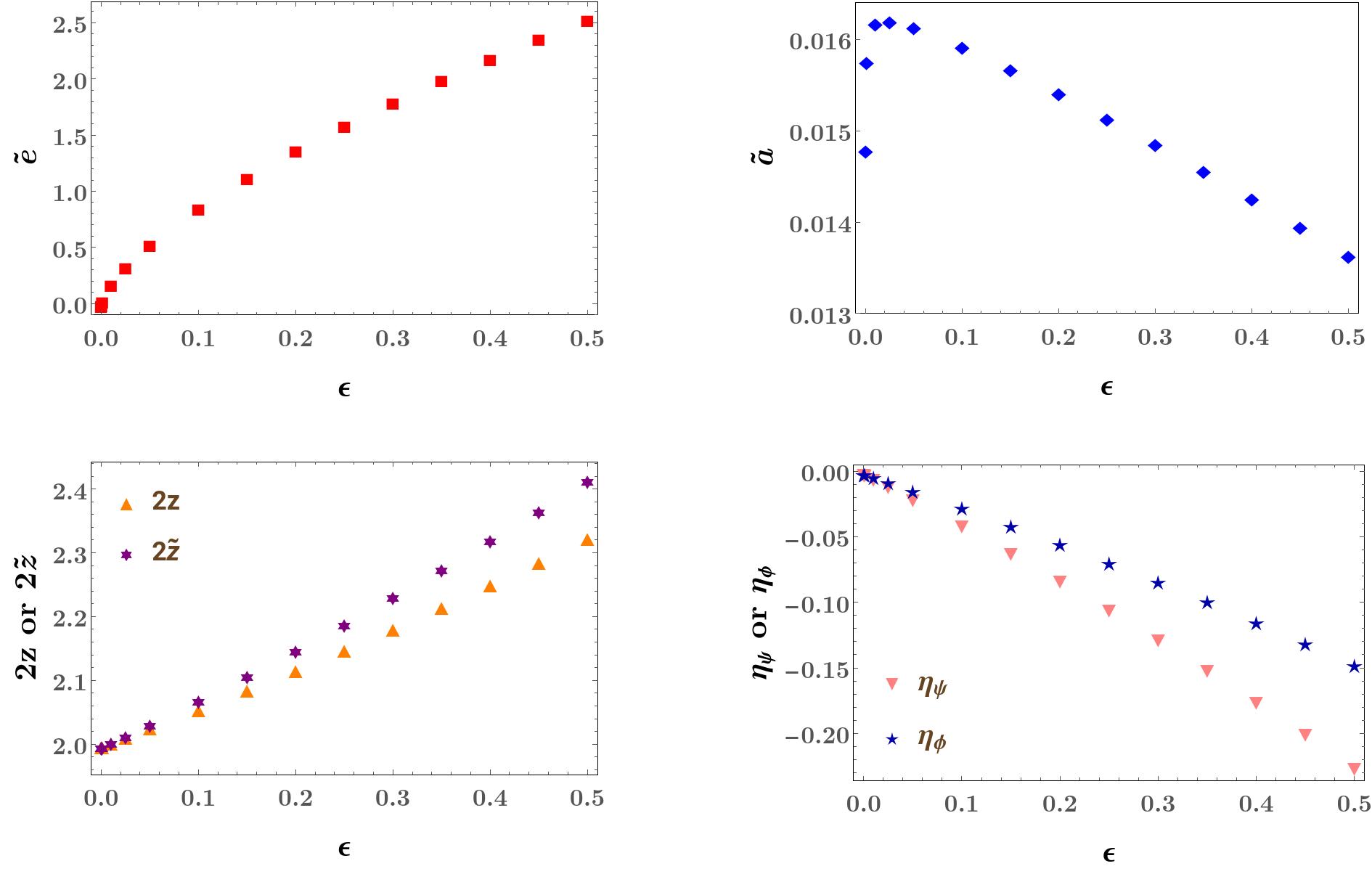
Figure 3: The fixed-point values of $\tilde{e}$, $\tilde{a}$, $2\,z$, $2\,\tilde{z}$, $\eta_{\psi}$, and $\eta_{\phi}$, computed numerically from the zeroes of the two beta functions, plotted as functions of $\epsilon\in(0,1/2]$.

$$\frac{\beta_{a}^{(0)}}{\tilde{e}} =\bigg{[}\tilde{a}^{4}\left\{3\left(3\,\mathcal{U}_{2}-2\,\mathcal{U}_{3}\right)\chi^{2/3}\,{\tilde{e}}^{\frac{1}{2}}-48\,\mathcal{U}_{1}\right\}+2\,\tilde{a}^{3}\left\{3\left(19\,\mathcal{U}_{2}+8\,\mathcal{U}_{3}\right)\chi^{2/3}\,{\tilde{e}}^{\frac{1}{2}}-4\,\mathcal{U}_{1}\left(8\,\mathcal{U}_{2}+\mathcal{U}_{3}\right)\tilde{e}^{3/2}+72\,\mathcal{U}_{1}\right\}$$

$$\qquad+4\,\tilde{a}^{2}\left[4\,\mathcal{U}_{1}\left\{\left(8\,\mathcal{U}_{2}+3\,\mathcal{U}_{3}\right)\tilde{e}^{3/2}-12\right\}-3\,\chi^{2/3}{\tilde{e}}^{\frac{1}{2}}\left\{\mathcal{U}_{2}\left(\left(8\,\mathcal{U}_{2}+5\,\mathcal{U}_{3}\right)\tilde{e}^{3/2}+47\right)+12\,\mathcal{U}_{3}\right\}\right]$$

$$\qquad+24\,\tilde{a}\left[\chi^{2/3}\,{\tilde{e}}^{\frac{1}{2}}\left\{\mathcal{U}_{2}\left(25+2\,\mathcal{U}_{3}\,\tilde{e}^{3/2}\right)+8\,\mathcal{U}_{3}\right\}+\mathcal{U}_{1}\left(4-4\,\,\mathcal{U}_{3}\,\tilde{e}^{3/2}\right)\right]$$

$$\qquad+6\,\mathcal{U}_{1}\,\tilde{a}^{5}+16\,\mathcal{U}_{3}\,{\tilde{e}}^{\frac{1}{2}}\left(9\,\mathcal{U}_{2}\,\chi^{2/3}\,\tilde{e}^{3/2}+4\,\mathcal{U}_{1}\,\tilde{e}-6\,\chi^{2/3}\right)\bigg{]}$$

$$\qquad\times\frac{-\,\chi^{-1}\,\tilde{e}/2}{\tilde{a}^{2}\left(4\,{\mathcal{U}}_{1}\tilde{e}-18\,\chi^{2/3}\right)+2\,\tilde{a}\left(15\,{\mathcal{U}}_{2}\,\chi^{2/3}\,\tilde{e}^{3/2}-8\,{\mathcal{U}}_{1}\tilde{e}+18\,\chi^{2/3}\right)+3\,\chi^{2/3}\,\tilde{a}^{3}+4\left(9\,{\mathcal{U}}_{2}\,\chi^{2/3}\tilde{e}^{3/2}+4\,{\mathcal{U}}_{1}\,\tilde{e}-6\,\chi^{2/3}\right)}\,,$$ (43)

$$\beta_{a}^{(1)} =\frac{3\,\chi^{7/3}\,\tilde{a}\,\tilde{e}^{3/4}\left[\,{\mathcal{U}}_{2}\left(6+\tilde{a}\right)\chi^{-4/3}\,\,\tilde{e}^{3/4}+\frac{2}{3}\,{\mathcal{U}}_{1}\,{\tilde{e}}^{1/4}\,\right]}{-4\,{\mathcal{U}}_{1}\,\chi^{1/3}\,\tilde{a}\,\tilde{e}+6\,{\mathcal{U}}_{2}\left(6+5\,\tilde{a}\right)\tilde{e}^{3/2}+3\,\tilde{a}\left[\,12-\left(6-\tilde{a}\right)\tilde{a}\,\right]+8\left({\mathcal{U}}_{1}\,\chi^{1/3}\,\tilde{e}-3\right)}\,,$$ (44)

where

$$\tilde{e}=e^{4/3}\text{ and }\chi=2-\tilde{a}\,.$$ (45)

Using these expressions, one can easily find the explicit expressions for $z$, $\tilde{z}$, $\eta_{\psi}$, and $\eta_{\phi}$. We do not write those here for the sake of brevity. Since we are interested in the behaviour at the IR energy scales, we determine the RG flows with respect to the floating mass scale $\mu\,e^{-l}$ (i.e., with respect to an increasing logarithmic length scale $l$), which are given by the derivatives

$$\frac{de}{dl}\equiv-\beta_{e}\text{ and }\frac{d\tilde{a}}{dl}\equiv-\beta_{a}\,,$$ (46)

for the two coupling constants $e$ and $\tilde{a}$, respectively.

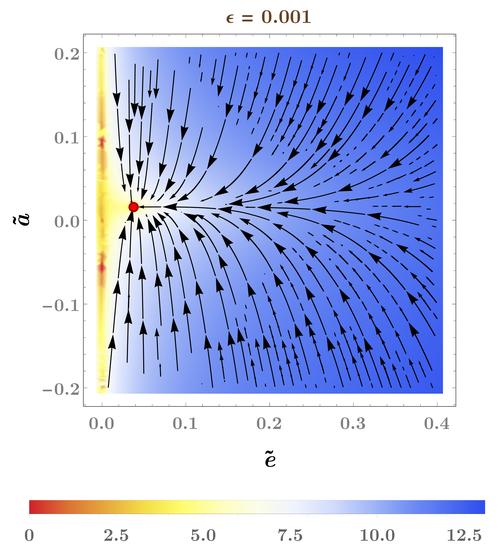
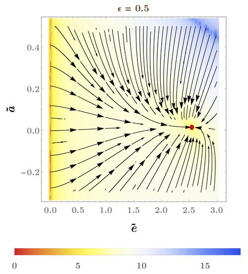
Figure 4: The RG flows in the $\tilde{e}$-$\tilde{a}$ plane for two different values of $\epsilon$: (a) $\epsilon=10^{-3}$ representing the regime around $d=d_{c}$ and (b) $\epsilon=1/2$ representing the regime around $d=2$ (which is the actual/physical dimension of the theory). The red disc represents the IR-stable fixed point in each case. The contour-shading (with the values shown in the plot-legends) corresponds to the natural logarithm of the norm of the flow vector $\{-\beta_{e},\,-\beta_{a}\}$ plus (a) 17 and (b) 19, respectively.

IV.2 Stable fixed points

The fixed points of the theory are obtained as the points where the two beta functions, viz. $\beta_{e}$ and $\beta_{a}$, go to zero simultaneously. The nomenclature originates from the fact that these are are the equilibrium points of the differential equations describing the RG flows in the space of the two coupling constants, $e$ and $\tilde{a}$. Due to the complicated form of the beta functions, it is not feasible to obtain closed-form expressions for these fixed points. Hence, we find their values numerically for a given value of $\epsilon$. In order to determine the stability of a fixed point, one needs to figure out whether the flow lines (in the IR), given by the vector field with the components $\{-\beta_{e},\,-\beta_{a}\}$ in the $\tilde{e}$-$\tilde{a}$ plane, are towards or away from it. Accordingly, they are classified as stable or unstable. The values of the coupling constants, $z$, $\tilde{z}$, $\eta_{\psi}$, and $\eta_{\phi}$ at the stable fixed points, as functions of $\epsilon$, are shown in Fig. 3. In the range $\epsilon\in(0,1/2]$, we find precisely one stable fixed point for each value of $\epsilon$. The stable nature of these fixed points have been illustrated by the RG flows for $\epsilon=10^{-3}$ and $\epsilon=1/2$ in Fig. 4, which is obvious from the fact that the RG flow trajectories converge towards it while flowing from a high value of the floating mass scale to lower and lower values.

An important observation is that the values of $\tilde{z}(\epsilon)$ [cf. Fig. 3] show that we have a flattening of the Fermi surface at the hot-spots after we regularize the theory. This is because the scaling is given by $k_{d-1}^{1/\tilde{z}}\sim k_{d}^{2}\Rightarrow k_{d-1}\sim k_{d}^{2\,\tilde{z}}$. While at tree-level, $2\,\tilde{z}=2$, we find that the interactions drive its value to greater than $2$, as seen from Fig. 3. Furthermore, we would like to point out that both the fermionic and bosonic anomalous dimensions remain negative, unlike the results found in Ref. [67].

V Discussions and outlook

In this paper, we have revisited the QFT of the quantum critical point emerging at the continuous phase transition from a normal metal phase to an ordered phase involving an incommensurate CDW modulation. In our one-loop computations, we have used a dressed boson propagator by including the Landau-damping correction, which is instrumental in inducing the non-Fermi liquid behaviour with a characteristic scaling of $\text{sgn}(k_{0})|k_{0}|^{2/3}$ for the fermion self-energy [19, 20, 21, 52, 53, 54, 73]. In Ref. [67], the authors computed the fermion self-energy $\Sigma(k)$ by assuming the ad hoc form of the boson-self energy $\tilde{\Pi}(q)$ to be $\propto-q_{d-1}$, which they argue is generated in RG due to symmetry arguments. However, a careful analysis shows that RG procedure generates a term proportional to $e_{k}$ and, additionally, terms with Landau damping [cf. Eq. (13)]. As a consequence of not including the all-important Landau-damped term in the dressed bosonic propagator, they do not obtain any contribution in $\Sigma(k)$ proportional to $\mathbf{\Gamma}\cdot\mathbf{K}$ and, hence, miss the crucial $\text{sgn}(k_{0})|k_{0}|^{2/3}$-dependence at $d=2$. They concluded that the correct frequency-dependence would show up at two-loop order. Although Halbinger et al. obtain a part proportional to $\gamma_{d-1}$ in the one-loop fermion self-energy, which leads to a flattening of the Fermi surface at the hot-spots (as found in the RPA calculations of Ref. [66]), that term does not give the correct value of the upper critical dimension $d_{c}$ as $5/2$. This is because this term has a factor $\Gamma(3/2-d)$, which first blows up at $d=3/2$. But of course there are further poles of the Gamma-function for $d=5/2,\,7/2,\cdots$ as well. Consequently, there is a singular contribution showing up at $d=d_{c}$ which contributes to the beta functions. Their integrals are actually somewhat similar to the scenario for our $I_{3}$ calculation [where we retain only the term proportional $\tilde{a}$ in our $\tilde{\Pi}(q)$], which can capture only a subleading scaling behaviour.

While we address the problem with two hot-spots in the incommensurate CDW setting in two dimensions, it will be worthwhile to extend it to the case of three dimensions [74], where we expect a marginal Fermi liquid behaviour, analogous to the results found in Refs. [20, 21, 53]. Another interesting direction to investigate is the scenario when the Fermi surface harbours two pairs of hot-spots [75]. Last, not not the least, we would like to compute the nature of superconducting instabilities in the presence of these critical CDW bosons, utilizing the RG set-ups constructed in Refs. [23, 59].

Appendix: Details of calculating the $b$-dependent part of $\Sigma_{2}$

In this appendix, we compute the $b$-dependent part of the fermion self-energy contribution from $\Sigma_{2}$ [cf. Eqs. (16) and (18)]. Starting with Eq. (24), we define

$$\Sigma_{2}(\mathbf{0},k_{d},k_{d-1}) =e^{2}\,\mu^{x_{e}}\left(I_{4}+I_{5}\right)$$ (47)

where

$$I_{4}=\int_{q,\,e_{q}<0}\frac{\delta_{q-k}}{\mathbf{Q}^{2}+\delta^{2}_{q-k}}\times\frac{1}{q_{d}^{2}+\tilde{a}\,e_{q}+e^{2}\,\mu^{x_{e}}\,b\,|\mathbf{Q}|^{d-1}/\sqrt{|e_{q}|}}\,,$$ (48)

and

$$I_{5}=\int_{q,\,e_{q}>0}\frac{\delta_{q-k}}{\mathbf{Q}^{2}+\delta^{2}_{q-k}}\times\frac{1}{q_{d}^{2}+\tilde{a}\,e_{q}}\,,$$ (49)

where $\delta_{q-k}=e_{q}+e_{-k}+k_{d}^{2}/2+q_{d}^{2}/2-2\,k_{q}\,q_{d}$. However, the part $I_{5}$ is included in $I_{3}$, whose computation has been detailed in the main text itself. Hence, we focus on $I_{4}$ here.

To simply the calculations a bit, we set $k_{d}$ to zero to obtain

$$I_{4} =\int_{q,\,e_{q}>0}\frac{q_{d}^{2}/2-e_{q}-k_{d-1}}{\mathbf{Q}^{2}+\left(q_{d}^{2}/2-e_{q}-k_{d-1}\right)^{2}}\times\frac{1}{q_{d}^{2}-\tilde{a}\,e_{q}+e^{2}\,\mu^{x_{e}}\,b\,|\mathbf{Q}|^{d-1}/\sqrt{e_{q}}}$$

$$=\int_{0}^{\infty}\frac{du}{\sqrt{u/2}}\int_{0}^{\infty}de_{q}\int_{-\infty}^{\infty}\frac{d^{d-1}\mathbf{Q}}{(2\,\pi)^{d+1}}\,\frac{u-e_{q}-k_{d-1}}{|\mathbf{Q}|^{2}+\left(u-e_{q}-k_{d-1}\right)^{2}}\,\frac{1}{2\,u-\tilde{a}\,e_{q}+e^{2}\,\mu^{x_{e}}\,b\,|\mathbf{Q}|^{d-1}/\sqrt{e_{q}}}\quad\left[\text{where }2\,u={q_{d}^{2}}\right]$$ (50)

Observing that the first factor of the integrand forces the dominant contribution to be concentrated around the region $|\mathbf{Q}|\sim 0$ and $u\sim e_{q}+k_{d-1}$. As for the second factor, the dominant contribution comes from $e_{q}\sim|\mathbf{Q}|^{2\,(d-1)/3}$. Hence, we can substitute $u\sim e_{q}+k_{d-1}$ in the $\sqrt{u}$ factor in the overall denominator and the $2\,u$ term in the denominator of the second factor, and extend the lower limit of the integral over $u$ to $-\infty$, leading to

$$I_{4} \simeq\int_{0}^{\infty}\frac{du}{\sqrt{e_{q}+k_{d-1}}}\int_{0}^{\infty}de_{q}\int_{-\infty}^{\infty}\frac{d^{d-1}\mathbf{Q}}{(2\,\pi)^{d+1}}\,\frac{u-e_{q}-k_{d-1}}{|\mathbf{Q}|^{2}+\left(u-e_{q}-k_{d-1}\right)^{2}}\,\frac{\sqrt{2}}{\left(2-\tilde{a}\right)e_{q}+2\,k_{d-1}+e^{2}\,\mu^{x_{e}}\,b\,|\mathbf{Q}|^{d-1}/\sqrt{e_{q}}}$$

$$=0\,.$$ (51)

Hence, to leading order, the $I_{4}$ integral vanishes, and there remains no $b$-dependent term.

References

• Holstein et al. [1973] T. Holstein, R. E. Norton, and P. Pincus, de Haas-van Alphen effect and the specific heat of an electron gas, Phys. Rev. B 8, 2649 (1973).
• Metlitski and Sachdev [2010a] M. A. Metlitski and S. Sachdev, Quantum phase transitions of metals in two spatial dimensions. I. Ising-nematic order, Phys. Rev. B 82, 075127 (2010a).
• Oganesyan et al. [2001] V. Oganesyan, S. A. Kivelson, and E. Fradkin, Quantum theory of a nematic Fermi fluid, Phys. Rev. B 64, 195109 (2001).
• Metzner et al. [2003] W. Metzner, D. Rohe, and S. Andergassen, Soft Fermi surfaces and breakdown of Fermi-liquid behavior, Phys. Rev. Lett. 91, 066402 (2003).
• Dell’Anna and Metzner [2006] L. Dell’Anna and W. Metzner, Fermi surface fluctuations and single electron excitations near Pomeranchuk instability in two dimensions, Phys. Rev. B 73, 045127 (2006).
• Kee et al. [2003] H.-Y. Kee, E. H. Kim, and C.-H. Chung, Signatures of an electronic nematic phase at the isotropic-nematic phase transition, Phys. Rev. B 68, 245109 (2003).
• Lawler et al. [2006] M. J. Lawler, D. G. Barci, V. Fernández, E. Fradkin, and L. Oxman, Nonperturbative behavior of the quantum phase transition to a nematic Fermi fluid, Phys. Rev. B 73, 085101 (2006).
• Rech et al. [2006] J. Rech, C. Pépin, and A. V. Chubukov, Quantum critical behavior in itinerant electron systems: Eliashberg theory and instability of a ferromagnetic quantum critical point, Phys. Rev. B 74, 195126 (2006).
• Wölfle and Rosch [2007] P. Wölfle and A. Rosch, Fermi liquid near a quantum critical point, Journal of Low Temperature Physics 147, 165 (2007).
• Maslov and Chubukov [2010] D. L. Maslov and A. V. Chubukov, Fermi liquid near Pomeranchuk quantum criticality, Phys. Rev. B 81, 045110 (2010).
• Quintanilla and Schofield [2006] J. Quintanilla and A. J. Schofield, Pomeranchuk and topological Fermi surface instabilities from central interactions, Phys. Rev. B 74, 115126 (2006).
• Yamase and Kohno [2000] H. Yamase and H. Kohno, Instability toward formation of quasi-one-dimensional Fermi surface in two-dimensional t-J model, Journal of the Physical Society of Japan 69, 2151 (2000).
• Yamase et al. [2005] H. Yamase, V. Oganesyan, and W. Metzner, Mean-field theory for symmetry-breaking Fermi surface deformations on a square lattice, Phys. Rev. B 72, 035114 (2005).
• Halboth and Metzner [2000] C. J. Halboth and W. Metzner, d-wave superconductivity and Pomeranchuk instability in the two-dimensional Hubbard model, Phys. Rev. Lett. 85, 5162 (2000).
• Jakubczyk et al. [2008] P. Jakubczyk, P. Strack, A. A. Katanin, and W. Metzner, Renormalization group for phases with broken discrete symmetry near quantum critical points, Phys. Rev. B 77, 195120 (2008).
• Zacharias et al. [2009] M. Zacharias, P. Wölfle, and M. Garst, Multiscale quantum criticality: Pomeranchuk instability in isotropic metals, Phys. Rev. B 80, 165116 (2009).
• Kim et al. [2008] E.-A. Kim, M. J. Lawler, P. Oreto, S. Sachdev, E. Fradkin, and S. A. Kivelson, Theory of the nodal nematic quantum phase transition in superconductors, Phys. Rev. B 77, 184514 (2008).
• Huh and Sachdev [2008] Y. Huh and S. Sachdev, Renormalization group theory of nematic ordering in d-wave superconductors, Phys. Rev. B 78, 064512 (2008).
• Dalidovich and Lee [2013] D. Dalidovich and S.-S. Lee, Perturbative non-Fermi liquids from dimensional regularization, Phys. Rev. B 88, 245106 (2013).
• Mandal and Lee [2015] I. Mandal and S.-S. Lee, Ultraviolet/infrared mixing in non-Fermi liquids, Phys. Rev. B 92, 035141 (2015).
• Mandal [2016a] I. Mandal, UV/IR mixing in non-Fermi liquids: higher-loop corrections in different energy ranges, The European Physical Journal B 89, 278 (2016a).
• Eberlein et al. [2016] A. Eberlein, I. Mandal, and S. Sachdev, Hyperscaling violation at the Ising-nematic quantum critical point in two-dimensional metals, Phys. Rev. B 94, 045133 (2016).
• Mandal [2016b] I. Mandal, Superconducting instability in non-Fermi liquids, Phys. Rev. B 94, 115138 (2016b).
• Mandal [2024] I. Mandal, Erratum: Superconducting instability in non-Fermi liquids [Phys. Rev. B 94, 115138 (2016)], Phys. Rev. B 109, 079902 (2024).
• Metlitski and Sachdev [2010b] M. A. Metlitski and S. Sachdev, Quantum phase transitions of metals in two spatial dimensions. II. Spin density wave order, Phys. Rev. B 82, 075128 (2010b).
• Abanov and Chubukov [2004] A. Abanov and A. Chubukov, Anomalous scaling at the quantum critical point in itinerant antiferromagnets, Physical Review Letters 93, 255702 (2004).
• Abanov and Chubukov [2000] A. Abanov and A. V. Chubukov, Spin-Fermion model near the quantum critical point: One-loop renormalization group results, Physical Review Letters 84, 5608 (2000).
• Sur and Lee [2015] S. Sur and S.-S. Lee, Quasilocal strange metal, Phys. Rev. B 91, 125136 (2015).
• Mandal [2017] I. Mandal, Scaling behaviour and superconducting instability in anisotropic non-Fermi liquids, Annals of Physics 376, 89 (2017).
• Schlief et al. [2017] A. Schlief, P. Lunts, and S.-S. Lee, Exact critical exponents for the antiferromagnetic quantum critical metal in two dimensions, Phys. Rev. X 7, 021010 (2017).
• Lunts et al. [2017] P. Lunts, A. Schlief, and S.-S. Lee, Emergence of a control parameter for the antiferromagnetic quantum critical metal, Phys. Rev. B 95, 245109 (2017).
• Baskaran and Anderson [1988] G. Baskaran and P. W. Anderson, Gauge theory of high-temperature superconductors and strongly correlated Fermi systems, Phys. Rev. B 37, 580 (1988).
• Ioffe and Larkin [1989] L. B. Ioffe and A. I. Larkin, Gapless fermions and gauge fields in dielectrics, Phys. Rev. B 39, 8988 (1989).
• Lee [1989] P. A. Lee, Gauge field, Aharonov-Bohm flux, and high-Tc superconductivity, Phys. Rev. Lett. 63, 680 (1989).
• Lee and Nagaosa [1992] P. A. Lee and N. Nagaosa, Gauge theory of the normal state of high-Tc superconductors, Phys. Rev. B 46, 5621 (1992).
• Blok and Monien [1993] B. Blok and H. Monien, Gauge theories of high-Tc superconductors, Phys. Rev. B 47, 3454 (1993).
• Ubbens and Lee [1994] M. U. Ubbens and P. A. Lee, Superconductivity phase diagram in the gauge-field description of the t-J model, Phys. Rev. B 49, 6853 (1994).
• Nayak and Wilczek [1994a] C. Nayak and F. Wilczek, Non-Fermi liquid fixed point in 2 + 1 dimensions, Nuclear Physics B 417, 359 (1994a).
• Chakravarty et al. [1995] S. Chakravarty, R. E. Norton, and O. F. Syljuåsen, Transverse gauge interactions and the vanquished Fermi liquid, Physical Review Letters 74, 1423 (1995).
• Reizer [1989] M. Y. Reizer, Relativistic effects in the electron density of states, specific heat, and the electron spectrum of normal metals, Phys. Rev. B 40, 11571 (1989).
• Halperin et al. [1993] B. I. Halperin, P. A. Lee, and N. Read, Theory of the half-filled Landau level, Phys. Rev. B 47, 7312 (1993).
• Polchinski [1994] J. Polchinski, Low-energy dynamics of the spinon-gauge system, Nuclear Physics B 422, 617 (1994).
• Altshuler et al. [1994] B. L. Altshuler, L. B. Ioffe, and A. J. Millis, Low-energy properties of fermions with singular interactions, Phys. Rev. B 50, 14048 (1994).
• Nayak and Wilczek [1994b] C. Nayak and F. Wilczek, Renormalization group approach to low temperature properties of a non-Fermi liquid metal, Nuclear Physics B 430, 534 (1994b).
• Lee [2009] S.-S. Lee, Low-energy effective theory of Fermi surface coupled with U(1) gauge field in $2+1$ dimensions, Phys. Rev. B 80, 165102 (2009).
• Mross et al. [2010] D. F. Mross, J. McGreevy, H. Liu, and T. Senthil, Controlled expansion for certain non-Fermi-liquid metals, Phys. Rev. B 82, 045121 (2010).
• Jiang et al. [2013] H.-C. Jiang, M. S. Block, R. V. Mishmash, J. R. Garrison, D. N. Sheng, O. I. Motrunich, and M. P. A. Fisher, Non-Fermi-liquid d-wave metal phase of strongly interacting electrons, Nature (London) 493, 39 (2013).
• Chung et al. [2013] S. B. Chung, I. Mandal, S. Raghu, and S. Chakravarty, Higher angular momentum pairing from transverse gauge interactions, Phys. Rev. B 88, 045127 (2013).
• Wang et al. [2014] Z. Wang, I. Mandal, S. B. Chung, and S. Chakravarty, Pairing in half-filled Landau level, Annals of Physics 351, 727 (2014).
• Sur and Lee [2014] S. Sur and S.-S. Lee, Chiral non-Fermi liquids, Phys. Rev. B 90, 045121 (2014).
• Lee [2018] S.-S. Lee, Recent developments in non-Fermi liquid theory, Annual Review of Condensed Matter Physics 9, 227–244 (2018).
• Pimenov et al. [2018] D. Pimenov, I. Mandal, F. Piazza, and M. Punk, Non-Fermi liquid at the FFLO quantum critical point, Phys. Rev. B 98, 024510 (2018).
• Mandal [2020] I. Mandal, Critical Fermi surfaces in generic dimensions arising from transverse gauge field interactions, Phys. Rev. Research 2, 043277 (2020).
• Mandal and Fernandes [2023] I. Mandal and R. M. Fernandes, Valley-polarized nematic order in twisted moiré systems: In-plane orbital magnetism and crossover from non-Fermi liquid to Fermi liquid, Phys. Rev. B 107, 125142 (2023).
• Abrikosov [1974] A. A. Abrikosov, Calculation of critical indices for zero-gap semiconductors, Journal of Experimental and Theoretical Physics 39, 709 (1974).
• Moon et al. [2013] E.-G. Moon, C. Xu, Y. B. Kim, and L. Balents, Non-Fermi-liquid and topological states with strong spin-orbit coupling, Phys. Rev. Lett. 111, 206401 (2013).
• Nandkishore and Parameswaran [2017] R. M. Nandkishore and S. A. Parameswaran, Disorder-driven destruction of a non-Fermi liquid semimetal studied by renormalization group analysis, Phys. Rev. B 95, 205106 (2017).
• Mandal and Nandkishore [2018] I. Mandal and R. M. Nandkishore, Interplay of Coulomb interactions and disorder in three-dimensional quadratic band crossings without time-reversal symmetry and with unequal masses for conduction and valence bands, Phys. Rev. B 97, 125121 (2018).
• Mandal [2018] I. Mandal, Fate of superconductivity in three-dimensional disordered Luttinger semimetals, Annals of Physics 392, 179 (2018).
• Mandal and Freire [2021] I. Mandal and H. Freire, Transport in the non-Fermi liquid phase of isotropic Luttinger semimetals, Phys. Rev. B 103, 195116 (2021).
• Freire and Mandal [2021] H. Freire and I. Mandal, Thermoelectric and thermal properties of the weakly disordered non-Fermi liquid phase of Luttinger semimetals, Physics Letters A 407, 127470 (2021).
• Mandal and Freire [2022] I. Mandal and H. Freire, Raman response and shear viscosity in the non-Fermi liquid phase of Luttinger semimetals, Journal of Physics: Condensed Matter 34, 275604 (2022).
• Roy et al. [2018] B. Roy, M. P. Kennett, K. Yang, and V. Juričić, From birefringent electrons to a marginal or non-Fermi liquid of relativistic spin-$1/2$ fermions: An emergent superuniversality, Phys. Rev. Lett. 121, 157602 (2018).
• Mandal [2021] I. Mandal, Robust marginal Fermi liquid in birefringent semimetals, Physics Letters A 418, 127707 (2021).
• Holder and Metzner [2014] T. Holder and W. Metzner, Non-Fermi-liquid behavior at the onset of incommensurate $2{k}_{F}$ charge- or spin-density wave order in two dimensions, Phys. Rev. B 90, 161106 (2014).
• Sýkora et al. [2018] J. Sýkora, T. Holder, and W. Metzner, Fluctuation effects at the onset of the $2{k}_{F}$ density wave order with one pair of hot spots in two-dimensional metals, Phys. Rev. B 97, 155159 (2018).
• Halbinger et al. [2019] J. Halbinger, D. Pimenov, and M. Punk, Incommensurate $2{k}_{F}$ density wave quantum criticality in two-dimensional metals, Phys. Rev. B 99, 195102 (2019).
• Senthil and Shankar [2009] T. Senthil and R. Shankar, Fermi surfaces in general codimension and a new controlled nontrivial fixed point, Phys. Rev. Lett. 102, 046406 (2009).
• Metlitski et al. [2015] M. A. Metlitski, D. F. Mross, S. Sachdev, and T. Senthil, Cooper pairing in non-Fermi liquids, Phys. Rev. B 91, 115111 (2015).
• ’t Hooft [1973] G. ’t Hooft, Dimensional regularization and the renormalization group, Nuclear Physics B 61, 455 (1973).
• Weinberg [1973] S. Weinberg, New approach to the renormalization group, Phys. Rev. D 8, 3497 (1973).
• Srednicki [2007] M. Srednicki, Quantum field theory (Cambridge University Press, 2007).
• Rao and Piazza [2023] P. Rao and F. Piazza, Non-fermi-liquid behavior from cavity electromagnetic vacuum fluctuations at the superradiant transition, Phys. Rev. Lett. 130, 083603 (2023).
• Schäfer et al. [2017] T. Schäfer, A. A. Katanin, K. Held, and A. Toschi, Interplay of correlations and kohn anomalies in three dimensions: Quantum criticality with a twist, Phys. Rev. Lett. 119, 046402 (2017).
• Sýkora and Metzner [2021] J. Sýkora and W. Metzner, Fluctuation effects at the onset of $2{k}_{F}$ density wave order with two pairs of hot spots in two-dimensional metals, Phys. Rev. B 104, 125123 (2021).