RUBIES: JWST/NIRSpec Confirmation of an Infrared-luminous, Broad-line Little Red Dot with an Ionized Outflow

Abstract

The JWST discovery of “little red dots” (LRDs) is reshaping our picture of the early Universe, yet the physical mechanisms driving their compact size and UV-optical colors remain elusive. Here we report an unusually bright LRD ($z_{\rm spec}=3.1$) observed as part of the RUBIES program. This LRD exhibits broad emission lines (FWHM$\sim 4000\,\rm km\,s^{-1}$), a blue UV continuum, a clear Balmer break and a red continuum sampled out to rest-frame 4 $\mu\mathrm{m}$ with MIRI. We develop a new joint galaxy and active galactic nucleus (AGN) model within the Prospector Bayesian inference framework and perform spectrophotometric modeling using NIRCam, MIRI, and NIRSpec/Prism observations. Our fiducial model reveals a $M_{*}\sim 10^{9}~{}{\rm M}_{\odot}$ galaxy alongside a dust-reddened AGN driving the optical emission. Explaining the rest-frame optical color as a reddened AGN requires $A_{\rm V}\gtrsim 4$, suggesting that a great majority of the accretion disk energy is re-radiated as dust emission. Yet despite clear AGN signatures, we find a surprising lack of hot torus emission, which implies that either the dust emission in this object must be cold, or the red continuum must instead be driven by a massive, evolved stellar population of the host galaxy—seemingly inconsistent with the high EW broad lines (H$\alpha$ rest-frame EW $\sim 800$ Å). The widths and luminosities of Pa-$\beta$, Pa-$\delta$, Pa-$\gamma$, and H$\alpha$ imply a modest black hole mass of $M_{\rm BH}\sim 10^{8}$ M_⊙. Additionally, we identify a narrow blue-shifted He i $\lambda\,1.083\,\mu$m absorption feature in NIRSpec/G395M spectra, signaling an ionized outflow with kinetic energy up to $\sim 1$% the luminosity of the AGN. The low redshift of RUBIES-BLAGN-1 combined with the depth and richness of the JWST imaging and spectroscopic observations provide a unique opportunity to build a physical model for these so-far mysterious LRDs, which may prove to be a crucial phase in the early formation of massive galaxies and their supermassive black holes.

1 Introduction

Observations from the James Webb Space Telescope (JWST) have unveiled an intriguing sample of extremely red sources. As they typically also show a compact morphology these objects have been named “little red dots” (LRDs; Matthee et al. 2023), and they are characterized by a red continuum in the rest-frame optical, a faint blue component in the rest-frame ultraviolet (UV), and often broad Balmer lines indicative of active galactic nuclei (AGNs). Spectroscopic follow-up of LRDs selected based on NIRCam colors has confirmed a surprising ubiquity of broad emission lines, strongly suggesting an AGN component in the rest-frame optical (Greene et al., 2023; Labbé et al., 2023a).

At the same time, interpreting the spectral energy distributions (SEDs) of the LRDs remains difficult. It is still unclear how to model the different spectral components, and which parts of the SED are galaxy or AGN dominated. Common galaxy-only or AGN-only models struggle to simultaneously describe the blue slope in the rest-frame UV, and the very red slope toward the rest-frame optical. Early joint modeling of the two components (e.g., Yang et al. 2020; Furtak et al. 2023a; Williams et al. 2023; Vidal-García et al. 2024) has yielded ambiguous interpretations, while no consensus has been reached about whether the UV can be described by scattered AGN light (e.g., Labbé et al., 2023a), scattered galaxy light (e.g., Killi et al., 2023), or simply unobscured star formation (e.g., Matthee et al., 2023).

The infrared (IR) colors pose additional puzzles: the red slope seen in LRDs strongly suggests high dust attenuation, which, when re-emitted in the IR, results in different spectral shapes depending on the AGN or galaxy nature of the source. AGN are typically associated with the presence of hot dust which will have a steeply rising red continuum at $>2\mu$m (Lacy et al., 2004; Richards et al., 2006; Urrutia et al., 2012), whereas the near-IR stellar bump at rest-frame 1.6 $\mu$m leads to a bluer spectral slope (Laurent et al., 2000; Sawicki, 2002). A stacking analysis of LRD candidates in JADES (Eisenstein et al., 2023) has shown a distinct lack of hot dust, yet no definitive conclusion is drawn regarding whether the flat MIRI color precludes the dominance of AGN in the rest optical, given the available data (Williams et al., 2023). Broader samples selected by requiring both a red rest-optical and blue rest-UV continuum without a compactness criterion seem to be consistent with dusty star-formation (Pérez-González et al., 2024), sparking further debate between the galaxy or AGN origins of LRDs.

So far spectroscopic observations of LRDs have been limited to relatively small samples (Kocevski et al., 2023; Harikane et al., 2023; Matthee et al., 2023; Greene et al., 2023; Furtak et al., 2023b), with the majority of available data restricted to JWST/NIRCam grism and/or JWST/Prism spectroscopy (Greene et al., 2023; Kokorev et al., 2023; Killi et al., 2023). The inferred number densities are quite high, comprising a few percent of the galaxy population at $z>5$ (e.g., Matthee et al., 2023) and $\sim 20\%$ of the broad-line AGNs (e.g., Harikane et al., 2023). One lensed LRD presents a galaxy size limit of $<30$ pc, and a implied black hole to galaxy mass ratio of at least a few percent (Furtak et al., 2023b). Understanding how these massive black holes grew as early as $z=8.5$ (Kokorev et al., 2023) in such compact galaxies remains an intriguing puzzle (e.g., Pacucci & Loeb, 2024; Silk et al., 2024).

The absence of medium to high-resolution spectra to date has meant that emission lines cannot be robustly decomposed, preventing robust measurements of gas kinematics. Accordingly, it is also difficult to characterize potential outflows, which are an integral part of AGN feedback (Zakamska & Greene, 2014; Rupke et al., 2017; Davies et al., 2020; Laha et al., 2021). As a consequence, it is unclear in which phase of supermassive black hole growth LRDs are. Although NIRCam/grism spectroscopy has provided emission line kinematics for a larger sample of LRDs (Matthee et al., 2023), these observations are limited in wavelength coverage, typically yielding one or two emission lines rather than a suite of diagnostics.

In this paper, we present a bright LRD at a spectroscopic redshift of $z_{\rm spec}=3.1034\pm 0.0002$ that is luminous in the IR and has multiple broad emission lines indicative of an AGN. RUBIES-BLAGN-1 is discovered as part of the RUBIES program (JWST-GO-4233; PI de Graaff), for which we obtained high signal-to-noise spectra in both the JWST/NIRSpec low-resolution Prism and the medium-resolution G395M modes, allowing for an in-depth characterization of the physics of this object. Notably, RUBIES-BLAGN-1 is detected in JWST/MIRI F770W and F1800W imaging from PRIMER (JWST-GO-1837; PI Dunlop).

The structure of this paper is as follows. Section 2 provides an overview of the data, including imaging, selection, and spectroscopy. Section 3 details the SED modeling, emission-line decomposition, and photoionization modeling. Section 4 presents the results on the inferred AGN and host galaxy properties, gas kinematics, and mass outflow rate. We conclude in Section 5 with discussion of the key findings.

Where applicable, we adopt the best-fit cosmological parameters from the WMAP 9 yr results: $H_{0}=69.32$ ${\rm km\,s^{-1}\,Mpc^{-1}}$, $\Omega_{M}=0.2865$, and $\Omega_{\Lambda}=0.7135$ (Hinshaw et al., 2013), and a Chabrier initial mass function (Chabrier, 2003). Unless otherwise mentioned, we report the median of the posterior, and 1$\sigma$ error bars are the 16th and 84th percentiles.

2 Data

RUBIES is a spectroscopic survey with JWST/NIRSpec that targets $\sim 4000-5000$ NIRCam-selected sources across the UDS and EGS fields using the micro-shutter array (MSA). Observations are obtained with both the low-resolution Prism/CLEAR and medium-resolution G395M/F290LP modes, providing an unprecedented view of red sources at $z>3$. Unique to RUBIES is its highly complete sampling of the extremes in color-magnitude space. RUBIES-BLAGN-1 was selected with highest priority based on its extreme red color ($\rm F150W-F444W>3.0~{}mag$)—roughly 10 objects in CEERS (Barrufet et al., 2023), and merely 13 objects out of all observed in JADES-GOODS-S (Williams et al., 2023) have such a red color. It is subsequently targeted in two of the three masks observed in January 2024. Full details of the survey design and data reduction will be described in A. de Graaff et al. in prep. This section provides a brief summary of the imaging and spectroscopic data.

2.1 Imaging

Figure 1: Photometric observations of RUBIES-BLAGN-1. (a) Cutouts are shown in selected filter bands, including HST/WCS, JWST/NIRCam, and MIRI detections. A color image, composited from NIRCam/F115W, F277W, and F444W, is included as the last panel. Each panel is 5″ in width. (b) RUBIES-BLAGN-1 is bright in F444W ($\sim$ 22 AB mag) and exhibits an extreme red color with F150W-F444W $\sim$ 3.8 mag. The red objects at higher redshifts are included as pink dots for reference (Labbé et al., 2023a, b). The parent sample, including all sources identified from PRIMER having F444W $<$ 27.5 AB mag, is shown in gray. To facilitate a better comparison to the high-$z$ LRDs, the colors of RUBIES-BLAGN-1 interpolated by shifting the observed spectrum to $z=7$ is plotted as a red plus sign. RUBIES-BLAGN-1 is clearly an outlier in the color space, and possibly can be seen as an analog of the high-$z$ LRDs.

The RUBIES targets in the UDS were selected based on public JWST/NIRCam imaging from the PRIMER survey (JWST-GO-1837; PI Dunlop), which provides NIRCam imaging in 8 bands (F090W, F115W, F150W, F200W, F277W, F356W, F444W and F410M) and MIRI imaging in the F770W and F1800W bands. Archival imaging from the Hubble Space Telescope (HST) is obtained from the CANDELS survey (Grogin et al., 2011; Koekemoer et al., 2011), which adds in 7 more bands in F435W, F606W, F814W, F105W, F125W, F140W, and F160W.

We use the latest version (v7.0) of the publicly available image mosaics from the DAWN JWST Archive (DJA). These images were reduced using grizli (Brammer, 2023a), as also described in Valentino et al. (2023), and have a pixel scale of $0.04\arcsec\,{\rm pix}^{-1}$. We run SourceExtractor (Bertin & Arnouts, 1996) in dual image mode, using an inverse-variance weighted stack of F277W, F356W and F444W band as the detection image. Next, for each NIRCam band we construct a mosaic that is PSF-matched to the F444W image to measure fluxes in circular apertures with a radius of $0.16\arcsec$. We then scale the aperture fluxes to the flux measured through a Kron aperture on a PSF-matched version of the detection image, and to the total flux by dividing by the encircled energy of the Kron aperture on the F444W PSF (A. Weibel et al. in prep).

We use a larger circular aperture of radius $0.35\arcsec$ to measure fluxes from the MIRI images. The MIRI images were reduced in August 2023 (v7.0 on the DJA), prior to the release of new photometric calibrations. Following the JWST documentation, we therefore multiply the measured fluxes with a correction factor based on the updated reference file (jwst_miri_photom_0172); a factor 0.85 and 1.03 for the F770W and F1800W bands, respectively. Finally, we use the empirical PSF models of Libralato et al. (2023) to scale the MIRI aperture fluxes to total fluxes. This is motivated by our analysis that RUBIES-BLAGN-1 is unresolved in the long wavelength images. Specifically, we use pysersic (Pasha & Miller, 2023) to perform Sérsic profile fitting to the source in each long-wavelength image (F277W, F356W, F410M, F444W) shown in Fig 1, using empirical PSF models from Weibel et al. in prep. We find that the source is unresolved in all long-wavelength filters, with a half-light size smaller that a single pixel, $R_{\rm e}<0.25$ kpc. For the remainder of the paper, we conservatively use an upper limit for the half-light radius of 1 pixel (0.3 kpc) for all comparisons involving the half-light radius.

Cutouts for all filters are presented in Figure 1 together with the observed colors of RUBIES-BLAGN-1 and the parent sample, highlighting the extreme color, magnitude, and compactness of the source. For reference, we also put RUBIES-BLAGN-1 on a color-color plot of F277W-F356W vs. F277W-F444W—a criterion used in the literature to select red objects at $z\gtrsim 4$ (Labbé et al., 2023a, b). Clearly RUBIES-BLAGN-1 is an outlier when compared to the parent PRIMER sample. Shifting the spectrum of RUBIES-BLAGN-1 to $z=7$ reveals that its colors are similar to those of the high-$z$ LRDs, suggesting it may be taken as a lower-redshift analog.

In addition, we measure upper limits in Spitzer/MIPS 24 $\mu$m, Herschel/PACS 100, 160 $\mu$m, and Herschel/Spire 250, 350 $\mu$m, from the 3D-Herschel project (K. Whitaker et al. in prep). The imaging data is processed following Whitaker et al. (2014), adopting a forced photometry methodology with the addition of both position and flux priors.

2.2 Spectroscopy

Figure 2: JWST/NIRSpec data of RUBIES-BLAGN-1. (a) The first row displays the 2D Prism spectrum, with the rest-frame wavelength shown along the $x$-axis; the histogram indicates the extracted region. The left panel in the second row shows the 1D spectrum in $F_{\lambda}$ as a function of the observed wavelength. Data and uncertainties are plotted in black and blue, respectively. The beige horizontal line is at $y=0$ to guide the eye. The cutout in the F444W band is shown to the right, with the slitlets overlaid. (b) Same as the above figure set, but for the G395M visits. Only the 2D spectrum of the second visit is included, which has a higher signal-to-noise ratio.

The NIRSpec/MSA low-resolution Prism spectra and the medium-resolution G395M spectra presented in this paper were obtained in two visits between January 16 and 19, 2024. For each visit, RUBIES-BLAGN-1 was observed for 48 min in the Prism/Clear mode and 48 min in the G395M/F290LP mode, using a standard 3-shutter slitlet and 3-point nodding pattern.

The data from the different visits are reduced separately using msaexp (Brammer, 2023b). We process the uncalibrated NIRSpec exposures (uncal.fits) through the Stage 1 steps of the JWST calibration pipeline, inserting an improved mask for “snowball” artifacts between the JumpStep and RampFitStep pipeline procedures using snowblind. Next, a $1/f$ correction is applied, after which individual slits are identified and the 2D unrectified data are flat fielded. The sky background is removed by taking image differences of the 2D flux-calibrated spectra cut out from the exposures taken at three offset positions with the standard “3-Shutter Nod” offsets. The final 2D spectra are created by rebinning the pixels from each background-subtracted 2D cutout from the original detector frame with curved spectral traces onto a rectified grid with orthogonal wavelength and cross-dispersion axes with weighted nearest-neighbor coaddition. The rectified 2D spectra are then optimally extracted to obtain 1D spectra.

The reduced Prism spectrum from visit 1 and G395M spectra from visits 1 and 2 are shown in Figure 2. Due to the source location on the mask, the Prism spectrum from visit 2 falls largely ($\sim 50\%$ of the trace) in the chip gap between the two NIRSpec detectors. We find that the wavelengths of the emission lines in this spectrum differ significantly from the Prism spectrum of visit 1 and also from the two grating spectra (by $\Delta v\sim 2000~{}\rm km\,s^{-1}$), and that the flux is a factor 0.75 lower than measured in the other spectra. This likely reflects calibration issues for sources near the edge of the NIRSpec detectors, and in the remainder of the paper we therefore only use the Prism spectrum from visit 1.

To account for the wavelength-dependent slit losses we rescale the Prism spectrum to the NIRCam photometry by fitting a polynomial correction factor within our SED modeling (§ 3.1.1). We then use the best-fit polynomial for the Prism spectrum to perform a slit loss correction to the G395M data.

3 Spectral modeling

3.1 Spectral Energy Distribution

3.1.1 Basic Set-up

The available JWST and HST photometric data are jointly fitted with the full NIRSpec/Prism spectrum within the Prospector inference framework (Johnson et al., 2021), and the posteriors are sampled using the dynamic nested sampler dynesty (Speagle, 2020). The joint spectrophotometric fit follows the methodology in Wang et al. (2023a). Here we reiterate the common elements for completeness, before detailing the modifications driven by the peculiar nature of RUBIES-BLAGN-1. Fitting the G395M spectrum simultaneously requires special treatment for the different line spread functions (LSFs) and slit losses, and we leave this for future work.

We convolve the model spectra with the NIRSpec/Prism instrumental resolution curve. We note that the instrumental broadening of NIRSpec for a point source has currently not yet been calibrated empirically. Given the compactness of RUBIES-BLAGN-1, we construct a model LSF using msafit (de Graaff et al., 2023) for a point source morphology, which at $4~{}\micron$ is approximately a factor 1.7 narrower than the LSF of a uniformly illuminated slit from the JDox. The resulting resolution from our model is higher, because it accounts for the fact that the spatial extent of the point source in the dispersion direction is narrower than the shutter width. Additionally, to account for the wavelength-dependent slit losses, we fit for a polynomial calibration vector of order 7 after applying a wavelength-independent calibration to scale the normalization of the spectrum to the photometry.

3.1.2 Stellar Populations

To motivate the need for a composite galaxy and AGN model, we start fitting RUBIES-BLAGN-1 with a standard Prospector galaxy-only model. Here, no continuum emission from the AGN accretion disk is included, providing a useful baseline against which we can compare the results from our new composite model.

We adopt the MIST stellar isochrones (Choi et al., 2016; Dotter, 2016) and MILES stellar spectral library (Sánchez-Blázquez et al., 2006) in FSPS (Conroy & Gunn, 2010). The star formation history (SFH) is described by the non-parametric Prospector-$\alpha$ model via mass formed in 7 logarithmically-spaced time bins (Leja et al., 2017), with the first bin width decreased to 13.47 Myr to better accommodate the younger age of the universe at $z>3$ (Wang et al., 2024). A mass function prior and a dynamic SFH($M,z$) prior designed for deep JWST surveys are used as well (Wang et al., 2023b). The normalization and dust optical depth of mid-IR AGNs, as well as dust emission (Draine & Li, 2007) are included. We refer the reader to Wang et al. (2024) for a description of the rest of the parameters describing the stellar populations.

3.1.3 AGN Accretion Disk

The observation of unambiguous broad lines in the spectra of RUBIES-BLAGN-1 motivates the modeling of the accretion disk continuum emission. In brief, we approximate the direct UV/optical emission from an AGN accretion disk as piece-wise power laws following Temple et al. (2021). This model is built from SDSS+UKIDSS+WISE AGN and spans the color-luminosity space probed by these surveys. The resulting spectrum of the accretion disk is similar to the SDSS composite spectrum from Vanden Berk et al. (2001), but mitigates the issue of host galaxy contamination. The normalization of the AGN continuum is a free parameter, parameterized as the ratio of the AGN to stellar flux densities at rest-frame 1500 Å. The power-law slopes are fixed to the best fit values in Temple et al. (2021). Since our wavelength range of interest probes the Rayleigh-Jeans tail of the blackbody emission, we do not expect the slopes to vary significantly across different blackbody temperatures.

As for the dust attenuation, the stellar populations are affected by the diffuse dust, described by a Calzetti et al. (2000) curve with a flexible power-law slope (Noll et al., 2009). A free parameter is assigned to the fraction of the starlight allowed to live outside the dust screen entirely, suggesting that some of the blue stars have blown holes in the dust or otherwise exist outside it. This is similar to the scenarios invoked to describe the blue rest-UV slopes in otherwise very red sub-millimeter galaxies (e.g., Hainline et al. 2011). We assume that the light from the accretion disk experiences the same dust attenuation as the stars, but is additionally reddened by a separate dust attenuation curve modeled as a power law with varying normalization and index. In other words, we take the red continuum of RUBIES-BLAGN-1 as indicative of significant dust presence. The range of the power-law attenuation is set such that the flattest slope is Calzetti-like while the steepest slope approximates that of the Small Magellanic Cloud.

Finally, we include a model component that describes hot dust emission from the AGN torus, which typically starts to be observable beyond rest-frame 2 $\mu$m. We adopt the torus model implemented in FSPS (Conroy et al., 2009; Leja et al., 2018), which is based on a simplified CLUMPY model (Nenkova et al., 2008b) with two free parameters: the normalization and dust optical depth in the mid-IR. In practice, this means that the torus always peaks at the same temperature.

We take the combination of the above AGN accretion disk and torus model and the galaxy model (§ 3.1.2) as the fiducial model of this paper. The relevant parameters are listed in Table 1. However, the unknown nature of LRDs means that other possibilities cannot be ruled out a-priori. We thus additionally fit the data with three alternative models, including fitting with AGN light only, without the new dust component, and fitting the data without the UV continuum. We use these other models to infer the systematic errors in our inferred parameters, and to propose discerning hypotheses for future testing. Details are presented in Appendix A.

Table 1: AGN and Dust Model Parameters and Priors

Parameter	Description	Prior
$f_{\mathrm{AGN_{,}bbb}}$	ratio between the AGN and the host galaxy’s flux densities at rest-frame 1500 Å, pre-attentuation	log uniform: $\mathrm{min}=10^{-5}$, $\mathrm{max}=500$
$f_{\mathrm{AGN,torus}}$	ratio between the AGN luminosity in the mid-IR and the host galaxy’s bolometric luminosity	log uniform: $\mathrm{min}=10^{-5}$, $\mathrm{max}=3$
$\tau_{\mathrm{AGN,torus}}$	optical depth of AGN torus dust	log uniform: $\mathrm{min}=5$, $\mathrm{max}=150$
$n_{\mathrm{dust,2}}$	power law index for a Calzetti et al. (2000) attenuation curve	uniform: $\mathrm{min}=-1.0$, $\mathrm{max}=0.4$
$\hat{\tau}_{\rm dust,2}$	optical depth of diffuse dust seen by both the host galaxy and the AGN	uniform: $\mathrm{min}=0$, $\mathrm{max}=4$
$n_{\mathrm{dust,4}}$	power law index for the AGN-only attenuation curve	uniform: $\mathrm{min}=-1.0$, $\mathrm{max}=0.4$
$\hat{\tau}_{\rm dust,4}$	optical depth of dust seen only by the AGN	uniform: $\mathrm{min}=0$, $\mathrm{max}=4$
$f_{\rm nodust}$	fraction of starlight that is not attenuated by the diffuse dust	uniform: $\mathrm{min}=0$, $\mathrm{max}=1$

Note. — The remaining Prospector parameters and priors adopted for the stellar population inference are described in Wang et al. (2024).

3.1.4 AGN Torus

In the above fiducial model, the accretion disk and the torus emissions are independent of each other, meaning that energy balance is not enforced. In other words, the fiducial model does not force the absorbed AGN energy in the rest-UV and optical to be re-emitted into the IR (though energy balance is enforced for the stellar light). This choice is made in light of the concern that the assumption of the attenuated luminosity equaling the emitted luminosity in the IR does not hold in the presence of an angular dependence of dust emission and absorption. Dust emission in a complicated AGN dust torus geometry may have significant inclination dependence, which cannot be modeled with a single unresolved object (e.g., Nenkova et al. 2008a, b. However, given the existing IR upper limits, we find it valuable to calculate the energy balance. We thus consider two variations on the fiducial model.

First, we ignore the IR limits, and let the total AGN luminosity absorbed by dust in the fiducial model to be re-emitted in the IR. In other words, we scale our simplified CLUMPY torus model spectrum by the luminosity absorbed by the dust. The resulting torus emission is then compared to the IR photometric observations.

Second, we perform the test more broadly on the full CLUMPY model (Nenkova et al., 2008b). As mentioned earlier, the torus model as implemented in Prospector is a simplified version. A wide range of factors can affect the resulting SED of the dust emission; accordingly the CLUMPY model has 6 parameters producing a wide range of observed SED shapes, and other models have a different physical picture entirely with their own associated SED shapes (Dullemond & van Bemmel, 2005; Hönig et al., 2006). A detailed characterization of the torus model is out of the scope of this paper. We conduct a simple experiment by randomly drawing CLUMPY models and scaling them to match the total AGN luminosity attenuated by dust. This test allows more freedom in interpreting the IR limits, including in particular extending the range of temperatures in the dust to colder values and allowing variation in the viewing angle.

3.1.5 Emission line Marginalization

In the Prospector fit nebular and AGN emission lines are not interpreted using a physical model, but instead described by simple Gaussians using the methodology in Johnson et al. (2021). However, the standard method of using a single Gaussian is insufficient for our case, given the clear broad-line component visible in the observed spectra (Figure 2). We thus implement a two-component Gaussian model for most lines, consisting of a narrow and a broad component. We also treat the velocities of the hydrogen lines separately from the metal lines, given the expectation that their line widths can differ from the other lines. This is mostly to ensure sufficient flexibility to accurately describe the lines. A total of four parameters are used to fit the emission lines, i.e., separate velocities for hydrogen lines compared to other lines with a broad and narrow component for each type.

The potential non-Gaussianity of the lines, some of which is visible in Figure 2, is not accounted for. In order to avoid the likelihood being skewed by the residuals from the non-Gaussian line kinematics, we impose a 10% error floor in the spectroscopic data, higher than the 5% error floor usually applied for photometry. We also include a multiplicative noise inflation term as a free parameter, with a prior range from 0.5 to 5, serving as both a pressure valve in the event of significant model mismatch and as an additional check on the quality of the fit.

3.2 Emission line Decomposition

Separate from the fitting with Prospector, we perform kinematic modeling of the brightest broad lines to measure the widths and luminosities of the broad and narrow line components. This separate fit is done to have more fine-tuned understanding of the line kinematics outside of the nested sampling fit. We use the medium-resolution spectra covering $2.9-5.1~{}\micron$ to measure the properties of the Pa-$\delta$, Pa-$\gamma$ and He i lines, and fit this complex simultaneously to account for blended lines.

We model each emission line with a broad and narrow Gaussian line profile, and allow for a velocity offset between the two components. We assume uniform priors for the redshift, line fluxes, and velocity dispersions ($\rm\sigma_{\rm broad}\in[700,5000]~{}\rm km\,s^{-1}$; $\rm\sigma_{\rm narrow}\in[0,700]~{}\rm km\,s^{-1}$). The local continuum is modeled as a 2nd-order polynomial. In addition to this emission model, we find a strong absorption feature at $\approx 4.2~{}\micron$ present in both medium-resolution spectra. This is clearly visible in Figure 2, and a zoom-in is shown in Figure 6. We model this feature as a blue-shifted outflow in the He i 10830 Åline, and assume a Gaussian line profile with uniform priors for the flux, velocity dispersion ($\rm\sigma_{\rm outflow}\in[0,1000]~{}\rm km\,s^{-1}$) and velocity offset with respect to the narrow He i component $\Delta v\in[0,2000]~{}\rm km\,s^{-1}$.

As mentioned in Section 3.1.1, we use a model LSF for a point source morphology (de Graaff et al., 2023). Although the model LSF has a systematic uncertainty of $\sim 10-20\%$, we find in Section 4.4 that the narrow line component is substantially broader than the LSF, and is therefore unaffected. Furthermore, to robustly fit the narrow lines in our data we need to account for the under-sampling of the LSF ($\rm FWHM_{LSF}\sim 1~{}pix$) and narrow emission lines. To do so, we construct our model on a wavelength grid that is over-sampled by a factor 5. After convolution with the LSF, the model is integrated and sampled at the original pixel resolution.

We leverage the data from the two independent visits for a better sampling of the LSF. Instead of combining the two spectra, which may introduce further correlated noise, we simultaneously fit to the two spectra. We use the Markov Chain Monte Carlo ensemble sampling method implemented in emcee (Foreman-Mackey et al., 2013) to estimate the posterior distributions of the model parameters.

In addition to our modeling of the medium-resolution data, we also model the low-resolution Prism data, as we find that both the H$\alpha$ and Pa-$\beta$ lines are significantly broader than the Prism LSF. Due to significant issues in the wavelength and flux calibration in the prism spectrum from the 2nd visit, we only use the data from the first visit (i.e., consistent with the Prospector modeling). We fit the two lines individually, following a similar approach as for the medium-resolution data, but with some small modifications.

The observed wavelength of Pa-$\beta$ falls on the edge of the spectrum, and the line is therefore partially cut off. With the added complication of the severe under-sampling of the LSF and uncertainty in the LSF, we adjust our model in two ways: (i) we assume that there is no velocity offset between the broad and narrow line, and (ii) we multiply the instrument broadening ($\rm\sigma_{LSF}$) by a nuisance parameter $f_{\rm LSF}$ to account explicitly for the uncertainty in the LSF. We assume a truncated Gaussian prior for the latter, with $f_{\rm LSF}\in[0.8,1.5]$, a mean of $\mu(f_{\rm LSF})=1.1$ and dispersion $\sigma(f_{\rm LSF})=0.2$ (see Appendix A of de Graaff et al., 2023).

To fit the H$\alpha$ line we additionally include the [N ii]_6549,6585 doublet in the model. We assume that the [N ii] lines are narrow and equal to the narrow line width of H$\alpha$, and fix the flux ratio of the doublet to 1:2.94. Because the narrow line width is a factor $>4$ narrower than the LSF, we cannot constrain the width from the prism data alone. We therefore assume a Gaussian prior for the velocity dispersion of the narrow line based on the estimates from the well-resolved Paschen lines: $\mu(\rm\sigma_{narrow})=250~{}\rm km\,s^{-1}$ and $\sigma(\rm\sigma_{narrow})=50~{}\rm km\,s^{-1}$.

3.3 Single-epoch Black Hole Mass

Reverberation mapping can obtain the radius of the broad-line region from the lag between the variability in the AGN continuum and the corresponding variability in the broad permitted lines (e.g., Blandford & McKee 1982). Empirical correlations have since been derived between the radius and line luminosities and widths in the local universe (e.g., Kaspi et al. 2000; Landt et al. 2013). These relationships allow for the black hole mass to be estimated from single-epoch measurements.

Given the wavelength coverage of RUBIES-BLAGN-1, we estimate the black hole mass via three different scaling relations using the Balmer and Paschen series. Comparing these (mostly) independent estimators helps to mitigate the systematic uncertainties introduced by the application of these methods at higher redshifts and in different physical conditions than where they are calibrated. All line luminosities here are dereddened using the dust attenuation inferred from SED fitting. First, we use the H$\alpha$ scaling relation from Greene & Ho (2005):

$$M_{\rm BH}/M_{\odot}=2.0\cdot 10^{6}~{}\cdot\\ \left(\frac{L_{{\rm H\alpha}}}{10^{42}~{}{\rm erg~{}s^{-1}}}\right)^{0.55}\left(\frac{{\rm FWHM_{H\alpha}}}{10^{3}~{}{\rm km~{}s^{-1}}}\right)^{2.06},$$ (1)

which has an intrinsic systematic scatter of a factor of $\sim 2$.

Second, we adapt the Pa-$\beta$ scaling relation from Kim et al. (2015):

$$M_{\rm BH}/M_{\odot}=10^{7.04}~{}\cdot\\ \left(\frac{L_{\rm Pa-\beta}}{10^{42}~{}{\rm erg~{}s^{-1}}}\right)^{0.48}\left(\frac{{\rm FWHM_{\rm Pa-\beta}}}{10^{3}~{}{\rm km~{}s^{-1}}}\right)^{2},$$ (2)

which has a lower intrinsic scatter of a factor of $\sim 0.2$ dex, but is inferred from a smaller reverberation mapping sample (Kim et al., 2010).

Third, we consider the scaling relation between rest-IR Paschen-series lines and the rest-IR continuum (Landt et al., 2013):

$$\log M_{\rm BH}=0.88~{}\cdot\\ \left(2\log\frac{{\rm FWHM_{\rm H}}}{{\rm km~{}s^{-1}}}+0.5\log\frac{\nu L_{\nu,\rm 1\mu m}}{{\rm erg~{}s^{-1}}}\right)-17.39.$$ (3)

Although this relation has a high intrinsic scatter of $\approx 1\,$dex, it allows us to utilize the better determined Pa-$\delta$ and Pa-$\gamma$ lines, and serves as a consistency check.

In addition, we estimate the AGN bolometric luminosity in two ways to facilitate a comparison to the Eddington limit. First, we apply a standard bolometric correction factor of 10 to the dust-corrected luminosity at rest 5100 Å (e.g., Richards et al. 2006; Shen et al. 2020), and quote this value as our fiducial bolometric luminosity. While imperfect, this model-dependent value represents our best guess for the intrinsic luminosity of the AGN in the context of our preferred AGN model. Second, we base our estimate on the inferred model spectra. We integrate over the observed spectrum with the galaxy contribution subtracted, and then add in the luminosity attenuated by dust. The latter is approximated as the inferred pre-attenuation AGN luminosity, minus the post-attenuation AGN luminosity, based on the dust content from SED fitting. This approximation is likely to be an underestimation, due to the unobserved peak (“big blue bump”; Sanders et al. 1989).

3.4 Photoionization Modeling

We estimate the hydrogen column density associated with the He i absorber by running photoionization models using the C23 version of cloudy (Chatzikos et al., 2023). We adopt the standard AGN radiation field which is a modified version of the Mathews & Ferland (1987) SED with a sub-millimeter break at 10 microns. We calculate a two-dimensional grid of models with hydrogen number density varied in the range 2 $<\log(n_{\textrm{H}})$[cm^-3] $<$ 10 in 0.5 dex steps and ionization parameter varied in the range $-4.5<\log(U)<$ 0 in 0.3 dex steps. The elemental abundances are fixed to solar. The models are run until they reach a hydrogen column density of $\log N_{\textrm{H}}$[cm^-2] = 24.

For each model, we compute $N_{\rm H}$ and $N_{\rm He}(2^{3}S)$ as a function of radius. We use 1D interpolation to find the radius where the predicted $N_{\rm He}(2^{3}S)$ most closely matches the measured value, and record the corresponding $N_{\rm H}$ at that radius. Models that do not reach the observed $N_{\rm He}(2^{3}S)$ are excluded from further analysis.

4 Results

Several previous studies have attempted to disentangle the AGN or galaxy origin of LRDs. Barro et al. (2023) and Kocevski et al. (2023) suggested that the red continuum can be explained by either a heavily obscured quasar or a dusty starburst galaxy, whereas Labbé et al. (2023a) used ALMA non-detections to infer that the compact red sources are not typical dusty star-forming galaxies. The flat MIRI colors have further led to attempts to model the continuum as a reddened but old stellar population (Williams et al., 2023).

With those ideas in mind, we begin by presenting results from fitting only starlight to the rest UV/optical continuum of RUBIES-BLAGN-1 (§4.1). This model serves as a useful benchmark, against which we evaluate our AGN and galaxy composite model (§4.2). Finally, we explore the family of models that are consistent with the mid-to-far infrared data and limits, particularly in the context of dusty torus models that characterize typical AGNs (§4.3). Parameter constraints, including inferred properties of the host galaxy and the AGN are listed in Table 2, and line fluxes and kinematics are listed in Table 3.

Table 2: Inferred Properties of the Host Galaxy and the AGN, and Ancillary Parameters

	Basic measurement
RA [deg]	34.244201
Dec [deg]	-5.245872
$z_{\rm spec}$	3.1034 $\pm$ 0.0002
F150W [AB mag]	25.7$\pm$0.05
F277W [AB mag]	22.3$\pm$0.05
F356W [AB mag]	22.3$\pm$0.05
F444W [AB mag]	21.5$\pm$0.01
F1800W [AB mag]	21.1$\pm$0.05
	Model-inferred property
log $M_{*}/{\rm M}_{\odot}$	$9.25^{+0.15}_{-0.11}$
Age [Gyr]	$0.34^{+0.32}_{-0.14}$
SFR [${\rm M}_{\odot}\,{\rm yr}^{-1}$]	$5.97^{+1.98}_{-4.28}$
log sSFR [${\rm yr}^{-1}$]	$-8.71_{-0.97}^{+0.16}$
log $Z_{*}/{\rm Z}_{\odot}$	$-1.29^{+0.56}_{-0.38}$
$\hat{\tau}_{\rm dust,2}$	$0.42^{+0.09}_{-0.07}$
$n_{\rm dust,2}$	$-0.61^{+0.22}_{-0.16}$
$f_{\rm nodust}$	$0.14^{+0.10}_{-0.04}$
$f_{\rm AGN,7500A}$	$11.69^{+3.01}_{-3.87}$
$f_{\rm AGN,torus}$	$0.08^{+0.79}_{-0.07}$
$\hat{\tau}_{\rm torus}$	$14.08^{+12.19}_{-5.97}$
$\hat{\tau}_{\rm dust,4}$	$3.56^{+0.10}_{-0.11}$
$n_{\rm dust,4}$	$-1.21^{+0.06}_{-0.07}$
	Additional inferred property
$\log M_{\rm BH}/{\rm M}_{\odot}$ , H$\alpha$	8.6 (8.5)
$\log M_{\rm BH}/{\rm M}_{\odot}$ , Pa$\beta$	8.4 (8.3)
$\log M_{\rm BH}/{\rm M}_{\odot}$ , Pa$\delta$	7.9 (7.8)
$\log M_{\rm BH}/{\rm M}_{\odot}$ , Pa$\gamma$	7.9 (7.8)
Bolometric luminosity [${\rm L}_{\odot}$]	$32\times 10^{12}$ ($5\times 10^{12}$)
Eddington luminosity [${\rm L}_{\odot}$]	$(2-13)\times 10^{12}$

4.1 Galaxy-only Best Fit

Figure 3: Spectrophotometric modeling with starlight only. The photometric and spectroscopic data are shown in black, whereas the uncertainty in the observed spectrum is shown in gray. The best-fit model spectrum, which includes the marginalized emission lines) is plotted in orange, whereas the unconvolved galaxy model spectrum is over-plotted in blue. The $x$-axis transits from a linear to a log scale at 5.4 $\mu$m, indicated by the black vertical line, to show the MIRI detections. The spectral regions that are masked due to low S/N, blended, and incomplete lines are shaded in gray. The emission lines included in the marginalization are annotated. $\chi$ is included in the bottom.

As seen from Figure 3, the galaxy-only model produces a good fit in the rest-frame UV-optical and an inferred star mass of $\sim 10^{11}~{}{\rm M}_{\odot}$ with an sSFR of $\sim 10^{-10}~{}{\rm yr^{-1}}$. The rest of the inferred properties are listed in Appendix A, including its mass-weighted age of $\sim 0.8$ Gyr and $A_{\rm V}$ of $\sim 3$.

It would be unusual but not impossible to have such an old massive galaxy (e.g., the quiescent galaxy at $z_{\rm spec}=3.97$, which has $A_{\rm V}\sim 1.4$ in the center; Setton et al. 2024). It would also be surprising to have such strong broad-line features (H$\alpha$ rest-frame EW $\sim 800$ Å) and such a massive black hole with very little continuum contribution from the accretion disk, although AGN broad lines may still exist in older galaxies (Carnall et al., 2023). Moreover, the small size of RUBIES-BLAGN-1 ($<0.3$ kpc, conservatively using an upper limit to half-light radius of $<1$ pixel; see Section 2) implies a very high stellar density (Baggen et al., 2023). This size would alao make RUBIES-BLAGN-1 a small galaxy relative to its peers, but not an outlier among known old galaxies at similar mass and redshift (Wright et al., 2023; Ji et al., 2024). However, the inferred narrow line widths of the Pa-$\gamma$ and Pa-$\delta$ lines ($\sim 250\,\rm km\,s^{-1}$) and small size imply a dynamical mass ${\rm M_{dyn}}\sim 5\,R_{\rm e}\sigma^{2}/G\sim 10^{10}\,{\rm M}_{\odot}$ (where $G$ is the gravitational constant; see e.g., Cappellari et al., 2006), which would be difficult to reconcile with a stellar mass estimate of $10^{11}\,{\rm M}_{\odot}$ even when considering projection effects that may underestimate the true velocity dispersion of the system. We therefore favor the fiducial galaxy and AGN joint fit presented in the following section, but cannot definitively rule out a galaxy-dominated continuum. Follow-up deep medium-resolution data to reveal possible stellar absorption lines, or deeper rest-frame $>30~{}\mu$m data, will help to discriminate the different scenarios.

4.2 UV/Optical Best Fit

Figure 4: Spectrophotometric modeling with the fiducial AGN and host galaxy composite model. (a) Data and best-fits are shown in the same manner as Figure 3. (b) The various components of the model spectrum are illustrated here. Without assuming energy balance, the model predicts the accretion disk emission dominating the spectrum at $\gtrsim 2~{}\mu$m in the observed frame, with little contribution from the torus. (c) Same model, but letting the attenuated AGN luminosity in the UV/optical to be re-emitted in the IR. The resulting torus emission violates the MIRI detection and the upper limit from Spitzer/MIPS. The black vertical line indicates where the NIRSpec/Prism coverage ends.

In Figure 4 we show our fiducial galaxy and AGN joint model. An immediate observation is the capability of our fiducial model to generate a very red slope in the rest optical region and a blue slope in the rest near-UV, providing an effective fit to the observed data. This v-shape in $F_{\lambda}$ is difficult to reproduce with a simple AGN-only model (see Appendix A). As depicted in Figure 4, starlight makes up the rest-UV, whereas the light from the reddened AGN accretion disk dominates the spectrum red-ward of rest 4000 Å.

The model AGN continuum emission is very bright and red due to the large implied dust attenuation and dominates over the wavelength range probed by JWST/MIRI. The torus contributes little to the total light in this fiducial fit even at rest-frame 5 $\mu$m.

The host galaxy has a stellar mass of $\sim 10^{9}~{}{\rm M}_{\odot}$, and a mass-weighted age of $\sim 0.3$ Gyr ($\sim 15$% of the age of the universe). It is metal-poor ($\sim 0.05~{}{\rm Z}_{\odot}$), and slightly below the star-forming main sequence when comparing its sSFR of $\sim 10^{-8.7}~{}{\rm M}_{\odot}\,{\rm yr}^{-1}$ to the value of $\rm sSFR(M_{*}\sim 10^{9}~{}{\rm M}_{\odot})\sim 10^{-8.3}~{}{\rm M}_{\odot}\,{\rm yr}^{-1}$ as reported in Speagle et al. (2014). The dust attenuation is $A_{\rm V}\sim 0.5$, with $\sim 10$% of the total stars outside the dust screen. The inferred star-formation history resembles that of a post-starburst galaxy, likely driven by the presence of a Balmer break.

The preference for a metal-poor solution is primarily caused by the need to predict the UV excess, since the fiducial model essentially couples the UV light to the galaxy. A natural question is thus whether the host galaxy properties are heavily influenced by the UV continuum. We address this question by fitting our fiducial model to the rest optical part of the spectrum only in Appendix A. In brief, we find that the inferred stellar mass as well as the inferred star-formation history in this case are similar to those from the fiducial model, suggesting that the UV continuum is not driving the inferred star formation history or mass.

4.3 IR Constraints and an Inability to Model the Mid-IR with a Standard Hot Torus

Figure 5: Modeling the IR with the CLUMPY torus model (Nenkova et al., 2008b). The JWST photometric data are shown as gray dots, whereas the upper limits from Spitzer/MIPS and Herschel are shown as gray and black triangles, respectively. The curves show random draws that are consistent with the IR upper limits.

While our fiducial model does a fine job fitting the rest-frame UV and optical constraints, the MIRI data are surprisingly flat compared to our expectations for a hot dust component from the torus (Bosman et al., 2023). Thus, we consider the alternative modeling assumptions as listed in Section 3.1.4, where we attempt to self-consistently model the reddened AGN disk emission and the re-emitted torus dust. The AGN torus spectrum from our fiducial Prospector model, re-scaled with the total energy absorbed by dust, is shown in Figure 4 (c). While the model spectrum is marginally consistent with the Herschel upper limits, the MIRI/F1800W and MIPS points are at least a factor of 20 below the predictions from the scaled torus model.

The inability of simple hot AGN torus dust models to explain the observations motivates a more full exploration of the CLUMPY model set (Nenkova et al., 2008b). We draw random models that obey our mid-to-far IR upper limits when scaled by the total energy absorbed by dust, and show 100 examples in Figure 5. This shows that additional freedom in torus clump size, torus shape, and angular dependence of the dust emission and absorption can produce colder AGN dust models which are consistent with the observational constraints. These lower temperatures can be caused by thicker dust shielding which produces a wider and overall colder range of dust temperatures. There is a known population of hot-dust-deficient AGNs which offers further support for this scenario (Hao et al., 2010; Jiang et al., 2010; Mor & Trakhtenbrot, 2011; Lyu et al., 2017).

We note that since the AGN bolometric luminosity from $L_{5100}$ may be $\sim 6-7$ times higher than that inferred from the continuum model, we perform an additional test where we increase the remitted IR luminosity by a factor of 2. In this case, the full CLUMPY model struggles to produce a torus spectrum that is consistent with the IR limits, just making the challenge to model the torus more accute.

Three physical scenarios can be invoked to explain the apparent lack of torus emission. First, the dust emission from LRDs may be in a relatively unexplored regime, being colder than any model in the CLUMPY database. Second, a majority of the energy originated from the big blue bump escapes through some combination of anisotropic dust attenuation or hard X-ray photons and so is not absorbed by dust. Third, the UV part of the accretion disk could be suppressed in a super-Eddington flow (e.g., Abramowicz et al., 1988; Kubota & Done, 2019). Deeper rest-frame mid/far-IR constraints would help to reveal the nature of the source.

4.4 Gas Kinematics

Figure 6: Kinematic emission line decomposition. On the left, we show the emission line fits to the Prism spectrum for the blended H$\alpha$ and [N ii] complex (top) and Pa-$\beta$ line (bottom). Although the narrow line widths are poorly constrained due to the broad LSF (and the partial coverage of Pa-$\beta$), the broad lines are well constrained. On the right, we show the results of our fitting for the Pa-$\delta$ and blended He i and Pa-$\gamma$ lines in the the G395M spectra (top). We find a strong blue-shifted absorption feature in the He i line in the two independent G395M spectra, which we interpret as an ionized outflow. The bottom right shows the observed spectrum divided by the best-fit model emission spectrum. The red shaded region indicates the area used to integrate the optical depth and compute the column density of the absorbing gas. The absorption feature at $4.2~{}\micron$ is present in only one of two visits and corresponds to a detector artefact (see Figure 2).

Table 3: Results of the emission line decomposition

Emission	Flux (total)	Flux (narrow)	$\sigma$ (narrow)	Flux (broad)	$\sigma$ (broad)	EW (total)
	$\rm 10^{-18}~{}erg~{}s^{-1}~{}cm^{-2}$	$\rm 10^{-18}~{}erg~{}s^{-1}~{}cm^{-2}$	km s-1	$\rm 10^{-18}~{}erg~{}s^{-1}~{}cm^{-2}$	km s-1	rest-frame Å
H$\alpha$	$392^{+15}_{-15}$	$109_{-18}^{+22}$	$253_{-51}^{+50}$	$282_{-20}^{+18}$	$2228_{-63}^{+67}$	$832\pm 33$
[N ii]	$67^{+15}_{-15}$					$143\pm 33$
Pa-$\beta$	$103^{+5}_{-4}$	$26^{+5}_{-4}$	$424_{-79}^{+72}$	$77_{-6}^{+5}$	$1929_{-141}^{+149}$	$35\pm 2$
Pa-$\delta$	$31.2^{+1.2}_{-1.2}$	$4.4_{-0.7}^{+1.0}$	$273_{-45}^{+62}$	$26.6^{+1.1}_{-1.1}$	$1700_{-95}^{+114}$	$99\pm 4$
Pa-$\gamma$	$65^{+3}_{-3}$	$6.4^{+0.7}_{-0.7}$	$196_{-26}^{+31}$	$59^{+3}_{-3}$	$1644_{-61}^{+68}$	$217\pm 10$
He i	$59_{-4}^{+5}$	$25_{-3}^{+4}$	$341_{-29}^{+28}$	$34^{+3}_{-3}$	$1327^{+64}_{-64}$	$192^{+17}_{-14}$
Absorption	Outflow flux	${\rm d}v_{\rm outflow}$	$\sigma_{\rm outflow}$			EW
	$\rm 10^{-18}~{}erg~{}s^{-1}~{}cm^{-2}$	km s-1	km s-1			rest-frame Å
He i	$-25_{-4}^{+3}$	$-863_{-113}^{+121}$	$242^{+10}_{-10}$			$-82^{+10}_{-14}$

We show the decomposition into narrow and broad components (§ 3.2) in the Paschen and H$\alpha$ lines in Figure 6, and list the fluxes and velocity dispersions in Table 3. We find that the narrow and broad line widths of the Pa-$\gamma$ and Pa-$\delta$ lines are in good agreement, and that the narrow line flux comprises 14% and 10% of the total line flux, respectively. The narrow and broad line widths of the Pa-$\beta$ emission are broader than the other Paschen lines by approximately $2\sigma$, and with a higher narrow-to-total flux ratio (25%). Although some physical differences may be expected if the different line transitions trace gas in different parts of the broad line region (BLR), the Pa-$\beta$ line is at the very edge of the spectrum which may bias the kinematic fitting. The H$\alpha$ broad line is significantly broader, by a factor $\approx 1.3$, than the Paschen broad lines; the narrow line flux is approximately 30% of the total H$\alpha$ line flux. This may imply that the H$\alpha$ line traces a closer-in region of the BLR compared to the Paschen lines (see e.g. Kim et al., 2010). However, as the narrow H$\alpha$ line and the [N ii] lines are unresolved at the resolution of the Prism, the kinematic fit depends on the model assumptions made (at the $\approx 10\%$ level for the broad line width). Follow-up spectroscopy at higher resolution will be crucial to perform more careful modeling of the H$\alpha$ and [N ii] emission line complex and robustly constrain the narrow-to-total line flux ratio, and to confirm the difference in the broad line width between the Balmer and Paschen lines.

Interestingly, we find a blue-shifted absorption feature in the wings of the He i $\lambda$ 1.083 $\mu$m line. The He i absorption of RUBIES-BLAGN-1 shows up in both G395M spectra, ruling out the possibility of a detector defect. We measure a velocity dispersion of $\sim 240~{}{\rm km~{}s^{-1}}$, and a velocity offset of $\sim-860~{}{\rm km~{}s^{-1}}$ with respect to the narrow HeI emission. The He i line is associated with the 2³S metastable state, which is 19.7 eV above the ground state and is primarily populated by recombination from He ii. Therefore, the absorption line effectively traces ionized gas. This makes it likely that the absorption tracers an outflow from RUBIES-BLAGN-1 rather than intervening gas along the line of sight. In addition, the velocity of the absorber also suggests it is associated with the outflow (e.g., Culliton et al. 2019).

A few other LRDs show absorption features, albeit in the H$\alpha$ line. Whereas Matthee et al. 2023 interpreted this as an outflow feature, Maiolino et al. (2023) proposed a dual AGN explanation. The addition of RUBIES-BLAGN-1 suggests that such outflows may be a common feature among LRDs, although follow-up high-resolution observations of the Balmer lines will be needed to confirm whether the outflow is present in both He i and H$\alpha$. Similar outflows in the He i line have been observed in multiple nearby AGN (e.g. Leighly et al., 2011; Zhang et al., 2017; Pan et al., 2019). However, we note that it is also possible that the He i line profile originates from Wolf-Rayet stars, consistent with the modest velocities (Eenens & Williams, 1994; Stevens & Howarth, 1999). In this case, the P-Cygni profile is to be interpreted as a stellar wind rather than a galactic wind. Constraints on other possible Wolf-Rayet features will be needed to conclusively rule out the stellar wind scenario.

We estimate the optical depth of the He i absorption by constructing the emission-only spectrum from our kinematic modeling ($f_{\rm\lambda,emission}$), and integrating over the absorption line (red shaded region; e.g., Savage & Sembach 1991):

$$\tau=\int\ln\left(\frac{f_{\rm\lambda,obs}}{f_{\rm\lambda,emission}}\right){\rm d}\lambda\,.$$ (4)

The column density, assuming that the source is fully covered by the absorber, is then computed as

$$N_{\rm He}(2^{3}S)=\frac{m_{\rm e}c}{\pi e^{2}f_{0}\lambda_{0}}\tau\,,$$ (5)

where $m_{\rm e}$ and $e$ are the electron mass and charge, $c$ is the speed of light, and $f_{0}$ and $\lambda_{0}$ are the wavelength and oscillator strength of the line transition. We find $N_{\rm He}(2^{3}S)=5.9\pm 0.3\times 10^{13}~{}{\rm cm}^{-2}$, where the uncertainty reflects both the uncertainty in the emission-only model and the observed flux density. This measured column density agrees well with measurements of He i absorbers found in nearby AGN (e.g. Zhang et al., 2017; Pan et al., 2019)

4.5 Mass Outflow Rate

We estimate the mass outflow rate from this source using the outputs of the cloudy modeling. The time-averaged mass outflow rate of a spherically symmetric, mass-conserving wind of finite radius is given by

$$\dot{M}_{\rm out}=4\pi C_{\Omega}\mu m_{p}N_{H}R_{\rm out}v_{\rm out},$$ (6)

where $\mu$ is the mean atomic mass per proton (1.4), 4$\pi C_{\Omega}$ is solid angle subtended by the outflowing material, $R_{\rm out}$ is the outflow size and $v_{\rm out}$ is the outflow velocity (e.g., Rupke et al., 2005). We assume that the absorbing material covers 50% of the solid sphere (i.e. $C_{\Omega}$ = 0.5), motivated by the fact that at least 50% of quasars at $z\sim$ 2 – 4 show associated narrow absorption lines (e.g., Misawa et al., 2007).

The hydrogen column density and outflow size cannot be measured directly. However, we can constrain the range of reasonable values through the photoionization modeling. In Section 4.4, we measured a column density of $\log N_{\rm He}(2^{3}S)/{\rm cm^{-2}}\simeq$ 13.8.

The left panel of Figure 7 shows the radius and $N_{H}$ of the cloudy models when they reach the measured $N_{\rm He}(2^{3}S)$. The points are color-coded by the ionization parameter and the symbol sizes indicate the gas density. The observed $N_{\rm He}(2^{3}S)$ can be matched by absorbers at a wide range of radii and column densities. Rather than choosing representative values to calculate the mass outflow rate, we compute the mass outflow rate for each grid point individually. The right-hand panel shows the inferred mass outflow rate as a function of outflow size, as well as the corresponding kinetic luminosity of the outflow, given by $1/2~{}\dot{M}_{\rm out}v_{\rm out}^{2}$.

There is a strong positive correlation between the radius and the mass outflow rate. The lowest density models reach radii of $10-100$ pc with corresponding mass outflow rates of $1-200$ ${\rm M}_{\odot}\,{\rm yr^{-1}}$. On the other hand, the highest density models imply radii of $<$ 0.1 pc, which would place the absorber within the AGN broad line region, with corresponding mass outflow rates $<$ 0.01 M_⊙ yr^-1. To constrain this better would require another estimate of the absorber size, more absorption lines, or both.

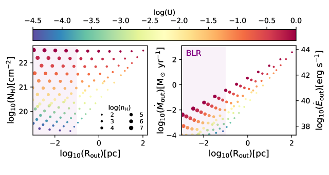
Figure 7: Photoionization modeling with Cloudy. (Left) Inferred possible hydrogen column density of the He i absorber is plotted as a function of size. Each point represents a single model, where the color and size indicate the density and ionization parameter of that model, respectively. The purple shaded region covers sizes $<$ 0.1pc which would approximately represent an origin within the AGN broad line region. (Right) Inferred mass outflow rates are shown in the same manner. The possible mass outflow rates span 6 orders of magnitude, primarily due to the unknown gas density.

4.6 Black Hole Mass

The various scaling relations consistently result in black hole masses in the range $\sim 10^{7.9}-10^{8.6}~{}{\rm M}_{\odot}$. This black hole mass is lower than typical UV-selected quasars at $z\sim 3$ (e.g., Shen & Kelly, 2012), but, as it is roughly $8-40$% of the stellar mass, similar to the unexpected large black hole to stellar mass ratios found at higher redshifts (Goulding et al., 2023; Maiolino et al., 2023).

If we adopt the narrow line widths as $\sigma_{\rm gas}=200-270$ km/s, then we find an expected range of $M_{\rm BH}=4\times 10^{7}-2\times 10^{8}~{}{\rm M}_{\odot}$. These values are consistent with our broad-line scalings, suggesting that while the stellar mass may be catching up, the black hole may still scale with the stellar velocity dispersion (Chisholm et al., 2003; Maiolino et al., 2023).

Given the range of black hole masses, we obtain an Eddington luminosity of $\sim 2-13\times 10^{12}~{}{\rm L}_{\odot}$, implying the black hole radiates at $\sim 40$% of the Eddington limit to potentially super-Eddington.

However, we caution that systematic uncertainties, including the intrinsic scatter in the scaling relations and different dust models, which are not accounted for, likely dominate the error budget at $\gtrsim 1$ dex level for the above estimations.

4.7 X-ray Non-detection

RUBIES-BLAGN-1 was observed by the Chandra X-ray Observatory in Cycle 17, as presented by Kocevski et al. (2018). We adopt the exposure maps, event rates, and PSF models from those authors. At the position of RUBIES-BLAGN-1, the effective exposure time is $\approx 170$ ks using the Advanced CCD Imaging Spectrometer-I. Assuming a standard power-law slope of $\Gamma=1.9$ at $z=3$ (Wang et al., 2021) and foreground galactic absorption $N_{\rm H}=2.01\times 10^{20}~{}{\rm cm}^{-2}$, we directly measure the restframe 2-10 keV counts at the position of the source. The resulting $3\sigma$ upper limit $<3\times 10^{43}~{}{\rm erg\,s^{-1}}$, making the source nearly 100 times fainter than we would naively expect from the dereddened $L_{5100}$ luminosity of $\sim 10^{46}~{}{\rm erg\,s^{-1}}$. This surprising result is discussed further in Section 5.1.

5 Discussion and Conclusions

We present spectroscopic observations of a bright IR-luminous broad-line LRD using NIRSpec/Prism and G395M onboard JWST. We perform spectrophotometric modeling to infer the properties of the host galaxy and the AGN, and decompose the emission and absorption complexes to constrain the gas kinematics and measure the black hole mass. Additionally, we take a first look at the mass outflow rate as implied from the He i $\lambda$ 1.083$\mu$m absorption. Below we discuss the key findings in this work.

5.1 A Spectroscopically Confirmed Broad-Line AGN with a Deficit of Hot Dust

RUBIES-BLAGN-1 is an unusually red and bright object compared to the parent RUBIES sample. In this paper, we argue that the bright and red rest-frame optical continuum is likely dominated by AGN light. The presence of an AGN is supported by the broad and symmetric Balmer and Paschen emission lines, strongly suggesting that we are seeing the AGN disk and broad-line region directly (i.e., an unobscured, but highly reddened AGN). In combination with the lack of broadened forbidden lines, the data disfavor an outflow interpretation.

We have developed a novel method to model the host galaxy and AGN within the Prospector Bayesian inference framework (Johnson et al., 2021). Our preferred model is a composite AGN+host model, in which the UV and the Balmer break are explained by galaxy light, and the AGN continuum from the outer accretion disk dominates in the optical and mid-IR. We find that explaining the rest-frame optical continuum light with pure galaxy continuum is possible, but yields a very high mass of $\sim 10^{11}~{}{\rm M}_{\odot}$. While unresolved in the rest-frame optical, its measured half light radius ($<0.27$ kpc at F277W) would yield an extreme stellar surface density $>10^{12.4}$ ${\rm M}_{\odot}$ kpc^-2; even a conservative upper limit of one pixel on its size would yield a very high stellar density $>10^{11.2}$ ${\rm M}_{\odot}$ kpc^-2 (in some tension with theoretical density limits from stellar feedback; Hopkins et al., 2010; Grudić et al., 2019) and is inconsistent with the dynamical mass inferred from the narrow Pa-$\gamma$ and Pa-$\delta$ emission lines. Further, a galaxy interpretation also would lead to a very high H$\alpha$ rest-frame EW of $\sim 800$Å, which is inconsistent with the inferred older stellar populations and also has not been seen in known AGNs (Vanden Berk et al., 2001; Stern & Laor, 2012). Likewise, fitting a pure AGN model fails to reproduce the spectral shape around the Balmer break region (see Appendix A).

It is worth emphasizing, however, that we cannot rule out a small fraction of the red light coming from a massive galaxy with an older dusty stellar population. This additional stellar component would contribute a lot more mass, potentially amounting to a stellar mass at the order of $10^{10}~{}{\rm M}_{\odot}$, without violating the main conclusions of a prominent AGN.

The flat (in $F_{\nu}$) spectral shape in the mid-IR also presents a significant challenge to our composite AGN and host galaxy picture since a near-ubiquitous component of AGN at all redshifts is a hot dusty torus that begins to dominate AGN emission longward of 2 $\micron$. That component is not observed in this source. In fact, a much larger sample of sources detected in the JADES fields tells the same basic story; while the rest-frame optical appears to require significant obscuration, there is no evidence of emission from the torus itself out to $2-5~{}\micron$ in the rest frame (Williams et al., 2023; Pérez-González et al., 2024). In the majority of cases, with the exception of one object from Matthee et al. (2023), this larger sample do not have measurements of broad H$\alpha$, and so RUBIES-BLAGN-1 provides a special case where we can strongly argue for an AGN component despite the lack of hot dust, perhaps refuting the assumption made in Pérez-González et al. (2024) that these sources are best explained by dusty star formation in the majority of cases. However, RUBIES-BLAGN-1 provides clear confirmation that it is possible to both have an unambiguous broad-line AGN dominate the red continuum in the rest frame optical and simultaneously lack the rising hot dust continuum in the mid-infrared.

There is another other major puzzle in the SEDs of the LRDs, which is their apparent lack of X-ray emission. Roughly speaking, RUBIES-BLAGN-1 is at least 100 times fainter in the X-ray than we would naively expect from the dereddened $L_{5100}$. Put together, the dusty optical continuum, lack of hot dust, and lack of X-ray emission mean that while we can fit the observed UV-optical SED, we do not yet have a full understanding of the underlying physical picture. Thus, measurements of the extinction, intrinsic AGN luminosity, and black hole mass should all be viewed as contingent until a more complete picture can be built.

Even considering a wider redshift range, there are limited number of known analog AGNs with this particular set of spectral characteristics. A handful of cases with a deficiency of hot dust emission are known among high-redshift QSOs (Jiang et al., 2010). These are thought to have evolved relatively dust-poor due to their early formation, although similar hot dust deficient AGN also exist at low-z (Hao et al., 2011; Lyu et al., 2017; Brown et al., 2019; Son et al., 2023). No consensus yet exists about the physical origin of the hot dust deficiency, although a potential explanation could be a difference in torus structure (see discussion in Lyu & Rieke, 2022). However, known dust-deficient AGNs are also typically blue in the rest-frame optical reflecting low dust obscuration, in stark contrast to the extreme red rest-optical colors of our confirmed RUBIES-BLAGN-1 and LRDs in the literature. Meanwhile, analogous low-luminosity AGN with similarly v-shaped SEDs in the rest-optical/UV (e.g., blue dust obscured galaxies; Noboriguchi et al. 2023) tend to get hot quickly, and are heavily obscured at rest-frame $<6~{}\mu$m, leading to steeply rising SEDs into the mid-IR. While it could be possible to reconcile these inconsistent SED properties for specific host geometries that strongly attenuate the rest-optical without an obscuring dust torus (e.g., through polar dust instead; Asmus et al. 2016; Stalevski et al. 2019), the fact that statistical samples of LRDs in the literature also exhibit flat mid-IR SEDs (Williams et al., 2023) argues against orientation or geometrical effects giving rise to such unusual SEDs. Thus, to our knowledge, no known class of AGN across redshifts exhibit similar properties to RUBIES-BLAGN-1 and other LRDs.

5.2 Black hole–galaxy Scaling Relations

Other LRD observations have raised an additional challenge in terms of black hole to galaxy scaling relations. Because the sources are selected to be compact, even at high density there is a limit to their stellar mass. Providing our dust corrections are correct, we infer high ratios of black hole to galaxy mass. However, because of the high spectral resolution observations of RUBIES-BLAGN-1, we have an estimate of $\sigma_{*}$ based on the narrow line widths. Much like the broad-line sources highlighted in Maiolino et al. (2023), we see some evidence that the black hole mass is in accord with local $M_{\rm BH}-\sigma_{*}$ scaling relations, even if the stellar mass has not yet caught up. With only a handful of objects it is hard to draw any concrete conclusions yet, but perhaps these relations support the suggestion of Silk et al. (2024) that the high densities in these early galaxies trigger black hole growth and star formation.

5.3 An Ionized Outflow Traced by He I Absorption

We have reported a detection of an absorption feature in the wings of He i $\lambda$ 1.083 $\mu$m in the G395M spectrum. Being in the rest-frame near-IR, studies on this line are scarce, even in nearby objects (Hutchings et al., 2002; Leighly et al., 2011; Zhang et al., 2017; Landt et al., 2019; Wildy et al., 2021). At higher redshifts, outflows in AGN have mainly been probed in the highly ionized phase (e.g., C iv absorption or [O iii] emission), while results on neutral gas emission ([C ii]) have yielded ambiguous results (e.g., Bischetti et al., 2019; Novak et al., 2020). Our observation thus offers a new look at the outflow properties of LRDs.

The ionized gas outflow in RUBIES-BLAGN-1 has a similar velocity to emission line outflows detected in AGN host galaxies at $z\sim$ 2 (e.g., Förster Schreiber et al., 2019), but the physical scale of the outflow appears to be much smaller ($\lesssim$ 100 pc). However, the size of the outflow is poorly constrained in our analysis because the He i absorption strength is virtually independent of the gas density (e.g., Ji et al., 2015).

The most powerful outflow in our model grid has a kinetic luminosity $<$ 1% of the bolometric luminosity ($\sim 10^{47}~{}{\rm erg\,s^{-1}}$). This suggests that this outflow alone is unlikely to be a significant source of feedback, including regulating accretion onto the black hole or star formation in the host galaxy, but there may be additional outflow mass hidden in other phases (Belli et al., 2023).

In the future, observations covering the H$\alpha$ or H$\beta$ line at higher spectral resolution would help to better constrain the gas density in the absorbing material (e.g., Wildy et al., 2016). Measurements of absorption column densities in lower ionization absorption lines such as Na i d would also provide stronger constraints on the ionization structure within the absorbing medium. In addition, higher resolution observations covering [O iii] $\lambda$ 5007 (Liu et al., 2013) would allow us to search for larger scale ionized outflows manifesting as broad forbidden emission line components and examine the relationship between these kpc-scale outflows and the smaller He i outflow seen in our observations.

5.4 Final Remarks

The red objects discovered by JWST continue to challenge the standard views surrounding the evolution of black holes and galaxies. This paper presents an in-depth analysis of an LRD that has both broad lines and JWST/MIRI detections, an occurrence that was observed only once previously. While it remains uncertain whether RUBIES-BLAGN-1 represents the typical properties of LRDs in terms of the inferred characteristics of the host galaxy, AGN, and outflows, this work demonstrates a promising prospect for understanding the nature of the red sources. The RUBIES program will obtain a statistical sample in the near future, and we plan to extend our modeling framework to perform a systematic investigation, which will contribute to complete an important chapter of the narrative of black hole growth.

Appendix

A Alternative SED Models

Four alternative SED models are considered to offer insight into the systematic uncertainties. The inferred key parameters from each model are summarized in Table 4. The galaxy-only model, which is used to argue in favor of our fiducial composite model in Section 4.1, is not discussed again here.

Table 4: Inferred Key Parameters Assuming Alternative SED Models

Parameter	Galaxy-only	AGN-only	Two-component Dust	UV Continuum Masked
log $M_{*}/{\rm M}_{\odot}$	$11.23_{-0.05}^{+0.05}$	–	$9.62_{-0.17}^{+0.14}$	$9.63^{+0.20}_{-0.24}$
Age [Gyr]	$0.81_{-0.18}^{+0.14}$	–	$1.05_{-0.39}^{+0.13}$	$0.62^{+0.13}_{-0.11}$
SFR [${\rm M}_{\odot}\,{\rm yr}^{-1}$]	$60.88_{-16.06}^{+19.99}$	–	$1.42_{-0.38}^{+0.67}$	$0.72^{+0.83}_{-0.59}$
log sSFR/${\rm yr}^{-1}$	$-9.74_{-0.16}^{+0.15}$	–	$-9.89_{-0.21}^{+0.40}$	$-10.06^{+0.46}_{-0.88}$
log $Z/{\rm Z}_{\odot}$	$-0.08_{-0.14}^{+0.12}$	–	$-1.24_{-0.25}^{+0.23}$	$-1.35^{+0.29}_{-0.27}$
$\hat{\tau}_{\rm dust,1}$	$0.01_{-0.00}^{+0.01}$	–	$2.72_{-0.46}^{+0.54}$	–
$f_{\rm obrun}$	$0.71^{+0.03}_{-0.02}$	–	$0.09_{-0.06}^{+0.11}$	–
$\hat{\tau}_{\rm dust,2}$	$2.69_{-0.13}^{+0.12}$	$3.14_{-0.24}^{+0.17}$	$3.65_{-0.13}^{+0.12}$	$0.72^{+0.14}_{-0.19}$
$n_{\rm dust,2}$	$0.18_{-0.06}^{+0.06}$	$0.02_{-0.02}^{+0.03}$	$-0.27_{-0.04}^{+0.03}$	$-0.91^{+0.12}_{-0.06}$
$f_{\rm nodust}$	$0.00_{-0.00}^{+0.00}$	$0.50_{-0.26}^{+0.19}$	$0.58_{-0.14}^{+0.12}$	$0.12^{+0.16}_{-0.09}$
$\log f_{\rm AGN,7500A}$	–	–	$0.94_{-0.13}^{+0.21}$	$0.86^{+0.20}_{-0.17}$
$f_{\rm AGN,torus}$	–	–	$0.04_{-0.03}^{+0.23}$	$0.02^{+0.31}_{-0.02}$
$\hat{\tau}_{\rm torus}$	–	–	$15.91_{-6.25}^{+14.05}$	$18.40_{-10.34}^{+23.63}$
$\hat{\tau}_{\rm dust,4}$	–	$0.52_{-0.18}^{+0.29}$	–	$3.60^{+0.16}_{-0.19}$
$n_{\rm dust,4}$	–	$-1.07_{-0.13}^{+0.12}$	–	$-0.89^{+0.10}_{-0.07}$

A.1 AGN Only

We construct a simple AGN model, composed solely of accretion disk and torus emissions. The best-fit is shown in Figures 8 (a). This AGN-only model fails to describe the blue UV slope, as expected given the intrinsic spectral shape of the AGN accretion disk. Combining this result with the galaxy-only model supports the inference from our fiducial model that the observed spectrum of RUBIES-BLAGN-1 comprises light from the AGN and its host galaxy. We note, however, that a pure-AGN model with a scattered light component (Greene et al., 2023) remains a possibility.

A.2 Dust

The redness of RUBIES-BLAGN-1 does not necessarily mean that the AGN receives additional attenuation. We thus consider the standard dust model, where dust reddening of the stellar light is described by two components (Charlot & Fall, 2000) with a flexible dust attenuation curve (Noll et al., 2009). As in the fiducial model, a fraction of the stellar light is allowed to be seen outside the diffuse dust. In addition, a fraction of the young stellar light is allowed to be not attenuated by the birth cloud, which represents runaway OB stars or escaping ionizing radiation.

This model infers significant dust presence, driven by the red continuum as in the fiducial model. However, without the additional attenuation experienced only by the AGN, $\sim 10$% of the young stars and $\sim 60$% of all stars are required to be located outside the birth cloud and the diffuse dust, respectively, to produce the UV excess. It is less intuitive to reconcile this situation where a significant fraction of the stars remains unaffected by dust attenuation while the AGN experiences substantial attenuation.

A.3 Fitting the Rest Optical Spectrum Only

It is possible that the UV continuum is of non-stellar origin. We test this hypothesis by masking the UV, and fit the red continuum with the fiducial model. This setting fails to predict an UV excess, meaning that the UV continuum does not have to be composed of starlight. It can, for example, be the scattered light from the AGN (Greene et al., 2023). Crucially, the inferred stellar mass in this case is about the same as that from the fiducial model, suggesting that the UV continuum has less constraining power. While we can add in a non-stellar component for the UV, this result means that the extra UV component will not add much information under the assumed dust model, except improving the $\chi^{2}$.

Figure 8: Alternative SED models. (a) Fitting with AGN light only. (b) Fitting with the standard two-component dust model. (c) Fitting only the rest optical spectrum using the fiducial model. In each panel, the best-fit total model spectrum, with the marginalized emission lines added, is plotted in orange. The model spectra of the AGN accretion disk, torus, and the galaxy are plotted in red, pink, and blue, respectively. The photometric observations are included as black dots, but the observed spectrum is omitted for clarity.

References

- Abramowicz et al. (1988) Abramowicz, M. A., Czerny, B., Lasota, J. P., & Szuszkiewicz, E. 1988, ApJ, 332, 646, doi: 10.1086/166683
- Asmus et al. (2016) Asmus, D., Hönig, S. F., & Gandhi, P. 2016, ApJ, 822, 109, doi: 10.3847/0004-637X/822/2/109
- Astropy Collaboration et al. (2022) Astropy Collaboration, Price-Whelan, A. M., Lim, P. L., et al. 2022, ApJ, 935, 167, doi: 10.3847/1538-4357/ac7c74
- Baggen et al. (2023) Baggen, J. F. W., van Dokkum, P., Labbé, I., et al. 2023, ApJ, 955, L12, doi: 10.3847/2041-8213/acf5ef
- Barro et al. (2023) Barro, G., Perez-Gonzalez, P. G., Kocevski, D. D., et al. 2023, arXiv e-prints, arXiv:2305.14418, doi: 10.48550/arXiv.2305.14418
- Barrufet et al. (2023) Barrufet, L., Oesch, P. A., Weibel, A., et al. 2023, MNRAS, 522, 449, doi: 10.1093/mnras/stad947
- Belli et al. (2023) Belli, S., Park, M., Davies, R. L., et al. 2023, arXiv e-prints, arXiv:2308.05795, doi: 10.48550/arXiv.2308.05795
- Bertin & Arnouts (1996) Bertin, E., & Arnouts, S. 1996, A&AS, 117, 393, doi: 10.1051/aas:1996164
- Bischetti et al. (2019) Bischetti, M., Maiolino, R., Carniani, S., et al. 2019, A&A, 630, A59, doi: 10.1051/0004-6361/201833557
- Blandford & McKee (1982) Blandford, R. D., & McKee, C. F. 1982, ApJ, 255, 419, doi: 10.1086/159843
- Bosman et al. (2023) Bosman, S. E. I., Álvarez-Márquez, J., Colina, L., et al. 2023, arXiv e-prints, arXiv:2307.14414, doi: 10.48550/arXiv.2307.14414
- Brammer (2023a) Brammer, G. 2023a, grizli, 1.9.11, Zenodo, doi: 10.5281/zenodo.1146904
- Brammer (2023b) —. 2023b, msaexp: NIRSpec analyis tools, 0.6.17, Zenodo, doi: 10.5281/zenodo.7299500
- Brown et al. (2019) Brown, M. J. I., Duncan, K. J., Landt, H., et al. 2019, MNRAS, 489, 3351, doi: 10.1093/mnras/stz2324
- Calzetti et al. (2000) Calzetti, D., Armus, L., Bohlin, R. C., et al. 2000, ApJ, 533, 682, doi: 10.1086/308692
- Cappellari et al. (2006) Cappellari, M., Bacon, R., Bureau, M., et al. 2006, MNRAS, 366, 1126, doi: 10.1111/j.1365-2966.2005.09981.x
- Carnall et al. (2023) Carnall, A. C., McLure, R. J., Dunlop, J. S., et al. 2023, Nature, 619, 716, doi: 10.1038/s41586-023-06158-6
- Chabrier (2003) Chabrier, G. 2003, PASP, 115, 763, doi: 10.1086/376392
- Charlot & Fall (2000) Charlot, S., & Fall, S. M. 2000, ApJ, 539, 718, doi: 10.1086/309250
- Chatzikos et al. (2023) Chatzikos, M., Bianchi, S., Camilloni, F., et al. 2023, Rev. Mexicana Astron. Astrofis., 59, 327, doi: 10.22201/ia.01851101p.2023.59.02.12
- Chisholm et al. (2003) Chisholm, J. R., Dodelson, S., & Kolb, E. W. 2003, ApJ, 596, 437, doi: 10.1086/377628
- Choi et al. (2016) Choi, J., Dotter, A., Conroy, C., et al. 2016, ApJ, 823, 102, doi: 10.3847/0004-637X/823/2/102
- Conroy & Gunn (2010) Conroy, C., & Gunn, J. E. 2010, ApJ, 712, 833, doi: 10.1088/0004-637X/712/2/833
- Conroy et al. (2009) Conroy, C., Gunn, J. E., & White, M. 2009, ApJ, 699, 486, doi: 10.1088/0004-637X/699/1/486
- Culliton et al. (2019) Culliton, C., Charlton, J., Eracleous, M., Ganguly, R., & Misawa, T. 2019, MNRAS, 488, 4690, doi: 10.1093/mnras/stz1642
- Davies et al. (2020) Davies, R., Baron, D., Shimizu, T., et al. 2020, MNRAS, 498, 4150, doi: 10.1093/mnras/staa2413
- de Graaff et al. (2023) de Graaff, A., Rix, H.-W., Carniani, S., et al. 2023, arXiv e-prints, arXiv:2308.09742, doi: 10.48550/arXiv.2308.09742
- Dotter (2016) Dotter, A. 2016, ApJS, 222, 8, doi: 10.3847/0067-0049/222/1/8
- Draine & Li (2007) Draine, B. T., & Li, A. 2007, ApJ, 657, 810, doi: 10.1086/511055
- Dullemond & van Bemmel (2005) Dullemond, C. P., & van Bemmel, I. M. 2005, A&A, 436, 47, doi: 10.1051/0004-6361:20041763
- Eenens & Williams (1994) Eenens, P. R. J., & Williams, P. M. 1994, MNRAS, 269, 1082, doi: 10.1093/mnras/269.4.1082
- Eisenstein et al. (2023) Eisenstein, D. J., Willott, C., Alberts, S., et al. 2023, arXiv e-prints, arXiv:2306.02465, doi: 10.48550/arXiv.2306.02465
- Ferland et al. (2017) Ferland, G. J., Chatzikos, M., Guzmán, F., et al. 2017, Rev. Mexicana Astron. Astrofis., 53, 385, doi: 10.48550/arXiv.1705.10877
- Foreman-Mackey (2016) Foreman-Mackey, D. 2016, The Journal of Open Source Software, 1, 24, doi: 10.21105/joss.00024
- Foreman-Mackey et al. (2013) Foreman-Mackey, D., Hogg, D. W., Lang, D., & Goodman, J. 2013, PASP, 125, 306, doi: 10.1086/670067
- Förster Schreiber et al. (2019) Förster Schreiber, N. M., Übler, H., Davies, R. L., et al. 2019, ApJ, 875, 21, doi: 10.3847/1538-4357/ab0ca2
- Furtak et al. (2023a) Furtak, L. J., Zitrin, A., Plat, A., et al. 2023a, ApJ, 952, 142, doi: 10.3847/1538-4357/acdc9d
- Furtak et al. (2023b) Furtak, L. J., Labbé, I., Zitrin, A., et al. 2023b, arXiv e-prints, arXiv:2308.05735, doi: 10.48550/arXiv.2308.05735
- Goulding et al. (2023) Goulding, A. D., Greene, J. E., Setton, D. J., et al. 2023, ApJ, 955, L24, doi: 10.3847/2041-8213/acf7c5
- Greene & Ho (2005) Greene, J. E., & Ho, L. C. 2005, ApJ, 630, 122, doi: 10.1086/431897
- Greene et al. (2023) Greene, J. E., Labbe, I., Goulding, A. D., et al. 2023, arXiv e-prints, arXiv:2309.05714, doi: 10.48550/arXiv.2309.05714
- Grogin et al. (2011) Grogin, N. A., Kocevski, D. D., Faber, S. M., et al. 2011, ApJS, 197, 35, doi: 10.1088/0067-0049/197/2/35
- Grudić et al. (2019) Grudić, M. Y., Hopkins, P. F., Quataert, E., & Murray, N. 2019, MNRAS, 483, 5548, doi: 10.1093/mnras/sty3386
- Hainline et al. (2011) Hainline, L. J., Blain, A. W., Smail, I., et al. 2011, ApJ, 740, 96, doi: 10.1088/0004-637X/740/2/96
- Hao et al. (2011) Hao, C.-N., Kennicutt, R. C., Johnson, B. D., et al. 2011, ApJ, 741, 124, doi: 10.1088/0004-637X/741/2/124
- Hao et al. (2010) Hao, H., Elvis, M., Civano, F., et al. 2010, ApJ, 724, L59, doi: 10.1088/2041-8205/724/1/L59
- Harikane et al. (2023) Harikane, Y., Zhang, Y., Nakajima, K., et al. 2023, ApJ, 959, 39, doi: 10.3847/1538-4357/ad029e
- Harris et al. (2020) Harris, C. R., Millman, K. J., van der Walt, S. J., et al. 2020, Nature, 585, 357, doi: 10.1038/s41586-020-2649-2
- Hinshaw et al. (2013) Hinshaw, G., Larson, D., Komatsu, E., et al. 2013, ApJS, 208, 19, doi: 10.1088/0067-0049/208/2/19
- Hönig et al. (2006) Hönig, S. F., Beckert, T., Ohnaka, K., & Weigelt, G. 2006, A&A, 452, 459, doi: 10.1051/0004-6361:20054622
- Hopkins et al. (2010) Hopkins, P. F., Murray, N., Quataert, E., & Thompson, T. A. 2010, MNRAS, 401, L19, doi: 10.1111/j.1745-3933.2009.00777.x
- Hunter (2007) Hunter, J. D. 2007, Computing in Science and Engineering, 9, 90, doi: 10.1109/MCSE.2007.55
- Hutchings et al. (2002) Hutchings, J. B., Crenshaw, D. M., Kraemer, S. B., et al. 2002, AJ, 124, 2543, doi: 10.1086/344080
- Ji et al. (2015) Ji, T., Zhou, H., Jiang, P., et al. 2015, ApJ, 800, 56, doi: 10.1088/0004-637X/800/1/56
- Ji et al. (2024) Ji, Z., Williams, C. C., Suess, K. A., et al. 2024, arXiv e-prints, arXiv:2401.00934, doi: 10.48550/arXiv.2401.00934
- Jiang et al. (2010) Jiang, L., Fan, X., Brandt, W. N., et al. 2010, Nature, 464, 380, doi: 10.1038/nature08877
- Johnson et al. (2021) Johnson, B. D., Leja, J., Conroy, C., & Speagle, J. S. 2021, ApJS, 254, 22, doi: 10.3847/1538-4365/abef67
- Kaspi et al. (2000) Kaspi, S., Smith, P. S., Netzer, H., et al. 2000, ApJ, 533, 631, doi: 10.1086/308704
- Killi et al. (2023) Killi, M., Watson, D., Brammer, G., et al. 2023, arXiv e-prints, arXiv:2312.03065, doi: 10.48550/arXiv.2312.03065
- Kim et al. (2015) Kim, D., Im, M., Glikman, E., Woo, J.-H., & Urrutia, T. 2015, ApJ, 812, 66, doi: 10.1088/0004-637X/812/1/66
- Kim et al. (2010) Kim, D., Im, M., & Kim, M. 2010, ApJ, 724, 386, doi: 10.1088/0004-637X/724/1/386
- Kocevski et al. (2018) Kocevski, D. D., Hasinger, G., Brightman, M., et al. 2018, ApJS, 236, 48, doi: 10.3847/1538-4365/aab9b4
- Kocevski et al. (2023) Kocevski, D. D., Onoue, M., Inayoshi, K., et al. 2023, ApJ, 954, L4, doi: 10.3847/2041-8213/ace5a0
- Koekemoer et al. (2011) Koekemoer, A. M., Faber, S. M., Ferguson, H. C., et al. 2011, ApJS, 197, 36, doi: 10.1088/0067-0049/197/2/36
- Kokorev et al. (2023) Kokorev, V., Fujimoto, S., Labbe, I., et al. 2023, ApJ, 957, L7, doi: 10.3847/2041-8213/ad037a
- Kubota & Done (2019) Kubota, A., & Done, C. 2019, MNRAS, 489, 524, doi: 10.1093/mnras/stz2140
- Labbé et al. (2023a) Labbé, I., Greene, J. E., Bezanson, R., et al. 2023a, arXiv e-prints, arXiv:2306.07320, doi: 10.48550/arXiv.2306.07320
- Labbé et al. (2023b) Labbé, I., van Dokkum, P., Nelson, E., et al. 2023b, Nature, 616, 266, doi: 10.1038/s41586-023-05786-2
- Lacy et al. (2004) Lacy, M., Storrie-Lombardi, L. J., Sajina, A., et al. 2004, ApJS, 154, 166, doi: 10.1086/422816
- Laha et al. (2021) Laha, S., Reynolds, C. S., Reeves, J., et al. 2021, Nature Astronomy, 5, 13, doi: 10.1038/s41550-020-01255-2
- Landt et al. (2013) Landt, H., Ward, M. J., Peterson, B. M., et al. 2013, MNRAS, 432, 113, doi: 10.1093/mnras/stt421
- Landt et al. (2019) Landt, H., Ward, M. J., Kynoch, D., et al. 2019, MNRAS, 489, 1572, doi: 10.1093/mnras/stz2212
- Laurent et al. (2000) Laurent, O., Mirabel, I. F., Charmandaris, V., et al. 2000, A&A, 359, 887, doi: 10.48550/arXiv.astro-ph/0005376
- Leighly et al. (2011) Leighly, K. M., Dietrich, M., & Barber, S. 2011, ApJ, 728, 94, doi: 10.1088/0004-637X/728/2/94
- Leja et al. (2018) Leja, J., Johnson, B. D., Conroy, C., & van Dokkum, P. 2018, ApJ, 854, 62, doi: 10.3847/1538-4357/aaa8db
- Leja et al. (2017) Leja, J., Johnson, B. D., Conroy, C., van Dokkum, P. G., & Byler, N. 2017, ApJ, 837, 170, doi: 10.3847/1538-4357/aa5ffe
- Libralato et al. (2023) Libralato, M., Argyriou, I., Dicken, D., et al. 2023, arXiv e-prints, arXiv:2311.12145, doi: 10.48550/arXiv.2311.12145
- Liu et al. (2013) Liu, G., Zakamska, N. L., Greene, J. E., Nesvadba, N. P. H., & Liu, X. 2013, MNRAS, 436, 2576, doi: 10.1093/mnras/stt1755
- Lyu & Rieke (2022) Lyu, J., & Rieke, G. 2022, Universe, 8, 304, doi: 10.3390/universe8060304
- Lyu et al. (2017) Lyu, J., Rieke, G. H., & Shi, Y. 2017, ApJ, 835, 257, doi: 10.3847/1538-4357/835/2/257
- Maiolino et al. (2023) Maiolino, R., Scholtz, J., Curtis-Lake, E., et al. 2023, arXiv e-prints, arXiv:2308.01230, doi: 10.48550/arXiv.2308.01230
- Mathews & Ferland (1987) Mathews, W. G., & Ferland, G. J. 1987, ApJ, 323, 456, doi: 10.1086/165843
- Matthee et al. (2023) Matthee, J., Naidu, R. P., Brammer, G., et al. 2023, arXiv e-prints, arXiv:2306.05448, doi: 10.48550/arXiv.2306.05448
- Misawa et al. (2007) Misawa, T., Charlton, J. C., Eracleous, M., et al. 2007, ApJS, 171, 1, doi: 10.1086/513713
- Mor & Trakhtenbrot (2011) Mor, R., & Trakhtenbrot, B. 2011, ApJ, 737, L36, doi: 10.1088/2041-8205/737/2/L36
- Nenkova et al. (2008a) Nenkova, M., Sirocky, M. M., Ivezić, Ž., & Elitzur, M. 2008a, ApJ, 685, 147, doi: 10.1086/590482
- Nenkova et al. (2008b) Nenkova, M., Sirocky, M. M., Nikutta, R., Ivezić, Ž., & Elitzur, M. 2008b, ApJ, 685, 160, doi: 10.1086/590483
- Noboriguchi et al. (2023) Noboriguchi, A., Inoue, A. K., Nagao, T., Toba, Y., & Misawa, T. 2023, ApJ, 959, L14, doi: 10.3847/2041-8213/ad0e00
- Noll et al. (2009) Noll, S., Burgarella, D., Giovannoli, E., et al. 2009, A&A, 507, 1793, doi: 10.1051/0004-6361/200912497
- Novak et al. (2020) Novak, M., Venemans, B. P., Walter, F., et al. 2020, ApJ, 904, 131, doi: 10.3847/1538-4357/abc33f
- Pacucci & Loeb (2024) Pacucci, F., & Loeb, A. 2024, arXiv e-prints, arXiv:2401.04159, doi: 10.48550/arXiv.2401.04159
- Pan et al. (2019) Pan, X., Zhou, H., Liu, W., et al. 2019, ApJ, 883, 173, doi: 10.3847/1538-4357/ab40b5
- Pasha & Miller (2023) Pasha, I., & Miller, T. B. 2023, The Journal of Open Source Software, 8, 5703, doi: 10.21105/joss.05703
- Pérez-González et al. (2024) Pérez-González, P. G., Barro, G., Rieke, G. H., et al. 2024, arXiv e-prints, arXiv:2401.08782, doi: 10.48550/arXiv.2401.08782
- Richards et al. (2006) Richards, G. T., Lacy, M., Storrie-Lombardi, L. J., et al. 2006, ApJS, 166, 470, doi: 10.1086/506525
- Rupke et al. (2005) Rupke, D. S., Veilleux, S., & Sanders, D. B. 2005, ApJS, 160, 115, doi: 10.1086/432889
- Rupke et al. (2017) Rupke, D. S. N., Gültekin, K., & Veilleux, S. 2017, ApJ, 850, 40, doi: 10.3847/1538-4357/aa94d1
- Sánchez-Blázquez et al. (2006) Sánchez-Blázquez, P., Peletier, R. F., Jiménez-Vicente, J., et al. 2006, MNRAS, 371, 703, doi: 10.1111/j.1365-2966.2006.10699.x
- Sanders et al. (1989) Sanders, D. B., Phinney, E. S., Neugebauer, G., Soifer, B. T., & Matthews, K. 1989, ApJ, 347, 29, doi: 10.1086/168094
- Savage & Sembach (1991) Savage, B. D., & Sembach, K. R. 1991, ApJ, 379, 245, doi: 10.1086/170498
- Sawicki (2002) Sawicki, M. 2002, AJ, 124, 3050, doi: 10.1086/344682
- Setton et al. (2024) Setton, D. J., Khullar, G., Miller, T. B., et al. 2024, arXiv e-prints, arXiv:2402.05664, doi: 10.48550/arXiv.2402.05664
- Shen et al. (2020) Shen, X., Hopkins, P. F., Faucher-Giguère, C.-A., et al. 2020, MNRAS, 495, 3252, doi: 10.1093/mnras/staa1381
- Shen & Kelly (2012) Shen, Y., & Kelly, B. C. 2012, ApJ, 746, 169, doi: 10.1088/0004-637X/746/2/169
- Silk et al. (2024) Silk, J., Begelman, M. C., Norman, C., Nusser, A., & Wyse, R. F. G. 2024, ApJ, 961, L39, doi: 10.3847/2041-8213/ad1bf0
- Son et al. (2023) Son, S., Kim, M., & Ho, L. C. 2023, ApJ, 953, 175, doi: 10.3847/1538-4357/ace165
- Speagle (2020) Speagle, J. S. 2020, MNRAS, 493, 3132, doi: 10.1093/mnras/staa278
- Speagle et al. (2014) Speagle, J. S., Steinhardt, C. L., Capak, P. L., & Silverman, J. D. 2014, ApJS, 214, 15, doi: 10.1088/0067-0049/214/2/15
- Stalevski et al. (2019) Stalevski, M., Tristram, K. R. W., & Asmus, D. 2019, MNRAS, 484, 3334, doi: 10.1093/mnras/stz220
- Stern & Laor (2012) Stern, J., & Laor, A. 2012, MNRAS, 423, 600, doi: 10.1111/j.1365-2966.2012.20901.x
- Stevens & Howarth (1999) Stevens, I. R., & Howarth, I. D. 1999, MNRAS, 302, 549, doi: 10.1046/j.1365-8711.1999.02151.x
- Temple et al. (2021) Temple, M. J., Hewett, P. C., & Banerji, M. 2021, MNRAS, 508, 737, doi: 10.1093/mnras/stab2586
- Urrutia et al. (2012) Urrutia, T., Lacy, M., Spoon, H., et al. 2012, ApJ, 757, 125, doi: 10.1088/0004-637X/757/2/125
- Valentino et al. (2023) Valentino, F., Brammer, G., Gould, K. M. L., et al. 2023, ApJ, 947, 20, doi: 10.3847/1538-4357/acbefa
- Vanden Berk et al. (2001) Vanden Berk, D. E., Richards, G. T., Bauer, A., et al. 2001, AJ, 122, 549, doi: 10.1086/321167
- Vidal-García et al. (2024) Vidal-García, A., Plat, A., Curtis-Lake, E., et al. 2024, MNRAS, 527, 7217, doi: 10.1093/mnras/stad3252
- Virtanen et al. (2020) Virtanen, P., Gommers, R., Oliphant, T. E., et al. 2020, Nature Methods, 17, 261, doi: 10.1038/s41592-019-0686-2
- Wang et al. (2023a) Wang, B., Fujimoto, S., Labbé, I., et al. 2023a, ApJ, 957, L34, doi: 10.3847/2041-8213/acfe07
- Wang et al. (2023b) Wang, B., Leja, J., Bezanson, R., et al. 2023b, ApJ, 944, L58, doi: 10.3847/2041-8213/acba99
- Wang et al. (2024) Wang, B., Leja, J., Labbé, I., et al. 2024, ApJS, 270, 12, doi: 10.3847/1538-4365/ad0846
- Wang et al. (2021) Wang, F., Fan, X., Yang, J., et al. 2021, ApJ, 908, 53, doi: 10.3847/1538-4357/abcc5e
- Whitaker et al. (2014) Whitaker, K. E., Franx, M., Leja, J., et al. 2014, ApJ, 795, 104, doi: 10.1088/0004-637X/795/2/104
- Wildy et al. (2016) Wildy, C., Landt, H., Goad, M. R., Ward, M., & Collinson, J. S. 2016, MNRAS, 461, 2085, doi: 10.1093/mnras/stw1403
- Wildy et al. (2021) Wildy, C., Landt, H., Ward, M. J., Czerny, B., & Kynoch, D. 2021, MNRAS, 500, 2063, doi: 10.1093/mnras/staa3301
- Williams et al. (2023) Williams, C. C., Alberts, S., Ji, Z., et al. 2023, arXiv e-prints, arXiv:2311.07483, doi: 10.48550/arXiv.2311.07483
- Wright et al. (2023) Wright, L., Whitaker, K. E., Weaver, J. R., et al. 2023, arXiv e-prints, arXiv:2311.05394, doi: 10.48550/arXiv.2311.05394
- Yang et al. (2020) Yang, G., Boquien, M., Buat, V., et al. 2020, MNRAS, 491, 740, doi: 10.1093/mnras/stz3001
- Zakamska & Greene (2014) Zakamska, N. L., & Greene, J. E. 2014, MNRAS, 442, 784, doi: 10.1093/mnras/stu842
- Zhang et al. (2017) Zhang, S., Zhou, H., Shi, X., et al. 2017, ApJ, 845, 126, doi: 10.3847/1538-4357/aa8223