Koopman-Assisted Reinforcement Learning

Abstract

The Bellman equation and its continuous form, the Hamilton-Jacobi-Bellman (HJB) equation, are ubiquitous in reinforcement learning (RL) and control theory. However, these equations quickly become intractable for systems with high-dimensional states and nonlinearity. This paper explores the connection between the data-driven Koopman operator and Markov Decision Processes (MDPs), resulting in the development of two new RL algorithms to address these limitations. We leverage Koopman operator techniques to lift a nonlinear system into new coordinates where the dynamics become approximately linear, and where HJB-based methods are more tractable. In particular, the Koopman operator is able to capture the expectation of the time evolution of the value function of a given system via linear dynamics in the lifted coordinates. By parameterizing the Koopman operator with the control actions, we construct a “Koopman tensor” that facilitates the estimation of the optimal value function. Then, a transformation of Bellman’s framework in terms of the Koopman tensor enables us to reformulate two max-entropy RL algorithms: soft value iteration and soft actor-critic (SAC). This highly flexible framework can be used for deterministic or stochastic systems as well as for discrete or continuous-time dynamics. Finally, we show that these Koopman Assisted Reinforcement Learning (KARL) algorithms attain state-of-the-art (SOTA) performance with respect to traditional neural network-based SAC and linear quadratic regulator (LQR) baselines on four controlled dynamical systems: a linear state-space system, the Lorenz system, fluid flow past a cylinder, and a double-well potential with non-isotropic stochastic forcing.

Keywords– Koopman Operator Theory, Reinforcement Learning, Machine Learning, Control Theory, Soft Actor-Critic, Nonlinear Control, Model Predictive Control, Artificial Intelligence, Hamilton-Jacobi-Bellman

1 Introduction

Reinforcement learning (RL) is a rapidly developing field at the intersection of machine learning and control theory, in which an intelligent agent learns how to interact with a complex environment to achieve an objective [1, 2]. Deep reinforcement learning (DRL) [3, 4, 5, 6, 7, 8, 9] has recently been shown capable of achieving human-level or super-human performance in several challenging tasks, including playing video games [10, 11] and strategy games [12, 13, 14]. DRL is also increasingly used for scientific and engineering applications, including for drug discovery [15], robotic manipulation [16], autonomous driving [17] and drone racing [18], fluid flow control [19, 20, 21, 22, 23, 24, 25], and fusion control [26]. Despite this progress, DRL solutions often require tremendous computational resources to train and generalize, and they typically lack interpretability that is critical in many applications.

The algorithms underlying many reinforcement learning strategies are closely related to the Bellman and Hamilton-Jacobi-Bellman equations from optimization and optimal control theory [2]. However, solving these equations becomes intractable for high-dimensional, nonlinear systems, which often motivates the use of deep learning. In this paper, we re-examine the Bellman equation through a novel application of the Koopman operator [27, 28, 29, 30, 31, 32, 33], which allows us to recast a nonlinear dynamical system as a linear system of equations on an infinite-dimensional function space.

Given a deterministic, discrete-time dynamical system

$$x^{\prime}={F}(x)$$ (1)

the Koopman operator provides an alternative perspective in which these dynamics become linear on an infinite-dimensional Hilbert space of measurement functions of the system. Mathematically, given a function from the state space to the reals $g:\mathcal{X}\to\mathbb{R}$, the Koopman operator $\mathcal{K}$ is defined for deterministic (time-homogenous) autonomous systems as:

$$\mathcal{K}g(x):=g({F}(x))=g(x^{\prime}).$$ (2)

More generally, in stochastic autonomous systems, it is defined as the conditional forecast operator:

$$\mathcal{K}g(x) =\mathbb{E}\left(g(X^{\prime})|X=x\right).$$ (3)

This paper recasts the continuation term in the Bellman equation in terms of the Koopman operator, specifically viewing the value function $V^{\pi}(x)$ for a given policy $\pi$ as the Koopman observable. For a deterministic system, the value function may be rewritten using the Koopman operator as:

$$V^{\pi}(x)=r(x,u)+\gamma V^{\pi}(x^{\prime})=r(x,u)+\gamma\mathcal{K}V^{\pi}(x).$$ (4)

In this Koopman formulation, the value function only relies on the current state $x$, whereas in the original formulation it depends on the future state $x^{\prime}$; here, $r$ is the reward function and $\gamma$ is a discount factor. For a stochastic system the value function transforms according to

$$V^{\pi}(x)=\mathbb{E}_{u\sim\pi(\cdot|x)}\left\{r(x,u)+\gamma\mathbb{E}_{x^{\prime}\sim p(\cdot|x,u)}\left[V^{\pi}(x^{\prime})\right]\right\}$$ (5a)

$$\Longrightarrow\quad V^{\pi}(x)=\mathbb{E}_{u\sim\pi(\cdot|x)}\left\{r(x,u)+\gamma\mathcal{K}V^{\pi}(x)\right\}.$$ (5b)

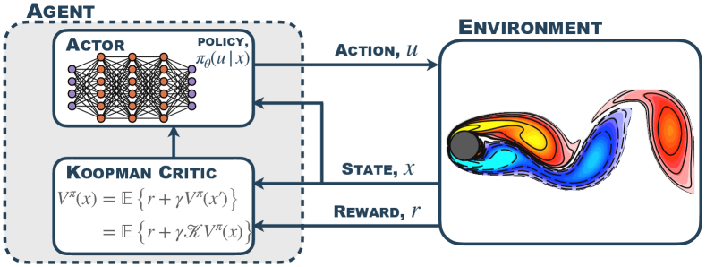
Figure 1: Koopman-assisted reinforcement learning in the example of the Soft Actor Koopman-Critic, a Koopman variant of the popular Soft Actor-Critic algorithm. The Koopman Critic receives the state and the reward in the original state-space, before lifting these variables to a feature space, where the value function can be advanced in time with the Koopman operator. This critique is then fed back to the Actor which issues the action to be performed in the environment. This is 1 of 2 main Koopman-assisted reinforcement learning algorithms explored in this work; the other algorithm is a modified soft Koopman value iteration.

When considering a particular observable, such as the value function in reinforcement learning, it may be possible to learn a finite-dimensional basis, or dictionary, in which this function and its evolution via the Koopman operator can be well approximated. There are many approaches to approximate the Koopman operator from data, such as dynamic mode decomposition (DMD) [34, 35, 36, 37, 38, 39], the extended dynamic mode decomposition (EDMD) [40, 41, 42, 43], and related robust extensions [44, 45, 46]. This body of work was subsequently extended to stochastic dynamical systems [47, 48] and controlled dynamical systems [49, 50, 51]. The correct choice of dictionary space is crucial in Koopman analysis techniques since they are generally not robust to misspecification.

1.1 Contributions

Introduction of two max-entropy RL algorithms using the Koopman operator: soft value iteration [52] and soft actor-critic [53, 54]. We refer to this approach broadly as Koopman-Assisted Reinforcement Learning (KARL) and to the two particular reformulated algorithms as soft Koopman value iteration (SKVI) and soft actor Koopman-critic (SAKC).

Validation of these newly-introduced algorithms on four environments using quadratic cost functions: a linear system, the Lorenz system, fluid flow past a cylinder, and a double-well potential with non-isotropic stochastic forcing.

State-of-the-Art Performance is demonstrated across all four environments compared to state-of-the-art reinforcement learning SAC and classical control LQR baselines.

The Koopman tensor is constructed in a multiplicatively separable dictionary space on states and controls, respectively. This approach extends and generalizes previous attempts to include actuation and control within the Koopman framework. Additionally, the present work extends Koopman for control to the context of Markov decision processes (MDPs).

Extensive ablation analyses for SKVI and SAKC to discern the influence of the dictionary space used for the construction of the Koopman tensor, as well as the influence of the amount of compute used for the construction of the Koopman tensor on the performance of KARL algorithms.

1.2 Related Work

The Koopman operator has recently been applied to RL, with several noteworthy developments. Several works have used the Koopman operator for advancing $Q$ learning, including developing a modified deep $Q$ network (DQN) [55] using imitation learning, and Koopman $Q$-learning based on identifying symmetries in state dynamics [56]. Retchin et al. [57] developed a Koopman constrained policy optimization (KCPO), combining a Koopman autoencoder network with differentiable model predictive control (MPC). Although Koopman autoencoders have been explored for dynamical systems for several years [58, 59, 60, 61, 62, 63], their application in control is recent.

More generally, several studies have extended Koopman analysis from autonomous systems to systems with actuation and control [49, 50, 51]. However, these studies did not extend the Koopman embedding framework to the setting of Markov decision processes (MDPs), which is a main contribution of the present work. Notably, we introduce a new approach to parameterize the Koopman operator using a Koopman tensor on a lifted state-control space, which is essential for handling controlled dynamical systems. The Koopman tensor approach builds upon and extends methods like DMDc [49] and Koopman with inputs and control (KIC) [50] by capturing a wider range of interactions between states and actions. DMDc restricts these interactions to be purely linear and additive, limiting its ability to model complex dynamics; however, the Koopman tensor utilizes Kronecker products between any dictionary spaces, enabling it to capture rich multiplicative and nonlinear relationships. This enhanced flexibility leads to improved model accuracy and allows the Koopman tensor to effectively handle systems with intricate control dependencies. KIC is more general than DMDc, although it requires the prediction of future actions or forcing their predicted values to be zero, which can lead to inaccuracies in predictions of other values. The related sparse identification of nonlinear dynamics with control (SINDYc) algorithm [64, 65] also models controlled dynamical systems. SINDYc offers high flexibility through its generality on the candidate function space for states and controls. In particular, feature maps richer than the multiplicative separable case we consider could be considered with SINDYc.

Some of the earliest work leveraging data-driven Koopman models to design controllers involved the use of DMD and eDMD models for model predictive control [66, 67, 68, 51], with recent extensions including incremental updates [69] and Koopman autoencoders [57]. Importantly, these approaches do not have the same convergence guarantees as KARL. Further, MPC is an extremely robust control architecture that blends model-based feedforward control with sensor-based feedback control. As a result, MPC is often able to achieve robust performance, even with a relatively poor model, as discussed in [65]. It is known that eDMD models often result in spurious eigenvalues and may perform badly with system noise and without tuning, so it is likely that the early Koopman-MPC work was largely exploiting the robustness of MPC rather than the model performance of eDMD. In contrast, KARL approaches rely on having a highly accurate model of the dynamics through the Koopman operator, putting a more more stringent requirement on the model actually predicting the dynamics.

1.3 Outline

In section 2, we discuss the relevant background topics of Koopman operator theory as well as the MDP framework. In section 3, we detail our SKVI and SAKC algorithms. In section 4, we discuss the testing environments, cost functions, and the methods used to evaluate the performance of our KARL algorithms. In section 5, we show the results of the experiments and the performance of the KARL algorithms in the considered environments against SOTA benchmarks in terms of episodic returns. In section 6, we discuss the caveats and limitations of KARL, along with several explicit proposals for how KARL can be improved. In section 7, we summarize and conclude the paper.

2 Background

Here, we discuss relevant background theory and algorithms. We review Koopman operator theory, discuss the reformulation of MDPs, and build intuition that will be used to develop the Koopman tensor in the next section.

2.1 Koopman Operator Theory

Nonlinearity is one of the central challenges in data-driven modeling and control, including modern RL architectures. Koopman operator theory [27, 28, 29, 30, 31, 32, 33] provides an alternative perspective, in which nonlinear dynamics become linear when lifted to an infinite-dimensional Hilbert space of measurement functions of the system. This is consistent with other fields in machine learning, where lifting is known to linearize and simplify otherwise challenging tasks [70].

There are several forms a dynamical system may take to describe the evolution of a state $x$ in time. A deterministic, autonomous system may be written in discrete-time as

$$x^{\prime}={F}(x),$$ (6)

or in continuous-time as

$$\frac{d}{dt}{x}(t)={f}(x(t)).$$ (7)

Every continuous-time system induces a discrete-time system via the flow map operator

$$x(t+\tau)={F}_{\tau}(x(t))=x(t)+\int_{t}^{t+\tau}{f}(x(s))ds.$$

The Koopman operator provides an alternative perspective. Formally, we consider real-valued vector measurement functions $g\colon M\to\mathbb{R}$, which are themselves elements of an infinite-dimensional Hilbert space and where $M$ is a manifold. Typically this manifold is taken to be $L^{\infty}(\mathcal{X})$ where $\mathcal{X}\subset\mathbb{R}^{d}$, where $d$ is the dimension of the embedding space. Often, these functions $g$ are called observables. The Koopman operator $\mathcal{K}:L^{\infty}(\mathcal{X})\to L^{\infty}(\mathcal{X})$, and its (infinitesimal) generator $\mathcal{L}$, are infinite-dimensional linear operators that act on observables $g$, in deterministic systems, as:

$$\mathcal{K}g =g\circ F$$ (8a)

$$\mathcal{L}g =f\cdot\nabla g.$$ (8b)

The Koopman generator $\mathcal{L}$ has the following relationship with the Koopman operator:

$$\mathcal{L}g=\lim_{t\to 0}\frac{\mathcal{K}g-g}{t}=\lim_{t\to 0}\frac{g\circ F-g}{t}.$$ (9)

Koopman operator theory applies more broadly to any Markov process, although here we only give a simple example of a continuous-time stochastic system, the stochastic differential equation form for Itô-diffusion processes:

$$dX(t)=\mu(X(t))dt+\sigma(X(t))dW(t)$$ (10)

where ${W(t)}$ is a Wiener process (i.e. standard Brownian motion). For stochastic systems, the definition of the Koopman operator is generalized to be defined as:

$$\mathcal{K}g =\mathbb{E}(g(X)|X_{0}=\cdot)$$

$$\mathcal{L}g =\lim_{t\to 0}\frac{\mathcal{K}g-g}{t},$$

where $\{X\}$ denotes the stochastic process representing the state over time.

The Koopman operator advances measurement functions $g$ along the path of the trajectory $x$ as:

$$\mathcal{K_{\tau}}g(x_{t}):=g(F_{\tau}(x_{t}))=g(x_{t+\tau}),$$ (11)

where $F$ is the single-step flow map or law of motion. More generally in stochastic autonomous systems, it is defined as the conditional forecast operator:

$$\mathcal{K}_{\tau}g(x_{t}) =\mathbb{E}\left(g(X_{t+\tau})|X_{t}=x_{t}\right).$$ (12)

Note that it is conventional, especially in discrete time, to denote $\mathcal{K}:=\mathcal{K}_{1}$ which we will be using exclusively below.

Because the Koopman operator is infinite-dimensional, it is not immediately obvious that it is a computationally tractable alternative to working with the original finite-dimensional nonlinear dynamics. Much effort has gone into finding finite-dimensional Koopman invariant subspaces of measurements that behave linearly and also provide a useful basis in which to expand and approximate quantities of interest. These Koopman invariant subspaces are generically spanned by eigenfunctions of the Koopman operator.

Remark 2.1 (Basis Functions of the Koopman Operator).

The main insight from this operator theoretic view of dynamics is that a finite set of basis functions may be found to characterize observables of the state as long as the Koopman operator has a finite point spectra rather than a continuum. This perspective is crucial below as we lift our coordinate spaces to a finite set of basis functions, typically called dictionary functions, which we denote by $\{\phi_{i}\}$ See 2.1 (brief technical exposition); [71] (broader treatment of Koopman operator in applied dynamical systems).

The Koopman operator has been widely studied and extended [72, 73, 74, 75, 76], for example using time delay coordinates as a universal embedding coordinate system  [77, 78]. Similarly, the DMD algorithm has been widely expanded and extended to include several technical innovations [79, 80, 81, 82, 83, 39, 84, 85, 38] and has been applied to several applied domains, including fluid mechanics [86], neuroscience [87], and chemical kinetics [88, 89, 90, 91].

Controlled deterministic, discrete-time systems can similarly be written as:

$$x^{\prime}={F}(x,u),$$ (13)

and controlled continuous-time systems can be written as:

$$\frac{d}{dt}{x}(t)={f}(x(t),u(t)).$$ (14)

Discrete-time stochastic system with control can be expressed as

$$x^{\prime}={F}(x,u)+\sigma(x,u)\varepsilon^{\prime}$$ (15)

where $\{\varepsilon\}$ is a white noise process ($\varepsilon\sim\mathcal{N}(0,1)$).

Koopman has already been partially extended to these controlled dynamical systems [49, 92], and we will continue this extension with the Koopman tensor in the next section.

2.2 MDPs and Bellman’s Equation

Below, we assume an infinite horizon MDP setting for the agent’s objective. We assume that the agent follows a policy $\pi(u|x)$, which is the probability of taking action $u$ given state $x$. In this case, and in discrete time, the $\pi$-value function takes the form:

$$V^{\pi}(x)=\mathbb{E}\left[\left.\sum_{k=0}^{\infty}-\gamma^{k}c(x_{k},u_{k})\right|\pi,x_{0}=x\right],$$ (16)

where $\gamma\in[0,1]$ represents the discount rate and we express rewards in terms of negative costs $r(x,u)=-c(x,u)$ as we will use a quadratic cost function as in the standard setting LQR below.

Remark 2.2 (Finite-Horizon MDPs and the Time-Inhomogenous Koopman Operator).

The finite horizon MDP can also be transformed using the Koopman operator, however, in that case, the operator will not be time-homogeneous and will depend not only on action, but also on point in time. For an excellent in-depth discussion of discrete-time MDPs (both finite and infinite horizon) and their place in RL, see [93].

The agent’s optimal value function is expressed as follows:

$$V^{*}(x)=\max_{\pi}V^{\pi}(x).$$ (17)

We use the Bellman equation (or Hamilton-Jacobi-Bellman equation in continuous time) to recursively characterize the above optimal value function. The discrete Bellman optimality equation is:

$$V(x) =\max_{\pi}\mathbb{E}_{u\sim\pi(\cdot|x)}\left[-c(x,u)+\gamma\mathbb{E}_{x^{\prime}\sim p(\cdot|x,u)}[V(x^{\prime})]\right]$$ (18a)

$$=\max_{\pi}\mathbb{E}_{u\sim\pi(\cdot|x)}\left[-c(x,u)+\gamma\mathcal{K}^{u}V(x)\right]$$ (18b)

$$=\max_{\pi}\mathbb{E}_{u\sim\pi(\cdot|x)}\left[-c(x,u)+\gamma w^{T}{K}^{u}\phi(x)\right],$$ (18c)

where $\phi:\mathcal{X}\to\mathbb{R}^{d_{x}}$ is the dictionary vector function $\phi=(\phi_{1},\cdots,\phi_{d_{x}})$ that serves as a basis for the Koopman operator applied to the value function. Note that the Koopman operator applies element-wise when applied to vector functions.

2.2.1 Continuous-Time Formulation

In continuous time, the value function from following policy $\pi$ takes the form:

$$V^{\pi}(x)=\mathbb{E}\left[\left.\int_{t=0}^{\infty}-e^{-\rho t}c(x_{t},u_{t})dt\right|\pi,x_{0}=x\right].$$ (19)

The agent’s optimal value function is again defined as:

$$V^{*}(x)=\max_{\pi}V^{\pi}(x).$$ (20)

We now use HJB to recursively characterize the optimal value function:

$$V(x) =\frac{1}{\rho}\max_{\pi_{t}}\mathbb{E}_{u\sim\pi_{t}(\cdot|x)}\left[-c(x,u)+\mathcal{L}^{u}V(x)\right].$$ (21)

where $\mathcal{L}$ is the generator of the Koopman operator as defined above.

Remark 2.3 (Closed Form Operator Representation of $V^{\pi}$).

For a deterministic system, the value function may be recovered from the Koopman operator $\mathcal{K}^{\pi}$, given a fixed policy $\pi$:

$$V^{\pi}(x)=-c(x,u)+\gamma V^{\pi}(x^{\prime})=-c(x,u)+\gamma\mathcal{K}^{\pi}V^{\pi}(x)\quad\Longrightarrow\quad V^{\pi}(x)=-\left({I}-\gamma\mathcal{K}^{\pi}\right)^{-1}c(x,u).$$ (22)

3 Koopman-Assisted Reinforcement Learning (KARL)

Here we leverage our reformulation of MDPs via the Koopman operator in equation (18) to develop 2 new maximum entropy RL algorithms: Soft Koopman Value Iteration and Soft Actor Koopman-Critic. We then describe the Koopman tensor formulation that we use to develop and implement Koopman-assisted reinforcement learning algorithms in practice.

3.1 Maximum Entropy Koopman RL Algorithms

To demonstrate the effectiveness of how the Koopman operator can be used in RL we follow a popular strand of RL literature and add an entropy penalty, $\alpha\ln\pi$, to the cost function to encourage exploration of the environment.

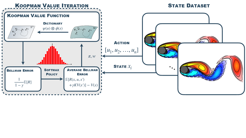
Figure 2: Soft Koopman Value Iteration, a Koopman variant of the widely used value iteration algorithm. In the Koopman value iteration, The set of states $x_{i}$, under a sequence of actions $\{u_{j}\}_{j=1,\ldots,n}$, are lifted onto the vector space to advance the dynamics with the Koopman operator linearly. The action policy is then learned in this new space.

3.1.1 Soft Koopman Value Iteration

The proposed soft Koopman value iteration approach is shown in Fig. 2. In addition to assuming that we have a finite-dimensional approximation of the Koopman operator, we will also assume that the optimal value function $V^{\star}(x)$ can be written as a linear combination of basis functions. In other words, there exists a $w^{\star}\in\mathbb{R}^{d}$, such that $V^{\star}(x)=(w^{\star})^{\top}\phi(x)$. Given a $w\in\mathbb{R}^{d}$, we can express the entropy regularized Bellman error as follows. For any $x$ the Bellman error is:

$$w^{\top}\phi(x)-\min_{\pi:\mathcal{X}\mapsto\Delta(\mathcal{U})}\left[\mathbb{E}_{u\sim\pi(x)}\left[c(x,u)+\alpha\ln\pi(u|x)+w^{\top}K^{u}\phi(x)\right]\right].$$

Thanks to the entropy regularization, given a $w$, we can express the optimal form of $\pi$ as follows:

$$\pi(u|x)=\exp\left(-\left(c(x,u)+w^{\top}K^{u}\phi(x)\right)/\alpha\right)/Z_{x},$$ (23)

where $Z_{x}$ is the normalizing constant that only depends on $x$ and makes $\pi(\cdot|x)$ a proper probability distribution (i.e., probabilities sum to 1). Note that $\pi$ depends on $w$.

Converting this into an iterative procedure to find the value function weights, $w^{\prime}$, in terms of the previous weights, $w$, the average Bellman error (ABE) over the data can be expressed as:

$$\min_{w^{\prime}:\|w\|_{2}\leq W}\frac{1}{N}\sum_{i=1}^{N}\left(w^{\prime\top}\phi(x)-\min_{\pi(\cdot|x)}\left[\mathbb{E}_{u\sim\pi(x)}\left[c(x,u)+\alpha\ln\pi(u|x)+w^{\top}K^{u}\phi(x)\right]\right]\right)^{2}.$$ (24)

This is a canonical ordinary least squares (OLS) problem that can be solved explicitly for $w^{\prime}$. We repeat this procedure until the ABE is small or until convergence. Unfortunately, given finite data, it is possible for a suboptimal value function to satisfy the Bellman equation exactly [94]. Thus, we must be careful when using the Bellman error as a training objective for RL agents.

Algorithm 1 Learning Optimal Policy via Average Bellman Error (ABE) Minimization

0:  Confidence parameter $\epsilon$, reward function or reward function approximator $r$, and feature maps on the state $\phi:\mathcal{X}\to\mathbb{R}^{d_{x}}$ and the control $\psi:\mathcal{U}\to\mathbb{R}^{d_{u}}$. 2 datasets $\mathcal{D}_{x}$ and $\mathcal{D}_{x}$ that store a comprehensive set of possible states of the environment. Initialize $w_{0}$ as desired.

1:  Let $ABE$ denote the objective of the minimization problem (24).

2:  Let $\pi_{0}^{*}(u|x)$ be the optimal policy given in (23) evaluated at $w_{0}$

3:  $ABE(w_{i},\pi_{i})=ABE(w_{0},\pi_{0}^{*})$

4:  while $ABE(w_{i},\pi_{i})>\epsilon$ do

5:     Sample $x_{i}\sim_{iid}\mathcal{D}_{x}$

6:     Compute costs, log probabilities, and value function outputs of all $(x_{i},u)$ pairs for all $u\in\mathcal{D}_{u}$

7:     $w_{i+1}=$ solution to Equation (24)

8:     $w_{i+1}\mapsto\pi_{i+1}^{*}(u|x)$

9:     $ABE(w_{i},\pi_{i})=ABE(w_{i+1},\pi_{i+1}^{*}(u|x))$

10:  end while

3.1.2 Soft Actor Koopman-Critic

Here, we outline how we modify the Soft Actor-Critic framework [53] to restrict the search space by incorporating information from the Koopman operator. An illustration of the Soft Actor Koopman-Critic can be seen in Fig. 1. Using the same loss functions and similar notation to that of the SAC paper [53], we first specify the soft value function loss:

$$J_{V}(w)=\mathbb{E}_{x\sim\mathcal{D}}\left[\frac{1}{2}\left(V_{w}(x)-\mathbb{E}_{u\sim\pi_{\phi}}\left[Q_{\theta}(x,u)-\alpha\ln\pi_{\nu}(u|x)\right]\right)^{2}\right].$$ (25)

The additional specification that is imposed in the Koopman RL framework would be a restriction around the specifications of $V_{w}(x)$ and $Q_{\theta}(x,u)$:

$$V_{w}(x) =w^{T}\phi(x),$$ (26)

where $w$ is a vector of coefficients for the dictionary functions.

Next, we show how the loss function for the quality function $Q$ changes:

$$J_{Q}(\theta)=\mathbb{E}_{(x,u)\sim\mathcal{D}}\left[\frac{1}{2}\left(Q_{\theta}(x,u)-\widehat{Q}(x,u)\right)\right],$$ (27)

where the target $Q$-function incorporates the Koopman operator and is defined as:

$$\widehat{Q}(x,u) =r(x,u)+\gamma\mathbb{E}_{x\sim p(\cdot|x,u)}\left[V_{\bar{w}}(x)\right]$$

$$=r(x,u)+\gamma\bar{w}^{T}K^{u}\phi(x),$$ (28)

and where $\mathcal{K}$ represents the infinite-dimensional Koopman for a fixed action $u$ and $K^{u}$ represents the finite-dimensional approximation of the Koopman operator in the state-dictionary space.

Finally, the loss function for the policy does not change and is given by:

$$J_{\pi}(\nu)=\mathbb{E}_{x\sim\mathcal{D}}\left[D_{KL}\left(\pi_{\nu}(\cdot|x)\left\|\frac{\exp(Q_{\theta}(x,\cdot))}{Z_{\theta}(x)}\right)\right].\right.$$ (29)

After these adjustments, the algorithm remains the same as in SAC and is given by Algorithm 2.

Algorithm 2 Soft Actor Koopman-Critic

0:  Initial parameter vectors $\nu$, $w$, $\theta$, $\bar{w}$

1:  for each iteration do

2:     for each environment step do

3:        $u{\sim}\pi_{\nu}(u|x)$

4:        $x^{\prime}\sim p(x^{\prime}|x,u)$

5:        $\mathcal{D}\leftarrow{\mathcal{D}\cup\{(x,u,r(x,u),x^{\prime}\}}$

6:     end for

7:     for each gradient step do

8:        $w\leftarrow{w-\lambda_{V}\hat{\nabla}_{\nu}J_{V}(w)}$

9:        $\theta_{i}\leftarrow{\theta_{i}-\lambda_{Q}\hat{\nabla}_{\theta_{i}}J_{Q(\theta_{i})}\text{ for }i\in\{1,2\}}$

10:        $\nu\leftarrow{\nu-\lambda_{\pi}\hat{\nabla}_{\nu}J_{\pi}(\nu)}$

11:        $\bar{w}\leftarrow{\tau w+(1-\tau)\bar{w}}$

12:     end for

13:  end for

3.2 Koopman Tensor Formulation of Controlled Dynamics

We now focus on how to advance the basis functions via the Koopman operator, given the current state and action. That is, we would like to find the mapping $(x,u)\mapsto\phi(x^{\prime})$. We also impose that the dictionary functions approximately span a finite-dimensional Koopman-invariant subspace of the value function for each $u$, so that there exists a matrix $K^{u}\in\mathbb{R}^{d_{x}\times d_{x}}$ such that $K^{u}\phi(x)=\phi(x^{\prime})$.

The goal is to construct the Koopman matrix $K^{u}$ for every action $u\in\mathcal{U}$ given state and action trajectory data and a state dictionary space $\phi$. To do so, we take an approach similar to that described in SINDYc [64, 65] where a dictionary space on states and actions is used to predict the next state, that is $\Theta(x,u)\mapsto x^{\prime}$. There are 2 important differences in our approach. First, we are not trying to predict the next state $x^{\prime}$, but rather the next dictionary function value $\phi(x^{\prime})$. Second, to respect the fact that the state dictionary space spans a Koopman invariant subspace for every $u$, it must be that the state-action dictionary is separable in state and action. Modeling the state-action dictionary space as multiplicatively separable as $\psi(u)\otimes\phi(x)$ and then further assuming that there exists a linear mapping $\psi(u)\otimes\phi(x)\mapsto\phi(x^{\prime})$ allows us to construct a Koopman matrix $K^{u}$ for every action $u$. In what follows, we formally describe how constructing a tensor from the linear operator $\psi\otimes\phi\mapsto\phi$ allows us to calculate the matrix $K^{u}$ for any given u.

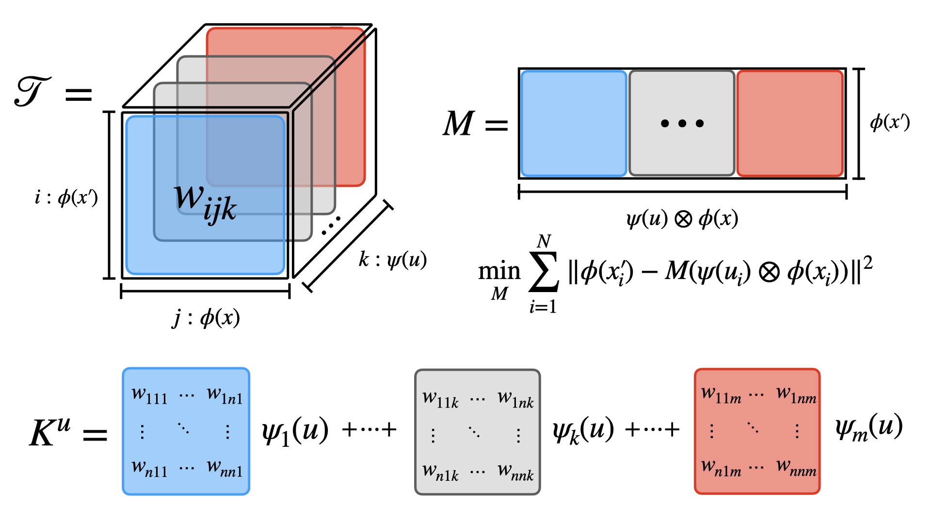
Figure 3: Construction of action-dependent Koopman operators $K^{u}$ from the Koopman tensor $\mathscr{T}_{K}$. Colors match along the $k$ index (depth of tensor box). Each of the matrix slices is then weighted according to the $\psi$ dictionary elements to construct the control-dependent Koopman operator $K^{u}$.

Algorithm 3 Koopman Tensor Estimation

0:  State feature map $\phi:\mathcal{X}\to\mathbb{R}^{d_{x}}$, control feature map $\psi:\mathcal{U}\to\mathbb{R}^{d_{u}}$, and a sample $\{(x_{i},u_{i})\}_{i=0}^{N}$ 

1:  Solve for $\widehat{M}$ as in Equation 30

2:  Convert $M$ into $\mathscr{T}_{K}$ tensor using Fortran-style reshaping

Denote $\phi:\mathcal{X}\mapsto\mathbb{R}^{d_{x}}$ as the feature mapping for the state (each coordinate of $\phi$ is an observable function), and $\psi:\mathcal{U}\mapsto\mathbb{R}^{d_{u}}$ as the feature mapping for control actions. We seek a finite-dimensional approximation of the Koopman operator $\mathcal{K}^{u}$ for all $u\in\mathcal{U}$. Denote $\mathscr{T}_{K}\in\mathbb{R}^{d_{x}\times d_{x}\times d_{u}}$ as a 3D tensor as shown in Fig. 3. For any $u$, define $K^{u}\in\mathbb{R}^{d_{x}\times d_{x}}$ as follows: $K^{u}[i,j]=\sum_{z=1}^{d}\mathscr{T}_{K}(i,j,z)\psi(u)[z]$. Namely, $K^{u}$ is the result of the tensor vector product along the third dimension of $\mathscr{T}_{K}$ and $K^{u}$ serves as the finite-dimensional approximation of Koopman operator $\mathcal{K}^{u}$. We learn $\mathscr{T}_{K}$ to minimize the error in advancing the basis functions $\phi$, averaged over the data:

$$\min_{\mathscr{T}_{K}}\sum_{i=1}^{N}\left\|K^{u_{i}}\phi(x_{i})-\phi(x_{i}^{\prime})\right\|^{2}.$$

We can rewrite the above objective so it becomes a regular multi-variate linear regression problem, rearrange $\mathscr{T}_{K}$ as a 2-dimensional matrix in $\mathbb{R}^{d_{x}\times d_{x}\cdot d_{u}}$. Denote $M\in\mathbb{R}^{d_{x}\times d_{x}\cdot d_{u}}$, where $M[i,:]\in\mathbb{R}^{d_{x}\cdot d_{u}}$ is the vector from stacking the columns of the 2D matrix $\mathscr{T}_{K}[i,:,:]$, as shown in Fig. 3. Denote $\psi(u)\otimes\phi(x)\in\mathbb{R}^{d_{x}\cdot d_{u}}$ as the Kronecker product. Thus we have:

$$K^{u}\phi(x)=M(\psi(u)\otimes\phi(x)).$$

Therefore, the optimization problem becomes a regular linear regression:

$$\min_{M}\sum_{i=1}^{N}\left\|M\left(\psi(u)\otimes\phi(x_{i})\right)-\phi(x_{i}^{\prime})\right\|^{2}.$$ (30)

Once we compute $M$, we can convert back to a standard Koopman operator for any $u\in\mathcal{U}$ by reshaping $M$ back to the 3D tensor $\mathscr{T}_{K}$. Then the $d_{x}\times d_{x}$ finite dimensional Koopman operator approximation is again $K^{u}$ for any $u\in\mathcal{U}$ as seen in the summation in Fig. 3.

Note that the above formulation also works for a discrete control set $\mathcal{U}$, which could improve sample efficiency as opposed to learning independent Koopman operators one for each discrete control.

3.3 Koopman with Control from a Policy Perspective

There have been several attempts to develop extensions of Koopman operator theory to incorporate control [49, 92, 51]. Here, we develop some simple results that enable transformations between different Koopman with control representations. Figure 4 shows a basic schematic that will be useful for the discussion. Note that this section only deals with deterministic systems, although the arguments may be readily extended to the stochastic setting.

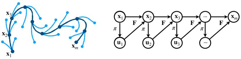
Figure 4: Schematic of Koopman with control. (left) A nominal trajectory is shown for a given policy $\pi$, with alternative branches for different control actions. (right) A diagram showing the state and control sequences, as they relate to the policy $\pi$ and dynamics ${F}$.

If the control action $u$ is a constant for the entire trajectory, then the controlled system may be viewed as an autonomous system parameterized by $u$, and we may define ${F}^{u}$ and $\mathcal{K}^{u}$ as:

$$x^{\prime} ={F}(x,u):={F}^{u}(x)$$ (31a)

$$g(x^{\prime}) =g({F}^{u}(x)):=\mathcal{K}^{u}g(x).$$ (31b)

Similarly, for a given fixed policy $\pi(u,x)$, we may define the autonomous systems ${F}^{\pi}$ and $\mathcal{K}^{\pi}$ as:

$$x^{\prime} ={F}(x,\pi(x)):={F}^{\pi}(x)$$ (32a)

$$g(x^{\prime}) =g({F}^{\pi}(x)):=\mathcal{K}^{\pi}g(x).$$ (32b)

In both cases, for a fixed control $u$ or a fixed control law $u=\pi(x)$, the dynamics may be viewed as autonomous and standard Koopman operator techniques may be used to approximate $\mathcal{K}^{u}$ and $\mathcal{K}^{\pi}$.

If $\pi(x)=u$ at a specific point $x$, then the following

$$g(x^{\prime})=\mathcal{K}^{u}(x)$$ (33)

and

$$g(x^{\prime})=\mathcal{K}^{\pi}(x)$$ (34)

are equivalent at the point $x$, although they are not necessarily equivalent at other points. This has implications for representations in a basis $\{\phi_{j}(x)\}_{j=1}^{n}$. If $g(x)={w}^{T}\bm{\phi}(x)$ then

$$\mathcal{K}^{u}g(x)={w}^{\top}{K}^{u}\phi(x)$$ (35)

and

$$\mathcal{K}^{\pi}g(x)={w}^{\top}{K}^{\pi}\phi(x)$$ (36)

must be equal at the point $x$. Thus, the following must be true at $x$:

$${w}^{\top}{K}^{u}\phi(x)={w}^{\top}{K}^{\pi}\phi(x).$$ (37)

4 Evaluation

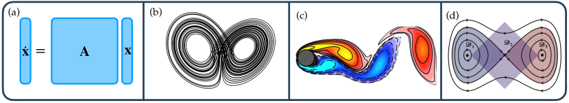
Figure 5: Four benchmark problems investigated: (a) simple linear system; (b) Lorenz 1963 model; (c) incompressible fluid flow past a cylinder at Reynolds number 100; and (d) double-well potential with non-isotropic stochastic forcing.

To evaluate our KARL algorithms, we implemented four benchmark environments widely used in the classical dynamics and control literature. In addition, we implemented classic control baselines to compare our algorithms to. For this purpose, we implemented the linear quadratic regulator and utilized the SAC implementation of CleanRL [95] which are both contained in the same codebase as our SKVI and SAKC algorithms. We will first detail the environments before going into the implementation of the classic control algorithm baselines and the design of the evaluation experiments.

4.1 Environments and Cost Function

Linear System.

This environment is a simple, general form of a controlled, linear system. The linear quadratic regulator (LQR) is optimal for this system. The discrete-time dynamics for the linear system are given by:

$$F(x,u)=Ax+Bu,$$ (38)

where $A$ and $B$ are matrices.

Fluid Flow.

This environment approximates the fluid flow past a cylinder, for which we build on the reduced-order model developed by Noack et al. [96] used for the testing of Koopman modeling algorithms such as in Lusch et al. [58] previously. The continuous-time dynamics are given by:

$${f}(x,u)=\begin{bmatrix}\mu x_{0}-\omega x_{1}+Ax_{0}x_{2}\\ \omega x_{0}+\mu x_{1}+Ax_{1}x_{2}+u\\ -\lambda(x_{2}-x_{0}^{2}-x_{1}^{2})\end{bmatrix},$$ (39)

where $\mu=0.1$, $\omega=1.0$, $A=-0.1$, and $\lambda=1$. The states $x_{0}$ and $x_{1}$ represent the most energetic proper orthogonal decomposition modes for the flow, and the third state $x_{2}$ represents the shift mode, used for capturing the relevant transients.

Lorenz 1963.

This is a standard canonical chaotic benchmark dynamical system often used to evaluate Koopman-based approaches due to its continuous eigenvalue spectrum [77]. The continuous-time dynamics are governed by the following system of equations:

$${f}(x,u)=\begin{bmatrix}\sigma(x_{1}-x_{0})+u\\ (\rho-x_{2})x_{0}-x_{1}\\ x_{0}x_{1}-\beta x_{2}\end{bmatrix},$$ (40)

where $\sigma=10$, $\rho=28$, and $\beta=\frac{8}{3}$.

Stochastic Double Well.

In this environment, we consider the stochastically forced particle in a double well potential, governed by the following dynamics:

$${f}(x,u)=\begin{bmatrix}4x_{0}-4x_{0}^{3}+u\\ -2x_{1}+u\end{bmatrix}+\begin{bmatrix}0.7&x_{0}\\ 0&0.5\end{bmatrix}\begin{bmatrix}v_{0}\sim\mathcal{N}(0,1)\\ v_{1}\sim\mathcal{N}(0,1)\end{bmatrix}.$$ (41)

Cost Function.

All policies use the LQR cost function for each system defined by:

$$c(x,u)=(x-x_{e})^{\top}Q(x-x_{e})+u^{\top}Ru$$ (42)

where $x_{e}$ is the reference point we wish to stabilize, and $Q$ and $R$ are positive-semi-definite matrices. For all environments except Lorenz, $x_{e}$ is the origin and in Lorenz, it is the critical point

$$x_{e}=\begin{bmatrix}x_{1e}\\ x_{2e}\\ x_{3e}\end{bmatrix}=\begin{bmatrix}\sqrt{\beta(\rho-1)}\\ \sqrt{\beta(\rho-1)}\\ \rho-1\end{bmatrix}$$ (43)

where the parameters are $\sigma=10$, $\rho=28$, $\beta=8/3$ and the simulation time step is $dt=0.01$.

4.2 Baseline Control and Learning Algoritms

Linear Quadratic Regulator.

LQR is implemented using the Python Control Systems Library  on top of our CleanRL-based code. The dlqr function is used for the linear system, and the lqr function is used for the other three systems. The linear system is the only system that has inherent ${A}$ and ${B}$ matrices as in ${A}x+{B}u$. To recover usable ${A}$ and ${B}$ matrices for the other three systems, we linearize the system dynamics around the fixed reference point we are attempting to stabilize. For computing cost, Q and R are identity matrices for all systems except in Lorenz where the R matrix is an identity matrix multiplied by $0.001$ to incentivize action from the agent.

Soft Actor-Critic Baselines.

We have two reinforcement learning baselines that are different implementations of the Soft Actor-Critic model. The first is from the original paper [53] and explicitly makes use of function approximators for both Q and V. We denote this algorithm by SAC (V). The algorithm is exactly as shown in Algorithm 2 except that the value function $V_{w}$ is approximated by a neural network rather than a linear combination of the dictionary functions. In this implementation, there are four neural networks: $V_{w}$, $Q_{\theta_{1}}$, $Q_{\theta_{2}}$, and $\pi_{\nu}$ with parameter vectors $w,\theta_{1},\theta_{2}$ and $\nu$, respectively. The following implementation details apply:

• The policy $\pi_{\nu}$ is assumed to be the normal density function with mean and standard deviation being represented by the policy neural network.

• All networks are fully connected feed-forward networks of 1 hidden layer with 256 neurons, each with ReLU activation functions.

• The standard deviation is ”squashed” with a $\tanh$ transformation, and a convex combination transformation that maintains the log standard deviation of the policy between $2$, and $-5$.

• The learning rate of both the Q and V networks are taken to be $1$e-$3$, whereas the policy network learning rate is taken to be $3$e-$4$.

• The replay pool (or buffer) is of max size $1$e$6$, and is initialized with $5000$ interactions in the environment following the initial policy. After $5000$ steps, the policy starts to update and after $1$e$6$ total steps, a FIFO replacement scheme is followed for updating the replay buffer.

Finally, we also use the standard implementation of SAC from [54] as a baseline, which is a reference implementation of the CleanRL library. This implementation removes the V-network and the V-target network is replaced with a Q-target network. All other implementation details remain the same as above and the full algorithm 4 is included below for completeness.

Algorithm 4 Soft Actor-Critic (Q)

0:  Initial parameters $\theta_{1},\theta_{2},\nu$

1:  Initialize target Q-network weights $\overline{\theta}_{1}\leftarrow\theta_{1},\overline{\theta}_{2}\leftarrow\theta_{2}$

2:  Initialize a replay pool $\mathcal{D}$ by interacting with the enviroment with the initial policy

3:  for $t\in\text{iterations}$ do

4:     for $s\in\text{environment steps}$ do

5:        $a\sim\pi_{\nu}(a|x)$ {Sample action}

6:        $(x^{\prime},r(x,a))\sim p(x^{\prime}|x,a)${Sample transition}

7:        Store transition $(x,a,r(x,a),x^{\prime})$ in $\mathcal{D}$

8:        $\mathcal{D}\leftarrow{\mathcal{D}\cup\{(x,u,r(x,u),x^{\prime}\}}$

9:     end for

10:     for $j\in\text{gradient steps}$ do

11:        $\theta_{i}\leftarrow\theta_{i}-\lambda_{Q}\nabla_{\theta_{i}}J_{Q}(\theta_{i})$ for $i\in\{1,2\}$ {Update Q-function parameters}

12:        $\nu\leftarrow\nu-\lambda_{\pi}\nabla_{\nu}J_{\pi}(\nu)$ {Update policy weights}

13:        $\alpha\leftarrow\alpha-\lambda\nabla_{\alpha}J(\alpha)$ {Adjust temperature}

14:        $\overline{\theta}_{i}\leftarrow\tau\theta_{i}+(1-\tau)\overline{\theta}_{i}$ for $i\in\{1,2\}$ {Update target network weights}

15:     end for

16:  end for

16:  Optimized parameters $\theta_{1},\theta_{2},\nu$

4.3 KARL Algorithm Implementation Specifics

Construction of the Koopman Tensor.

The Koopman tensor, outlined in section 3.2 and figure 3, and its action-dependent feature space Koopman operator $K^{u}$ are used in both the SKVI, and SAKC algorithm below. The dataset from which the Koopman tensor is constructed is comprised of $3$e$+4$ interactions with the environment under a random agent; this agent chooses actions uniformly at random with bounds dependent on the specific environment. The bounds were chosen according to the minimum and maximum actions taken by an LQR policy.

Discrete Soft Koopman Value Iteration.

DSKVI was implemented with a manual calculation of the average Bellman error given a set of system states, and the extraction of the softmax policy. For the discrete value iteration, we use the same dataset used for the construction of the Koopman tensor. For our discretized action space, we use the min, and max action in the system’s range with the number of actions evenly splitting the range. After the value iteration policy is trained, it is run against the same initial conditions as shown in Fig. 6.

Soft Actor Koopman-Critic.

SAKC follows Algorithm 2 with the cost and target functions as in section 3.1.2. This algorithm mirrors all specification details of SAC (V) with the exception of how the value function and its continuation value are represented. Specifically, as discussed in section 3.1.2, the value function $V_{w}(x)$ is approximated in the feature space as $V_{w}(x)=w^{T}\phi(x)$ and the continuation value is represented with the Koopman operator in the state feature space as $\mathbb{E}_{x\sim p(\cdot|x,u)}\left[V_{w}(x)\right]=w^{T}K^{u}\phi(x)$. The learning rate on the parameter $w$ is set to $1$e-$3$.

4.4 Design of Evaluation

We run a set of four experiments to measure the performance characteristics of the KARL algorithms with respect to episodic returns, comparison to baselines, interpretability, and sensitivity to the chosen dictionary space. To examine the performance of the two proposed KARL variants, we measure the episodic return on all four environments, averaging over $50$ seeds. These are compared to LQR, CleanRL’s implementation of the $Q$ function-based SAC algorithm, and the $V$ function-based SAC algorithm. We further evaluate the performance of all five tested algorithms for their average episodic return across $100$ episodes on their respective saved policies across all four environments.

To inspect the interpretability of the KARL policies, we extract a set of three simplified value functions, and evaluate their policy rollout across $50000$ steps at $5$ random seeds.

The influence of hyperparameter choices on KARL-based algorithms is analyzed by performing extensive ablation analyses for both the SKVI, and the SAKC. In the case of SKVI, we inspect the sensitivity to the choice of the batch size by varying the batch size between $2^{13}$, and $2^{14}+2^{13}$ in increments of $2^{12}$. We further test the sensitivity to the amount of compute afforded for the construction of the Koopman tensor by varying the number of actions the policy can sample from, between $61$, and $141$ in increments of $20$, while simultaneously varying the number of epochs the model is trained over between $90$, and $190$ in increments of $20$. In the case of SAKC, we analyze its sensitivity to the order of monomials used for the construction of the Koopman tensor’s state and action dictionary spaces. We vary the order of monomials used for the construction of the dictionaries between $1$, and $4$ for both states and actions simultaneously on all four environments. To discern the sensitivity of SAKC to the amount of compute used to construct the Koopman tensor, the number of random interactions the Koopman tensor is afforded in its construction is varied between $6000$, and $70000$ by varying the number of steps per sampled path between $100$, and $500$ in increments of $100$, and the number of sampled paths between $60$ and $140$ and then computing the mean episodic return on all four environments. All ablation analyses are based on a mean of $5$ seeds, where the mean episodic return of the policies is computed.  

All reinforcement learning algorithms rely on the CleanRL reinforcement learning library [95] to ensure correctness of compared-to baselines, and full reproducibility. Unless stated otherwise, the Koopman tensor algorithm relies on a dictionary space of second-order monomials for both the state space and action space dictionary. The Koopman tensor is trained on $30000$ data snapshots collected by a random agent unless stated otherwise.

All experiments are performed on the University of Washington’s Hyak  cluster environment on a node with the following specifications:

• Rocky Linux 8.5

• 4.18.0

• $2\times$ 26 Core Intel Xeon Gold 6320R 2.10 GHz with hyperthreading disabled

• 1056GB

The code to reproduce all experiments is available in the KoopmanRL repository . All experiments were run entirely on CPU. Datasets for all experiments run in the paper can be found in the KoopmanRL Hugging Face data repository .

5 Results

We first examine the results of the Koopman-assisted reinforcement learning algorithms on the four benchmark environments. The episodic returns of the algorithms on the linear system, the fluid flow, Lorenz, and the double well environment are shown in figure 6. Subsequently, we examine the interpretability of the algorithms, their average return of evaluation rollouts performance, and the ablation analyses of their sensitivities to algorithmic design choices.

5.1 Algorithm Performance on Benchmark Problems

The performance of Soft Actor Koopman-Critic is evaluated on the four environments and compared against the classical control baseline, as well as the reference SAC (Q) and SAC (V) algorithms. We see that on the Linear System, SAKC needs $\approx 5000$ environment steps to properly initialize the Koopman tensor and calibrate its Koopman critic to match the SOTA performance of LQR, the soft Koopman value iteration, and SAC (V). Zooming into the performance of the linear system in figure 7, we see that LQR performs best consistently, with SKVI performing nearly as well. SAKC and SAC (V) closely track each other’s performance, slightly lagging behind the performance of LQR, SKVI, and SAC (Q).

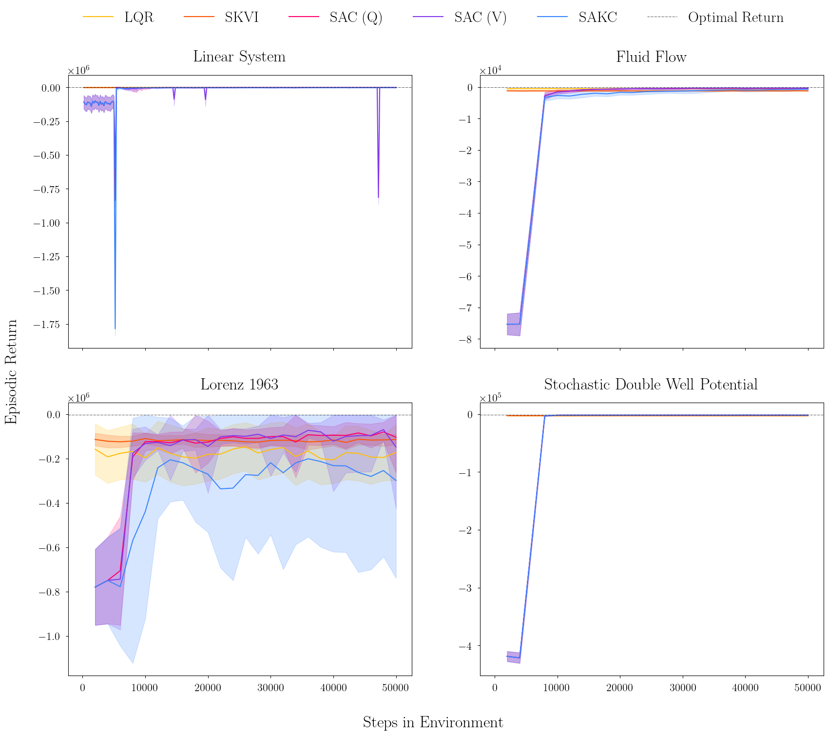
Figure 6: Episodic returns of the evaluation environments for the compared algorithms. We consider the Koopman value iteration, the linear quadratic regulator (LQR), the Q-function-based soft actor-critic (SAC (Q)), the V-function-based soft actor-critic (SAC (V)), and the soft actor Koopman-critic (SAKC). Four environments are being considered, Left Top the Linear System, Right Top Fluid Flow, Left Bottom Lorenz 1963, and Right Bottom the Stochastic Double Well.

On the Fluid Flow environment, this training dynamic is matched, with SAKC and SAC (V) requiring $\approx 5000-8000$ environment steps to explore the environment. Importantly, SAKC reaches SOTA in this more difficult environment. To better inspect the performance differences between the tested algorithms in this more challenging environment, we again provide a zoomed-in excerpt covering $10000$ to $50000$ steps in figure 8. The performance of LQR stays stably at a high level, with it notably outperforming the reinforcement learning algorithms in the low resource setting with $\leq 10000$ steps in the environment. The actor-critic based reinforcement learning algorithms begin to outperform with more steps in the environment. The SAC (Q) and SAC (V) algorithms lead in performance, and SAKC tracks closely behind, showing its need for slightly more interactions with the environment to reach comparably high performance.

On the chaotic Lorenz 1963, the Koopman tensor requires slightly more exploration with $10000$ random environment steps before SAKC is calibrated, and the actor-critic based Koopman architecture fails to meet the performance of the other reinforcement learning algorithms. SKVI performs at the same level as the two soft actor-critic baselines, with stable episodic returns from the beginning with tight standard deviation bounds accompanying it.

On the Stochastic Double Well, we see a fast calibration of SAKC and SAC (V) to quickly match SOTA, while LQR and SKVI are unable to match the performance of the actor-critic architectures in this challenging environment. Zooming in on the performance between $10000$, and $50000$ steps in the environment in figure 8, we see a clear split between the actor-critic design-based architectures and LQR and SKVI. SAKC consistently outperforms the other algorithms, only being occasionally matched by SAC (V).

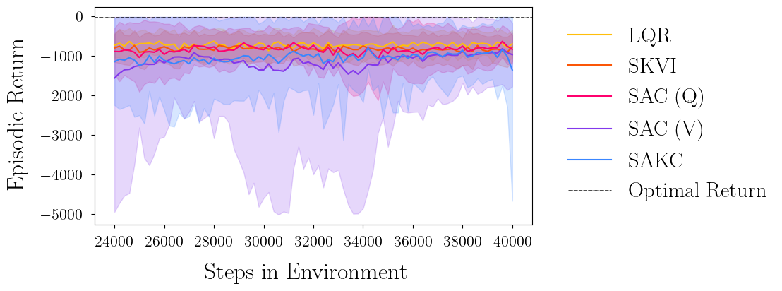
Figure 7: Zoomed in episodic return of the Linear System. The first $24000$, as well as the last $10000$ steps in the environment have been omitted to focus on the performance of the algorithms.

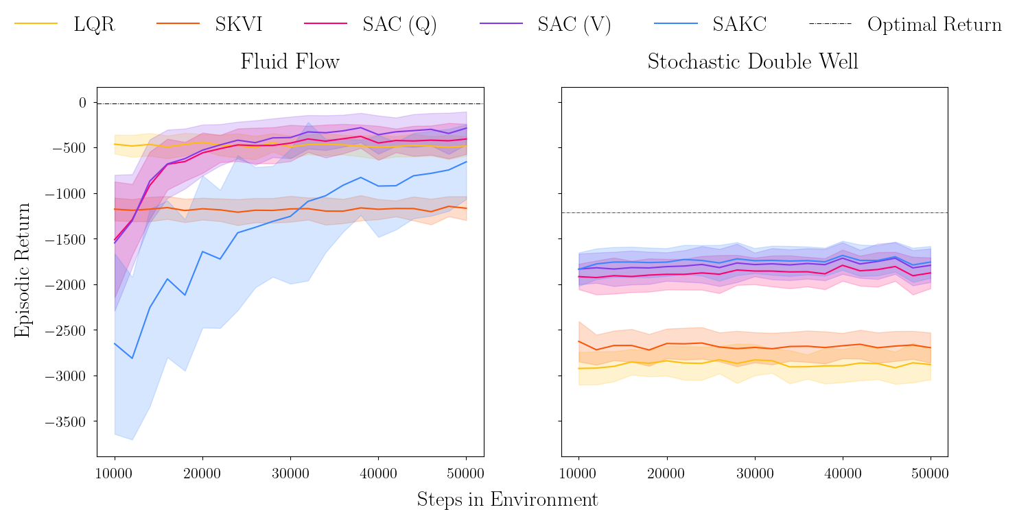
Figure 8: Zoomed in episodic return for the Fluid Flow, and the Stochastic Double Well Potential, where the first $10000$ steps in the environment have not been included due to the large variability of the episodic return during the initial $10000$ steps. The Soft Koopman Value Iteration (SKVI)a shows here that its performance lags behind that of the actor-critic based algorithms. The value-based Soft Actor-Critic (SAC (V)), and the Soft Actor Koopman-Critic (SAKC) closely track each other’s performance, with SAKC having the slightly better performance.

5.2 Interpretability of Koopman Reinforcement Learning

By exploiting KARL’s native interpretability, users can influence the RL policy’s behavior. This is an approach that is not possible with standard opaque optimal value function modeling methods. To demonstrate this, we inspect the fluid flow environment where we leverage the candidate-function space comprised of identifiable component terms and, in turn, the array of coefficients for those terms corresponding to the optimal value function. For this, we elected to limit the dictionary space to order-2 monomials, and then used SKVI to generate the optimal set of coefficients for the 10 terms in the dictionary space, given by

$$V(x) =-333.80+22.59x-8.01y-157.57z+267.93x^{2}$$

$$-80.52xy-27.16xz+173.22y^{2}+6.29yz+149.42z^{2}.$$

By revealing the relative contributions of each term, in contrast to non-interpretable models, KARL supports a more informed approach to tailoring value functions. To this end, we construct a set of more simple value functions with comparable performance by selecting a narrow subset of key variables. Table 1 shows the simpler value functions, and their relative performance of selected sub-optimal value functions following the use of expert-informed sparsification. We focus on a hand-picked subset of more critical features of the environment. For example, our extensive interaction with fluid flow simulations indicated that forcing the $y$ spatial coordinate had more impact than other components. Moreover, experiments demonstrated that policies derived from these expert-tuned value functions, even those heavily reliant on a single term such as $y^{2}$, exhibited near-optimal performance. Thus, expert knowledge, guided by interpretability, identified the importance of simpler, and potentially more generalizable, value functions.

Slightly suboptimal value functions, using fewer terms, still achieve desired levels of performance and hold promise for improved generalizability, as shown in Table 1 and figure 9. Individual terms of the optimal value function stabilize the episodic returns rollouts, furthermore resulting in lower standard deviation bounds with less fluctuation than the sparsified value functions. The ability to fine-tune learned value functions is critical for real-world RL applications, where training data often fails to capture deployment environments, including both dynamics and reward functions. This example case study shows KARL’s ability to enable more interpretability in RL for guiding efforts to simplify and improve model output and to support adaptability to real-world environments with imperfect simulators or unsatisfactory reward functions. By allowing experts to limit dependence on less important terms, KARL promotes value functions focused on more crucial outcome drivers across diverse scenarios, facilitating prospects for more generalizable policies. This aligns with the observation that policies derived from the expert-tuned value functions in Table 1 maintained near-optimal performance.

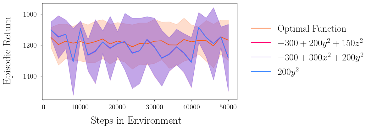
Figure 9: Episodic returns rollouts associated with the soft-max policy of the optimal value function, as well as the 3 extracted value functions. The optimal value function shows stable performance in the rollout with a moderate standard error around it. The 3 extracted value functions all display the same behaviour in the rollout, with most notably a much more significant standard error around the mean, and much less stable behaviour in the rollout.

Value Function $V(x)$	Difference to Optimum	Average Return
$-300+200y^{2}+150z^{2}$	1.81 %	-1170.9836
$-300+300x^{2}+200y^{2}$	1.6 %	-1169.2547
$200y^{2}$	1.83 %	-1171.1773
optimal weights		-1150.1192

Table 1: Extracted Value Functions with Zeroed-out Coefficients on the Fluid Flow environment. The symbolic form of the value function is distilled by reading out the weights of the trained, and cutting away lesser terms.

5.3 Average Cost Comparisons for KARL

Comparing the performance of trained KARL policies, SKVI and SAKC, to the classical LQR and the baseline SAC algorithms, we see nuanced differences between trained policies in Table 2. All results of the table are the mean of 5 policies, trained with different seeds. While 5 seeds begin to encapsulate the stochasticity in RL results, they still allow outliers to have an outsized influence as is the case for the Soft Actor Koopman-Critic, whose performance is impacted by an outlier. If we increase the number of seeds to $50$, then the impact of this outlier will be lessened and we arrive at a mean episodic return of $-315996$ for the Soft Actor Koopman-Critic on Lorenz. For comparability, the number of SAKC in the Lorenz system is based on the mean episodic return of the policies at 5 different seeds.

As expected, LQR does best relative to all methods on the linear system, with the three reinforcement learning algorithms all displaying nearly equally good performance, close to the optimal performance of LQR. In the Fluid Flow system, we see the strong versatility of the SAC-baseline, with the Soft Actor Koopman-Critic likewise performing better than the LQR baseline and the value iteration-based Koopman approach. In the Lorenz system and the stochastic Double Well, we can conclude that the increased complexity is too much for LQR to control. On the Lorenz system, the stable and strong performance of SAC continues, with the value iteration-based Koopman approach close in performance. SAKC performs much less well than SAC on the Lorenz system. The stochastic Double Well environment produces performance of the SAC and the SAKC within the margin of error of each other, with the SAKC outperforming the SAC by a slight margin, and the LQR as well as the SKVI lagging by a significant margin.

Environment	LQR	Soft Actor-Critic	Soft Actor Koopman-Critic	Soft Koopman Value Iteration
Linear System	-690	-775	-809	-746
Fluid Flow	-1610	-307	-697	-1529
Lorenz 1963	-1475235	-104140	-337774	-160555
Stochastic Double Well	-103705	-1795	-1777	-2661

Table 2: Average episodic returns over a 100 episodes rollout to show the comparative average cost incurred by the learned LQR, SAC (V), SAKC, and SKVI policies. Bolded values indicate the lowest average cost, and thus, the best performing controller for each dynamical system. All mean episodic returns are computed across a set of 5 random seeds to account for stochasticity.

Connecting the relative cost measured in table 2 with the average episodic returns of figure 6, we see that when tasked with learning dynamics and converging to an optimal controller in non-linear systems, our new Koopman-assisted reinforcement learning approaches significantly outperformed LQR in non-linear systems as measured by the relative cost, and is within striking distance of the fully-developed, and optimized SAC approach.

5.4 Ablation Analyses

Analyzing some of the hyperparameter choices introduced by the KARL algorithms, we first inspect the influence of these choices on the mean episodic return of the soft Koopman value iteration, before examining the sensitivity to the chosen dictionary space and the sensitivity to the amount of compute afforded to the construction of the Koopman tensor for the performance of the SAKC. The presented ablation studies only present a glimpse into the combinatorial space of potential hyperparameter choices of KARL algorithms, and the resulting algorithm performance.

5.4.1 Soft Koopman Value Iteration

Batch Size.

In table 3, we see that the batch size used to sample from the reply memory has no influence on the performance of the Koopman value iteration algorithm. On all four environments the performance remains unchanged across all $5$ tested batch sizes.

	Batch Size
Environment	8192	12288	16384	20480	24576
Linear System	-827	-832	-835	-814	-824
Fluid Flow	-1167	-1167	1167	1167	1167
Lorenz 1963	-115237	-115142	-115151	115242	-115242
Stochastic Double Well	-2673	-2673	-2673	-2673	-2673

Table 3: Ablation analysis over the batch size with which the Soft Koopman Value Iteration samples from the reply memory. The batch size is varied from $2^{13}$ (8192) to $2^{14}+2^{13}$ (24576) in increments of $2^{12}$ (4096), and the mean episodic return of the training trajectory of all 5 seeds is computed to then be averaged over for the comparison table.

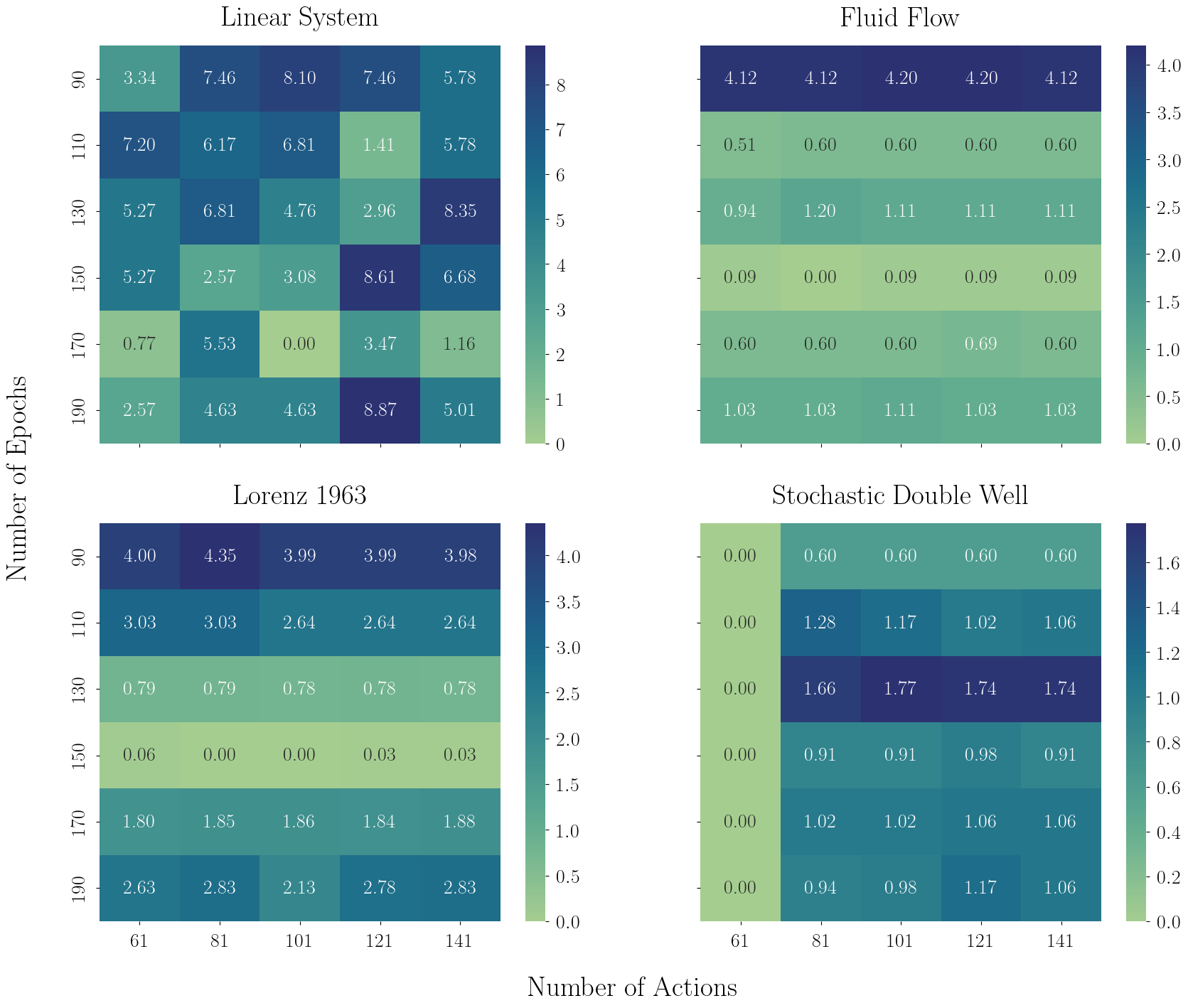
Figure 10: Ablation analysis of the compute afforded to the Soft Koopman Value Iteration (SKVI) algorithm in which the Number of Actions the policy can pick from are varied between $61$, and $141$ in increments of $20$, and the Number of Epochs the model should be trained over are varied between $90$, and $190$ in increments of $20$. Each heatmap is zeroed on the best-performing data point, and then measures the $\%$ difference in mean episodic returns.

Training Budget.

We now inspect the compute budget afforded to the construction of the Koopman tensor in the form of the number of epochs the model is trained over and the number of actions the policy can pick from in figure 10. The amount of compute best afforded to the Koopman tensor construction is highly problem-dependent with all environments having different optimal compute budgets. Each environment has varying complexity, leading to specific compute requirements for the construction of the ideal Koopman tensor. While the fluid flow and Lorenz both show a clear dependence on the number of training epochs, with the best performance at $150$ epochs, and performance degrading in unison with different numbers of epochs. The double well has a clear dependence on the number of actions the policy can pick from, although it shows no sensitivity to the afforded number of training epochs. The linear system, in contrast, does not display any clear trends.

5.4.2 Soft Koopman Actor-Critic

In the SAKC algorithm, the hyperparameters include the compute allocated to the computation of the Koopman tensor, as well as the order of monomials used for the action and state dictionaries.

Choice of the Dictionary Space.

By intuition we would expect the order of monomials for the action and state dictionaries to play an important role for the eventual mean episodic return of the SAKC. This intuition holds for all environments, apart from the stochastic double well potential. Outside of a single bad configuration, the stochastic double well displays no sensitivity to the order of monomials used for the construction of its dictionaries. The linear system, fluid flow, and Lorenz 1963 all exhibit a similar dependency on the order of the monomials of the state dictionary. A monomial order of $2$ is the optimal choice for the linear system and Lorenz system, while the fluid flow benefits from a higher-order family of monomials. All three environments, excluding individual outliers in the linear system and Lorenz, display uniform behaviour in the worsening of the mean episodic return performance as the order of monomials of the state dictionary is varied from the optimal order.

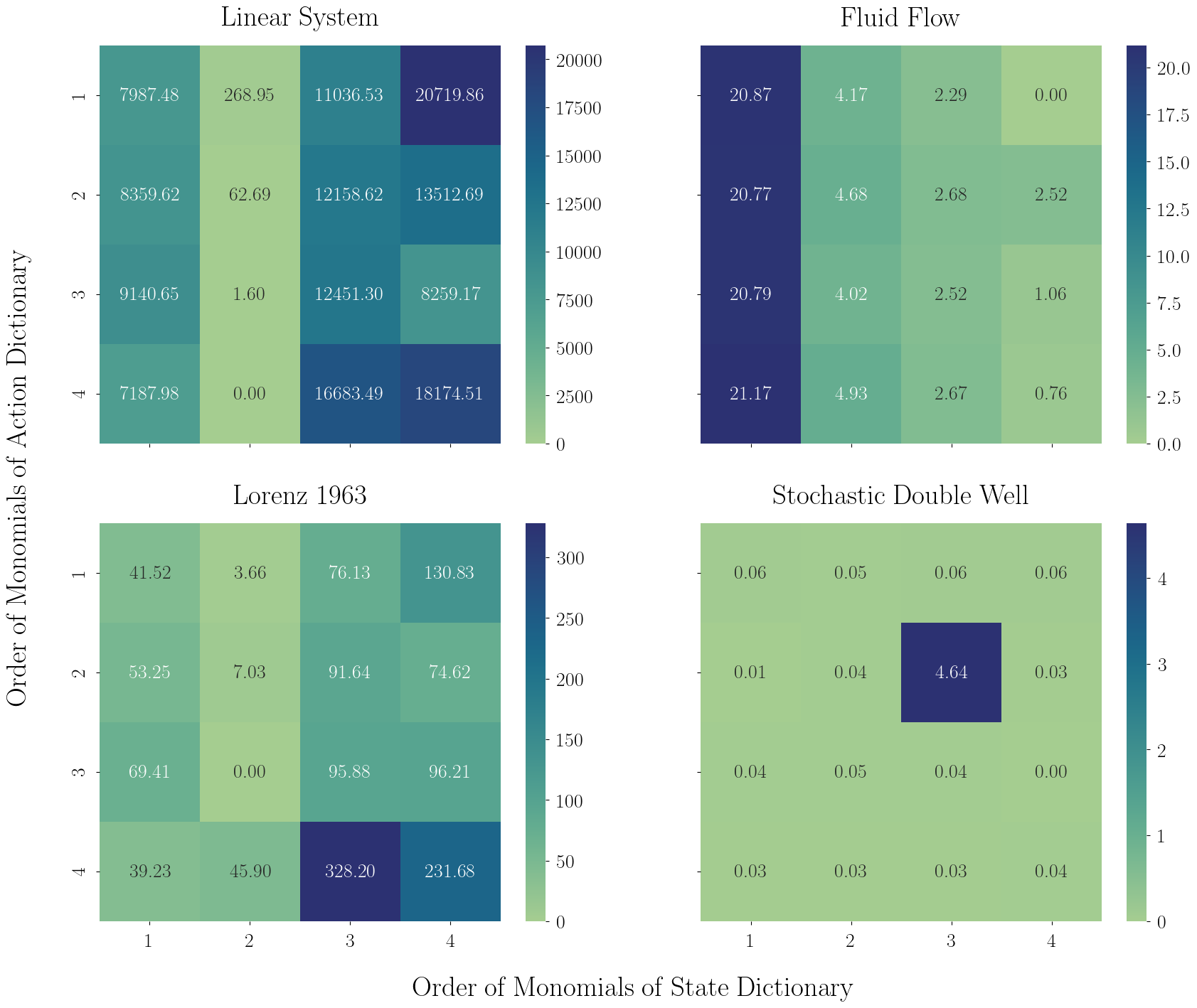
Figure 11: Ablation analysis of the order of monomials used for SAKC. The Order of Monomials of the Action Dictionary is varied from order $1$ to order of $4$, and likewise the Order of Monomials of the State Dictionary are varied from order $1$ to order of $4$. Each heatmap is zeroed on the best-performing value, and then measures the $\%$ difference in mean episodic returns.

Budget for Random Interactions in the Constructions of the Koopman Tensor.

Figure 12 shows the ablation analysis over the amount of compute afforded to the construction of the Koopman tensor for the SAKC algorithm. This analysis reveals little or no trends. We surmise that in the case of SAKC, the amount of compute, reduced to the number of paths the tensor construction samples from, and the number of steps per path, is too reductive as it excludes any interplay with other hyperparameters defining SAKC, which all stay fixed in the current ablation analysis.

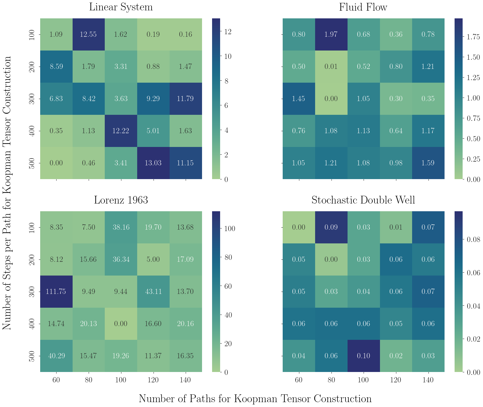
Figure 12: Ablation over the amount of compute allocated to construct the Koopman tensor in the SAKC algorithm. By default, the Koopman tensor uses $30000$ random interactions with the environment sampling from $100$ paths with $300$ interactions each. The number of sampled paths is varied in increments of $20$ between $60$ and $140$, and the steps per path is varied in increments of $100$ from $100$ to $500$. Each heatmap is zeroed on the best-performing data point, and then measures the $\%$ difference in mean episodic returns.

6 Limitations and Future Work

While Koopman-assisted reinforcement learning holds great promise, it faces in its current form a number of limitations, which are the subject of future work. We first note in subsection 6.1 KARL’s crucial dependence on the specification of the dictionary space, and how this aspect of KARL can be extended by considering dictionary spaces paired with sparsification methods. Another inherent constraint of KARL is the current offline, sampling-reliant construction of the Koopman tensor, and thus the action-dependent Koopman operator in the feature space. In subsection 6.2 we outline how this could potentially be addressed with an online, recursive algorithm. Next, KARL is currently limited to discrete-time environments/dynamical systems, and its potential extension to continuous-time systems is discussed in subsection 6.3. Finally, SKVI currently relies on a discretization of the action space for which we briefly discuss the limitations as well as an approach we are developing to allow for the more robust continuous action setting.

6.1 Dictionary Dependence and Discovery

The Koopman approach as outlined above, and further explored in the ablation analysis in subsection 5.4, has a crucial dependence on the correct choice of dictionary space. This dictionary space must both characterize the value function and the dynamic evolution of the value function. Specifically, we require that different linear combinations of the elements of the vector $\phi(x)$ can approximate $V(x)$ and $V(x^{\prime})$ well. There are, however, a number of methods that can be incorporated to help relax the specification of a correct dictionary space. First, to address the problem of finding the Koopman tensor, we recall the regression problem (30). As this is a standard regression problem, it lends itself well to traditional regularization methods such as ridge regression, LASSO regression, or the sequential thresholding methods used in SINDy [64]. Second, to address the problem of finding the representation of the value function at the current state, we can again utilize a large dictionary space while leveraging the aforementioned regression sparsification methods. In particular, the regression problems we face for the problem of fitting the contemporaneous value function in our KARL algorithms are (24) and (25). Again each of these can be treated as a traditional least squares regression problem and admit the use of traditional regularization methods, such as a sparsification.

6.2 Online Learning of the Koopman Tensor

One concern around the construction of the Koopman tensor is its reliance on a sufficiently rich set of static training data. This is problematic in online settings. With this in mind, building on the recursive EDMD (rEDMD) algorithm developed by [97], we suggest an adapted online approach in algorithm 5 to calculate the Koopman tensor, which we call recursive Koopman tensor discovery (rKTD). Testing this approach is the subject of future work.

Algorithm 5 rKTD: Recursive Koopman Tensor Discovery

0:  Incoming data point tuple $(\mathbf{x}_{n},\mathbf{u}_{n},\mathbf{y}_{n})$. Initialize $\upsilon_{0}\leftarrow\delta\textit{I}_{d_{x}d_{u}}$ and $z_{0}\leftarrow 0_{d_{x}\times d_{x}d_{u}}$. $\delta$ should be altered to best fit the specific training problem. $\textit{I}_{d_{x}d_{u}}$ is the $d_{x}d_{u}\times d_{x}d_{u}$ identity matrix. $0_{d_{x}\times d_{x}d_{u}}$ is the $d_{x}\times(d_{x}d_{u})$ zero matrix. Let $\bf\Psi\otimes\Phi$ denote the matrix $[\psi(u_{1})\otimes\phi(x_{1}),\cdots,\psi(u_{n-1})\otimes\phi(x_{n-1})]$ and $\bf\Phi^{\prime}$ be $[\phi(y_{1}),\cdots,\phi(y_{n-1})]$.

1:  Add a new entry to $\bf\Psi\otimes\Phi$ by applying the dictionary functions $\psi\otimes\phi$ to the data point $(\mathbf{x}_{n},\mathbf{u}_{n})$

2:  Add a new entry to $\bf\Phi^{\prime}$ by applying the dictionary functions $\phi$ to the data point $(\mathbf{y}_{n})$

3:  Calculate components of $M_{n}$:

$$z_{n} \leftarrow z_{n-1}+{\bf\Phi^{\prime}}({\bf\Psi\otimes\Phi})^{\top}$$

$$\upsilon_{n}^{-1} \leftarrow\upsilon_{n-1}^{-1}-\frac{\upsilon_{n-1}^{-1}({\bf\Psi\otimes\Phi})({\bf\Psi\otimes\Phi})^{\top}\upsilon_{n-1}^{-1}}{1+({\bf\Psi\otimes\Phi})^{\top}\upsilon_{n-1}^{-1}({\bf\Psi\otimes\Phi)}}$$

4:  $M_{n}=z_{n}v_{n}^{-1}$

5:  return  $M_{n}$

6.3 Continuous-Time Settings: Koopman Generator Approach

Here we recall a useful object for continuous time stochastic processes, the generator of the Koopman operator $\mathcal{L}$. This operator is the time derivative of the Koopman operator evaluated at time $t=0$ for the time homogenous case. The analogous object in discrete time is the transition matrix of $\tilde{X}$.

First, we represent the dynamics of the stochastic process as a stochastic differential equation (SDE) which we will assume is continuous itself, i.e., has no jumps:

$$\text{d}X_{t} =\mu_{x}(X_{t},U_{t})\text{d}t+\sigma_{x}(X_{t},U_{t})\text{d}W_{t}$$ (44a)

$$\text{d}U_{t} =\mu_{u}(X_{t})\text{d}t+\sigma_{u}(X_{t})\text{d}W_{t}.$$ (44b)

Here, $\mu_{x}:\mathbb{X}\times\mathbb{U}\to\mathbb{R}^{n}$ and $\mu_{u}:\mathbb{X}\to\mathbb{R}^{m}$ are the drift terms and $\sigma_{x}:\mathbb{X}\times\mathbb{U}\to\mathbb{R}^{n\times d}$ and $\sigma_{u}:\mathbb{X}\to\mathbb{R}^{m\times d}$ are the diffusion terms, for the state and control, respectively. Finally, $W_{t}$ is a $d$-dimensional Wiener process.

Given a twice continuously differentiable function $f$, it can be shown using Itô’s lemma that the infinitesimal generator of the Koopman operator is characterized by

$$\mathcal{L}^{u}f=\mu_{x}\cdot\nabla_{x}f+\frac{1}{2}a_{x}:\nabla^{2}_{x}f$$ (45)

where $a_{x}={\sigma_{x}}{\sigma_{x}}^{\top}$, $\nabla^{2}_{x}$ denotes the Hessian, and $:$ denotes the double dot product. In this setting the function $k(t,x)=\mathcal{K}_{t}f(x)$ satisfies the second-order partial differential equation $\frac{\partial k}{\partial t}=\mathcal{L}k$, which is called the Kolmogorov backward equation. See [48] for more details. Adapting tools from [48] we can find the Koopman generator tensor by solving the following least squares problem

$$\min_{L\in\mathbb{R}^{d_{x}\times(d_{x}d_{u})}}\sum_{i=1}^{N}\left\|L(\psi(u_{i})\otimes\phi(x_{i}))-\widehat{\mathcal{L}}^{u_{i}}\phi(x_{i})\right\|^{2}$$ (46)

where

$$\widehat{\mathcal{L}}^{u_{i}}\phi=\hat{\mu}_{x}\cdot\nabla_{x}\phi+\frac{1}{2}\hat{a}_{x}:\nabla^{2}_{x}\phi$$ (47)

with

$$\hat{\mu}_{x} :=\frac{\Delta x_{i}}{\Delta_{t}}=\frac{x_{i+1}-x_{i}}{t_{i+1}-t_{i}}$$ (48a)

$$\hat{a}_{x} :=\frac{(\Delta x_{i})(\Delta x_{i})^{\top}}{\Delta_{t}}=\frac{(x_{i+1}-x_{i})(x_{i+1}-x_{i})^{\top}}{(t_{i+1}-t_{i})}$$ (48b)

and $L\in\mathbb{R}^{d_{x}\times(d_{x}d_{u})}$ is the flattened Koopman generator tensor where $d_{x}$ and $d_{u}$ are the dimensions of the state and action feature map dimensions, respectively. As with the discrete-time Koopman tensor, once we compute $L$, we can extract a Koopman generator operator for any $u\in\mathcal{U}$ by reshaping $L$ to the 3D tensor $\mathscr{T}_{L}$. Then the $d_{x}\times d_{x}$ finite dimensional Koopman generator operator approximation is again $L^{u}$ for any $u\in\mathcal{U}$ as seen in the summation in Fig. 3, i.e. $L^{u}[i,j]=\sum_{z=1}^{d}\mathscr{T}_{L}(i,j,z)\psi(u)[z]$.

6.4 Continuous Actions in Soft Koopman Value Iteration

In our current implementation of SKVI, we discretize the action space and explicitly calculate the mean of the value function evaluated at the future state. Discretizing the action space facilitates a simpler calculation of this mean, as the resulting action distribution that we average over is the softmax distribution. In continuous action space, calculating the mean of the value function evaluated at the future state would require the calculation of a complicated integral for each step of the learning algorithm, due to the softmax policy not necessarily being able to be expressed as a well-known distribution, such as the normal distribution. The discretization approach we followed has the drawback of correctly ”coarse-graining” the action space which requires additional tuning. In order to circumvent this, we have begun work on a continuous action version of the algorithm which is inspired by the actor step in the SAC approach. In particular, we take the additional step of finding the nearest Gaussian distribution to the soft-policy in the KL divergence sense. The results of this implementation are the subject of future work.

7 Conclusion and Discussion

In this work we developed, and introduced 2 novel Koopman assisted reinforcement learning algorithms by integrating Koopman operator methods with existing maximum entropy RL algorithms. By leveraging the Koopman operator, KARL achieves state-of-the-art performance on several challenging benchmark environments. Because the Koopman operator provides an embedding where strongly nonlinear dynamics become linear, there are several opportunities to leverage more advanced Koopman embeddings [77, 33, 43, 46] for improved KARL performance in the future. KARL overcomes many of the limitations of traditional RL algorithms by making them more “input-output” interpretable, allowing for a deeper understanding of the learned policies and their underlying dynamics.

The empirical results in this paper show that KARL is able to match the SOTA performance of the reference Soft Actor-Critic algorithm on a diverse set of dynamical systems-based control environments, including non-linear, chaotic, and stochastic systems. In addition, KARL outperforms the classical control baseline of LQR on the non-linear environments, showcasing its flexibility and adaptability. KARL’s success in these environments demonstrates its flexibility across varying systems: fluid flow shows its prowess in non-linear systems; Lorenz proves KARL’s ability to control chaotic systems; and the double well shows its ability to learn in stochastic environments. The future of KARL lies in its continuous evolution and adaptation to more complex and realistic settings. Addressing these challenges and exploring these directions will allow the Koopman operator to aid in the development of robust, interpretable, and efficient future algorithms and become an integral component of future reinforcement learning approaches.

Prospects for further development and application of KARL are both numerous and promising. For example, integration of KARL with modern online learning techniques [97] could support real-time applications, especially in combination with techniques to improve the efficiency of the algorithm, such as knowledge gradients [98]. A comprehensive theoretical analysis of KARL algorithms, including convergence properties and sample complexity bounds, would provide valuable insights into their behavior, and would aid in providing more intuition and guarantees for safety-critical applications. Incorporating sparsification techniques such as SINDy [99] may facilitate the use of larger dictionary spaces in unfamiliar complex systems. This may also help to determine value function dynamics and further interpret the main driving features (observables) of the optimal value function. Developing visualization techniques to better interpret the learned Koopman tensor and Koopman-dependent operators may also facilitate broader adoption in domains where interpretability is critical, such as healthcare, economics, and autonomous driving.

References

- [1] Richard S Sutton and Andrew G Barto. Reinforcement learning: An introduction, volume 1. MIT press Cambridge, 1998.
- [2] Steven L Brunton and J Nathan Kutz. Data-driven science and engineering: Machine learning, dynamical systems, and control. Cambridge University Press, 2022.
- [3] Timothy P Lillicrap, Jonathan J Hunt, Alexander Pritzel, Nicolas Heess, Tom Erez, Yuval Tassa, David Silver, and Daan Wierstra. Continuous control with deep reinforcement learning. arxiv:1509.02971, 2015.
- [4] Volodymyr Mnih, Adria Puigdomenech Badia, Mehdi Mirza, Alex Graves, Timothy Lillicrap, Tim Harley, David Silver, and Koray Kavukcuoglu. Asynchronous methods for deep reinforcement learning. In ICML, pages 1928–1937. PMLR, 2016.
- [5] Hado Van Hasselt, Arthur Guez, and David Silver. Deep reinforcement learning with double q-learning. In Proceedings of the AAAI conference on artificial intelligence, volume 30, 2016.
- [6] Ziyu Wang, Tom Schaul, Matteo Hessel, Hado Hasselt, Marc Lanctot, and Nando Freitas. Dueling network architectures for deep reinforcement learning. In International conference on machine learning, pages 1995–2003. PMLR, 2016.
- [7] Sudharsan Ravichandiran. Hands-on reinforcement learning with Python: master reinforcement and deep reinforcement learning using OpenAI gym and tensorFlow. Packt Publishing Ltd, 2018.
- [8] Matteo Hessel, Joseph Modayil, Hado Van Hasselt, Tom Schaul, Georg Ostrovski, Will Dabney, Dan Horgan, Bilal Piot, Mohammad Azar, and David Silver. Rainbow: Combining improvements in deep reinforcement learning. In Thirty-second AAAI conference on artificial intelligence, 2018.
- [9] Siddharth Reddy, Anca D Dragan, and Sergey Levine. Shared autonomy via deep reinforcement learning. arxiv:1802.01744, 2018.
- [10] Volodymyr Mnih, Koray Kavukcuoglu, David Silver, Andrei A Rusu, Joel Veness, Marc G Bellemare, Alex Graves, Martin Riedmiller, Andreas K Fidjeland, Georg Ostrovski, et al. Human-level control through deep reinforcement learning. Nature, 518(7540):529, 2015.
- [11] Oriol Vinyals, Igor Babuschkin, Wojciech M Czarnecki, Michaël Mathieu, Andrew Dudzik, Junyoung Chung, David H Choi, Richard Powell, , et al. Grandmaster level in starcraft ii using multi-agent reinforcement learning. Nature, 575(7782):350–354, 2019.
- [12] David Silver, Aja Huang, Chris J Maddison, Arthur Guez, Laurent Sifre, George Van Den Driessche, Julian Schrittwieser, Ioannis Antonoglou, et al. Mastering the game of go with deep neural networks and tree search. nature, 529(7587):484–489, 2016.
- [13] David Silver, Julian Schrittwieser, Karen Simonyan, Ioannis Antonoglou, Aja Huang, Arthur Guez, Thomas Hubert, Lucas Baker, Matthew Lai, Adrian Bolton, et al. Mastering the game of go without human knowledge. nature, 550(7676):354–359, 2017.
- [14] David Silver, Thomas Hubert, Julian Schrittwieser, Ioannis Antonoglou, Matthew Lai, Arthur Guez, Marc Lanctot, Laurent Sifre, Dharshan Kumaran, Thore Graepel, et al. A general reinforcement learning algorithm that masters chess, shogi, and go through self-play. Science, 362(6419):1140–1144, 2018.
- [15] Mariya Popova, Olexandr Isayev, and Alexander Tropsha. Deep reinforcement learning for de novo drug design. Science advances, 4(7):eaap7885, 2018.
- [16] Shixiang Gu, Ethan Holly, Timothy Lillicrap, and Sergey Levine. Deep reinforcement learning for robotic manipulation with asynchronous off-policy updates. In 2017 IEEE international conference on robotics and automation (ICRA), pages 3389–3396. IEEE, 2017.
- [17] Ahmad EL Sallab, Mohammed Abdou, Etienne Perot, and Senthil Yogamani. Deep reinforcement learning framework for autonomous driving. Electronic Imaging, 2017(19):70–76, 2017.
- [18] Elia Kaufmann, Leonard Bauersfeld, Antonio Loquercio, Matthias Müller, Vladlen Koltun, and Davide Scaramuzza. Champion-level drone racing using deep reinforcement learning. Nature, 620(7976):982–987, 2023.
- [19] Mattia Gazzola, Babak Hejazialhosseini, and Petros Koumoutsakos. Reinforcement learning and wavelet adapted vortex methods for simulations of self-propelled swimmers. SIAM Journal on Scientific Computing, 36(3):B622–B639, 2014.
- [20] Simona Colabrese, Kristian Gustavsson, Antonio Celani, and Luca Biferale. Flow navigation by smart microswimmers via reinforcement learning. Phys. Rev. Lett., 118(15):158004, 2017.
- [21] Siddhartha Verma, Guido Novati, and Petros Koumoutsakos. Efficient collective swimming by harnessing vortices through deep reinforcement learning. Proceedings of the National Academy of Sciences, 115(23):5849–5854, 2018.
- [22] Guido Novati, Lakshminarayanan Mahadevan, and Petros Koumoutsakos. Controlled gliding and perching through deep-reinforcement-learning. Physical Review Fluids, 4(9):093902, 2019.
- [23] Luca Biferale, Fabio Bonaccorso, Michele Buzzicotti, Patricio Clark Di Leoni, and Kristian Gustavsson. Zermelo’s problem: Optimal point-to-point navigation in 2d turbulent flows using reinforcement learning. Chaos, 29(10):103138, 2019.
- [24] Dixia Fan, Liu Yang, Zhicheng Wang, Michael S Triantafyllou, and George Em Karniadakis. Reinforcement learning for bluff body active flow control in experiments and simulations. Proceedings of the National Academy of Sciences, 117(42):26091–26098, 2020.
- [25] H Jane Bae and Petros Koumoutsakos. Scientific multi-agent reinforcement learning for wall-models of turbulent flows. Nature Communications, 13(1):1443, 2022.
- [26] Jonas Degrave, Federico Felici, Jonas Buchli, Michael Neunert, Brendan Tracey, Francesco Carpanese, Timo Ewalds, Roland Hafner, Abbas Abdolmaleki, Diego de Las Casas, et al. Magnetic control of tokamak plasmas through deep reinforcement learning. Nature, 602(7897):414–419, 2022.
- [27] Bernard O Koopman. Hamiltonian systems and transformation in hilbert space. Proceedings of the national academy of sciences of the united states of america, 17(5):315, 1931.
- [28] Bernard O Koopman and J v Neumann. Dynamical systems of continuous spectra. Proceedings of the National Academy of Sciences, 18(3):255–263, 1932.
- [29] Igor Mezić and Andrzej Banaszuk. Comparison of systems with complex behavior. Physica D: Nonlinear Phenomena, 197(1):101–133, 2004.
- [30] Igor Mezić. Spectral properties of dynamical systems, model reduction and decompositions. Nonlinear Dynamics, 41(1-3):309–325, 2005.
- [31] Marko Budišić, Ryan Mohr, and Igor Mezić. Applied Koopmanism a). Chaos: An Interdisciplinary Journal of Nonlinear Science, 22(4):047510, 2012.
- [32] Igor Mezic. Analysis of fluid flows via spectral properties of the Koopman operator. Annual Review of Fluid Mechanics, 45:357–378, 2013.
- [33] Steven L Brunton, Marko Budišić, Eurika Kaiser, and J Nathan Kutz. Modern Koopman theory for dynamical systems. SIAM Review, 64(2):229–340, 2022.
- [34] C. W. Rowley, I. Mezic, S. Bagheri, P. Schlatter, and D.S. Henningson. Spectral analysis of nonlinear flows. J. Fluid Mech., 645:115–127, 2009.
- [35] Peter J Schmid. Dynamic mode decomposition of numerical and experimental data. Journal of fluid mechanics, 656:5–28, 2010.
- [36] J. H. Tu, C. W. Rowley, D. M. Luchtenburg, S. L. Brunton, and J. N. Kutz. On dynamic mode decomposition: theory and applications. Journal of Computational Dynamics, 1(2):391–421, 2014.
- [37] J. N. Kutz, S. L. Brunton, B. W. Brunton, and J. L. Proctor. Dynamic Mode Decomposition: Data-Driven Modeling of Complex Systems. SIAM, 2016.
- [38] Travis Askham and J Nathan Kutz. Variable projection methods for an optimized dynamic mode decomposition. SIAM Journal on Applied Dynamical Systems, 17(1):380–416, 2018.
- [39] Omri Azencot, Wotao Yin, and Andrea Bertozzi. Consistent dynamic mode decomposition. SIAM Journal on Applied Dynamical Systems, 18(3):1565–1585, 2019.
- [40] Matthew O Williams, Ioannis G Kevrekidis, and Clarence W Rowley. A data-driven approximation of the Koopman operator: extending dynamic mode decomposition. Journal of Nonlinear Science, 6:1307–1346, 2015.
- [41] Matthew O Williams, Clarence W Rowley, and Ioannis G Kevrekidis. A kernel approach to data-driven Koopman spectral analysis. Journal of Computational Dynamics, 2(2):247–265, 2015.
- [42] Carl Folkestad, Daniel Pastor, Igor Mezic, Ryan Mohr, Maria Fonoberova, and Joel Burdick. Extended dynamic mode decomposition with learned Koopman eigenfunctions for prediction and control. In 2020 american control conference (acc), pages 3906–3913. IEEE, 2020.
- [43] Matthew J Colbrook. The mpedmd algorithm for data-driven computations of measure-preserving dynamical systems. SIAM Journal on Numerical Analysis, 61(3):1585–1608, 2023.
- [44] Matthew J Colbrook, Qin Li, Ryan V Raut, and Alex Townsend. Beyond expectations: residual dynamic mode decomposition and variance for stochastic dynamical systems. Nonlinear Dynamics, pages 1–25, 2023.
- [45] Matthew J Colbrook, Lorna J Ayton, and Máté Szőke. Residual dynamic mode decomposition: robust and verified koopmanism. Journal of Fluid Mechanics, 955:A21, 2023.
- [46] Matthew J Colbrook and Alex Townsend. Rigorous data-driven computation of spectral properties of koopman operators for dynamical systems. Communications on Pure and Applied Mathematics, 77(1):221–283, 2024.
- [47] Stefan Klus, Feliks Nüske, Péter Koltai, Hao Wu, Ioannis Kevrekidis, Christof Schütte, and Frank Noé. Data-driven model reduction and transfer operator approximation. Journal of Nonlinear Science, 28:985–1010, 2018.
- [48] Stefan Klus, Feliks Nüske, Sebastian Peitz, Jan-Hendrik Niemann, Cecilia Clementi, and Christof Schütte. Data-driven approximation of the Koopman generator: Model reduction, system identification, and control. Physica D: Nonlinear Phenomena, 406:132416, 2020.
- [49] Joshua L Proctor, Steven L Brunton, and J Nathan Kutz. Dynamic mode decomposition with control. SIAM Journal on Applied Dynamical Systems, 15(1):142–161, 2016.
- [50] Joshua L Proctor, Steven L Brunton, and J Nathan Kutz. Generalizing Koopman theory to allow for inputs and control. SIAM Journal on Applied Dynamical Systems, 17(1):909–930, 2018.
- [51] Eurika Kaiser, J Nathan Kutz, and Steven L Brunton. Data-driven discovery of Koopman eigenfunctions for control. Machine Learning: Science and Technology, 2(3):035023, 2021.
- [52] Elad Hazan, Sham Kakade, Karan Singh, and Abby Van Soest. Provably efficient maximum entropy exploration. In ICML, pages 2681–2691. PMLR, 2019.
- [53] Tuomas Haarnoja, Aurick Zhou, Pieter Abbeel, and Sergey Levine. Soft actor-critic: Off-policy maximum entropy deep reinforcement learning with a stochastic actor. In International conference on machine learning, pages 1861–1870. PMLR, 2018.
- [54] Tuomas Haarnoja, Aurick Zhou, Kristian Hartikainen, George Tucker, Sehoon Ha, Jie Tan, Vikash Kumar, Henry Zhu, Abhishek Gupta, Pieter Abbeel, et al. Soft actor-critic algorithms and applications. arxiv:1812.05905, 2018.
- [55] Anirban Sinha and Yue Wang. Koopman operator–based knowledge-guided reinforcement learning for safe human–robot interaction. Frontiers in Robotics and AI, 9:779194, 2022.
- [56] Matthias Weissenbacher, Samarth Sinha, Animesh Garg, and Kawahara Yoshinobu. Koopman Q-learning: Offline reinforcement learning via symmetries of dynamics. In International Conference on Machine Learning, pages 23645–23667. PMLR, 2022.
- [57] Matthew Retchin, Brandon Amos, Steven Brunton, and Shuran Song. Koopman constrained policy optimization: A Koopman operator theoretic method for differentiable optimal control in robotics. In ICML 2023 Workshop on Differentiable Almost Everything: Differentiable Relaxations, Algorithms, Operators, and Simulators, 2023.
- [58] Bethany Lusch, J Nathan Kutz, and Steven L Brunton. Deep learning for universal linear embeddings of nonlinear dynamics. Nature communications, 9(1):4950, 2018.
- [59] Jeremy Morton, Antony Jameson, Mykel J Kochenderfer, and Freddie Witherden. Deep dynamical modeling and control of unsteady fluid flows. Advances in Neural Information Processing Systems, 31, 2018.
- [60] Samuel E Otto and Clarence W Rowley. Linearly recurrent autoencoder networks for learning dynamics. SIAM Journal on Applied Dynamical Systems, 18(1):558–593, 2019.
- [61] Naoya Takeishi, Yoshinobu Kawahara, and Takehisa Yairi. Learning Koopman invariant subspaces for dynamic mode decomposition. In Advances in Neural Information Processing Systems, pages 1130–1140, 2017.
- [62] Enoch Yeung, Soumya Kundu, and Nathan Hodas. Learning deep neural network representations for koopman operators of nonlinear dynamical systems. In 2019 American Control Conference (ACC), pages 4832–4839. IEEE, 2019.
- [63] Andreas Mardt, Luca Pasquali, Hao Wu, and Frank Noé. VAMPnets: Deep learning of molecular kinetics. Nature Communications, 9(5), 2018.
- [64] Steven L Brunton, Joshua L Proctor, and J Nathan Kutz. Sparse identification of nonlinear dynamics with control (sindyc). IFAC-PapersOnLine, 49(18):710–715, 2016.
- [65] Eurika Kaiser, J Nathan Kutz, and Steven L Brunton. Sparse identification of nonlinear dynamics for model predictive control in the low-data limit. Proceedings of the Royal Society of London A, 474(2219), 2018.
- [66] Milan Korda and Igor Mezić. Linear predictors for nonlinear dynamical systems: Koopman operator meets model predictive control. Automatica, 93:149–160, 2018.
- [67] Hassan Arbabi, Milan Korda, and Igor Mezić. A data-driven Koopman model predictive control framework for nonlinear partial differential equations. In 2018 IEEE Conference on Decision and Control (CDC), pages 6409–6414. IEEE, 2018.
- [68] Milan Korda and Igor Mezić. Optimal construction of Koopman eigenfunctions for prediction and control. IEEE Transactions on Automatic Control, 65(12):5114–5129, 2020.
- [69] Horacio M Calderón, Erik Schulz, Thimo Oehlschlägel, and Herbert Werner. Koopman operator-based model predictive control with recursive online update. In 2021 European Control Conference (ECC), pages 1543–1549. IEEE, 2021.
- [70] S. L. Brunton and J. N. Kutz. Data-Driven Science and Engineering: Machine Learning, Dynamical Systems, and Control. Cambridge University Press, 2nd edition, 2022.
- [71] Alexandre Mauroy, Y Susuki, and I Mezić. Koopman operator in systems and control. Springer, 2020.
- [72] Marko Budišić and Igor Mezić. Geometry of the ergodic quotient reveals coherent structures in flows. Physica D: Nonlinear Phenomena, 241(15):1255–1269, 2012.
- [73] Yueheng Lan and Igor Mezić. Linearization in the large of nonlinear systems and Koopman operator spectrum. Physica D: Nonlinear Phenomena, 242(1):42–53, 2013.
- [74] S. L. Brunton, B. W. Brunton, J. L. Proctor, and J. N Kutz. Koopman invariant subspaces and finite linear representations of nonlinear dynamical systems for control. PLoS ONE, 11(2):e0150171, 2016.
- [75] Milan Korda and Igor Mezić. On convergence of extended dynamic mode decomposition to the Koopman operator. Journal of Nonlinear Science, 28(2):687–710, 2018.
- [76] Andreas Mardt, Luca Pasquali, Frank Noé, and Hao Wu. Deep learning markov and Koopman models with physical constraints. In Mathematical and Scientific Machine Learning, pages 451–475. PMLR, 2020.
- [77] S. L. Brunton, B. W. Brunton, J. L. Proctor, E. Kaiser, and J. N. Kutz. Chaos as an intermittently forced linear system. Nature Communications, 8(19):1–9, 2017.
- [78] Seth M Hirsh, Sara M Ichinaga, Steven L Brunton, J Nathan Kutz, and Bingni W Brunton. Structured time-delay models for dynamical systems with connections to frenet–serret frame. Proceedings of the Royal Society A, 477(2254):20210097, 2021.
- [79] James M Kunert-Graf, Kristian M Eschenburg, David J Galas, J Nathan Kutz, Swati D Rane, and Bingni W Brunton. Extracting reproducible time-resolved resting state networks using dynamic mode decomposition. Frontiers in computational neuroscience, page 75, 2019.
- [80] Seth M Hirsh, Kameron Decker Harris, J Nathan Kutz, and Bingni W Brunton. Centering data improves the dynamic mode decomposition. SIAM Journal on Applied Dynamical Systems, 19(3):1920–1955, 2020.
- [81] Benjamin Herrmann, Peter J Baddoo, Richard Semaan, Steven L Brunton, and Beverley J McKeon. Data-driven resolvent analysis. Journal of Fluid Mechanics, 918, 2021.
- [82] Peter J Baddoo, Benjamin Herrmann, Beverley J McKeon, J Nathan Kutz, and Steven L Brunton. Physics-informed dynamic mode decomposition. Proceedings of the Royal Society A, 479(2271):20220576, 2023.
- [83] Seth M Hirsh, Bingni W Brunton, and J Nathan Kutz. Data-driven spatiotemporal modal decomposition for time frequency analysis. Applied and Computational Harmonic Analysis, 49(3):771–790, 2020.
- [84] Maziar S Hemati, Clarence W Rowley, Eric A. Deem, and Louis N. Cattafesta. De-biasing the dynamic mode decomposition for applied Koopman spectral analysis. Theoretical and Computational Fluid Dynamics, 31(4):349–368, 2017.
- [85] Scott TM Dawson, Maziar S Hemati, Matthew O Williams, and Clarence W Rowley. Characterizing and correcting for the effect of sensor noise in the dynamic mode decomposition. Experiments in Fluids, 57(3):1–19, 2016.
- [86] Kunihiko Taira, Steven L Brunton, Scott Dawson, Clarence W Rowley, Tim Colonius, Beverley J McKeon, Oliver T Schmidt, Stanislav Gordeyev, Vassilios Theofilis, and Lawrence S Ukeiley. Modal analysis of fluid flows: An overview. AIAA Journal, 55(12):4013–4041, 2017.
- [87] Bingni W Brunton, Lise A Johnson, Jeffrey G Ojemann, and J Nathan Kutz. Extracting spatial-temporal coherent patterns in large-scale neural recordings using dynamic mode decomposition. Journal of Neuroscience Methods, 258:1–15, 2016.
- [88] Frank Noé and Feliks Nuske. A variational approach to modeling slow processes in stochastic dynamical systems. Multiscale Modeling Simulation, 11(2):635–655, 2013.
- [89] Feliks Nüske, Bettina G Keller, Guillermo Pérez-Hernández, Antonia SJS Mey, and Frank Noé. Variational approach to molecular kinetics. Journal of chemical theory and computation, 10(4):1739–1752, 2014.
- [90] Feliks Nüske, Reinhold Schneider, Francesca Vitalini, and Frank Noé. Variational tensor approach for approximating the rare-event kinetics of macromolecular systems. The Journal of chemical physics, 144(5):054105, 2016.
- [91] Hao Wu, Feliks Nüske, Fabian Paul, Stefan Klus, Péter Koltai, and Frank Noé. Variational Koopman models: slow collective variables and molecular kinetics from short off-equilibrium simulations. The Journal of chemical physics, 146(15):154104, 2017.
- [92] Joshua L Proctor, Steven L Brunton, and J Nathan Kutz. Generalizing Koopman theory to allow for inputs and control. SIAM Journal on Applied Dynamical Systems, 17(1):909–930, 2018.
- [93] Alekh Agarwal, Nan Jiang, Sham M. Kakade, and Wen Sun. Reinforcement Learning: Theory and Algorithms. GitHub, 2022.
- [94] Scott Fujimoto, David Meger, Doina Precup, Ofir Nachum, and Shixiang Shane Gu. Why should i trust you, bellman? the bellman error is a poor replacement for value error. arxiv:2201.12417, 2022.
- [95] Shengyi Huang, Rousslan Fernand JulienDossa Dossa, Chang Ye, Jeff Braga, Dipam Chakraborty, Kinal Mehta, and João GM Araújo. Cleanrl: High-quality single-file implementations of deep reinforcement learning algorithms. The Journal of Machine Learning Research, 23(1):12585–12602, 2022.
- [96] B. R. Noack, K. Afanasiev, M. Morzynski, G. Tadmor, and F. Thiele. A hierarchy of low-dimensional models for the transient and post-transient cylinder wake. Journal of Fluid Mechanics, 497:335–363, 2003.
- [97] Subhrajit Sinha, Sai Pushpak Nandanoori, and Enoch Yeung. Online learning of dynamical systems: An operator theoretic approach. arxiv:1909.12520, 2019.
- [98] Peter I Frazier, Warren B Powell, and Savas Dayanik. A knowledge-gradient policy for sequential information collection. SIAM J. Control and Optimization, 47(5):2410–2439, 2008.
- [99] Steven L Brunton, Joshua L Proctor, and J Nathan Kutz. Discovering governing equations from data by sparse identification of nonlinear dynamical systems. Proceedings of the national academy of sciences, 113(15):3932–3937, 2016.