Graphene conductivity: Kubo model versus QFT-based model

Abstract

We compare three available models of graphene conductivity: a non-local Kubo model, a local model derived by Fialkovsky, and finally a non-local Quantum Field Theory based (QFT-b) model. The first two models are extensively used in the nanophotonic community. All these models are not ab-initio since they contain phenomenological parameters (like chemical potential and/or mass gap parameters), and are supposed to provide coherent results since they are derived from the same starting Hamiltonian. While we confirm that the local model is a proper limit of the non-local Kubo model, we find some inconsistencies in the QFT-b model as derived and used in literature. In particular, differently from the Kubo model, the QFT-b model does not satisfy the required Gauge invariance, and as a consequence it shows a plasma-like behavior for the interband transversal conductivity at low frequencies instead of the expected behavior (an almost constant conductivity as a function of frequency $\omega$ with a gap for frequencies $\hbar\omega<\sqrt{(\hbar v_{F}q)^{2}+4m^{2}}$). The inconsistencies of QFT-b model predictions are due to a non-correct regularization-scheme which allows for the gauge invariance violation. We show how to correctly regularize the QFT-b model in order to satisfy the gauge invariance and, once also losses are correctly included, we show that the Kubo and QFT-b model exactly coincide. Our finding can be of relevant interest for both theory predictions and experimental tests in both the nanophotonic and Casimir effect communities.

I Introduction

Since it was isolated in 2004 [1], the conductivity of graphene has been of very interest due to its potential applications [2][3]. There are several different models for the conductivity of graphene that can be classified into 2 different kinds: based on the Kubo formula [4] and Quantum Field Theory based (QFT-b) models [5][6]. Those two families have a deep connection, but they are not necessarily equivalent. In Nanophotonics, the rule of thumb is to use the Kubo formula [7], on the other hand, in Casimir physics, some groups use the Kubo formula [8][9][10][11] while another use the QFT-b models [5][6]. In this article we compare Kubo-based and QFT-based models for the conductivity of graphene. We find that, by construction, the Kubo formula provides regularized results that and fulfil the Gauge invariance condition $\displaystyle\lim_{\omega\to 0}\Pi^{\mu\nu}(\omega)A_{\nu}(\omega)=0$ for constant static $A_{\nu}(\omega)$ [12] and include the effect of dissipation of electronic quasiparticles in the conductivity. On the other hand, the QFT-b model does not consider the effect of dissipation on the conductivity, provide divergent integrals that require a regularization and, if the regularization does not impose the Gauge invariance condition the final result neither fulfil the condition. This is exactly what happens for the model we have checked [5][6][13]. As a consequence, the non-local transverse interband conductivity follows a Plasma model even when the chemical potential $\mu$ is inside the mass gap of the band spectrum. However, we find a range of parameters where the 2 models give equivalent results: 1) The longitudinal conductivity for all frequencies; 2) in the local limit and 3) the transverse conductivity, for large enough (real and complex) frequency $\omega$.

In [14] it was shown that the thermal Casimir energy between graphene monolayers is corrected by $\xi_{T}=\beta\hbar v_{F}$ instead of $\lambda_{T}=\beta\hbar c$ ($\beta=(k_{B}T)^{-1}$, $v_{F}\approx c/300$ is the Fermi velocity of electronic excitations in graphene, $c$ is the speed of light, $k_{B}$ is the Boltzmann constant and $\hbar$ is the reduced Planck constant), the study of Casimir effect between graphene layers has been studied by the community as a platform to study the effect of temperature on Casimir effect [3].

Several different models of the em response have been used to study the Casimir effect of graphene [3][2][15]. For safety small frequencies, as the Dirac point is close to the chemical potential $\mu$, the tight binding model of graphene can be approached to two $(2+1)D$ massless four-spinor or to a sum of four two-spinors. Due to its simplicity and adequacy to experimental results, the local limit of the Kubo formula, derived by Fialkovsky et. al. [16] has been widely used [17] [18] [19]. This model takes into account the (real or imaginary) frequency $\omega$, the chemical potential $\mu$, the temperature $T$ and the dissipation rate $\Gamma=\tau^{-1}$ of the electronic quasiparticles for the Drude conductivity. However, the dissipation for interband transitions and the non-zero mass gap cases are not considered in the model.

In [4], by using the Kubo formula [20] and the two-spinor representation, the generalization to non-local conductivities of [16] for finite mass gaps and non-zero dissipation rate of the interband conductivity was performed. The authors presented closed analytical results for all complex frequencies of the imaginary positive complex plane for the zero temperature limit. From these results, the conductivity for finite temperature is easily obtained.

Another different approach based on Quantum Field Theory (QFT-b) of the four-spinor in $(2+1)D$ and on the RPA, like in [2][21] [22] [23][24] [25] [26], gives the conductivity from the polarization operator [5] [27] [28] [29] [6] [13] [30] [31], in this case, the dissipation rate $\Gamma=\tau^{-1}$ of the electronic quasiparticles is not considered (being equivalent to be set equal to zero), but the results are valid for finite chemical potential $\mu$, temperature $T$ and non-topological Dirac masses $m$ (note that, in [32], the effect of topological Dirac masses was described).

In this article, we compare the three different derivations of the conductivity of graphene in the small $(\bm{k}\cdot\bm{p})$ limit, we show that the local result of Fialkovsky at. al. can be derived from the non-local Kubo result. We show how the QFT-b results are related with the non-local Kubo results, that those results do not coincide and why it is the case.

We hope that this study will clarify the kind of approximations used in each different model, their similarities and differences.

The article is organized as follows: In Sect. II, we introduce the tight-binding model of graphene and the approximations used in the article, we also introduce the notation we will be using all along the article. In Sect. III we derive and present the formulas used to obtain the polarization and conductivity of graphene in the three different models. In Sect. IV we show how to relate the different quantities obtained in the non-local Kubo model (the longitudinal and transversal conductivities) with the quantities obtained in the QFT-b model (the pure temporal term and trace of the polarization operator). In Sect. V, the non-local model of conductivity derived from the Kubo formula is shown. In Sect. VI the Fialkovsky local model of conductivity is presented, and its convergence of the non-local Kubo model is shown. In Sect. VII, the QFT-b model for the polarization (and therefore the conductivity) of graphene is presented. We re-derive the results shown in another articles and explicitly show what is the relation of this model to the non-local Kubo model, when the results coincide and when and why they do not. In Sect. VIII we compare numerically the three different models, highlighting their similarities and differences. We finish in Sect. IX with the conclusions.

II Tight-Binding model of Graphene

In this section we are going to derive the tight-binding model of graphene. The goal is to show what approximations are needed to obtain the $(2+1)$D Dirac Hamiltonian and the sum of four $(2+1)$D 2-spinor Hamiltonian. The relation between the two formulas for the conductivity we are discussing pivotes around those 2 different representations and their Green functions.

4 $\begin{array}[]{rcl|rcl}k_{0}&=&\omega&q_{0}&=&\Omega=\omega+\mathrm{i}\Gamma\\ \tilde{k}_{i}&=&\hbar v_{F}k_{i}&\tilde{q}_{0}&=&\hbar\Omega=\hbar\omega+\mathrm{i}\hbar\Gamma\\ \tilde{k}_{\mu}&=&\tilde{k}_{0}+\mu&\tilde{k}_{0}&=&\hbar\omega=\mathrm{i}\hbar\xi=\mathrm{i}\Xi\\ \tilde{\bm{k}}_{\parallel}&=&\hbar v_{F}\bm{k}_{\parallel}&\bm{k}_{\parallel}&=&(k_{1},k_{2})\\ \tilde{k}_{\parallel}&=&\hbar v_{F}k_{\parallel}=\sqrt{\tilde{k}_{1}^{2}+\tilde{k}_{2}^{2}}&k_{\parallel}&=&\sqrt{k_{1}^{2}+k_{2}^{2}}\\ \tilde{\bm{q}}_{\parallel}&=&\hbar v_{F}\bm{q}_{\parallel}&\bm{q}_{\parallel}&=&(q_{1},q_{2})\\ \tilde{q}_{\parallel}&=&\hbar v_{F}q_{\parallel}=\sqrt{\tilde{q}_{1}^{2}+\tilde{q}_{2}^{2}}&q_{\parallel}&=&\sqrt{q_{1}^{2}+q_{2}^{2}}\\ \tilde{k}_{z}&=&\hbar v_{F}k_{z}=\sqrt{k_{0}^{2}-\tilde{k}_{\parallel}^{2}}&k_{z}&=&\sqrt{\left(\frac{\omega}{v_{F}}\right)^{2}-k_{\parallel}^{2}}\\ \tilde{q}_{z}&=&\hbar v_{F}q_{z}=\sqrt{q_{0}^{2}-\tilde{q}_{\parallel}^{2}}&q_{z}&=&\sqrt{\left(\frac{\Omega}{v_{F}}\right)^{2}-q_{\parallel}^{2}}\\ \tilde{\kappa}_{z}&=&\mathrm{i}\tilde{k}_{z}=\sqrt{\Xi^{2}+\tilde{k}_{\parallel}^{2}}&\mathrm{k}&=&k_{\mu}=(k_{0},\tilde{\bm{k}}_{\parallel})\\ \tilde{\theta}_{z}&=&\mathrm{i}\tilde{q}_{z}=\sqrt{\Xi^{2}+\tilde{q}_{\parallel}^{2}}&\mathrm{q}&=&q_{\mu}=(q_{0},\tilde{\bm{q}}_{\parallel})\\ \tilde{\gamma}_{\mu}&=&(\tilde{\gamma}_{0},\tilde{\bm{\gamma}})=(\hbar\gamma_{0},\hbar v_{F}\bm{\gamma})&\tilde{\gamma}_{i}&=&v_{F}\gamma_{i}\\ \displaystyle\int_{k}&=&\displaystyle\int_{-\infty}^{\infty}\dfrac{\mathrm{d}k_{0}}{2\pi}\displaystyle\int_{\bm{k}}&\displaystyle\int_{\bm{k}}&=&\displaystyle\int_{BZ}\dfrac{\mathrm{d}^{2}\bm{k}_{\parallel}}{(2\pi)^{2}}\\ \delta&=&\dfrac{2m}{\tilde{\theta}_{z}}&\gamma&=&\dfrac{\Xi}{\tilde{\theta}_{z}}\end{array}$

4 $\begin{array}[]{rcccccl}K_{\nu}&=&\mathrm{k}+(\mu,\bm{0})&=&(\tilde{k}_{0},\tilde{\bm{k}}_{\parallel})&=&(k_{0}+\mu,\hbar v_{F}\bm{k}_{\parallel})\\ S_{\mu}&=&K_{\mu}+q_{\mu}&=&(\tilde{s}_{0},\tilde{\bm{s}}_{\parallel})&=&(k_{0}+q_{0}+\mu,\tilde{\bm{k}}_{\parallel}+\tilde{\bm{q}}_{\parallel})\end{array}$

4

Table 1: Table with the notation used along this article.

Graphene is a 2D material with a honeycomb lattice, whose unit cell consists on 2 nonequivalent carbon atoms in $sp^{2}$ electronic configuration. We model the electronic excitations of graphene in the macrocanonical ensemble with a tight-binding model of a bidimensional honeycomb lattice [33] [34] [2] [35] [36]. This lattice consists on 2 non-equivalent triangular lattices (denoted as $A$ and $B$ here). The position of the atoms in each sublattice (or of the unit cell) can be specified by a vector $\bm{R}_{n_{1},n_{2}}=n_{1}\bm{a}_{1}+n_{2}\bm{a}_{2}$ ($n_{i}\in\mathbb{Z}$), with lattice vectors

$$\bm{a}_{1}=\frac{\sqrt{3}a}{2}\left(\begin{array}[]{c}1\\ \sqrt{3}\end{array}\right),\hskip 3.0pt\bm{a}_{2}=\frac{\sqrt{3}a}{2}\left(\begin{array}[]{c}1\\ -\sqrt{3}\end{array}\right),$$ (5)

being $a=1.42\textup{\leavevmode\nobreak\ \AA}$ the carbon-carbon interatomic distance in graphene. The nearest neighbors of an atom of the sublattice $A$ are given by the vectors

$$\bm{\delta}_{1}=a\left(\begin{array}[]{c}0\\ 1\end{array}\right),\hskip 3.0pt\bm{\delta}_{2}=\frac{a}{2}\left(\begin{array}[]{c}\sqrt{3}\\ -1\end{array}\right),\hskip 3.0pt\bm{\delta}_{3}=\frac{a}{2}\left(\begin{array}[]{c}-\sqrt{3}\\ -1\end{array}\right),$$ (12)

The reciprocal lattice is also a honeycomb lattice, whose fundamental translation vectors $\bm{b}_{j}$ are defined by the relation $\bm{a}_{i}\cdot\bm{b}_{j}=2\pi\delta_{ij}$, resulting in

$$\bm{b}_{1}=\frac{2\pi}{3a}\left(\begin{array}[]{c}\sqrt{3}\\ 1\end{array}\right),\hskip 3.0pt\bm{b}_{2}=\frac{4\pi}{3a}\left(\begin{array}[]{c}-\sqrt{3}\\ 1\end{array}\right),$$ (17)

The tight-binding Hamiltonian of graphene in real space is

$$H=\sum_{\bm{n}\in\mathbb{Z}^{d}}\sum_{\lambda,\lambda^{\prime}}\sum_{j=1}^{|\bm{\delta}_{j}|<\delta}\hat{c}^{\dagger}_{\lambda,\bm{R}_{\bm{n}}}t_{\lambda,\lambda^{\prime}}(\bm{\delta}_{j})\hat{c}_{\lambda^{\prime},\bm{R}_{\bm{n}}+\bm{\delta}_{j}},$$ (18)

where $\hat{c}^{\dagger}_{\lambda,\bm{R}_{\bm{n}}}$ is the creator operator of an electron placed at $\bm{R}_{\bm{n}}=\bm{a}_{1}n_{1}+\bm{a}_{2}n_{2}$, with spin $s=\{\uparrow,\downarrow\}$, triangular sub-lattice ($A$ or $B$) and orbital ($2p_{z}$ only in our case) labelled by $\lambda$ in the unit cell. $\hat{c}_{\lambda,\bm{R}_{\bm{n}}}$ is the annihilation operator of the electron. $t_{\lambda,\lambda^{\prime}}(\bm{\delta}_{j})$ is the tight-binding coupling between an electron placed at $\bm{R}_{\bm{n}}$, with spin and orbital $\lambda$ and another electron placed at $\bm{R}_{\bm{n}}+\bm{\delta}_{j}$, with spin and orbital $\lambda^{\prime}$. Those coefficients can be calculated for each particular case. $\delta$ is the maximum hopping distance between atoms we consider in the model. As the chemical potential $\mu$ is close to the Dirac points, and we are interested in relatively small frequencies, we only take into account the $\pi$ and $\pi^{*}$ bands in our model and first neighbors coupling only, therefore, the tight-binding Hamiltonian operator of graphene in real space is reduced to

$$H = t\sum_{s=\pm 1}\sum_{\left\langle i|j\right\rangle}\hat{c}_{i,s}^{\dagger}\hat{c}_{j,s}$$ (19)

For clarity, we will add the contribution of the chemical potential to the Hamiltonian later. $t=V_{pp\pi}\approx 2.8\text{ eV}$ is the nearest-neighbor hopping energy [2][35], $\hat{c}_{i,s}^{\dagger}$ and $\hat{c}_{j,s}$ are the creator and annihilation operators of electronic excitations with spin $s=\{\uparrow,\downarrow\}$ at site $i$, and in $\left\langle i|j\right\rangle$ $i$ run to all the atoms of the lattice while $j$ run all over the nearest neighbors hopping sites of $i$.

In the momentum space, the Hamiltonian becomes

$$H=\sum_{s=\pm 1}\displaystyle\int_{\bm{p}}\hat{\chi}_{s}^{\dagger}(\bm{p})\hat{H}_{s}(\bm{p})\hat{\chi}_{s}(\bm{p})$$ (20)

where we have defined $\displaystyle\int_{\bm{p}}=\displaystyle\int_{BZ}\dfrac{\mathrm{d}^{2}\bm{p}}{(2\pi)^{2}}$ as the momentum integral defined over the Brillouin Zone $BZ$ (see tab. 1),

$$\hat{H}_{s}(\bm{p})=t\left(\begin{array}[]{cc}0&f(\bm{p})\\ f^{*}(\bm{p})&0\end{array}\right)$$ (23)

and the bi-spinor in the valley sub-space as

$$\hat{\chi}_{s}(\bm{p}) = \left(\begin{array}[]{c}\hat{c}_{A,s}(\bm{p})\\ \hat{c}_{B,s}(\bm{p})\end{array}\right)$$ (26)

where $\hat{c}_{A,s}(\bm{p})$ is the annihilation operator of electronic excitations in the sublattice $A$ with spin $s$ and momentum $\bm{p}$, and

$$f(\bm{p}) = -\sum_{j=1}^{3}e^{\mathrm{i}\bm{p}\cdot\bm{\delta}_{j}}$$ (27)

$$= -e^{-\mathrm{i}ap_{y}}-2e^{\mathrm{i}\frac{ap_{y}}{2}}\cos\left(\frac{\sqrt{3}}{2}ap_{x}\right).$$

Diagonalizing $\hat{H}$ in momentum space gives the energy spectrum as

$$E_{\lambda}(\bm{p})=\lambda t|f(\bm{p})|$$ (28)

with $\lambda=\pm 1$ representing the conduction ($\lambda=+1$) and valence ($\lambda=-1$) bands respectively, and,

$$|f(\bm{p})|^{2} = 1+4\cos^{2}\left(\frac{\sqrt{3}ap_{x}}{2}\right)$$ (29)

$$+4\cos\left(\frac{3ap_{x}}{2}\right)\cos\left(\frac{\sqrt{3}ap_{y}}{2}\right).$$

Inside the Brillouin Zone defined by the parallelogram $\bm{b}_{1}\otimes\bm{b}_{2}$, this function is zero at the $K_{\pm}$ points defined as

$$K_{\eta} = \frac{2\pi}{\sqrt{3}a}\left(\begin{array}[]{c}1-\frac{\eta}{3}\\ 0\end{array}\right).$$ (32)

with $\eta=\pm 1$ the valley index. As the chemical potential $\mu$ is close to the crossing points between $\pi$ and $\pi^{*}$ bands at the $\bm{K}_{\eta}$ points, the dispersion of the bands can be approached as [37]

$$\hat{H}_{s}(\bm{K}_{\eta}+\bm{k}) = \frac{3at}{2}\left(\eta k_{1}\tau_{1}+k_{2}\tau_{2}\right)$$ (33)

where $\tau_{i}$ is the $i^{\underline{th}}$ Pauli matrix of the sublattice pseudo-spin for the A and B sites. From this expression the Fermi velocity is [35][37]

$$v_{F}=\frac{3at}{2\hbar}\approx\frac{c}{300}.$$ (34)

Then, the dispersion band for each valley is approached as

$$\hat{H}_{s}(\bm{K}_{\eta}+\bm{k})=\hat{H}_{s}^{\eta}(\bm{k})=\hbar v_{F}\left(\eta k_{1}\tau_{1}+k_{2}\tau_{2}\right).$$ (35)

After applying this small $(\bm{k}\cdot\bm{p})$ expansion, the electronic Hamiltonian can be approached as a family of 4 ($g_{s}=2$ because of spin degeneration and $g_{v}=2$ because of the 2 different valleys) 2D Dirac Hamiltonians placed in the continuum limit as [35]

$$H=\sum_{s,\eta=\pm}\displaystyle\int_{\bm{k}}\chi_{s}^{\eta,\dagger}(\bm{k})\hat{H}_{s}^{\eta}(\bm{k})\chi_{s}^{\eta}(\bm{k})$$ (36)

This Hamiltonian represent a set of 4 equal Dirac cones, labelled by their valley $\eta$ and spin $s$. As a consequence, in addition to the discrete $CPT$ symmetry, the Hamiltonian possesses a global continuous $U(4)$ symmetry that operates in the valley, sublattice and spin spaces [34].

Finally, we combine the bi-spinors of the same spin of the 2 valleys to form a Dirac four-spinor (note the exchange of sublattices of the $\eta=-1$ valley terms) [34]

$$\Psi_{s}(\bm{k}) =\left(\begin{array}[]{c}\phantom{\tau_{1}}\chi_{s}(\bm{K}_{+}+\bm{k})\\ \tau_{1}\chi_{s}(\bm{K}_{-}+\bm{k})\end{array}\right) =\left(\begin{array}[]{c}c_{A,s}(\bm{K}_{+}+\bm{k})\\ c_{B,s}(\bm{K}_{+}+\bm{k})\\ c_{B,s}(\bm{K}_{-}+\bm{k})\\ c_{A,s}(\bm{K}_{-}+\bm{k})\end{array}\right)$$ (43)

resulting into

$$H = \sum_{s=\pm}\displaystyle\int_{\bm{k}}\Psi_{s}^{\dagger}(\bm{k})\hat{H}_{s}^{D}(\bm{k})\Psi_{s}(\bm{k})$$ (44)

$$\hat{H}_{s}^{D}(\bm{k}) = \hbar v_{F}\left({\displaystyle\begin{array}[]{cc|cc}0&k_{1}-\mathrm{i}k_{2}&0&0\\ k_{1}+\mathrm{i}k_{2}&0&0&0\\ \hline\cr 0&0&0&-k_{1}+\mathrm{i}k_{2}\\ 0&0&-k_{1}-\mathrm{i}k_{2}&0\end{array}}\right)$$ (49)

$$= \hbar v_{F}\left(\alpha^{1}k_{1}+\alpha^{2}k_{2}\right).$$ (50)

Here the $\alpha^{\mu}$ matrices are the Dirac matrices. For $i=\{1,2,3\}$, we have

$$\alpha^{i}=\tilde{\tau}_{3}\otimes\tau_{i}=\left(\begin{array}[]{c|c}\tau_{i}&0\\ \hline\cr 0&-\tau_{i}\end{array}\right),$$ (53)

where $\tilde{\tau}_{i}$ is the $i^{\underline{th}}$ Pauli matrix of the valley pseudo-spin $\eta$ [34]. It will be useful to define $\alpha^{0}$ as

$$\alpha^{0}=\left(\begin{array}[]{c|c}\tau_{0}&0\\ \hline\cr 0&\tau_{0}\end{array}\right)=\tilde{\tau}_{0}\otimes\tau_{0},$$ (56)

and we define the $\beta$ matrix as $\alpha^{4}$ in what follows

$$\alpha^{4}=\beta=\tilde{\tau}_{1}\otimes\tau_{0}=\left(\begin{array}[]{c|c}0&\tau_{0}\\ \hline\cr\tau_{0}&0\end{array}\right)$$ (59)

From those definitions, we have that $\alpha^{0}$ is a $4\times 4$ identity matrix, and the anticommutation relations

$$\{\alpha^{i},\alpha^{j}\}=2\delta^{ij}\alpha^{0}\hskip 10.0pt\forall\,i,j\in\{1,2,3,4\}$$ (60)

As a conclusion, we obtain 2 equivalent descriptions of the Hamiltonian of graphene, one in Eq. (36), as the sum of $g_{s}g_{v}=4$ bi-spinors in the sub-lattice space, and another one in Eq. (44) the sum of $g_{s}=2$ four-spinors in the sub-lattice-valley space.

II.1 Action of graphene

To connect to the covariant QFT description of graphene [5][6] [13] [34], we write the full space-temporal second quantized action of graphene given in Eq. (44) as

$$S_{0} = \sum_{s=\pm}\displaystyle\int_{\bm{k}}\Psi_{s}^{\dagger}(\bm{k})\left[\hbar\omega\alpha^{0}-\hat{H}_{s}^{D}(\bm{k})\right]\Psi_{s}(\bm{k})$$ (61)

$$= \sum_{s=\pm}\displaystyle\int_{\bm{k}}\Psi_{s}^{\dagger}(\bm{k})\hat{\mathcal{H}}_{0,s}^{D}(\bm{k})\Psi_{s}(\bm{k})$$

$$\hat{\mathcal{H}}_{s,0}^{D}(\bm{k})=\tilde{k}_{0}\alpha^{0}-\hbar v_{F}\left(\alpha^{1}k_{1}+\alpha^{2}k_{2}\right)$$ (62)

with $\tilde{k}_{0}=\hbar\omega$ (see tab. 1). This is the Dirac representation of the action of the $(2+1)D$ Dirac field. To write this action in a full covariant way by using the Weyl representation, we define the $\gamma$ matrices as $\gamma^{\mu}=\alpha^{4}\alpha^{\mu}$. With this prescription, we have $\gamma^{0}=\alpha^{4}\alpha^{0}=\alpha^{4}$, $\gamma^{4}=\alpha^{4}\alpha^{4}=\alpha^{0}$ and, for $i=\{1,2,3\}$

$$\gamma^{i}=\alpha^{4}\alpha^{i}=(-\mathrm{i}\tilde{\tau}_{2})\otimes\tau_{i}=\left(\begin{array}[]{c|c}0&-\tau_{i}\\ \hline\cr\tau_{i}&0\end{array}\right).$$ (65)

The usual anti-commutation relations are fulfilled

$$\{\gamma^{\mu},\gamma^{\nu}\}=2g^{\mu\nu}\gamma^{4}\hskip 10.0pt\forall\{\mu,\nu\}\in\{0,1,2,3\},$$ (66)

where $g^{\mu\nu}=\text{diag}(+1,-1,-1,-1)$ is the metric tensor. The Dirac conjugated spinor is defined as $\bar{\Psi}_{s}(\bm{k})=\Psi_{s}^{\dagger}(\bm{k})\alpha^{4}=\Psi_{s}^{\dagger}(\bm{k})\gamma^{0}$. Then the action is now represented as

$$S_{0} = \sum_{s=\pm}\displaystyle\int_{\bm{k}}\bar{\Psi}_{s}(\bm{k})\hat{\mathcal{H}}_{s}^{W}(\bm{k})\Psi_{s}(\bm{k})$$ (67)

with

$$\hat{\mathcal{H}}_{s,0}^{W}(\bm{k})=\tilde{k}_{0}\gamma^{0}-\hbar v_{F}\left(\gamma^{1}k_{1}+\gamma^{2}k_{2}\right)$$ (68)

When this Hamiltonian is perturbed, depending of the breaking of the $CPT$ discrete symmetries and on the generators of the $U(4)$ symmetry used, different kinds of gaps in the Dirac bands can be induced [34] [36]. Here we will focus in two kind of non-topological mass gaps, that we will denote them as $m_{z}$ and $m$ in what follows. The full Hamiltonian become

$$\hat{\mathcal{H}}_{s}^{D}(\bm{k})=\tilde{k}_{0}\alpha^{0}-\left(\alpha^{1}\tilde{k}_{1}+\alpha^{2}\tilde{k}_{2}\right)-\alpha^{3}m_{z}-\alpha^{4}m$$ (69)

$$\hat{\mathcal{H}}_{s}^{W}(\bm{k})=\tilde{k}_{0}\gamma^{0}-\left(\gamma^{1}\tilde{k}_{1}+\gamma^{2}\tilde{k}_{2}\right)-\gamma^{3}m_{z}-\gamma^{4}m$$ (70)

$m_{z}$ is a hopping term between fermions of the same valley [35] [36], while $m$ couples quasi-particles of different valleys, being it a non-local interaction, but it is a possible result for the symmetry breaking interaction over graphene [34].

II.2 Macrocanonical ensemble

As we are working in the macrocanonical ensemble, we add a term to the action of our field

$$S_{\mu}=\sum_{s=\pm}\displaystyle\int_{\bm{k}}\mu\hat{\mathcal{N}},$$ (71)

where $\mu$ is the chemical potential and $\hat{\mathcal{N}}$ is the number of particles operator. This term can be written in each representation as

$$S_{\mu} = \mu\sum_{s=\pm}\displaystyle\int_{\bm{k}}\Psi_{s}^{\dagger}(\bm{k})\alpha^{0}\Psi_{s}(\bm{k})$$ (72)

$$= \mu\sum_{s=\pm}\displaystyle\int_{\bm{k}}\bar{\Psi}_{s}(\bm{k})\gamma^{0}\Psi_{s}(\bm{k})$$

In order to compare between the different models of the polarization operator, we are going to use three different macrocanonical hamiltonians for graphene, the bi-spinor expression from Eq. (36), where

$$S_{1} = \sum_{s,\eta=\pm}\displaystyle\int_{\bm{k}}\chi_{s}^{\eta,\dagger}(\bm{k})\left[\tau_{0}(\hbar\omega+\mu)-\hat{H}_{s}^{\eta}(\bm{k})\right]\chi_{s}^{\eta}(\bm{k})$$ (73)

$$\hat{H}_{s}^{\eta}(\bm{k})=\hbar v_{F}\left[\eta k_{1}\tau_{1}+k_{2}\tau_{2}\right]+\tau_{3}\Delta_{s}^{\eta},$$ (74)

with $m_{z}=\Delta_{s}^{\eta}$, the Dirac form of the Dirac Hamiltonian (using Eq. (69)) as a bridge between the 2 formalisms

$$S_{D} = \sum_{s=\pm}\displaystyle\int_{\bm{k}}\Psi_{s}^{\dagger}(\bm{k})\left[\hat{\mathcal{H}}_{s}^{D}(\bm{k})-\alpha^{0}\mu\right]\Psi_{s}(\bm{k})$$ (75)

and the covariant expression of the Dirac Hamiltonian (using Eq. (70)) as

$$S_{W} = \sum_{s=\pm}\displaystyle\int_{\bm{k}}\bar{\Psi}_{s}^{\dagger}(\bm{k})\left[\hat{\mathcal{H}}_{s}^{W}(\bm{k})-\gamma^{0}\mu\right]\Psi_{s}(\bm{k})$$ (76)

II.3 Green function

For a general linear hamiltonian $\hat{\mathcal{H}}(\bm{r})$, we have 2 different expressions of the same Green function. Defining $\tilde{k}_{0}=\hbar\omega$, the Green function fulfils

$$\hat{\mathcal{H}}(\bm{r})\mathcal{G}_{0}(\bm{r},\bm{s})=\delta(\bm{r}-\bm{s}),$$ (77)

then, in momentum space we have $\hat{\mathcal{H}}(\bm{k})\mathcal{G}_{0}(\bm{k})=\mathbbm{1}$ and, therefore $\mathcal{G}_{0}(\bm{k})=\hat{\mathcal{H}}^{-1}(\bm{k})$. For each one of the four-spinor Hamiltonians, its inverse operator is

$$\mathcal{G}_{0}^{D}(\bm{k})=\hat{\mathcal{H}}_{D}^{-1}(\bm{k})=\frac{1}{\alpha^{\mu}K_{\mu}-\alpha^{4}m}=\frac{\alpha^{\mu}K_{\mu}+\alpha^{4}m}{K^{\mu}K_{\mu}-m^{2}},$$ (78)

$$\mathcal{G}_{0}^{W}(\bm{k})=\hat{\mathcal{H}}_{W}^{-1}(\bm{k})=\frac{1}{\gamma^{\mu}K_{\mu}-\gamma^{4}m}=\frac{\gamma^{\mu}K_{\mu}+\gamma^{4}m}{K^{\mu}K_{\mu}-m^{2}},$$ (79)

where we define $K_{\mu}=(\hbar\omega+\mu,\hbar v_{F}k_{1},\hbar v_{F}k_{2},m_{z})$ (see tab. 1), the Einstein summation convention is assumed and

$$K^{\mu}K_{\mu}-m^{2}=\prod_{\lambda=\pm}\left[\hbar\omega+\mu-\epsilon^{\lambda}_{\bm{k}}\right]=\prod_{\lambda=\pm}\left[\hbar\omega-\xi^{\lambda}_{\bm{k}}\right],$$ (80)

where

$$\epsilon^{\lambda}_{\bm{k}}=\lambda\sqrt{(\hbar v_{F}k)^{2}+m_{z}^{2}+m^{2}}.$$ (81)

with $k=\sqrt{k_{1}^{2}+k_{2}^{2}}$ (see tab. 1). There is another equivalent expression for a general linear hamiltonian of the form $\hbar\omega\psi=\tilde{k}_{0}\psi=\hat{H}\psi$ in terms of the eigenvalues and eigenfunctions of the Hamiltonian, starting again from the equation of the Green function $\left(\tilde{k}_{0}-\hat{H}\right)G_{0}(\bm{r},\bm{s})=\delta(\bm{r}-\bm{s})$, from the eigenproblem

$$\hat{H}\Big{|}{u_{\bm{k}}^{\lambda}}\Big{\rangle}=\left(\epsilon_{\bm{k}}^{\lambda}-\mu\right)\Big{|}{u_{\bm{k}}^{\lambda}}\Big{\rangle}=\xi_{\bm{k}}^{\lambda}\Big{|}{u_{\bm{k}}^{\lambda}}\Big{\rangle},$$ (82)

note that the chemical potential $\mu$ has been absorbed in $\hat{H}$. The macrocanonical Green function in momentum space is

$$G_{0}(k)=\sum_{\lambda}\dfrac{\Big{|}{u_{\bm{k}}^{\lambda}}\Big{\rangle}\Big{\langle}{u_{\bm{k}}^{\lambda}}\Big{|}}{\tilde{k}_{0}-\xi_{\bm{k}}^{\lambda}},$$ (83)

which is a eigenvalue expansion of the Green function. In our case, the Hamiltonian is diagonal in spin, therefore, the Green functions are multiplied by $\delta_{ss^{\prime}}$.

II.4 Presence of an electromagnetic field

We introduce the coupling of the electronic quasiparticles of the lattice to the electromagnetic field via the Peierls substitution [34][38]

$$H=\sum_{\bm{n}\in\mathbb{Z}^{d}}\sum_{\lambda,\lambda^{\prime}}\sum_{j=1}^{|\bm{\delta}_{j}|<\delta}\hat{c}^{\dagger}_{\lambda,\bm{R}_{\bm{n}}}t_{\lambda,\lambda^{\prime}}(\bm{\delta}_{j})e^{\mathrm{i}q\bm{A}_{\bm{R}_{\bm{n}}}\cdot\bm{\delta}_{j}}\hat{c}_{\lambda^{\prime},\bm{R}_{\bm{n}}+\bm{\delta}_{j}},$$ (84)

where we have approached

$$\exp\left(\mathrm{i}q\int_{\bm{R}_{\bm{n}}}^{\bm{R}_{\bm{n}}+\bm{\delta}_{j}}\bm{A}(\bm{r})\cdot\mathrm{d}\bm{r}\right)\approx e^{\mathrm{i}q\bm{A}_{\bm{R}_{\bm{n}}}\cdot\bm{\delta}_{j}}.$$ (85)

being $q$ the electric charge of the quasi-particle described by the Hamiltonian, for electronic excitations we have $q=-e$. At linear order in $\bm{A}_{\bm{k}}$, the Hamiltonian in reciprocal space is

$$H = \int_{\bm{q}}\int_{\bm{p}}\sum_{\lambda,\lambda^{\prime}}\hat{c}_{\bm{p}+\bm{q}}^{\lambda,\dagger}\left[\sum_{j=1}^{|\delta_{j}|<\delta}t_{\lambda,\lambda^{\prime}}(\bm{\delta}_{j})e^{\mathrm{i}\left(\bm{p}+q\bm{A}_{\bm{q}}\right)\cdot\bm{\delta}_{j}}\right]\hat{c}_{\bm{p}}^{\lambda^{\prime}}$$ (86)

$$= \int_{\bm{q}}\int_{\bm{p}}\sum_{\lambda,\lambda^{\prime}}\hat{c}_{\bm{p}+\bm{q}}^{\lambda,\dagger}\hat{H}^{\lambda,\lambda^{\prime}}\left(\bm{p}+q\bm{A}_{\bm{q}}\right)\hat{c}_{\bm{p}}^{\lambda^{\prime}}.$$

It is clear that, at first order, the inclusion of the Peiers substitution leads to a minimal coupling of the momentum [34]. To study the electric conductivity, we need an expression for the current, understood as the conjugated force of the potential vector. Then, expanding the Hamiltonian at linear order in $\bm{A}$, we obtain at linear order

$$H = H_{0}+\int_{\bm{q}}J_{\mu,-\bm{q}}A^{\mu}_{\bm{q}}=H_{0}+\int_{\bm{q}}J^{*}_{\mu,\bm{q}}A^{\mu}_{\bm{q}}$$ (87)

$$\approx H_{0}+\int_{\bm{q}}\dfrac{\delta\hat{H}}{\delta A^{\mu}_{\bm{q}}}A^{\mu}_{\bm{q}}$$

Therefore, the second quantized current is defined as

$$J_{\mu,\bm{q}}^{*} = \dfrac{\delta\hat{H}}{\delta A^{\mu}_{\bm{q}}}=\int_{\bm{p}}\sum_{\lambda,\lambda^{\prime}}\hat{c}_{\bm{p}+\bm{q}}^{\lambda,\dagger}\hat{J}_{\mu}^{\lambda,\lambda^{\prime}}\left(\bm{p}\right)\hat{c}_{\bm{p}}^{\lambda^{\prime}}$$ (88)

with the current operator given as

$$\hat{J}_{\mu}^{\lambda,\lambda^{\prime}}\left(\bm{p}\right) = \left.\dfrac{\partial\hat{H}^{\lambda,\lambda^{\prime}}\left(\bm{p}+q\bm{A}_{\bm{q}}\right)}{\partial A_{\bm{q}}^{\mu}}\right|_{\bm{A}_{\bm{q}}\to\bm{0}}=q\dfrac{\partial\hat{H}^{\lambda,\lambda^{\prime}}\left(\bm{p}\right)}{\partial p^{\mu}}$$ (89)

$$= \frac{q}{\hbar}\dfrac{\partial\hat{H}^{\lambda,\lambda^{\prime}}\left(\bm{k}\right)}{\partial k_{\mu}}=q\hat{v}_{\mu},$$

where we have used $\bm{p}=\hbar\bm{k}$ and $\hat{v}_{\mu}$ is the velocity operator of electronic quasiparticles. For electronic excitations we have $q=-e$.

III Em response of graphene

Following Eq. (87), the electronic current is obtained as

$$J_{\mu}(\omega,\bm{q})=\Pi_{\mu\nu}(\mathrm{q})A^{\mu}(\omega,\bm{q}),$$ (90)

where $\Pi_{\mu\nu}(\mathrm{q})$ is the polarization operator and $\mathrm{q}=(\tilde{q}_{0},\tilde{\bm{q}})$ (see tab. 1). In addition to that, the microscopic Ohm law reads

$$J_{\mu}(\omega,\bm{q})=\sigma_{\mu\nu}(\mathrm{q})E^{\mu}(\omega,\bm{q}),$$ (91)

where $\sigma_{\mu\nu}(\mathrm{q})$ is the conductivity operator, and $E^{\mu}(\omega,\bm{q})=A^{\mu}(\omega,\bm{q})/(-\mathrm{i}\omega)$ is the electric field. Therefore, the relation between $\Pi_{\mu\nu}(\mathrm{q})$ and $\sigma_{\mu\nu}(\mathrm{q})$ is

$$\sigma_{\mu\nu}(\mathrm{q})=\dfrac{\mathrm{i}}{\omega}\Pi_{\mu\nu}(\mathrm{q}).$$ (92)

III.1 Polarization Operator

The Kubo formula for the polarization operator is

$$\Pi_{\mu\nu}(\mathrm{q})=\text{Tr}\left(J_{\mu}(\mathrm{q})J_{\nu}^{*}(\mathrm{k}+\mathrm{q})\right),$$ (93)

which can be reduced to the bubble Feynman diagram as [39] [40]

$$\Pi_{\mu\nu}(\mathrm{q})=\mathrm{i}\int_{\mathrm{k}}\text{Tr}\left(G_{0}^{\lambda}(\mathrm{k})\hat{J}_{\mu}^{\lambda,\lambda^{\prime}}(\mathrm{q})G_{0}^{\lambda^{\prime}}(\mathrm{k}+\mathrm{q})\hat{J}_{\nu}^{\lambda^{\prime},\lambda}(\mathrm{q})\right).$$ (94)

Here we use the definition $\displaystyle\int_{\mathrm{k}}=\displaystyle\int_{-\infty}^{\infty}\dfrac{\mathrm{d}\tilde{k}_{0}}{2\pi}\displaystyle\int_{\bm{k}}$ (see tab. 1), $G_{0}^{\lambda}(\mathrm{k})=\big{\langle}\hat{c}_{\mathrm{k}}^{\lambda}\hat{c}_{\mathrm{k}}^{\lambda,\dagger}\big{\rangle}_{0}$ is the Green function of the unperturbed Hamiltonian of the system, and $\hat{J}_{\mu}^{\lambda,\lambda^{\prime}}\left(\mathrm{q}\right)$ is the current operator of electronic quasiparticles, defined in Eq. (89). We can here safety distinguish between the correlator $\chi_{\mu\nu}$ and the polarization operator $\Pi_{\mu\nu}$ as $\Pi_{\mu\nu}=-e^{2}\chi_{\mu\nu}$. For a general linear hamiltonian of the form $\hbar\omega\psi=\tilde{k}_{0}\psi=\hat{H}\psi$, the Green function fulfils $\left(\tilde{k}_{0}\delta^{\lambda^{\prime},\lambda}-\hat{H}^{\lambda^{\prime},\lambda}\right)G_{0}^{\lambda}(\bm{r},\bm{s})=\delta^{\lambda^{\prime},\lambda}\delta(\bm{r}-\bm{s})$, and we have the eigenproblem

$$\hat{H}^{\lambda^{\prime},\lambda}\Big{|}{u^{\lambda}}\Big{\rangle}=\left(\epsilon^{\lambda^{\prime}}-\mu\right)\Big{|}{u^{\lambda^{\prime}}}\Big{\rangle}=\xi^{\lambda^{\prime}}\Big{|}{u^{\lambda^{\prime}}}\Big{\rangle},$$ (95)

note that the chemical potential $\mu$ has been absorbed in $\hat{H}$. The macrocanonical Green function in momentum space is

$$G_{0}^{\lambda}(\mathrm{k})=\sum_{\lambda}\dfrac{\Big{|}{u_{\bm{k}}^{\lambda}}\Big{\rangle}\Big{\langle}{u_{\bm{k}}^{\lambda}}\Big{|}}{\tilde{k}_{0}-\xi_{\bm{k}}^{\lambda}}$$ (96)

The use of a different (space-time covariant) form of the Green function for the Dirac Hamiltonian leads to different representations of the same result discussed here [6]. After introducing the Green function into the polarization operator, using that $\text{Tr}\left(ABC\right)=\text{Tr}\left(BCA\right)$, and applying the Matsubara formalism to carry out the $k_{0}$ integral for the fermionic case using $\tilde{k}_{0}=\hbar\omega_{n}=\frac{2\pi}{\beta}\left(n+\frac{1}{2}\right)$ $\forall n\in\mathbb{Z}$, we obtain

$$I = \int_{-\infty}^{\infty}\dfrac{\mathrm{d}\tilde{k}_{0}}{2\pi}\dfrac{1}{\tilde{k}_{0}-\xi_{\bm{k}}^{\lambda}}\dfrac{1}{\tilde{k}_{0}+\tilde{q}_{0}-\xi_{\bm{k}+\bm{q}}^{\lambda^{\prime}}}$$ (97)

$$= \frac{1}{\beta}\sum_{n\in\mathbb{Z}}^{\text{Fermi}}\dfrac{1}{\mathrm{i}\hbar\omega_{n}-\xi_{\bm{k}}^{\lambda}}\dfrac{1}{\mathrm{i}\hbar\omega_{n}+\tilde{q}_{0}-\xi_{\bm{k}+\bm{q}}^{\lambda^{\prime}}}$$

$$= \dfrac{n_{F}(\xi_{\bm{k}}^{\lambda})-n_{F}(\xi_{\bm{k}+\bm{q}}^{\lambda^{\prime}})}{\tilde{q}_{0}+\xi_{\bm{k}}^{\lambda}-\xi_{\bm{k}+\bm{q}}^{\lambda^{\prime}}},$$

where the Fermi-Dirac distribution is

$$n_{F}(\xi_{\bm{k}}^{\lambda})=\frac{1}{e^{\beta\xi_{\bm{k}}^{\lambda}}+1}=\frac{1}{e^{\beta(\epsilon_{\bm{k}}^{\lambda}-\mu)}+1}.$$ (98)

Using the definition of the electric current operator given in Eq. (89), the Green function obtained in Eq. (96) and the Matsubara sum given in Eq. (97) into the definition of the polarization operator given in Eq. (94), we obtain

$$\Pi^{\mu\nu}(\mathrm{q},\mu,T) = \mathrm{i}e^{2}\sum_{\lambda,\lambda^{\prime}}\int\dfrac{\mathrm{d}^{d}\bm{k}}{(2\pi)^{d}}\dfrac{\Big{\langle}{u_{\bm{k}}^{\lambda}}\Big{|}\hat{v}^{\mu}\Big{|}{u_{\bm{k}+\bm{q}}^{\lambda^{\prime}}}\Big{\rangle}\Big{\langle}{u_{\bm{k}+\bm{q}}^{\lambda^{\prime}}}\Big{|}\hat{v}^{\nu}\Big{|}{u_{\bm{k}}^{\lambda}}\Big{\rangle}}{\tilde{q}_{0}+\epsilon_{\bm{k}}^{\lambda}-\epsilon_{\bm{k}+\bm{q}}^{\lambda^{\prime}}}\left[n_{F}(\xi_{\bm{k}}^{\lambda})-n_{F}(\xi_{\bm{k}+\bm{q}}^{\lambda^{\prime}})\right],$$ (99)

where we have removed the trace operator because it is only applied in the $\bm{k}$-space and in the $(\lambda,\lambda^{\prime})$-bands space.

In order to connect with the conductivity obtained from the Kubo formula, using that Gauge invariance imposes that $\displaystyle\lim_{\omega\to 0}\Pi^{\mu\nu}(\omega)A_{\nu}(\omega)=0$ for constant static $A_{\nu}(\omega)$ [12] (except for superconductors [41] [42]), we have to remove the effect of the $q_{0}\to 0$ limit by using

$$\frac{1}{\tilde{q}_{0}+A}-\lim_{q_{0}\to 0}\frac{1}{\tilde{q}_{0}+A}=\frac{1}{\tilde{q}_{0}+A}-\frac{1}{A}=\frac{-1}{\tilde{q}_{0}+A}\frac{\tilde{q}_{0}}{A},$$ (100)

$$\frac{-1}{\tilde{q}_{0}+A}\frac{1}{A} = \frac{1}{\tilde{q}_{0}}\left[\frac{1}{\tilde{q}_{0}+A}-\lim_{q_{0}\to 0}\frac{1}{\tilde{q}_{0}+A}\right],$$ (101)

therefore, we obtain $\tilde{\Pi}^{\mu\nu}(\mathrm{q})=\Pi^{\mu\nu}(\mathrm{q})-\displaystyle\lim_{q_{0}\to 0}\Pi^{\mu\nu}(\mathrm{q})$

$$\tilde{\Pi}^{\mu\nu}(\mathrm{q},\mu,T) = \mathrm{i}e^{2}\tilde{q}_{0}\sum_{\lambda,\lambda^{\prime}}\int_{BZ}\dfrac{\mathrm{d}^{d}\bm{k}}{(2\pi)^{d}}\dfrac{\Big{\langle}{u_{\bm{k}}^{\lambda}}\Big{|}\hat{v}^{\mu}\Big{|}{u_{\bm{k}+\bm{q}}^{\lambda^{\prime}}}\Big{\rangle}\Big{\langle}{u_{\bm{k}+\bm{q}}^{\lambda^{\prime}}}\Big{|}\hat{v}^{\nu}\Big{|}{u_{\bm{k}}^{\lambda}}\Big{\rangle}}{\tilde{q}_{0}+\epsilon_{\bm{k}}^{\lambda}-\epsilon_{\bm{k}+\bm{q}}^{\lambda^{\prime}}}\frac{n_{F}(\xi_{\bm{k}}^{\lambda})-n_{F}(\xi_{\bm{k}+\bm{q}}^{\lambda^{\prime}})}{\epsilon_{\bm{k}}^{\lambda}-\epsilon_{\bm{k}+\bm{q}}^{\lambda^{\prime}}},$$ (102)

which resembles the Kubo formula for the linear conductivity, finally, using Eq. (92), we obtain the conductivity as [20]

$$\sigma^{\mu\nu}(\mathrm{q},\Gamma,\mu,T) = -\mathrm{i}e^{2}\hbar\sum_{\lambda,\lambda^{\prime}}\int_{BZ}\frac{\mathrm{d}^{d}\bm{k}}{(2\pi)^{d}}\frac{\Big{\langle}{u_{\bm{k}}^{\lambda}}\Big{|}\hat{v}^{\mu}\Big{|}{u_{\bm{k}+\bm{q}}^{\lambda^{\prime}}}\Big{\rangle}\Big{\langle}{u_{\bm{k}+\bm{q}}^{\lambda^{\prime}}}\Big{|}\hat{v}^{\nu}\Big{|}{u_{\bm{k}}^{\lambda}}\Big{\rangle}}{\hbar(\omega+\mathrm{i}\Gamma)+\epsilon_{\bm{k}}^{\lambda}-\epsilon_{\bm{k}+\bm{q}}^{\lambda^{\prime}}}\frac{n_{F}(\xi_{\bm{k}}^{\lambda})-n_{F}(\xi_{\bm{k}+\bm{q}}^{\lambda^{\prime}})}{\epsilon_{\bm{k}}^{\lambda}-\epsilon_{\bm{k}+\bm{q}}^{\lambda^{\prime}}}.$$ (103)

In Eq. (103), the dissipation rate is the inverse of the mean lifetime of the electronic quasiparticle $\Gamma=\tau^{-1}$. It appears as the imaginary part of $(\epsilon_{\bm{k}}^{\lambda}-\epsilon_{\bm{k}+\bm{q}}^{\lambda^{\prime}})$, but it is not a bad approximation to consider it as a constant, therefore, $\mathrm{i}\Gamma$ can be absorbed into a now complex $\omega\longmapsto(\omega+\mathrm{i}\Gamma)$. This formula for the conductivity (Eq. (103)) derived from the Random Phase Approximation is completely equivalent to the Kubo formula, which has been derived elsewhere [16][4][43][44][45][20] [46]. In the following section, we are going to relate the expressions for the conductivity obtained in the different models we compare.

IV Tensor decomposition

If we want to compare the results of QFT-b model [5] with the results of the Kubo formula [4], we observe that in the former the results for the non-local polarization operator are written in terms of of the component $\Pi_{00}$ and of the quantity $\Pi=q^{2}\Pi_{\text{tr}}-q_{z}^{2}\Pi_{00}$, while in the latter the results for the non-local conductivity tensor $\sigma_{ij}$ were written in terms of longitudinal ($\sigma_{L}$), transversal ($\sigma_{T}$) and Hall components ($\sigma_{H}$) as [47, 18, 48]

$$\sigma_{ij}(\mathrm{q},\mu,T) = \frac{\tilde{q}_{i}\tilde{q}_{j}}{\tilde{q}_{\parallel}^{2}}\sigma_{L}(\omega,\tilde{q},\mu,T)$$ (104)

$$+\left(\delta_{ij}-\frac{\tilde{q}_{i}\tilde{q}_{j}}{\tilde{q}_{\parallel}^{2}}\right)\sigma_{T}(\omega,\tilde{q},\mu,T)$$

$$+\epsilon_{ij}\sigma_{H}(\omega,\tilde{q},\mu,T).$$

Here, $\mathrm{q}=\left(\tilde{q}_{0},\tilde{\bm{q}}_{\parallel}\right)$, $\tilde{\bm{q}}_{\parallel}=\left(\tilde{q}_{1},\tilde{q}_{2}\right)$, $\tilde{q}_{\parallel}^{2}=\sqrt{\tilde{q}_{1}^{2}+\tilde{q}_{2}^{2}}$ (see tab. 1), $\delta_{ij}$ is the Kronecker delta function and $\epsilon_{ij}$ is the 2D Levi-Civita symbol. However, a relation between $\{\sigma_{L},\sigma_{T},\sigma_{H}\}$ and $\{\sigma_{00},\sigma_{\text{tr}}\}$ can be deduced from Eq. (104) by using the transversability condition $q_{\mu}\sigma^{\mu\nu}(\mathrm{q})=0$, where $q_{\mu}=(q_{0},q_{1},q_{2})=(\omega,q_{1},q_{2})$ (see tab. 1) is the momentum of the quasiparticle, (inherited from the transversability condition of the polarization operator), that can be deduced from the application of the continuity equation ($\partial_{\mu}j^{\mu}(x_{\mu})=0$) for the charge 3-current inside the material together with the Ohm law for linear currents ($j^{\mu}(\mathrm{q})=\sigma^{\mu\nu}(\mathrm{q})E_{\nu}(\mathrm{q})$):

$$q_{\mu}j^{\mu}(\mathrm{q})=q_{\mu}\sigma^{\mu\nu}(\mathrm{q})E_{\nu}(\mathrm{q})=0\,\Rightarrow\,q_{\mu}\sigma^{\mu\nu}(\mathrm{q})=0\,\,\forall E_{\nu}$$ (105)

In all the text that follows, we use the metric tensor $g_{\mu\nu}=\text{diag}\left\{+1,-1,-1\right\}$. Separating the temporal component of the 4-vectors, we get $q_{\mu}\sigma^{\mu\nu}(\mathrm{q})=q_{0}\sigma^{0\nu}(\mathrm{q})-q_{a}\sigma^{a\nu}(\mathrm{q})=0$, therefore, we obtain

$$\sigma^{0\nu}(\mathrm{q})=\frac{q_{a}\sigma^{a\nu}(\mathrm{q})}{q_{0}},$$ (106)

Using Eq. (104), we obtain

$$\begin{array}[]{rcl}\sigma^{01}(\mathrm{q})&=&\dfrac{q_{1}\sigma_{L}(\mathrm{q})-q_{2}\sigma_{H}(\mathrm{q})}{q_{0}}\\ \sigma^{02}(\mathrm{q})&=&\dfrac{q_{1}\sigma_{H}(\mathrm{q})+q_{2}\sigma_{L}(\mathrm{q})}{q_{0}}\end{array}$$ (109)

Now we can use that the transversability condition is also fulfilled for the second index of the conductivity tensor $\sigma^{\mu\nu}(\mathrm{q})q_{\nu}=0$ as well, obtaining that

$$\begin{array}[]{rcl}\sigma^{01}(\mathrm{q})&=&\dfrac{q_{1}\sigma_{L}(\mathrm{q})+q_{2}\sigma_{H}(\mathrm{q})}{q_{0}}\\ \sigma^{02}(\mathrm{q})&=&\dfrac{-q_{1}\sigma_{H}(\mathrm{q})+q_{2}\sigma_{L}(\mathrm{q})}{q_{0}}\end{array}$$ (112)

Note that, in general, $\sigma_{\mu\nu}$ is not symmetric because of the purely antisymmetric term $\sigma_{H}$. From those results, we can now derive the $00$ component as

$$\sigma^{00}(\mathrm{q})=\frac{q_{a}\sigma^{a0}(\mathrm{q})}{q_{0}}=\frac{q_{a}\sigma^{ab}(\mathrm{q})q_{b}}{q_{0}^{2}}=\frac{q_{\parallel}^{2}}{q_{0}^{2}}\sigma_{L}(\mathrm{q})$$ (113)

Now we have derived the full form of the conductivity tensor, we obtain the trace as

$$\text{Tr}\left(\sigma\right)= \sigma_{\text{tr}}=g_{\mu\nu}\sigma^{\mu\nu}= \sigma_{T}(\mathrm{q})-\sigma_{L}(\mathrm{q})\dfrac{q_{z}^{2}}{q_{0}^{2}}.$$ (114)

where $q_{z}=(\hbar v_{F})^{-1}\sqrt{q_{0}^{2}-\tilde{q}_{\parallel}^{2}}$ (see tab. 1). From the expressions for $\sigma^{00}$ and $\sigma_{\text{tr}}$, we obtain that

$$\begin{array}[]{rcl}\sigma_{L}(\mathrm{q})&=&\dfrac{q_{0}^{2}}{q_{\parallel}^{2}}\sigma^{00}(\mathrm{q})\\ \sigma_{T}(\mathrm{q})&=&\sigma_{\text{tr}}-\dfrac{q_{z}^{2}}{q_{\parallel}^{2}}\sigma^{00}(\mathrm{q}).\end{array}$$ (117)

As a conclusion, the conductivity and polarization tensors can be decomposed into the sum of three components [48][32] as

$$\sigma_{\mu\nu}=L_{\mu\nu}\sigma_{L}+T_{\mu\nu}\sigma_{T}+H_{\mu\nu}\sigma_{H},$$ (118)

with

$$L_{\mu\nu} = \left(\delta_{\mu 0}-\frac{q_{0}q_{\mu}}{q_{z}^{2}}\right)\frac{q_{z}^{4}}{q_{\parallel}^{2}q_{0}^{2}}\left(\delta_{\nu 0}-\frac{q_{0}q_{\nu}}{q_{z}^{2}}\right),$$ (119)

$$T_{\mu\nu} = -\left(\delta_{\mu 0}-\frac{q_{\mu}}{q_{0}}\right)\frac{q_{0}^{2}}{q_{\parallel}^{2}}\left(\delta_{\nu 0}-\frac{q_{\nu}}{q_{0}}\right)$$ (120)

$$+\delta_{\mu\nu}-\delta_{\mu 0}\delta_{\nu 0},$$

$$H_{\mu\nu} = \epsilon_{\mu\nu\rho}\frac{q^{\rho}}{q_{0}},$$ (121)

So, now we can compare the results of [5] with the results obtained in [4]

V Kubo formula for graphene

By using the Kubo formula (Eq. (103)), in [4], the authors obtained the spatial part of the 2D-conductivity tensor for the 2D Dirac cone given by Eq. (74) (see tab. 1)

$$\hat{H}_{s}^{\eta}(\bm{k})=\eta\tilde{k}_{1}\tau_{1}+\tilde{k}_{2}\tau_{2}+\tau_{3}\Delta_{s}^{\eta},$$ (122)

where $m_{z}=\Delta_{s}^{\eta}$. Depending of the $s$ and $\eta$ indices, and of external and internal perturbations of the 2D material, each mass-gap $\Delta_{s}^{\eta}$ can take different values [35][49][50][51][52], being zero for suspended and unperturbed graphene sheets. The velocity vector operator is $\hat{v}_{i}=\partial_{k_{i}}\hat{H}=\hbar v_{F}(\eta\tau_{x},\tau_{y})$ and the eigenstates of the Hamiltonian from Eq. (74) are

$$\Big{|}{u_{\bm{k}}^{\lambda}}\Big{\rangle}=\frac{1}{\sqrt{2\epsilon_{\bm{k}}^{\lambda}(\epsilon_{\bm{k}}^{\lambda}+\Delta_{s}^{\eta})}}\left(\begin{array}[]{c}-(\Delta_{s}^{\eta}+\epsilon_{\bm{k}}^{\lambda})\dfrac{\tilde{k}_{2}+\mathrm{i}\eta\tilde{k}_{1}}{\tilde{k}}\\ \tilde{k}\end{array}\right)$$ (125)

with corresponding eigenenergies (compare with Eq. (81))

$$\epsilon^{\lambda}_{\bm{k}}=\lambda\sqrt{\tilde{k}^{2}+(\Delta_{s}^{\eta})^{2}}.$$ (126)

If we compare with the Hamiltonian of graphene given in Eq. (69), we see that we can factor this four-spinor hamiltonian into the sum of two two-spinors hamiltonians, one from the second and third rows and columns, and the other from the first and fourth, as indicated here

$$\hat{\mathcal{H}}_{s}^{D}(\bm{k})=\left(\begin{array}[]{c V{3} cc V{3} c}\tilde{k}_{0}+m&0&0&\tilde{k}_{1}-\mathrm{i}\tilde{k}_{2}\\ \hlineB{4}0&\tilde{k}_{0}+m&\tilde{k}_{1}+\mathrm{i}\tilde{k}_{2}&0\\ 0&\tilde{k}_{1}-\mathrm{i}\tilde{k}_{2}&\tilde{k}_{0}-m&0\\ \hlineB{4}\tilde{k}_{1}+\mathrm{i}\tilde{k}_{2}&0&0&\tilde{k}_{0}-m\end{array}\right).$$ (131)

Then, the conductivity for each Dirac cone can be obtained from the results of [4], and the full conductivity will be the sum of the contribution of the four cones (2 cones due to the factorization of Eq. (69), each one counted two times because of the spin degeneration $g_{s}=2$). The velocity-velocity correlators are given in [4], and in Eq. (152). Those results are valid for all frequencies $\omega\in\mathbb{C}^{+}$, and we remind that they are the conductivity per Dirac cone, to obtain the conductivity of Graphene, we must to sum the contribution of each 4 Dirac cones, having into account their respective (signed) Dirac masses by using

$$\sigma_{p}(\mathrm{q})=\sum_{\eta=\pm}\sum_{s=\pm}\sigma_{p}(\mathrm{q},\Delta_{s}^{\eta})$$ (132)

From the decomposition shown in Eq. (131) of $\hat{\mathcal{H}}_{s}^{D}(\bm{k})$ into two 2-spinor Hamiltonians $\hat{H}_{s}^{\eta}(\bm{k})$ of the form of Eq. (122) with Dirac masses $\Delta_{s}^{\eta}=\eta m$ (rotate the 2-spinor Hamiltonian obtained from the first and fourth rows and columns $\pi/2$ rads), the Chern number of the studied model of graphene is

$$C=\sum_{\eta=\pm}\sum_{s=\pm}\text{sgn}(\eta m)=0.$$ (133)

Therefore, graphene with the induced mass studied here is topologically trivial, and there is not any Hall conductivity ($\sigma_{H}=0$).

Due to the requirements of causality and realism, $\sigma_{\mu\nu}$ do not have poles, and Eq. (103) is valid for all complex-values frequency with positive imaginary part simply promoting $\omega\in\mathbb{R}$ as a complex variable $\omega\in\mathbb{C}^{+}$. In [4], it was proven that the spatial components of the conductivity tensor $\sigma_{ij}$ can be conveniently given by separating between longitudinal $\sigma_{L}$, transverse $\sigma_{T}$, and Hall $\sigma_{H}$, contributions [47, 18, 48] (Eq. (104))

$$\sigma_{ij}(\mathrm{q},\mu,T) = \frac{\tilde{q}_{i}\tilde{q}_{j}}{\tilde{q}_{\parallel}^{2}}\sigma_{L}(\omega,\tilde{q},\mu,T)$$ (134)

$$+\left(\delta_{ij}-\frac{\tilde{q}_{i}\tilde{q}_{j}}{\tilde{q}_{\parallel}^{2}}\right)\sigma_{T}(\omega,\tilde{q},\mu,T)$$

$$+\epsilon_{ij}\sigma_{H}(\omega,\tilde{q},\mu,T).$$

Here, $\mathrm{q}=\left(\tilde{q}_{0},\tilde{\bm{q}}_{\parallel}\right)$, $\tilde{\bm{q}}_{\parallel}=\left(\tilde{q}_{1},\tilde{q}_{2}\right)$, $\tilde{q}_{\parallel}^{2}=\sqrt{\tilde{q}_{1}^{2}+\tilde{q}_{2}^{2}}$ (see tab. 1), $\delta_{ij}$ is the Kronecker delta function and $\epsilon_{ij}$ is the 2D Levi-Civita symbol. This expression will be generalized in Sect. IV. The explicit analytical form of those three functions for real and complex frequencies in the zero temperature limit can be found in [4] and in the appendix A. In order to obtain similar results for finite temperatures, we should apply the Maldague formula [53, 54]

$$\sigma_{ij}(\mathrm{q},\mu,T)=\int_{-\infty}^{\infty}dE\dfrac{\sigma_{ij}(\mathrm{q},E,0)}{4k_{\rm B}T\cosh^{2}\left(\frac{E-\mu}{2k_{\rm B}T}\right)},$$ (135)

where $\sigma_{ij}(\mathrm{q},\mu,0)$ is the zero-temperature conductivity result. This is the more general formula for the linear non-local conductivity based on the linearized tight-binding model, and it is completely equivalent to Eq. (103). To go beyond this result, the full tight-binding model of graphene should be used [55] instead of the linear approximation or more detailed ab-initio models should be used [56][57].

VI Local limit of the Kubo conductivity

There is an special case in the local limit (when we apply the $\bm{q}\to\bm{0}$ limit to the Kubo formula (103)) when results valid for all temperatures can be obtained. The local limit of the conductivities of one massive Dirac cone are [4]

$$\sigma_{xx}(\omega,\bm{0},\mu,0) = \mathrm{i}\frac{\sigma_{0}}{\pi}\Bigg{[}\frac{\mu^{2}-\Delta^{2}}{|\mu|}\frac{1}{\Omega}\Theta\left(|\mu|-|\Delta|\right)$$ (136)

$$+ \frac{\Delta^{2}}{M\Omega}-\frac{\Omega^{2}+4\Delta^{2}}{2\mathrm{i}\Omega^{2}}\tan^{-1}\left(\frac{\mathrm{i}\Omega}{2M}\right)\Bigg{]},$$

$$\sigma_{xy}(\omega,\bm{0},\mu,0) = \frac{2\sigma_{0}}{\pi}\frac{\eta\Delta}{\mathrm{i}\Omega}\tan^{-1}\left(\frac{\mathrm{i}\Omega}{2M}\right).$$ (137)

$\sigma_{0}=\alpha c/4$ is the universal conductivity of graphene ($\alpha=\frac{e^{2}}{\hbar c}$ is the fine structure constant), $\Omega=\hbar\omega+\mathrm{i}\hbar\Gamma$ and $M=\text{Max}\left[|\Delta|,|\mu|\right]$. These results are per Dirac cone and they are consistent with the ones found by other researchers [16][17][18][19][58][59][60][61][62][63]. The first term in $\sigma_{xx}$ corresponds to intra-band transitions, and the last two terms to inter-band transitions. Note that, in the local limit $\bm{q}=\bm{0}$ one obtains $\sigma_{xx}(\omega,\bm{0})=\sigma_{yy}(\omega,\bm{0})=\sigma_{L}(\omega,\bm{0})=\sigma_{T}(\omega,\bm{0})$, and $\sigma_{xy}(\omega,\bm{0})=-\sigma_{yx}(\omega,\bm{0})=\sigma_{H}(\omega,\bm{0})$.

This model not only serves to model the local conductivity of graphene with mass, but also any other 2D Dirac cones, like the surface states of a Three Dimensional Topological Insulator [64] and Chern Insulators [65]. By summing the contribution of several different 2D Dirac cones with $\Delta\neq 0$, non-trivial topological states with non-zero Chern number can be studied [52][65].

Here we are going to compare this result with the Falkovsky model of massless graphene [17], we need to obtain the $\Delta\to 0$ limit of the sum of the contribution of 4 Dirac cones, then

$$\sigma_{xx}(\omega,\bm{q}_{\parallel}=\bm{0},T=0,\Delta=0) = \sigma^{\text{intra}}_{xx}(\omega)+\sigma^{\text{inter}}_{xx}(\omega)$$

$$\sigma^{\text{intra}}_{xx}(\omega) = \dfrac{\alpha c}{\pi}\dfrac{|\mu|}{-\mathrm{i}\Omega}$$

$$\sigma^{\text{inter}}_{xx}(\omega) = \dfrac{\alpha c}{2\pi}\tan^{-1}\left(\dfrac{-\mathrm{i}\Omega}{2|\mu|}\right)$$

$$\sigma_{xy}(\omega,\bm{q}_{\parallel}=\bm{0},T=0,\Delta=0) = 0,$$ (138)

By applying the Maldague formula (Eq. (135)) to this result with $\Delta=0$, in the non-dissipation limit for the interband term and for finite temperatures, the well-known result of Falkovsky is obtained as

$$\sigma^{F}_{xx}(\omega,\Gamma,T,\mu)=\sigma^{F,\text{intra}}_{xx}(\omega,\Gamma,T,\mu)+\sigma^{F,\text{inter}}_{xx}(\omega,0,T,\mu)$$

$$\sigma^{F,\text{intra}}_{xx}(\omega,\Gamma,T,\mu) = \dfrac{1}{\pi\hbar}\dfrac{2\mathrm{i}\alpha ck_{\rm B}T}{\omega+\mathrm{i}\Gamma}\ln\left[2\cosh\left(\frac{\mu}{2k_{\rm B}T}\right)\right]$$

$$\sigma^{F,\text{inter}}_{xx}(\omega,0,T,\mu) = \dfrac{\alpha c}{4}G\left(\left|\dfrac{\hbar\omega}{2}\right|\right)$$

$$+ \mathrm{i}\dfrac{\alpha c}{4}\dfrac{4\hbar\omega}{\pi}\int_{0}^{\infty}\mathrm{d}\xi\frac{G(\xi)-G\left(\left|\dfrac{\hbar\omega}{2}\right|\right)}{(\hbar\omega)^{2}-4\xi^{2}}$$

with

$$G\left(\epsilon\right) = \dfrac{\sinh\left(\beta\epsilon\right)}{\cosh\left(\beta\mu\right)+\cosh\left(\beta\epsilon\right)}.$$ (140)

We have the absolute value in the preceding formula because we are handling also negative real frequencies, while in [17] the result for only positive frequencies where derived. The derivation of this result for real and imaginary frequencies is given in the appendix B.

VII Quantum Field Theory based model for the conductivity

There is also another model for the non-local conductivity used to compare experimental results based on the polarization operator of a $2D+1$ Dirac Hamiltonian. The starting point is also the Polarization operator, as defined in Eq. (94), but using the covariant action and covariant Dirac Hamiltonian given in Eqs. (76) and Eq. (70). In addition to that, the main difference with the polarization operator obtained in Eq. (102), is that, instead of using the expression of the Green function as an expansion on eigenfunctions given in Eq. (96), a covariant form of the Green function of the Dirac Hamiltonian (Eq. (79), see tab. 1) is used

$$\mathcal{G}_{0}^{W}(\bm{k})=\hat{\mathcal{H}}_{W}^{-1}(\bm{k})=\frac{1}{\gamma^{\mu}K_{\mu}-\gamma^{4}m}=\frac{\gamma^{\mu}K_{\mu}+\gamma^{4}m}{K^{\mu}K_{\mu}-m^{2}}.$$ (141)

This is the reason why apparently the results obtained in [5][27][28][29][6][13] look completely different to the ones obtained by the use of the Kubo formula. Here we are going to show how the two formalisms are related, and under what circumstances they provide similar or different results for the conductivity for graphene with a topologically trivial mass term.

By using the definition of the current operator (Eq. (89)), we obtain that

$$\hat{J}^{\mu}(\mathrm{k}) = \dfrac{\partial\hat{\mathcal{H}}_{s}^{W}(k_{\alpha}-eA_{\alpha}(\mathrm{k}))}{\partial A_{\mu}(\mathrm{k})}$$ (142)

$$= -e(\gamma^{0},v_{F}\gamma^{1},v_{F}\gamma^{2})$$

$$= -\frac{e}{\hbar}(\tilde{\gamma}^{0},\tilde{\gamma}^{1},\tilde{\gamma}^{2})$$

Inserting this result into Eq. (94), and using that the Green function is diagonal in spin, we get

$$\Pi^{\mu\nu}(\mathrm{q})=g_{s}\frac{e^{2}}{\hbar^{2}}\mathrm{i}\int_{\mathrm{k}}\text{Tr}\left(\mathcal{G}_{0}^{W}(\mathrm{k})\tilde{\gamma}^{\mu}\mathcal{G}_{0}^{W}(\mathrm{k}+\mathrm{q})\tilde{\gamma}^{\nu}\right),$$ (143)

where $g_{s}=2$ is the spin degeneration, $e^{2}=\alpha c\hbar$, and $\tilde{\gamma}_{\mu}=\hbar(\gamma_{0},v_{F}\bm{\gamma})$ (see tab. 1). After carrying out the trace, one obtains

$$\Pi^{\mu\nu}(\mathrm{q})=\mathrm{i}g_{s}\dfrac{\alpha c}{\hbar}\int_{k}\dfrac{Z^{\mu\nu}(K_{\alpha},q_{\alpha})}{\left[K^{\mu}K_{\mu}-m^{2}\right]\left[S^{\mu}S_{\mu}-m^{2}\right]},$$ (144)

where $S_{\mu}=K_{\mu}+Q_{\mu}$ (see tab. 1), and $Z^{\mu\nu}(K_{\alpha},q_{\alpha})$ is obtained as

$$Z^{\mu\nu}(K_{\alpha},q_{\alpha})=4\left(\begin{array}[]{ccc}\tilde{k}_{\mu}\tilde{s}_{\mu}+\tilde{k}_{1}\tilde{s}_{1}+\tilde{k}_{2}\tilde{s}_{2}+m^{2}&-v_{F}(\tilde{k}_{\mu}\tilde{s}_{1}+\tilde{k}_{1}\tilde{s}_{\mu})&-v_{F}(\tilde{k}_{\mu}\tilde{s}_{2}+\tilde{k}_{2}\tilde{s}_{\mu})\\ -v_{F}(\tilde{k}_{\mu}\tilde{s}_{1}+\tilde{k}_{1}\tilde{s}_{\mu})&v_{F}^{2}\left(\tilde{k}_{\mu}\tilde{s}_{\mu}+\tilde{k}_{1}\tilde{s}_{1}-\tilde{k}_{2}\tilde{s}_{2}-m^{2}\right)&v_{F}^{2}(\tilde{k}_{1}\tilde{s}_{2}+\tilde{k}_{2}\tilde{s}_{1})\\ -v_{F}(\tilde{k}_{\mu}\tilde{s}_{2}+\tilde{k}_{2}\tilde{s}_{\mu})&v_{F}^{2}(\tilde{k}_{1}\tilde{s}_{2}+\tilde{k}_{2}\tilde{s}_{1})&v_{F}^{2}\left(\tilde{k}_{\mu}\tilde{s}_{\mu}+\tilde{k}_{2}\tilde{s}_{2}-\tilde{k}_{1}\tilde{s}_{1}-m^{2}\right)\end{array}\right),$$ (148)

where $\tilde{k}_{\mu}=\tilde{k}_{0}+\mu$, $\tilde{s}_{\mu}=\tilde{s}_{0}+\mu$, $\tilde{k}_{i}=\hbar v_{F}k_{i}$ and $\tilde{s}_{i}=\hbar v_{F}s_{i}$ (see tab. 1). From this result, it is easy to obtain [26]

$$\dfrac{Z^{\mu\nu}(K_{\alpha},q_{\alpha})}{N(K_{\alpha},q_{\alpha})} = \sum_{\lambda,\lambda^{\prime}}\left(\begin{array}[]{ccc}1+\frac{\tilde{k}_{1}\tilde{s}_{1}+\tilde{k}_{2}\tilde{s}_{2}+m^{2}}{\epsilon_{\bm{k}}^{\lambda}\epsilon_{\bm{s}}^{\lambda^{\prime}}}&v_{F}\left(\frac{\tilde{k}_{1}}{\epsilon_{\bm{k}}^{\lambda}}+\frac{\tilde{s}_{1}}{\epsilon_{\bm{s}}^{\lambda^{\prime}}}\right)&v_{F}\left(\frac{\tilde{k}_{2}}{\epsilon_{\bm{k}}^{\lambda}}+\frac{\tilde{s}_{2}}{\epsilon_{\bm{s}}^{\lambda^{\prime}}}\right)\\ v_{F}\left(\frac{\tilde{k}_{1}}{\epsilon_{\bm{k}}^{\lambda}}+\frac{\tilde{s}_{1}}{\epsilon_{\bm{s}}^{\lambda^{\prime}}}\right)&v_{F}^{2}\left[1+\frac{\tilde{k}_{1}\tilde{s}_{1}-\tilde{k}_{2}\tilde{s}_{2}-m^{2}}{\epsilon_{\bm{k}}^{\lambda}\epsilon_{\bm{s}}^{\lambda^{\prime}}}\right]&v_{F}^{2}\frac{\tilde{k}_{1}\tilde{s}_{2}+\tilde{k}_{2}\tilde{s}_{1}}{\epsilon_{\bm{k}}^{\lambda}\epsilon_{\bm{s}}^{\lambda^{\prime}}}\\ v_{F}\left(\frac{\tilde{k}_{2}}{\epsilon_{\bm{k}}^{\lambda}}+\frac{\tilde{s}_{2}}{\epsilon_{\bm{s}}^{\lambda^{\prime}}}\right)&v_{F}^{2}\frac{\tilde{k}_{1}\tilde{s}_{2}+\tilde{k}_{2}\tilde{s}_{1}}{\epsilon_{\bm{k}}^{\lambda}\epsilon_{\bm{s}}^{\lambda^{\prime}}}&v_{F}^{2}\left[1+\frac{\tilde{k}_{2}\tilde{s}_{2}-\tilde{k}_{1}\tilde{s}_{1}-m^{2}}{\epsilon_{\bm{k}}^{\lambda}\epsilon_{\bm{s}}^{\lambda^{\prime}}}\right]\end{array}\right)\frac{1}{\tilde{k}_{0}+\xi_{\bm{k}}^{\lambda}}\frac{1}{\tilde{s}_{0}+\xi_{\bm{s}}^{\lambda^{\prime}}}$$ (152)

$$= 2\sum_{\lambda,\lambda^{\prime}}\frac{\Big{\langle}{u_{\bm{k}}^{\lambda}}\Big{|}\hat{v}^{\mu}\Big{|}{u_{\bm{k}+\bm{q}}^{\lambda^{\prime}}}\Big{\rangle}\Big{\langle}{u_{\bm{k}+\bm{q}}^{\lambda^{\prime}}}\Big{|}\hat{v}^{\nu}\Big{|}{u_{\bm{k}}^{\lambda}}\Big{\rangle}}{\left[\tilde{k}_{0}-\xi_{\bm{k}}^{\lambda}\right]\left[\tilde{s}_{0}-\xi_{\bm{s}}^{\lambda^{\prime}}\right]}$$ (153)

where $N(K_{\alpha},q_{\alpha})=\left[K^{\mu}K_{\mu}-m^{2}\right]\left[S^{\mu}S_{\mu}-m^{2}\right]$ is the denominator of Eq. (144), $\Big{|}{u_{\bm{k}}^{\lambda}}\Big{\rangle}$ are the eigenfunctions of the spinor Hamiltonian (74) with $\Delta\to m$ defined in Eq. (125) and $\xi_{\bm{k}}^{\lambda}$ are their corresponding eigenvalues, defined in Eq. (95) with Eq. (126). The product of velocity correlators coincide with the ones obtained in [4], with $m$ instead of $\Delta$, proving explicitly that, even if we start from the covariant Hamiltonian, the Polarization operator (and, therefore, the conductivity) for graphene must be the same as the one obtained with the expression of the Green function as an expansion on eigenfunctions in Eq. (96). However, from this expression we observe that there is a difference between the results obtained from the Kubo formula (Eq. (103)) and the results derived directly from Eq. (144). In the former we have regularized the polarization in such a way that $\displaystyle\lim_{q_{0}\to 0}\Pi^{\mu\nu}A_{\nu}=0$ is imposed, while in the latter there is not such regularization, and it is related with Eq. (99) instead. As a consequence, the results derived from Eq. (103) are regular and respect gauge invariance, while the results derived directly from Eq. (144) without regularization have an ultraviolet divergence that require an additional regularization, and they do not necessarily fulfil the condition imposed to respect gauge invariance $\displaystyle\lim_{q_{0}\to 0}\Pi^{\mu\nu}A_{\nu}=0$.

Applying the Matsubara formalism directly to the expression of Eq. (144), we obtain the expression for the polarization operator shown in [6]. The detailed calculations are shown in the Appendix C, and results in (see tab. 1)

$$\Pi^{\mu\nu}(\mathrm{q}) = \mathrm{i}g_{s}e^{2}\hbar^{2}\displaystyle\int_{\bm{k}}\left[1-N_{\mu}(\epsilon_{\bm{k}})\right]$$ (154)

$$\times\sum_{\lambda=\pm}\dfrac{Z_{\mu\nu}(\epsilon_{\bm{k}}^{\lambda},\bm{k},q_{0},\bm{q})}{2\epsilon_{\bm{k}}\left((\tilde{q}_{0}+\epsilon_{\bm{k}}^{\lambda})^{2}-\epsilon_{\bm{s}}^{2}\right)},$$

where we have defined, using Eq. (140)

$$N_{\mu}(\epsilon) = \sum_{\eta=\pm}n_{F}(\epsilon+\eta\mu)=1-G(\epsilon).$$ (155)

Following the notation of [6], the Polarization operator given in Eq. (144) can be written as

$$\Pi^{\mu\nu}(\mathrm{q})=\Pi_{0}^{\mu\nu}(\mathrm{q})+\Delta_{T}\Pi^{\mu\nu}(\mathrm{q}),$$ (156)

by construction, $\Pi_{0}^{\mu\nu}(\mathrm{q})$ is independent of temperature and of the chemical potential $\mu$ [6], it can be understood as the interband contribution with $\mu=k_{B}T=0\text{ eV}$. Note that $\Pi_{0}^{\mu\nu}(\mathrm{q})$, as shown in Eq. (154), has an ultraviolet divergence, which can be removed with a Pauli-Villars subtraction scheme [18], solved by a $1/N$ expansion [66, 48] or solving the regular integral given in Eq. (99) [23]. The regularized $\Pi_{0}^{\mu\nu}(\mathrm{q})$ will only coincide with the regular result obtained from Eq. (102) using Eq. (103) and the relation between Polarization and conductivity show in Eq. (92) [4] if the gauge invariance condition is fulfilled by this component of the polarization operator. We will observe in what follows that this is not always the case.

In the appendix C, we derive the expressions for the longitudinal and transversal parts of the polarization operator derived from Eq. (154). The longitudinal polarization is obtained as

$$\Pi_{L}(\mathrm{q})=-2\mathrm{i}g_{s}\dfrac{\alpha c}{\hbar}\dfrac{\tilde{q}_{0}^{2}}{\tilde{q}_{\parallel}^{2}}\displaystyle\int_{\bm{k}}\dfrac{1}{2\epsilon_{\bm{k}}}\left[1-N_{\mu}(\epsilon_{\bm{k}})\right]$$

$$\times\displaystyle\sum_{\lambda=\pm}\left[1+\dfrac{M_{00}(\tilde{q}_{0},\tilde{\bm{k}}_{\parallel},\tilde{\bm{q}}_{\parallel})}{Q(\tilde{q}_{0},\tilde{k}_{\parallel},\tilde{q}_{\parallel})+2\tilde{\bm{k}}_{\parallel}\cdot\tilde{\bm{q}}_{\parallel}}\right],$$ (157)

with $\tilde{q}_{z}^{2}=\tilde{q}_{0}^{2}-\tilde{q}_{\parallel}^{2}$ (see tab. 1)

$$M_{00}(\tilde{q}_{0},\tilde{\bm{k}}_{\parallel},\tilde{\bm{q}}_{\parallel}) = -\tilde{q}_{z}^{2}+4\tilde{q}_{0}\epsilon_{\bm{k}}^{\lambda}+4\epsilon_{\bm{k}}^{2},$$ (158)

$$Q(\tilde{q}_{0},\tilde{k}_{\parallel},\tilde{q}_{\parallel}) = -\tilde{q}_{z}^{2}-2\tilde{q}_{0}\epsilon_{\bm{k}}^{\lambda}$$ (159)

while the transversal polarization is

$$\Pi_{T}(\mathrm{q})=2\mathrm{i}g_{s}\dfrac{\alpha c}{\hbar}\dfrac{\tilde{q}_{0}^{2}}{\tilde{q}_{\parallel}^{2}}\displaystyle\int_{\bm{k}}\dfrac{1}{2\epsilon_{\bm{k}}}\left[1-N_{\mu}(\epsilon_{\bm{k}})\right]$$

$$\times\displaystyle\sum_{\lambda=\pm}\left[1+\dfrac{M_{00}(\tilde{q}_{0},\tilde{\bm{k}}_{\parallel},\tilde{\bm{q}}_{\parallel})-4\frac{\tilde{q}_{\parallel}^{2}}{\tilde{q}_{0}^{2}}\left(\tilde{k}_{\parallel}^{2}+\tilde{q}_{0}\epsilon_{\bm{k}}^{\lambda}\right)}{Q(\tilde{q}_{0},\tilde{k}_{\parallel},\tilde{q}_{\parallel})+2\tilde{\bm{k}}_{\parallel}\cdot\tilde{\bm{q}}_{\parallel}}\right],$$ (160)

Using the parameters $\tilde{q}_{z}=\sqrt{\tilde{q}_{0}^{2}-\tilde{q}_{\parallel}^{2}}$ and $\delta=\frac{2m}{-\mathrm{i}\tilde{q}_{z}}$ for any complex frequency $\omega\in\mathbb{C}^{+}$ ($\tilde{q}_{0}=\hbar(\omega+\mathrm{i}\Gamma)$), and

$$\Psi(x)=2\left[x+\left(1-x^{2}\right)\tan^{-1}\left(\dfrac{1}{x}\right)\right],$$ (161)

the regularization of $\Pi_{0}^{\mu\nu}(\mathrm{q})$ in Eq. (VII) and Eq. (VII) lead to [5][6][13][67]

$$\Pi_{L}^{(0)}(\mathrm{q})=-g_{s}\mathrm{i}\dfrac{\alpha c}{8\pi\hbar}\dfrac{\tilde{q}_{0}^{2}}{\tilde{q}_{z}}\Psi(\delta)$$ (162)

$$\Pi_{T}^{(0)}(\mathrm{q})=-g_{s}\mathrm{i}\dfrac{\alpha c}{8\pi\hbar}\tilde{q}_{z}\Psi(\delta)$$ (163)

In the particular case of imaginary frequencies, we have $\tilde{q}_{0}=\mathrm{i}\hbar\xi=\mathrm{i}\Xi$, $\tilde{q}_{z}=\mathrm{i}\sqrt{\Xi^{2}+\tilde{q}_{\parallel}^{2}}=\mathrm{i}\tilde{\theta}_{z}=E$, $\gamma=\frac{\Xi}{\tilde{\theta}_{z}}$ and $\delta=\frac{2m}{\tilde{\theta}_{z}}$ (see tab. 1), and it is show in the appendix that the integrals can be reduced to

$$\Pi_{L}^{(0)}(\mathrm{q})=g_{s}\dfrac{\alpha c}{8\pi\hbar}\dfrac{\Xi^{2}}{\tilde{\theta}_{z}}\Psi(\delta)$$ (164)

$$\Delta_{T}\Pi_{L}(\mathrm{q})=g_{s}\dfrac{\alpha c}{2\pi\hbar}\dfrac{\tilde{\theta}_{z}}{\tilde{q}_{\parallel}^{2}}\displaystyle\int_{\delta}^{\infty}\mathrm{d}uN_{\mu}\Big{(}\tilde{\theta}_{z}\frac{u}{2}\Big{)}$$

$$\times\left[1-\mathbb{R}\text{e}\left[\dfrac{1-u^{2}-2\mathrm{i}\gamma u}{\sqrt{1-u^{2}-2\mathrm{i}\gamma u+(1-\gamma^{2})\delta^{2}}}\right]\right],$$ (165)

$$\Pi_{T}^{(0)}(\mathrm{q})=g_{s}\dfrac{\alpha c}{8\pi\hbar}\tilde{\theta}_{z}\Psi(\delta)$$ (166)

$$\Delta_{T}\Pi_{T}(\mathrm{q})=-g_{s}\dfrac{\alpha c}{2\pi\hbar}\dfrac{\Xi^{2}}{\tilde{q}_{\parallel}^{2}}\tilde{\theta}_{z}\displaystyle\int_{\delta}^{\infty}\mathrm{d}uN_{\mu}\Big{(}\tilde{\theta}_{z}\frac{u}{2}\Big{)}$$

$$\times\left[1-\mathbb{R}\text{e}\left[\dfrac{\left(1+\mathrm{i}\gamma^{-1}u\right)^{2}+\left(\gamma^{-2}-1\right)^{2}\delta^{2}}{\sqrt{1-u^{2}-2\mathrm{i}\gamma u+(1-\gamma^{2})\delta^{2}}}\right]\right].$$ (167)

Those results coincide with the results published in [5][6][13][67][68] in their appropriate limits. With this result, we obtain that $\Pi_{L}(\mathrm{q})$ obtained from the QFT-b model is consistent with the conductivity obtained from the non-local Kubo formula, however, $\Pi_{T}(\mathrm{q})$ is not because $\displaystyle\lim_{q_{0}\to 0}\Pi_{T}(q_{0})\neq 0$, therefore, it does not respect the gauge invariance condition.

Having into account that $\Pi_{T}^{(0)}(\mathrm{q})$ corresponds to the $\mu=k_{B}T=0\text{ eV}$ case, it corresponds to the interband conductivity. Therefore, the real part of this conductivity must be zero when $\hbar\Gamma\to 0$ (an electron in the valence band has to jump to a hole place in the conduction band to conduct, therefore, a finite gap exist as long as valence and conduction bands do not tough). In [4] was found that

$$\lim_{\hbar\Gamma\to 0}\mathbb{R}\text{e}\left[\sigma_{T}(\omega,\tilde{q}_{\parallel})\right]=f(\omega,\tilde{q}_{\parallel})\Theta\left(\hbar\omega-\sqrt{4m^{2}+\tilde{q}_{\parallel}^{2}}\right),$$ (168)

that is necessary to obtain the correct convergence with the local limit. However, from the expression published in [6], we find that

$$\sigma_{T,0}^{QFT-b}(\omega,\tilde{q}_{\parallel})=\frac{\alpha c}{4\pi}\dfrac{\tilde{\theta}_{z}}{\hbar\xi}\Phi(\delta)$$ (169)

diverges at small frequencies as

$$\sigma_{T,0}^{QFT-b}(\omega,\tilde{q}_{\parallel})=\frac{\alpha c}{4\pi}\dfrac{\tilde{q}_{\parallel}}{\hbar\xi}\Phi(x)+\mathcal{O}\left[\hbar\xi\right].$$ (170)

with $\delta=\frac{2\Delta}{\tilde{\theta}_{z}}$, $\tilde{q}_{\parallel}=\hbar v_{F}q_{\parallel}$, $\tilde{\theta}_{z}=\sqrt{(\hbar\Xi)^{2}+\tilde{q}_{\parallel}^{2}}$ and $x=\frac{2\Delta}{\tilde{q}_{\parallel}}$ (see tab. 1). Note that $\sigma_{T,0}^{QFT-b}(\omega,\tilde{q}_{\parallel})$ behaves as a Plasma model without conduction electrons or holes. This is an explicit example of the need to regularize the polarization operator in such a way to fulfil the condition imposed by gauge invariance $\displaystyle\lim_{q_{0}\to 0}\Pi^{\mu\nu}(\mathrm{q})A_{\nu}(q_{0},\bm{q})=0$. Therefore, we keep the $\mu=0$ interband transversal conductivity derived in [4] as the correct conductivity $\sigma_{T,0}$ term, given by

$$\sigma_{T,0}(\mathrm{q})=\frac{\alpha c}{4\pi}\frac{1}{\hbar\xi}\left[\tilde{\theta}_{z}\Psi(\delta)-\tilde{q}_{\parallel}\Psi(x)\right]$$ (171)

Note that this expression corresponds to the explicit elimination of the $q_{0}\to 0$ limit to the Polarization operator in order to fulfil the Gauge invariance condition $\displaystyle\lim_{\omega\to 0}\Pi^{\mu\nu}(\omega)A_{\nu}(\omega)=0$ for constant static $A_{\nu}(0)$ [12] [42]. This is the difference between using the non-regularized expression of the Polarization operator given in Eq. (99) and the regularized used given in Eq. (102). In Fig. 1 can be observed, for real ($\hbar\omega$) and imaginary ($\hbar\omega=\mathrm{i}\hbar\xi$) frequencies the divergence of Eq. (169) and the convergence of Eq. (171) to the local limit given in Eq. (136). For imaginary frequencies (Fig. 1a) and for the imaginary part of the conductivity for real frequencies (Fig. 1c), the appearance of the Plasma-like peak is evident, for the real part of the conductivity at real frequencies, the Plasma-like peak is a Dirac delta and cannot be observed in the figure (Fig. 1b). It is interesting to note that, when $\tilde{q}_{\parallel}\to 0$, the divergence disappear.

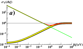
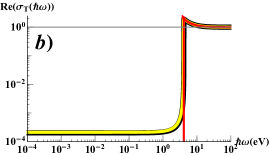
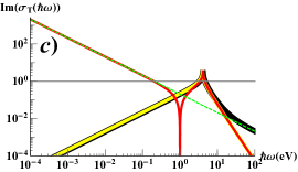
Figure 1: (Color online) Double logarithmic plots of the real part of the transversal conductivity $\sigma_{T}$ (in units of the universal conductivity of graphene $\sigma_{0}=\frac{\alpha c}{4}$) as a function of the imaginary frequency $\hbar\omega=\mathrm{i}\hbar\xi$ in panel (a), the real part for real frequency $\hbar\omega$ in panel (b) and the imaginary part for real frequencies in (c), for the case with $k_{B}T=\mu=0$, $\Delta=2\text{ eV}$, $\tilde{q}_{\parallel}=1\text{ eV}$ and dissipation rate $\hbar\Gamma=10^{-3}\text{ eV}$. The thick black curve is the non-local conductivity derived from the Kubo formula, given in this limit by Eq. (171), the red curve is the non-local conductivity $\sigma_{T,0}^{QFT-b}(\omega,\tilde{q}_{\parallel})$ show in Eq. (169), the yellow curve is the local conductivity show in Eq. (136) and the green curve is the $\hbar\xi\to 0$ divergence of Eq. (169), given in Eq. (170). The dashed curves in panel (c) represent the positive imaginary parts of the conductivity, while the full curves represent the negative values.

VIII Numerical comparison

In the following figures, we compare the longitudinal and transversal conductivities derived from the 3 models we have studied here. We compared for different temperatures $T$, chemical potentials $\mu$, mass gaps $\Delta$ and momentum $\tilde{q}$, the longitudinal (Fig. 2) and transversal conductivities (Fig. 3) derived from the three different models studied here. The local limit ($\tilde{q}_{\parallel}=0$) at $T=0\text{ K}$ and $T=300\text{ K}$ are represented by the thick black and the yellow dashed curves respectively. The non-local conductivities derived from the Kubo formula with $\tilde{q}_{\parallel}\neq 0\text{ eV}$ and $\hbar\Gamma=10^{-3}\text{ eV}$ at $T=0\text{ K}$ and $T=300\text{ K}$ are represented by the thick red and the blue dashed curves respectively. The non-local conductivity derived from the QFT-b model with $\tilde{q}_{\parallel}\neq 0\text{ eV}$ at $T=0\text{ K}$ and $T=300\text{ K}$ are represented by the dashed brown and thick green curve respectively. We study the non-locality for $\tilde{q}_{\parallel}=10^{-2}\text{ eV}$ and for $\tilde{q}_{\parallel}=1\text{ eV}$.

As can be observed in Fig. 2, the results for the non-local longitudinal conductivities derived from the Kubo formula and from the QFT-b model almost coincide. Actually, if we artificially add the (non-existant) dissipation rate $\hbar\Gamma$ to the QFT-b model, the two curves would almost superimpose, with any difference explained by the use of different regularizations of the integrals. This fact remarks the contribution the electronic quasi-particle dissipation has in the conductivity, mainly for frequencies $\left|\omega\right|\lesssim\Gamma$.

As can be observed in Figs. 3, the results for the non-local transversal conductivities derived from the Kubo formula and from the QFT-b model are very different. The main problem here is that an spurious asymptote proportional to $(\hbar\xi)^{-1}$ appears for very small imaginary frequencies. This difference is explained because $\sigma_{T}^{QFT-b}(\mathrm{q})$ does not fulfil the Gauge invariance imposed condition $\displaystyle\lim_{\omega\to 0}\Pi^{\mu\nu}(\omega)A_{\nu}(\omega)=0$ for constant static $A_{\nu}(\omega)$.

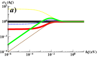
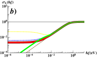
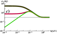
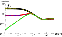
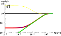
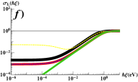
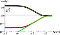
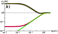
Figure 2: (Color online) Double logarithmic plots of the longitudinal conductivity $\sigma_{L}(\mathrm{i}\hbar\xi)$ (in units of the universal conductivity of graphene $\sigma_{0}=\frac{\alpha c}{4}$) as a function of the imaginary frequency $\hbar\omega=\mathrm{i}\hbar\xi$. The thick black and the yellow dashed curves are the local conductivity ($\tilde{q}_{\parallel}=0$) at $T=0\text{ K}$ and $T=300\text{ K}$ respectively. The thick red and the blue dashed curves are the non-local conductivities derived from the Kubo formula with $\tilde{q}_{\parallel}\neq 0$, $\hbar\Gamma=10^{-3}\text{ eV}$ at $T=0\text{ K}$ and $T=300\text{ K}$ respectively. The tick green and brown dashed curves are the non-local conductivity derived from the QFT-b model with $\tilde{q}\neq 0$ at $T=300\text{ K}$ and $T=0\text{ K}$ respectively, finally, the thin gray line is the universal conductivity of graphene with $\sigma(\mathrm{i}\hbar\xi)=\sigma_{0}=\frac{\alpha c}{4}$. In a) $\{\mu,\Delta,\tilde{q}_{\parallel}\}=\{0,0,10^{-2}\}\text{ eV}$, in b) $\{\mu,\Delta,\tilde{q}_{\parallel}\}=\{0,0.2,10^{-2}\}\text{ eV}$, in c) $\{\mu,\Delta,\tilde{q}_{\parallel}\}=\{0.25,0,10^{-2}\}\text{ eV}$, in d) $\{\mu,\Delta,\tilde{q}_{\parallel}\}=\{0.25,0.2,10^{-2}\}\text{ eV}$, in e) $\{\mu,\Delta,\tilde{q}_{\parallel}\}=\{0,0,1\}\text{ eV}$, in f) $\{\mu,\Delta,\tilde{q}_{\parallel}\}=\{0,0.2,1\}\text{ eV}$, in g) $\{\mu,\Delta,\tilde{q}_{\parallel}\}=\{0.25,0,1\}\text{ eV}$, and in h) $\{\mu,\Delta,\tilde{q}_{\parallel}\}=\{0.25,0.2,1\}\text{ eV}$.

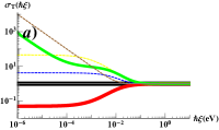
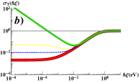
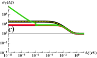
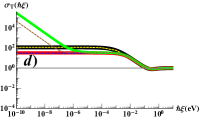
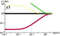
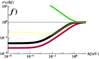
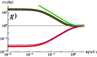
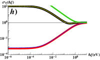
Figure 3: (Color online) Double logarithmic plots of the transversal conductivity $\sigma_{T}(\mathrm{i}\hbar\xi)$ (in units of the universal conductivity of graphene $\sigma_{0}=\frac{\alpha c}{4}$) as a function of the imaginary frequency $\hbar\omega=\mathrm{i}\hbar\xi$. The thick black and the yellow dashed curves are the local conductivity ($\tilde{q}_{\parallel}=0$) at $T=0\text{ K}$ and $T=300\text{ K}$ respectively. The thick red and the blue dashed curves are the non-local conductivities derived from the Kubo formula with $\tilde{q}_{\parallel}\neq 0$, $\hbar\Gamma=10^{-3}\text{ eV}$ at $T=0\text{ K}$ and $T=300\text{ K}$ respectively. The tick green and brown dashed curves are the non-local conductivity derived from the QFT-b model with $\tilde{q}_{\parallel}\neq 0$ at $T=300\text{ K}$ and $T=0\text{ K}$ respectively, finally, the thin gray line is the universal conductivity of graphene with $\sigma(\mathrm{i}\hbar\xi)=\sigma_{0}=\frac{\alpha c}{4}$. In a) $\{\mu,\Delta,\tilde{q}_{\parallel}\}=\{0,0,10^{-2}\}\text{ eV}$, in b) $\{\mu,\Delta,\tilde{q}_{\parallel}\}=\{0,0.2,10^{-2}\}\text{ eV}$, in c) $\{\mu,\Delta,\tilde{q}_{\parallel}\}=\{0.25,0,10^{-2}\}\text{ eV}$, in d) $\{\mu,\Delta,\tilde{q}_{\parallel}\}=\{0.25,0.2,10^{-2}\}\text{ eV}$, in e) $\{\mu,\Delta,\tilde{q}_{\parallel}\}=\{0,0,1\}\text{ eV}$, in f) $\{\mu,\Delta,\tilde{q}_{\parallel}\}=\{0,0.2,1\}\text{ eV}$, in g) $\{\mu,\Delta,\tilde{q}_{\parallel}\}=\{0.25,0,1\}\text{ eV}$, and in h) $\{\mu,\Delta,\tilde{q}_{\parallel}\}=\{0.25,0.2,1\}\text{ eV}$.

IX Conclusions

In this article we have shown a detailed derivation of the polarization $\Pi$ and conductivity $\sigma$ of graphene close to the Dirac point in the continuous limit. We have used the Kubo formula [4] ($\sigma^{K}$), a Quantum Field Theory based (QFT-b) model (which approaches the electronic quasiparticles as $(2+1)D$ Dirac electrons) [6] ($\sigma^{QFT-b}$) and a local model [17] ($\sigma^{F}$).

The more general result is obtained with the Kubo formula $\sigma^{K}$. This result is valid for any complex frequency (with positive imaginary part) $\omega\in\mathbb{C}^{+}$, constant dissipation rate $\Gamma$, chemical potential $\mu$ and Dirac mass $m$ as a closed analytical formula at zero Temperature $T$. The non-zero temperature results can be obtained after an integration by using the Maldague formula (Eq. (135)).

We obtain that the local limit of $\sigma^{K}$ is actually $\sigma^{F}$ if we make $m=0$ and the dissipation of the interband conductivity exactly zero.

We have derived the polarization (and, therefore, the conductivity) as in the QFT-b model, we obtain again the results published elsewhere, and we find that the longitudinal conductivity derived from the Kubo formula and from the QFT-b model almost coincide, with any difference explained by the different regularization strategies used. However, there is not such a coincidence with the transversal conductivity. The main difference come from the regularization of the polarization operator used. In the case of the Kubo formula, the expression of the polarization operator is regularized by imposing that, because of the Gauge invariance of the theory, $\displaystyle\lim_{\omega\to 0}\Pi^{\mu\nu}(\omega)A_{\nu}(\omega)=0$ for constant static $A_{\nu}(\omega)$ [42]. This regularization also makes the Kubo formula integrable for Dirac electrons without the need of an upper cut-off (in $(2+1)D$, in $(3+1)D$ the cut-off is still needed [69]). By the contrary, in the derivation of the QFT-b model, the Gauge invariance is not imposed and the divergent integrals are regularized by other means (like the Pauli-Villars subtraction scheme [18]). As a consequence, the Longitudinal conductivity derived from the QFT-b model coincides with the result derived from the Kubo formula because it accidentally fulfils the Gauge invariance of the theory, but the Transversal conductivity does not coincide because the QFT-b result has $\displaystyle\lim_{\omega\to 0}\Pi_{T}(\omega)\neq 0$.

If a system does not fulfil the Gauge invariance condition, we would have a physical effect (a static electronic conductivity $\bm{j}(0)$) dependent of a Gauge invariant quantity (the constant static potential vector $A_{\nu}(0)$ [12] [42]), something forbidden in Gauge invariant theories.

We show how to correctly regularize the QFT-b model in order to satisfy the gauge invariance, once the correct regularization done, the Kubo and QFT-b model exactly coincide for all parameters of the model.

This result can affect to the prediction of the Casimir effect with graphene.

Appendix A Non-local Kubo conductivity expressions

The analytical formulas for the non-local conductivities of 2D Dirac cones have been derived in [4] from Eq. (103). Those formulas are naturally splitted into 2 parts, one independent of the chemical potential $\mu$ and another term for which the chemical potential is accounted for. Namely, $\sigma_{p}(\mathrm{q})=\sigma_{p,0}(\mathrm{q})+\Theta(|\mu|-|\Delta|)\sigma_{p,1}(\mathrm{q})$, where $\Theta$ is the Heaviside step function and $p=\{L,T,H\}$. Using the parameters $\tilde{\theta}_{z}=\sqrt{\tilde{q}_{\parallel}^{2}-\tilde{q}_{0}^{2}}$, $\gamma=\frac{\Xi}{\tilde{\theta}_{z}}$, $\delta=\frac{2|\Delta|}{\tilde{\theta}_{z}}$, and

$$\Psi(x)=2\left[x+\left(1-x^{2}\right)\tan^{-1}\left(\dfrac{1}{x}\right)\right],$$ (172)

$$\sigma_{L,0}(\mathrm{q}) = \frac{\sigma_{0}}{2\pi}\frac{-\mathrm{i}\tilde{q}_{0}}{\tilde{\theta}_{z}^{2}}\left[2|\Delta|+\frac{\tilde{\theta}_{z}^{2}-4\Delta^{2}}{\tilde{\theta}_{z}}\tan^{-1}\left(\dfrac{\tilde{\theta}_{z}}{2|\Delta|}\right)\right]=\frac{\sigma_{0}}{4\pi}\frac{-\mathrm{i}\tilde{q}_{0}}{\tilde{\theta}_{z}}\Psi(\delta),$$ (173)

$$\sigma_{L,1}(\mathrm{q}) = \frac{\sigma_{0}}{2\pi}\frac{-\mathrm{i}\tilde{q}_{0}}{\tilde{q}_{\parallel}^{2}}\left[4(|\mu|-|\Delta|)+\frac{1}{2\tilde{\theta}_{z}}\left(\mathcal{F}_{1}+\left(R^{2}-\tilde{q}_{\parallel}^{2}\right)\mathcal{F}_{2}\right)+\frac{\tilde{q}_{\parallel}}{q_{0}^{2}}\Theta\left(\tilde{q}_{\parallel}^{2}-4\left(\mu^{2}-\Delta^{2}\right)\right)\mathcal{F}_{3}\right],$$ (174)

$$\sigma_{T,0}(\mathrm{q}) = \frac{\sigma_{0}}{2\pi}\frac{1}{-\mathrm{i}\tilde{q}_{0}}\left[\frac{\tilde{\theta}_{z}^{2}-4\Delta^{2}}{\tilde{\theta}_{z}}\tan^{-1}\left(\frac{\tilde{\theta}_{z}}{2|\Delta|}\right)-\frac{\tilde{q}_{\parallel}^{2}-4\Delta^{2}}{\tilde{q}_{\parallel}}\tan^{-1}\left(\frac{\tilde{q}_{\parallel}}{2|\Delta|}\right)\right]=\frac{\sigma_{0}}{4\pi}\frac{1}{-\mathrm{i}\tilde{q}_{0}}\left[\tilde{\theta}_{z}\Psi(\delta)-\tilde{q}_{\parallel}\Psi(x)\right],$$ (175)

$$\sigma_{T,1}(\mathrm{q}) = \frac{\sigma_{0}}{2\pi}\frac{\mathrm{i}}{q_{0}}\!\!\left[4\frac{\tilde{q}_{0}^{2}}{\tilde{q}_{\parallel}^{2}}4(|\mu|-|\Delta|)+2|\Delta|-\frac{1}{2\tilde{\theta}_{z}}\left(\frac{\tilde{\theta}_{z}^{2}}{\tilde{q}_{\parallel}^{2}}\mathcal{F}_{1}+\left(\tilde{\theta}_{z}^{2}-4\Delta^{2}\right)\mathcal{F}_{2}\right)\right.$$ (176)

$$\left.\leavevmode\nobreak\ \leavevmode\nobreak\ \leavevmode\nobreak\ \leavevmode\nobreak\ \leavevmode\nobreak\ \leavevmode\nobreak\ \leavevmode\nobreak\ \leavevmode\nobreak\ +\frac{1}{\tilde{q}_{\parallel}}\left(\mathcal{F}_{4}\Theta\left(\tilde{q}_{\parallel}^{2}-4\left(\mu^{2}-\Delta^{2}\right)\right)+\mathcal{F}_{5}\Theta\left(4\left(\mu^{2}-\Delta^{2}\right)-\tilde{q}_{\parallel}^{2}\right)\right)\right],$$

$$\sigma_{H,0}(\mathrm{q}) = \frac{2\sigma_{0}}{\pi}\frac{\eta\Delta}{\tilde{\theta}_{z}}\tan^{-1}\left(\frac{\tilde{\theta}_{z}}{2|\Delta|}\right),$$ (177)

$$\sigma_{H,1}(\mathrm{q}) = -\frac{\sigma_{0}}{\pi}\frac{\eta\Delta}{\tilde{\theta}_{z}}\left[\tan^{-1}\left(\frac{\tilde{q}_{0}-2|\Delta|}{\sqrt{R^{2}-(\tilde{q}_{0}-2|\Delta|)^{2}}}\right)-\tan^{-1}\left(\frac{\tilde{q}_{0}-2|\mu|}{\sqrt{R^{2}-(\tilde{q}_{0}-2|\mu|)^{2}}}\right)\right.$$ (179)

$$\left.\leavevmode\nobreak\ \leavevmode\nobreak\ \leavevmode\nobreak\ \leavevmode\nobreak\ \leavevmode\nobreak\ \leavevmode\nobreak\ \leavevmode\nobreak\ \leavevmode\nobreak\ \leavevmode\nobreak\ \leavevmode\nobreak\ \leavevmode\nobreak\ \leavevmode\nobreak\ \leavevmode\nobreak\ +\mathrm{i}\log\left(\frac{\tilde{q}_{0}+2|\mu|+\sqrt{(\tilde{q}_{0}+2|\mu|)^{2}-R^{2}}}{\tilde{q}_{0}+2|\Delta|+\sqrt{(\tilde{q}_{0}+2|\Delta|)^{2}-R^{2}}}\right)\right],$$

where $\sigma_{0}=\frac{\alpha c}{4}=\frac{e^{2}}{4\hbar}$, $\tilde{q}_{0}=\hbar\Omega=\hbar\omega+\mathrm{i}\hbar\Gamma$ ($\Gamma=\tau^{-1}$ accounts for the relaxation time), $\tilde{q}_{\parallel}=\hbar v_{F}q$, $\tilde{\theta}_{z}=\sqrt{\tilde{q}_{\parallel}^{2}-\tilde{q}_{0}^{2}}$, $R=\tilde{q}_{\parallel}\sqrt{1+4(|\Delta|/\tilde{\theta}_{z})^{2}}$, $\delta=\frac{2\Delta}{\tilde{\theta}_{z}}$ and $x=\frac{2\Delta}{\tilde{q}_{\parallel}}$. It is important to note that only the modulus of the mass gaps enter into the expressions for $\sigma_{L}$ and $\sigma_{T}$, while $\sigma_{H}$ has an additional dependency on the sign of the gaps through the combination $\eta\Delta^{\eta}_{s}$. The auxiliary functions $\{\mathcal{F}_{n}\}_{n=1}^{5}$ depend on $q_{0}$, $\mu$, $|\Delta|$, $\tilde{q}_{\parallel}$, and $R$, and are the following

$$\mathcal{F}_{1} = \phantom{+\mathrm{i}}(\tilde{q}_{0}-2|\mu|)\sqrt{R^{2}-(\tilde{q}_{0}-2|\mu|)^{2}}-\phantom{\mathrm{i}}(\tilde{q}_{0}-2|\Delta|)\sqrt{R^{2}-(\tilde{q}_{0}-2|\Delta|)^{2}}$$ (180)

$$+\mathrm{i}(\tilde{q}_{0}+2|\mu|)\sqrt{(\tilde{q}_{0}+2|\mu|)^{2}-R^{2}}-\mathrm{i}(\tilde{q}_{0}+2|\Delta|)\sqrt{(\tilde{q}_{0}+2|\Delta|)^{2}-R^{2}},$$

$$\mathcal{F}_{2} = \phantom{-\mathrm{i}}\tan^{-1}\left(\frac{\tilde{q}_{0}-2|\Delta|}{\sqrt{R^{2}-(\tilde{q}_{0}-2|\Delta|)^{2}}}\right)-\tan^{-1}\left(\frac{\tilde{q}_{0}-2|\mu|}{\sqrt{R^{2}-(\tilde{q}_{0}-2|\mu|)^{2}}}\right)$$ (181)

$$-\mathrm{i}\log\left(\tilde{q}_{0}+2|\Delta|+\sqrt{(\tilde{q}_{0}+2|\Delta|)^{2}-R^{2}}\right)+\mathrm{i}\log\left(\tilde{q}_{0}+2|\mu|+\sqrt{(\tilde{q}_{0}+2|\mu|)^{2}-R^{2}}\right),$$

$$\mathcal{F}_{3} = \phantom{+}2\mu\left(\sqrt{\tilde{q}_{\parallel}^{2}-4\left(\mu^{2}-\Delta^{2}\right)}+\mathrm{i}\sqrt{4\left(\mu^{2}-\Delta^{2}\right)-\tilde{q}_{\parallel}^{2}}\right)$$ (185)

$$+\left(4\Delta^{2}-\tilde{q}_{\parallel}^{2}\right)\left[\begin{array}[]{l}\mathrm{i}\log(2|\Delta|+\mathrm{i}\tilde{q}_{\parallel})-\mathrm{i}\log\left(2|\mu|+\sqrt{4\left(\mu^{2}-\Delta^{2}\right)-\tilde{q}_{\parallel}^{2}}\right)\\ \end{array}\right]$$

$$+\left(4\Delta^{2}-\tilde{q}_{\parallel}^{2}\right)\left[\begin{array}[]{l}\tan^{-1}\left(\frac{2|\mu|}{\sqrt{\tilde{q}_{\parallel}^{2}-4(\mu^{2}-\Delta^{2})}}\right)-\tan^{-1}\left(\frac{2|\Delta|}{\tilde{q}_{\parallel}}\right)\end{array}\right],$$

$$\mathcal{F}_{4} = -2|\mu|\sqrt{\tilde{q}_{\parallel}^{2}-4\left(\mu^{2}-\Delta^{2}\right)}+\left(\tilde{q}_{\parallel}^{2}-4\Delta^{2}\right)\left[\tan^{-1}\left(\frac{2|\mu|}{\sqrt{\tilde{q}_{\parallel}^{2}-4(\mu^{2}-\Delta^{2})}}\right)-\tan^{-1}\left(\frac{2|\Delta|}{\tilde{q}_{\parallel}}\right)\right],$$ (186)

$$\mathcal{F}_{5} = \left(\tilde{q}_{\parallel}^{2}-4\Delta^{2}\right)\left[\frac{\pi}{2}-\tan^{-1}\left(\frac{2|\Delta|}{\tilde{q}_{\parallel}}\right)\right].$$ (187)

Those results are valid for all frequencies $\omega\in\mathbb{C}^{+}$, and we remind that they are the conductivity per Dirac cone, to obtain the conductivity of Graphene, we must to sum the contribution of each 4 Dirac cones, having into account their respective (signed) Dirac masses by using

$$\sigma_{p}(\mathrm{q})=\sum_{\eta=\pm}\sum_{s=\pm}\sigma_{p}(\mathrm{q},\Delta_{s}^{\eta})$$ (188)

Appendix B Local Kubo conductivity expressions

There is an special case in the local limit (when we apply the $\bm{q}_{\parallel}\to\bm{0}$ limit to the Kubo formula (103)) when results valid for all temperatures can be obtained. The local limit of the conductivities of a massive Dirac cone are

$$\sigma_{xx}(\omega,\bm{0},\mu,\Delta) = \mathrm{i}\frac{\sigma_{0}}{\pi}\Bigg{[}\frac{\mu^{2}-\Delta^{2}}{|\mu|}\frac{1}{\Omega}\Theta\left(|\mu|-|\Delta|\right)+\frac{\Delta^{2}}{M\Omega}-\frac{\Omega^{2}+4\Delta^{2}}{2i\Omega^{2}}\tan^{-1}\left(\frac{i\Omega}{2M}\right)\Bigg{]},$$ (189)

$$\sigma_{xy}(\omega,\bm{0},\mu,\Delta) = \frac{2\sigma_{0}}{\pi}\frac{\eta\Delta}{i\Omega}\tan^{-1}\left(\frac{i\Omega}{2M}\right),$$ (190)

where $\Omega=\hbar\omega+\mathrm{i}\hbar\Gamma$, $\Gamma=\tau^{-1}$ and $M=\text{Max}\left[|\Delta|,|\mu|\right]$. These results are per Dirac cone and they are consistent with the ones found by other researchers [16][17][18][19][60][61][62][63]. The first term in $\sigma_{xx}$ corresponds to intra-band transitions, and the last two terms to inter-band transitions. Note that, in the local limit $\bm{q}_{\parallel}\to\bm{0}$ one obtains $\sigma_{xx}(\omega,0)=\sigma_{yy}(\omega,0)=\sigma_{L}(\omega,0)=\sigma_{T}(\omega,0)$, and $\sigma_{xy}(\omega,0)=-\sigma_{yx}(\omega,0)=\sigma_{H}(\omega,0)$.

From those results, we obtain the conductivity at zero temperature of a Dirac cone with $\Delta=0$ mass gap as

$$\sigma_{xx}(\omega,\bm{q}_{\parallel}=\bm{0},T=0,\Delta=0) = \sigma^{\text{intra}}_{xx}(\omega)+\sigma^{\text{inter}}_{xx}(\omega)$$

$$\sigma^{\text{intra}}_{xx}(\omega) = \dfrac{\alpha c}{\pi}\dfrac{|\mu|}{-\mathrm{i}\Omega}$$

$$\sigma^{\text{inter}}_{xx}(\omega) = \dfrac{\alpha c}{2\pi}\tan^{-1}\left(\dfrac{-\mathrm{i}\Omega}{2|\mu|}\right)$$

$$\sigma_{xy}(\omega,\bm{q}_{\parallel}=\bm{0},T=0,\Delta=0) = 0,$$ (191)

From this result with $\Delta=0$, in the non-dissipation limit for the interband term and for finite temperatures, by using the Maldague formula, the well-known result of Falkovsky is obtained as

$$\sigma^{F}_{xx}(\omega,\Gamma,T,\mu) = \sigma^{F,\text{intra}}_{xx}(\omega,\Gamma,T,\mu)+\sigma^{F,\text{inter}}_{xx}(\omega,0,T,\mu)$$

$$\sigma^{F,\text{intra}}_{xx}(\omega,\Gamma,T,\mu) = \dfrac{1}{\pi\hbar}\dfrac{2\mathrm{i}\alpha ck_{\rm B}T}{\omega+\mathrm{i}\Gamma}\ln\left[2\cosh\left(\frac{\mu}{2k_{\rm B}T}\right)\right]$$

$$\sigma^{F,\text{inter}}_{xx}(\omega,\Gamma,T,\mu) = \dfrac{\alpha c}{4}G\left(\left|\dfrac{\hbar\omega}{2}\right|\right)+\mathrm{i}\dfrac{\alpha c}{4}\dfrac{4\hbar\omega}{\pi}\int_{0}^{\infty}\mathrm{d}\xi\frac{G(\xi)-G\left(\dfrac{\hbar\omega}{2}\right)}{(\hbar\omega)^{2}-4\xi^{2}}$$ (192)

with

$$G\left(\dfrac{\hbar\omega}{2}\right)=n_{F}(-\epsilon+\mu)-n_{F}(+\epsilon+\mu)=\dfrac{\sinh\left(\beta\epsilon\right)}{\cosh\left(\beta\mu\right)+\cosh\left(\beta\epsilon\right)}.$$ (193)

The intraband term is obtained by the use of the Maldague formula (Eq. (135)) for Eq. (VI), as

$$\sigma^{\text{intra}}_{xx}(\omega,T) = \dfrac{\alpha c}{\pi}\dfrac{1}{-\mathrm{i}\Omega}\frac{2}{\beta}\ln\left[2\cosh\left(\frac{\beta\mu}{2}\right)\right]=\dfrac{\alpha c}{\pi\hbar}\dfrac{2\mathrm{i}k_{\rm B}T}{\omega+\mathrm{i}\Gamma}\ln\left[2\cosh\left(\frac{\mu}{2k_{\rm B}T}\right)\right].$$ (194)

To derive the local interband conductivity at finite temperatures, we first need to apply the zeroth dissipation limit $\tau\to\infty$ ($\Gamma\to 0$) of the real part $\omega\in\mathbb{R}$ of the interband conductivity of graphene, as

$$\lim_{\tau\to\infty}\mathbb{R}\text{e}\left[\sigma^{\text{inter}}_{xx}(\omega)\right]=\lim_{\tau\to\infty}\dfrac{\alpha c}{2\pi}\tan^{-1}\left(\dfrac{-\mathrm{i}\Omega}{2|\mu|}\right)=\dfrac{\alpha c}{4}\Big{[}\Theta\left(\hbar\omega-2|\mu|\right)+\Theta\left(-\hbar\omega-2|\mu|\right)\Big{]},$$ (195)

which coincides with the result shown in [17] in the $T\to 0$ limit for $\omega>0$. Note that $\mathbb{R}\text{e}\left[\sigma^{\text{inter}}_{xx}(-\omega)\right]=+\mathbb{R}\text{e}\left[\sigma^{\text{inter}}_{xx}(\omega)\right]$ is an even function in $\omega$.

Applying the Maldague formula (Eq. (135)) to Eq.(VI), we obtain

$$\mathbb{R}\text{e}\left[\sigma^{\text{inter}}_{xx}(\omega,\mu,T)\right]=G\left(\left|\dfrac{\hbar\omega}{2}\right|\right)=\dfrac{\alpha c}{4}\left(\dfrac{1}{e^{\beta\left(\mu-|\frac{\hbar\omega}{2}|\right)}+1}-\dfrac{1}{e^{\beta\left(\mu+|\frac{\hbar\omega}{2}|\right)}+1}\right)=\dfrac{\alpha c}{4}\dfrac{\sinh\left(\beta|\frac{\hbar\omega}{2}|\right)}{\cosh\left(\beta\mu\right)+\cosh\left(\beta|\frac{\hbar\omega}{2}|\right)}.$$ (196)

We have the absolute value in the formula above because we are handling also negative real frequencies, while in [17] the result for only positive frequencies where derived. Applying a regularized version of the Kramers-Krönig relationships that avoids the use of the principal part of a function, that read as [70][71][72]:

$$\sigma_{R}(x)=\frac{2}{\pi}\int_{0}^{\infty}\mathrm{d}\omega\frac{\omega\sigma_{I}(\omega)-x\sigma_{I}(x)}{\omega^{2}-x^{2}}$$

$$\sigma_{I}(x)=\frac{2}{\pi}x\int_{0}^{\infty}\mathrm{d}\omega\frac{\sigma_{R}(x)-\sigma_{R}(\omega)}{\omega^{2}-x^{2}}$$ (197)

it is immediate that

$$\mathbb{I}\text{m}\left[\sigma^{\text{inter}}(\omega,T)\right]=\dfrac{4\hbar\omega}{\pi}\int_{0}^{\infty}\mathrm{d}\xi\frac{G(\xi)-G\left(\left|\dfrac{\hbar\omega}{2}\right|\right)}{(\hbar\omega)^{2}-4\xi^{2}},$$ (198)

which coincides with the imaginary part of the interband term of Fialkovsky [73].

Finally, by using the Kramers-Krönig relation to find the real part of the conductivity at imaginary frequencies $\omega=\mathrm{i}\xi$ [44]

$$\mathbb{R}\text{e}\left[\sigma_{p,0}(\mathrm{i}\xi)\right] = \frac{2}{\pi}\int_{0}^{\infty}d\omega\frac{\xi}{\omega^{2}+\xi^{2}}\mathbb{R}\text{e}\left[\sigma_{p,0}(\omega)\right]=\frac{2}{\pi}\int_{0}^{\infty}d\omega\frac{\omega}{\omega^{2}+\xi^{2}}\mathbb{I}\text{m}\left[\sigma_{p,0}(\omega)\right],$$ (199)

we obtain the interband conductivity for imaginary frequencies as [9]

$$\sigma_{F}^{\text{inter}}(\mathrm{i}\hbar\xi) = \frac{2}{\pi}\int_{0}^{\infty}d\omega\frac{\hbar\xi}{(\hbar\omega)^{2}+(\hbar\xi)^{2}}G\left(\frac{\hbar\omega}{2}\right).$$ (200)

Note that this result is completely equivalent to the use of the Maldague formula to $\sigma_{xx}^{\text{inter}}$ given in Eq. (B), and by making the substitution $\xi\rightarrow\xi+\Gamma$, we can automatically add the constant dissipation to this interband conductivity.

Appendix C Quantum Field Theory based model for the conductivity

In this appendix we will show how to derive the results for the polarization operator given in [5][13][6] presented in section VII from Eq. (143).

$$\Pi^{\mu\nu}(\mathrm{q})=\mathrm{i}g_{s}\dfrac{\alpha c}{\hbar}\int_{k}\dfrac{Z^{\mu\nu}(K_{\alpha},q_{\alpha})}{\left[K^{\mu}K_{\mu}-m^{2}\right]\left[S^{\mu}S_{\mu}-m^{2}\right]},$$ (201)

We are going to use the following notation: $S_{\mu}=K_{\mu}+q_{\mu}$, $K_{\mu}=(\tilde{k}_{0}+\mu,\tilde{\bm{k}}_{\parallel})=(\mathrm{i}\hbar\omega_{n}+\mu,\hbar v_{F}\bm{k}_{\parallel})$, $q_{\mu}=(\tilde{q}_{0},\tilde{\bm{q}}_{\parallel})=(\hbar\omega,\hbar v_{F}\bm{q}_{\parallel})$ (see tab. 1), $Z^{\mu\nu}(K_{\alpha},q_{\alpha})$ is given in Eq. (148).

We apply the Matsubara formalism directly to the expression of Eq. (201) to obtain the expression shown in [6]. Remembering that, for fermions we have $\tilde{k}_{0}=\hbar\omega_{n}=\frac{2\pi}{\beta}\left(n+\frac{1}{2}\right)$ $\forall n\in\mathbb{Z}$, we obtain

$$\dfrac{\hbar\Pi^{\mu\nu}(\mathrm{q})}{\mathrm{i}g_{s}\alpha c} = \int_{-\infty}^{\infty}\dfrac{\mathrm{d}\tilde{k}_{0}}{2\pi}\dfrac{Z^{\mu\nu}(\tilde{k}_{0}+\mu,\tilde{\bm{k}}_{\parallel},\tilde{q}_{0},\tilde{\bm{q}}_{\parallel})}{\left[K^{\mu}K_{\mu}-m^{2}\right]\left[S^{\mu}S_{\mu}-m^{2}\right]}$$ (202)

$$= \int_{-\infty}^{\infty}\dfrac{\mathrm{d}\tilde{k}_{0}}{2\pi}\dfrac{Z^{\mu\nu}(\tilde{k}_{0}+\mu,\tilde{\bm{k}}_{\parallel},\tilde{q}_{0},\tilde{\bm{q}}_{\parallel})}{\left[(\tilde{k}_{0}+\mu)^{2}-\epsilon_{\bm{k}}^{2}\right]\left[(\tilde{k}_{0}+\tilde{q}_{0}+\mu)^{2}-\epsilon_{\bm{k}+\bm{q}}^{2}\right]}$$

$$= \frac{1}{\beta}\sum_{n\in\mathbb{Z}}^{\text{Fermi}}\dfrac{Z^{\mu\nu}(\mathrm{i}\hbar\omega_{n}+\mu,\tilde{\bm{k}}_{\parallel},\tilde{q}_{0},\tilde{\bm{q}}_{\parallel})}{\left[(\mathrm{i}\hbar\omega_{n}+\mu)^{2}-\epsilon_{\bm{k}}^{2}\right]\left[(\mathrm{i}\hbar\omega_{n}+\tilde{q}_{0}+\mu)^{2}-\epsilon_{\bm{s}}^{2}\right]}$$

$$= \left[\dfrac{Z_{\mu\nu}(-\tilde{q}_{0}-\epsilon_{\bm{s}},\tilde{\bm{k}}_{\parallel},\tilde{q}_{0},\tilde{\bm{q}}_{\parallel})}{2\epsilon_{\bm{s}}\left((\tilde{q}_{0}+\epsilon_{\bm{s}})^{2}-\epsilon_{\bm{k}}^{2}\right)}+\dfrac{Z_{\mu\nu}(-\epsilon_{\bm{k}},\tilde{\bm{k}}_{\parallel},\tilde{q}_{0},\tilde{\bm{q}}_{\parallel})}{2\epsilon_{\bm{k}}((\tilde{q}_{0}-\epsilon_{\bm{k}})^{2}-\epsilon_{\bm{s}}^{2})}\right]$$

$$-\sum_{\lambda=\pm}\dfrac{n_{F}(\epsilon_{\bm{s}}-\lambda\mu)Z_{\mu\nu}(-\tilde{q}_{0}+\epsilon_{\bm{s}}^{\lambda},\tilde{\bm{k}}_{\parallel},\tilde{q}_{0},\tilde{\bm{q}}_{\parallel})}{2\epsilon_{\bm{s}}\left((\tilde{q}_{0}-\epsilon_{\bm{s}}^{\lambda})^{2}-\epsilon_{\bm{k}}^{2}\right)}-\sum_{\lambda=\pm}\dfrac{n_{F}(\epsilon_{\bm{k}}-\lambda\mu)Z_{\mu\nu}(\epsilon_{\bm{k}}^{\lambda},\tilde{\bm{k}}_{\parallel},\tilde{q}_{0},\tilde{\bm{q}}_{\parallel})}{2\epsilon_{\bm{k}}\left((\tilde{q}_{0}+\epsilon_{\bm{k}}^{\lambda})^{2}-\epsilon_{\bm{s}}^{2}\right)}$$

with $\bm{s}_{\parallel}=\bm{k}_{\parallel}+\bm{q}_{\parallel}$ (see tab. 1). The term in brackets corresponds to the integrand of the $T=0$ limit, while the second and third terms correspond to the correction due to the temperature. Therefore, following the notation of [6], the Polarization operator given in Eq. (201) can be written as

$$\Pi^{\mu\nu}(\mathrm{q})=\Pi_{0}^{\mu\nu}(\mathrm{q})+\Delta_{T}\Pi^{\mu\nu}(\mathrm{q}),$$ (203)

by construction, $\Pi_{0}^{\mu\nu}(\mathrm{q})$ is independent of temperature and of the chemical potential $\mu$ [6], therefore, it corresponds to the interband conductivity with $\mu=k_{B}T=0\text{ eV}$. On the other hand, to simplify $\Delta_{T}\Pi^{\mu\nu}(\mathrm{q})$, we apply the change of variables $\bm{k}_{\parallel}\to-(\bm{k}_{\parallel}+\bm{q}_{\parallel})$, we also make use of the symmetry of the relation of dispersion $\epsilon_{\bm{k}}=\epsilon_{-\bm{k}}$ and we transform the dummy variable $\lambda\to-\lambda$ to the first summand of $\Delta_{T}\Pi^{\mu\nu}(q)$ to obtain

$$\displaystyle\int_{BZ}\dfrac{\mathrm{d}^{2}\bm{k}_{\parallel}}{(2\pi)^{2}}\sum_{\lambda=\pm}\dfrac{n_{F}(\epsilon_{\bm{s}}-\lambda\mu)Z_{\mu\nu}(-\tilde{q}_{0}+\epsilon_{\bm{s}}^{\lambda},\tilde{\bm{k}}_{\parallel},\tilde{q}_{0},\tilde{\bm{q}}_{\parallel})}{2\epsilon_{\bm{s}}\left((\tilde{q}_{0}-\epsilon_{\bm{s}}^{\lambda})^{2}-\epsilon_{\bm{k}}^{2}\right)} = \displaystyle\int_{\bm{k}}\sum_{\lambda=\pm}\dfrac{n_{F}(\epsilon_{-\bm{k}}+\lambda\mu)Z_{\mu\nu}(-\tilde{q}_{0}-\epsilon_{-\bm{k}}^{\lambda},-\tilde{\bm{s}}_{\parallel},\tilde{q}\tilde{q}_{0},\tilde{\bm{q}}_{\parallel})}{2\epsilon_{-\bm{k}}\left((\tilde{q}_{0}+\epsilon_{-\bm{k}}^{\lambda})^{2}-\epsilon_{-\bm{s}}^{2}\right)}$$ (204)

$$= \displaystyle\int_{\bm{k}}\sum_{\lambda=\pm}\dfrac{n_{F}(\epsilon_{\bm{k}}+\lambda\mu)Z_{\mu\nu}(-\epsilon_{\bm{k}}^{\lambda}-\tilde{q}_{0},-\tilde{\bm{s}}_{\parallel},\tilde{q}_{0},\tilde{\bm{q}}_{\parallel})}{2\epsilon_{\bm{k}}\left((\tilde{q}_{0}+\epsilon_{\bm{k}}^{\lambda})^{2}-\epsilon_{\bm{s}}^{2}\right)}$$

$$= \displaystyle\int_{\bm{k}}\sum_{\lambda=\pm}\dfrac{n_{F}(\epsilon_{\bm{k}}+\lambda\mu)Z_{\mu\nu}(\epsilon_{\bm{k}}^{\lambda},\tilde{\bm{k}}_{\parallel},\tilde{q}_{0},\tilde{\bm{q}}_{\parallel})}{2\epsilon_{\bm{k}}\left((\tilde{q}_{0}+\epsilon_{\bm{k}}^{\lambda})^{2}-\epsilon_{\bm{s}}^{2}\right)}.$$

where we have used that

$$Z_{\mu\nu}(-\epsilon_{\bm{k}}^{\lambda}-\tilde{q}_{0},-\tilde{\bm{k}}_{\parallel}-\tilde{\bm{q}}_{\parallel},\tilde{q}_{0},\tilde{\bm{q}}_{\parallel})=Z_{\mu\nu}(\epsilon_{\bm{k}}^{\lambda},\tilde{\bm{k}}_{\parallel},\tilde{q}_{0},\tilde{\bm{q}}_{\parallel}).$$ (205)

Joining all together, and using Eq. (155), we simplify $\Delta_{T}\Pi_{0}^{\mu\nu}(\mathrm{q})$ into

$$\Delta_{T}\Pi_{0}^{\mu\nu}(\mathrm{q})=-\mathrm{i}g_{s}\dfrac{\alpha c}{\hbar}\displaystyle\int_{\bm{k}}N_{\mu}(\epsilon_{\bm{k}})\sum_{\lambda=\pm}\dfrac{Z_{\mu\nu}(\epsilon_{\bm{k}}^{\lambda},\tilde{\bm{k}}_{\parallel},\tilde{q}_{0},\tilde{\bm{q}}_{\parallel})}{2\epsilon_{\bm{k}}\left((\tilde{q}_{0}+\epsilon_{\bm{k}}^{\lambda})^{2}-\epsilon_{\bm{s}}^{2}\right)}$$ (206)

The same change of variables $\bm{k}\to-(\bm{k}+\bm{q})$ can be applied to the first summand of $\Pi_{0}^{\mu\nu}(\mathrm{q})$, obtaining

$$\displaystyle\int_{\bm{k}}\dfrac{Z_{\mu\nu}(-\tilde{q}_{0}-\epsilon_{\bm{s}},\tilde{\bm{k}}_{\parallel},\tilde{q}_{0},\tilde{\bm{q}}_{\parallel})}{2\epsilon_{\bm{s}}\left((\tilde{q}_{0}+\epsilon_{\bm{s}})^{2}-\epsilon_{\bm{k}}^{2}\right)} = \displaystyle\int_{\bm{k}}\dfrac{Z_{\mu\nu}(-\tilde{q}_{0}-\epsilon_{-\bm{k}},-\tilde{\bm{s}}_{\parallel},\tilde{q}_{0},\tilde{\bm{q}}_{\parallel})}{2\epsilon_{-\bm{k}}\left((\tilde{q}_{0}+\epsilon_{-\bm{k}})^{2}-\epsilon_{-\bm{s}}^{2}\right)}$$ (207)

$$= \displaystyle\int_{\bm{k}}\dfrac{Z_{\mu\nu}(-\epsilon_{\bm{k}}-\tilde{q}_{0},-\tilde{\bm{k}}_{\parallel}-\tilde{\bm{q}}_{\parallel},\tilde{q}_{0},\tilde{\bm{q}}_{\parallel})}{2\epsilon_{\bm{k}}\left((\tilde{q}_{0}+\epsilon_{\bm{k}})^{2}-\epsilon_{\bm{s}}^{2}\right)}$$

$$= \displaystyle\int_{\bm{k}}\dfrac{Z_{\mu\nu}(\epsilon_{\bm{k}},\tilde{\bm{k}}_{\parallel},\tilde{q}_{0},\tilde{\bm{q}}_{\parallel})}{2\epsilon_{\bm{k}}\left((\tilde{q}_{0}+\epsilon_{\bm{k}})^{2}-\epsilon_{\bm{s}}^{2}\right)},$$

and we have

$$\Pi_{0}^{\mu\nu}(\mathrm{q}) = \mathrm{i}g_{s}\dfrac{\alpha c}{\hbar}\displaystyle\int_{\bm{k}}\left[\dfrac{Z_{\mu\nu}(-\tilde{q}_{0}-\epsilon_{\bm{s}},\tilde{\bm{k}}_{\parallel},\tilde{q}_{0},\tilde{\bm{q}}_{\parallel})}{2\epsilon_{\bm{s}}\left((\tilde{q}_{0}+\epsilon_{\bm{s}})^{2}-\epsilon_{\bm{k}}^{2}\right)}+\dfrac{Z_{\mu\nu}(-\epsilon_{\bm{k}},\tilde{\bm{k}}_{\parallel},\tilde{q}_{0},\tilde{\bm{q}}_{\parallel})}{2\epsilon_{\bm{k}}((\tilde{q}_{0}-\epsilon_{\bm{k}})^{2}-\epsilon_{\bm{s}}^{2})}\right]$$ (208)

$$= \mathrm{i}g_{s}\dfrac{\alpha c}{\hbar}\displaystyle\int_{\bm{k}}\left[\dfrac{Z_{\mu\nu}(\epsilon_{\bm{k}},\tilde{\bm{k}}_{\parallel},\tilde{q}_{0},\tilde{\bm{q}}_{\parallel})}{2\epsilon_{\bm{k}}\left((\tilde{q}_{0}+\epsilon_{\bm{k}})^{2}-\epsilon_{\bm{s}}^{2}\right)}+\dfrac{Z_{\mu\nu}(-\epsilon_{\bm{k}},\tilde{\bm{k}}_{\parallel},\tilde{q}_{0},\tilde{\bm{q}}_{\parallel})}{2\epsilon_{\bm{k}}((\tilde{q}_{0}-\epsilon_{\bm{k}})^{2}-\epsilon_{\bm{s}}^{2})}\right]$$

$$= \mathrm{i}g_{s}\dfrac{\alpha c}{\hbar}\displaystyle\int_{\bm{k}}\sum_{\lambda=\pm}\dfrac{Z_{\mu\nu}(\epsilon_{\bm{k}}^{\lambda},\tilde{\bm{k}}_{\parallel},\tilde{q}_{0},\tilde{\bm{q}}_{\parallel})}{2\epsilon_{\bm{k}}\left((\tilde{q}_{0}+\epsilon_{\bm{k}}^{\lambda})^{2}-\epsilon_{\bm{s}}^{2}\right)}$$

Then, the full polarization operator can be written as

$$\Pi^{\mu\nu}(\mathrm{q}) = \mathrm{i}g_{s}\dfrac{\alpha c}{\hbar}\displaystyle\int_{\bm{k}}\left[1-N_{\mu}(\epsilon_{\bm{k}})\right]\sum_{\lambda=\pm}\dfrac{Z_{\mu\nu}(\epsilon_{\bm{k}}^{\lambda},\tilde{\bm{k}}_{\parallel},\tilde{q}_{0},\tilde{\bm{q}}_{\parallel})}{2\epsilon_{\bm{k}}\left((\tilde{q}_{0}+\epsilon_{\bm{k}}^{\lambda})^{2}-\epsilon_{\bm{s}}^{2}\right)}$$ (209)

which is the result shown in Eq. (154). In addition to that, from Eq. (148), it can be seen that the spatial part of the Polarization operator can be split as [4]

$$Z_{ij}(\mathrm{k},\mathrm{q}) = v_{F}^{2}\Big{[}Z_{L}(\mathrm{k},\mathrm{q})\frac{\tilde{q}_{i}\tilde{q}_{j}}{\tilde{q}_{\parallel}^{2}}+Z_{T}(\mathrm{k},\mathrm{q})\left(\delta_{ij}-\frac{\tilde{q}_{i}\tilde{q}_{j}}{\tilde{q}_{\parallel}^{2}}\right)+S_{ij}Z_{S}(\mathrm{k},\mathrm{q})\Big{]},$$ (210)

with

$$Z_{00}(\mathrm{k},\mathrm{q}) = 4\left[\tilde{k}_{0}\tilde{s}_{0}+\tilde{k}_{\parallel}^{2}+\tilde{k}_{\parallel}\tilde{q}_{\parallel}\cos(\varphi)+m^{2}\right]$$

$$Z_{T}(\mathrm{k},\mathrm{q}) = 4\left[\tilde{k}_{0}\tilde{s}_{0}-\left(\tilde{k}_{\parallel}\tilde{q}_{\parallel}\cos(\varphi)+\tilde{k}_{\parallel}^{2}\cos(2\varphi)-m^{2}\right)\right]$$

$$Z_{L}(\mathrm{k},\mathrm{q}) = 4\left[\tilde{k}_{0}\tilde{s}_{0}+\left(\tilde{k}_{\parallel}\tilde{q}_{\parallel}\cos(\varphi)+\tilde{k}_{\parallel}^{2}\cos(2\varphi)-m^{2}\right)\right]$$

$$Z_{S}(\mathrm{k},\mathrm{q}) = 4\left[\tilde{k}_{\parallel}\tilde{q}_{\parallel}\sin(\varphi)+\tilde{k}_{\parallel}^{2}\sin(2\varphi)\right],$$ (211)

where $\tilde{k}_{0}=\epsilon_{\bm{k}}^{\lambda}$, $\tilde{s}_{0}=\tilde{k}_{0}+\tilde{q}_{0}$, $\tilde{k}_{\parallel}=\hbar v_{F}k_{\parallel}$ and $\tilde{q}_{\parallel}=\hbar v_{F}q_{\parallel}$ (see tab. 1). Note that there is no Hall term because this model is topologically trivial ($C=0$). It is immediate to see that $\Pi_{S}(\mathrm{k},\mathrm{q})=0$. Then, each term of the polarization operator can be written, using $p=\{L,T\}$ as

$$\Pi_{p}(\mathrm{q})=-\mathrm{i}2g_{s}\dfrac{\alpha c}{\hbar}\displaystyle\int_{\bm{k}}\dfrac{1}{2\epsilon_{\bm{k}}}\left[1-N_{\mu}(\epsilon_{\bm{k}})\right]\displaystyle\sum_{\lambda=\pm}\left[1+\dfrac{M_{p}(\tilde{q}_{0},\tilde{\bm{k}}_{\parallel},\tilde{\bm{q}}_{\parallel})}{Q(\tilde{q}_{0},\tilde{k}_{\parallel},\tilde{q}_{\parallel})+2\tilde{\bm{k}}_{\parallel}\cdot\tilde{\bm{q}}_{\parallel}}\right],$$ (212)

where

$$Q(\tilde{q}_{0},\tilde{k}_{\parallel},\tilde{q}_{\parallel}) = -\tilde{q}_{z}^{2}-2\tilde{q}_{0}\epsilon_{\bm{k}}^{\lambda}$$ (213)

$$M_{p}(\tilde{q}_{0},\tilde{\bm{k}}_{\parallel},\tilde{\bm{q}}_{\parallel}) = \dfrac{1}{2}Z_{p}(\epsilon_{\bm{k}}^{\lambda},\tilde{\bm{k}}_{\parallel},\tilde{q}_{0},\tilde{\bm{q}}_{\parallel})-Q(\tilde{q}_{0},\tilde{k}_{\parallel},\tilde{q}_{\parallel})-2\tilde{\bm{k}}_{\parallel}\cdot\tilde{\bm{q}}_{\parallel}$$ (214)

with $\tilde{q}_{z}^{2}=\tilde{q}_{0}^{2}-\tilde{q}_{\parallel}^{2}$ (see tab. 1). In particular, we obtain

$$M_{00}(\tilde{q}_{0},\tilde{\bm{k}}_{\parallel},\tilde{\bm{q}}_{\parallel}) = -\tilde{q}_{z}^{2}+4\tilde{q}_{0}\epsilon_{\bm{k}}^{\lambda}+4\epsilon_{\bm{k}}^{2}$$ (215)

$$M_{L}(\tilde{q}_{0},\tilde{\bm{k}}_{\parallel},\tilde{\bm{q}}_{\parallel}) = -\tilde{q}_{z}^{2}+4\tilde{q}_{0}\epsilon_{\bm{k}}^{\lambda}+4\tilde{k}_{\parallel}^{2}\cos^{2}(\varphi)$$ (216)

$$M_{T}(\tilde{q}_{0},\tilde{\bm{k}}_{\parallel},\tilde{\bm{q}}_{\parallel}) = -\tilde{q}_{z}^{2}+4\tilde{q}_{0}\epsilon_{\bm{k}}^{\lambda}+4\tilde{k}_{\parallel}^{2}\sin^{2}(\varphi)-4\tilde{k}_{\parallel}\tilde{q}_{\parallel}\cos(\varphi)$$ (217)

note that $M_{00}(\tilde{q}_{0},\tilde{\bm{k}}_{\parallel},\tilde{\bm{q}}_{\parallel})$ is not a function of $\varphi$, so we can write $M_{00}(\tilde{q}_{0},\tilde{k}_{\parallel},\tilde{q}_{\parallel})$ instead.

C.1 Temporal Polarization

For the case $\Pi_{\mu\nu}(\mathrm{q})=\Pi_{00}(\mathrm{q})$, and for imaginary frequencies $\tilde{q}_{0}=\mathrm{i}\Xi=\mathrm{i}\hbar\xi$, we can transform Eq. (206) into

$$\Pi_{00}(\mathrm{q})=-2\mathrm{i}g_{s}\dfrac{\alpha c}{\hbar}\displaystyle\int_{0}^{k_{M}}\dfrac{\mathrm{d}k_{\parallel}}{2\pi}\dfrac{k_{\parallel}}{2\epsilon_{\bm{k}}}\left[1-N_{\mu}(\epsilon_{\bm{k}})\right]\displaystyle\sum_{\lambda=\pm}\displaystyle\int_{0}^{2\pi}\dfrac{\mathrm{d}\varphi}{2\pi}\left[1+\dfrac{M_{00}(\mathrm{i}\Xi,\tilde{k}_{\parallel},\tilde{q}_{\parallel})}{Q(\mathrm{i}\Xi,\tilde{k}_{\parallel},\tilde{q}_{\parallel})+2\tilde{\bm{k}}_{\parallel}\cdot\tilde{\bm{q}}_{\parallel}}\right],$$ (218)

where $\tilde{\bm{k}}_{\parallel}=\hbar v_{F}\bm{k}_{\parallel}$, $\tilde{\bm{q}}_{\parallel}=\hbar v_{F}\bm{q}_{\parallel}$ (see tab. 1) and $k_{M}$ plays the role of an upper cut-off in frequencies.

$$Q(\mathrm{i}\Xi,\tilde{k}_{\parallel},\tilde{q}_{\parallel}) = \phantom{+}\Xi^{2}+\tilde{q}_{\parallel}^{2}-2\mathrm{i}\Xi\epsilon_{\bm{k}}^{\lambda}$$

$$M_{00}(\mathrm{i}\Xi,\tilde{\bm{k}}_{\parallel},\tilde{\bm{q}}_{\parallel}) = -\Xi^{2}-\tilde{q}_{\parallel}^{2}+4\mathrm{i}\Xi\epsilon_{\bm{k}}^{\lambda}+4\epsilon_{\bm{k}}^{2}$$ (219)

By using $\tilde{\bm{k}}_{\parallel}\cdot\tilde{\bm{q}}_{\parallel}=\tilde{k}_{\parallel}\cdot\tilde{q}_{\parallel}\cos(\varphi)$ with $\tilde{k}_{\parallel}=\hbar v_{F}k_{\parallel}$ and $\tilde{q}_{\parallel}=\hbar v_{F}q_{\parallel}$, the angular integral can be carried out as

$$\int_{0}^{2\pi}\dfrac{\mathrm{d}\varphi}{2\pi}\dfrac{1}{Q+a\cos(\varphi)}=\dfrac{1}{\sqrt{Q^{2}-a^{2}}},$$ (220)

Therefore, $\Pi_{00}(\mathrm{q})$ can be written as

$$\Pi_{00}(\mathrm{q})=-2\mathrm{i}g_{s}\dfrac{\alpha c}{\hbar}\displaystyle\int_{0}^{k_{M}}\dfrac{\mathrm{d}k_{\parallel}}{2\pi}\dfrac{k_{\parallel}}{2\epsilon_{\bm{k}}}\left[1-N_{\mu}(\epsilon_{\bm{k}})\right]\left[2+\displaystyle\sum_{\lambda=\pm}\dfrac{M_{00}(\mathrm{i}\lambda\Xi,\tilde{k}_{\parallel},\tilde{q}_{\parallel})}{N(\mathrm{i}\lambda\Xi,\tilde{k}_{\parallel},\tilde{q}_{\parallel})}\right].$$ (221)

with

$$Q(\mathrm{i}\lambda\Xi,\tilde{k}_{\parallel},\tilde{q}_{\parallel}) = \Xi^{2}+\tilde{q}_{\parallel}^{2}-2\mathrm{i}\lambda\Xi\epsilon_{\bm{k}}$$

$$M_{00}(\mathrm{i}\lambda\Xi,\tilde{k}_{\parallel},\tilde{q}_{\parallel}) = -\Xi^{2}-\tilde{q}_{\parallel}^{2}+4\mathrm{i}\lambda\Xi\epsilon_{\bm{k}}+4\epsilon_{\bm{k}}^{2}$$

$$N(\mathrm{i}\lambda\Xi,\tilde{k}_{\parallel},\tilde{q}_{\parallel}) = \sqrt{\left[Q(\mathrm{i}\lambda\Xi,\tilde{k}_{\parallel},\tilde{q}_{\parallel})\right]^{2}-(2\tilde{k}_{\parallel}\tilde{q}_{\parallel})^{2}}$$ (222)

Note that the ratio can be equivalently represented as

$$\displaystyle\sum_{\lambda=\pm}\dfrac{M_{00}(\mathrm{i}\lambda\Xi,\tilde{k}_{\parallel},\tilde{q}_{\parallel})}{N(\mathrm{i}\lambda\Xi,\tilde{k}_{\parallel},\tilde{q}_{\parallel})}=2\mathbb{R}\text{e}\left[\dfrac{M_{00}(\mathrm{i}\Xi,\tilde{k}_{\parallel},\tilde{q}_{\parallel})}{N(\mathrm{i}\Xi,\tilde{k}_{\parallel},\tilde{q}_{\parallel})}\right],$$ (223)

therefore, we obtain

$$\Pi_{00}(\mathrm{q})=-2\mathrm{i}g_{s}\dfrac{\alpha c}{\hbar}\displaystyle\int_{0}^{k_{M}}\dfrac{\mathrm{d}k_{\parallel}}{2\pi}\dfrac{k_{\parallel}}{\epsilon_{\bm{k}}}\left[1-N_{\mu}(\epsilon_{\bm{k}})\right]\left[1+\mathbb{R}\text{e}\left[\dfrac{M_{00}(\mathrm{i}\Xi,\tilde{k}_{\parallel},\tilde{q}_{\parallel})}{N(\mathrm{i}\Xi,\tilde{k}_{\parallel},\tilde{q}_{\parallel})}\right]\right],$$ (224)

The next step is to change the integration variable from $k$ to $\epsilon=\sqrt{(\hbar v_{F}k_{\parallel})^{2}+m^{2}}$, therefore, we get

$$\Pi_{00}(\mathrm{q})=-2\mathrm{i}g_{s}\dfrac{\alpha c}{\hbar}\displaystyle\int_{m}^{\epsilon_{M}}\dfrac{\mathrm{d}\epsilon}{2\pi\hbar^{2}v_{F}^{2}}\left[1-N_{\mu}(\epsilon)\right]\left[1+\mathbb{R}\text{e}\left[\dfrac{-\Xi^{2}-\tilde{q}_{\parallel}^{2}+4\mathrm{i}\Xi\epsilon+4\epsilon^{2}}{\sqrt{\left[\Xi^{2}+\tilde{q}_{\parallel}^{2}-2\mathrm{i}\Xi\epsilon\right]^{2}-(2\tilde{q}_{\parallel})^{2}(\epsilon^{2}-m^{2})}}\right]\right],$$ (225)

It is followed by the change of variable into a non-dimensional energy, defining $\tilde{\theta}_{z}=\sqrt{\Xi^{2}+\tilde{q}_{\parallel}^{2}}$, we apply the change of variable $\epsilon=\tilde{\theta}_{z}\frac{u}{2}$, obtaining

$$\Pi_{00}(\mathrm{q})=-\mathrm{i}2g_{s}\dfrac{\alpha c}{\hbar}\displaystyle\int_{\frac{2m}{\tilde{\theta}_{z}}}^{\frac{2\epsilon_{M}}{\tilde{\theta}_{z}}}\dfrac{\tilde{\theta}_{z}\mathrm{d}u}{4\pi\hbar^{2}v_{F}^{2}}\left[1-N_{\mu}\Big{(}\tilde{\theta}_{z}\frac{u}{2}\Big{)}\right]\left[1+\mathbb{R}\text{e}\left[\dfrac{-\tilde{\theta}_{z}^{2}+2\mathrm{i}\Xi\tilde{\theta}_{z}u+\tilde{\theta}_{z}^{2}u^{2}}{\sqrt{\left[\tilde{\theta}_{z}^{2}-\mathrm{i}\Xi\tilde{\theta}_{z}u\right]^{2}-(\tilde{\theta}_{z}^{2}-\Xi^{2})(\tilde{\theta}_{z}^{2}u^{2}-4m^{2})}}\right]\right],$$ (226)

Taking a common factor of $\tilde{\theta}_{z}>0$, defining the nondimensional parameters $\gamma=\frac{\Xi}{\tilde{\theta}_{z}}$ and $\delta=\frac{2m}{\tilde{\theta}_{z}}$, and applying the limit $\epsilon_{M}\to\infty$ we obtain

$$\Pi_{00}(\mathrm{q})=-\mathrm{i}\dfrac{g_{s}\alpha c}{2\pi\hbar}\dfrac{\tilde{\theta}_{z}}{\hbar^{2}v_{F}^{2}}\displaystyle\int_{\delta}^{\infty}\mathrm{d}u\left[1-N_{\mu}\Big{(}\tilde{\theta}_{z}\frac{u}{2}\Big{)}\right]\left[1-\mathbb{R}\text{e}\left[\dfrac{1-u^{2}-2\mathrm{i}\gamma u}{\sqrt{1-u^{2}-2\mathrm{i}\gamma u+(1-\gamma^{2})\delta^{2}}}\right]\right],$$ (227)

With this result, we obtain that $\Pi^{00}(\mathrm{q})$ obtained from the QFT-b model is equivalent to the polarization operator obtained from the non-local Kubo formula.

C.2 Longitudinal Polarization

Using the relation between the Longitudinal and Temporal terms of the Polarization operator derived from the transversability condition

$$\Pi_{L}(\mathrm{q})=\dfrac{q_{0}^{2}}{q_{\parallel}^{2}}\Pi_{00}(\mathrm{q}),$$ (228)

the Longitudinal Polarization can be obtained in terms of $\Pi_{00}(\mathrm{q})$ as

$$\Pi_{L}(\mathrm{q})=-2\mathrm{i}g_{s}\dfrac{\alpha c}{\hbar}\dfrac{\tilde{q}_{0}^{2}}{\tilde{q}_{\parallel}^{2}}\displaystyle\int_{\bm{k}}\dfrac{1}{2\epsilon_{\bm{k}}}\left[1-N_{\mu}(\epsilon_{\bm{k}})\right]\displaystyle\sum_{\lambda=\pm}\left[1+\dfrac{M_{00}(\tilde{q}_{0},\tilde{k}_{\parallel},\tilde{q}_{\parallel})}{Q(\tilde{q}_{0},\tilde{k}_{\parallel},\tilde{q}_{\parallel})+2\tilde{\bm{k}}\cdot\tilde{\bm{q}}}\right],$$ (229)

where we have used that $\tilde{q}_{\parallel}=\hbar v_{F}q_{\parallel}$ and $\tilde{q}_{0}=\hbar q_{0}$ (see tab. 1). This is Eq. (VII) shown in Sect. VII. From this relation, by using the definitions of $M_{00}$ and $M_{L}$ given in Eq. (215) and Eq. (216) respectively, we obtain the following equality ($\tilde{q}_{z}=\sqrt{\tilde{q}_{0}^{2}-\tilde{q}_{\parallel}^{2}}$)

$$\displaystyle\int_{\bm{k}}\dfrac{1}{2\epsilon_{\bm{k}}}\left[1-N_{\mu}(\epsilon_{\bm{k}})\right]\displaystyle\sum_{\lambda=\pm}\dfrac{4\tilde{k}_{\parallel}^{2}\cos^{2}(\varphi)}{Q(\tilde{q}_{0},\tilde{k}_{\parallel},\tilde{q}_{\parallel})+2\tilde{\bm{k}}_{\parallel}\cdot\tilde{\bm{q}}_{\parallel}}$$

$$=\displaystyle\int_{\bm{k}}\dfrac{1}{2\epsilon_{\bm{k}}}\left[1-N_{\mu}(\epsilon_{\bm{k}})\right]\displaystyle\sum_{\lambda=\pm}\left[\dfrac{\tilde{q}_{z}^{2}}{\tilde{q}_{\parallel}^{2}}\left(1+\dfrac{-\tilde{q}_{z}^{2}+4\tilde{q}_{0}\epsilon_{\bm{k}}^{\lambda}}{Q(\tilde{q}_{0},\tilde{k}_{\parallel},\tilde{q}_{\parallel})+2\tilde{\bm{k}}_{\parallel}\cdot\tilde{\bm{q}}_{\parallel}}\right)+\dfrac{\tilde{q}_{0}^{2}}{\tilde{q}_{\parallel}^{2}}\dfrac{4\epsilon_{\bm{k}}^{2}}{Q(\tilde{q}_{0},\tilde{k}_{\parallel},\tilde{q}_{\parallel})+2\tilde{\bm{k}}_{\parallel}\cdot\tilde{\bm{q}}_{\parallel}}\right],$$ (230)

that will be used to simplify other terms of the Polarization operator. Eq. (C.2) is easily checked for imaginary frequencies after an integration over the angular variable $\varphi$ and, therefore, it is valid for all complex frequencies by analytical continuation.

For imaginary frequencies $\tilde{q}_{0}=\mathrm{i}\hbar\xi=\mathrm{i}\Xi$, we have

$$\Pi_{L}(\mathrm{q})=-g_{s}\dfrac{\alpha c}{2\pi\hbar}\tilde{\theta}_{z}\dfrac{\Xi^{2}}{\tilde{q}_{\parallel}^{2}}\displaystyle\int_{\delta}^{\infty}\mathrm{d}u\left[1-N_{\mu}\Big{(}\tilde{\theta}_{z}\frac{u}{2}\Big{)}\right]\left[1-\mathbb{R}\text{e}\left[\dfrac{1-u^{2}-2\mathrm{i}\gamma u}{\sqrt{1-u^{2}-2\mathrm{i}\gamma u+(1-\gamma^{2})\delta^{2}}}\right]\right],$$ (231)

Once $\Pi_{L}^{(0)}(\mathrm{q})$ is regularized following [6][13], we have

$$\Pi_{L}(\mathrm{q})=\dfrac{g_{s}\alpha c}{8\pi\hbar}\dfrac{\Xi^{2}}{\tilde{\theta}_{z}}\Psi(\delta)+g_{s}\dfrac{\alpha c}{2\pi\hbar}\dfrac{\Xi^{2}}{\tilde{q}_{\parallel}^{2}}\tilde{\theta}_{z}\displaystyle\int_{\delta}^{\infty}\mathrm{d}uN_{\mu}\Big{(}\tilde{\theta}_{z}\frac{u}{2}\Big{)}\left[1-\mathbb{R}\text{e}\left[\dfrac{1-u^{2}-2\mathrm{i}\gamma u}{\sqrt{1-u^{2}-2\mathrm{i}\gamma u+(1-\gamma^{2})\delta^{2}}}\right]\right],$$ (232)

Those are Eq. (164) and Eq. (VII) in Sect. VII. The equivalent conductivity is ($\sigma_{\mu}(\mathrm{i}\xi)=\mathrm{i}\Pi_{\mu}(\mathrm{i}\xi)/(\mathrm{i}\xi)=\Pi_{\mu}(\mathrm{i}\xi)/\xi$)

$$\sigma_{L}(\mathrm{q})=\dfrac{g_{s}\alpha c}{8\pi}\gamma\Psi(\delta)+g_{s}\dfrac{\alpha c}{2\pi}\dfrac{\Xi}{\tilde{q}_{\parallel}^{2}}\tilde{\theta}_{z}\displaystyle\int_{\delta}^{\infty}\mathrm{d}uN_{\mu}\Big{(}\tilde{\theta}_{z}\frac{u}{2}\Big{)}\left[1-\mathbb{R}\text{e}\left[\dfrac{1-u^{2}-2\mathrm{i}\gamma u}{\sqrt{1-u^{2}-2\mathrm{i}\gamma u+(1-\gamma^{2})\delta^{2}}}\right]\right].$$ (233)

C.3 Transversal Polarization

By using Eq.(C.2), the Transversal Polarization term can be simplified as

$$\Pi_{T}(\mathrm{q})=2\mathrm{i}g_{s}\dfrac{\alpha c}{\hbar}\dfrac{\tilde{q}_{0}^{2}}{\tilde{q}_{\parallel}^{2}}\displaystyle\int_{\bm{k}}\dfrac{1}{2\epsilon_{\bm{k}}}\left[1-N_{\mu}(\epsilon_{\bm{k}})\right]\displaystyle\sum_{\lambda=\pm}\left[1+\dfrac{M_{00}(\tilde{q}_{0},\tilde{k}_{\parallel},\tilde{q}_{\parallel})-4\frac{\tilde{q}_{\parallel}^{2}}{q_{0}^{2}}\left(\tilde{k}_{\parallel}^{2}+\tilde{q}_{0}\epsilon_{\bm{k}}^{\lambda}\right)}{Q(\tilde{q}_{0},\tilde{k}_{\parallel},\tilde{q}_{\parallel})+2\tilde{\bm{k}}_{\parallel}\cdot\tilde{\bm{q}}_{\parallel}}\right],$$ (234)

Here we study the special case of imaginary frequencies $\tilde{q}_{0}=\mathrm{i}\hbar\xi=\mathrm{i}\Xi$, in polar coordinates

$$\Pi_{T}(\mathrm{q})=g_{s}\dfrac{\alpha c}{\hbar}\dfrac{-\Xi^{2}}{\tilde{q}_{\parallel}^{2}}\displaystyle\int_{0}^{k_{M}}\dfrac{\mathrm{d}k_{\parallel}}{2\pi}\dfrac{k_{\parallel}}{\epsilon_{\bm{k}}}\left[1-N_{\mu}(\epsilon_{\bm{k}})\right]\displaystyle\int_{0}^{2\pi}\frac{\mathrm{d}\varphi}{2\pi}\displaystyle\sum_{\lambda=\pm}\left[1+\dfrac{M_{00}(\mathrm{i}\Xi,\tilde{k}_{\parallel},\tilde{q}_{\parallel})+4\frac{\tilde{q}_{\parallel}^{2}}{\Xi^{2}}\left(\tilde{k}_{\parallel}^{2}+\mathrm{i}\lambda\Xi\epsilon_{\bm{k}}\right)}{Q(\mathrm{i}\Xi,\tilde{k}_{\parallel},\tilde{q}_{\parallel})+2\tilde{k}_{\parallel}\tilde{q}_{\parallel}\cos(\varphi)}\right],$$ (235)

The integral in $\varphi$ can be carried our using Eq. (220)

$$\int_{0}^{2\pi}\dfrac{\mathrm{d}\varphi}{2\pi}\dfrac{1}{Q+a\cos(\varphi)}=\dfrac{1}{\sqrt{Q^{2}-a^{2}}},$$ (236)

Therefore, $\Pi_{T}(\mathrm{q})$ can be written as

$$\Pi_{T}(\mathrm{q})=g_{s}\dfrac{\alpha c}{\hbar}\dfrac{-\Xi^{2}}{\tilde{q}_{\parallel}^{2}}\displaystyle\int_{0}^{k_{M}}\dfrac{\mathrm{d}k_{\parallel}}{2\pi}\dfrac{k_{\parallel}}{\epsilon_{\bm{k}}}\left[1-N_{\mu}(\epsilon_{\bm{k}})\right]\displaystyle\sum_{\lambda=\pm}\left[1+\dfrac{M_{00}(\mathrm{i}\lambda\Xi,\tilde{k}_{\parallel},\tilde{q}_{\parallel})+4\frac{\tilde{q}_{\parallel}^{2}}{\Xi^{2}}\left(\tilde{k}_{\parallel}^{2}+\mathrm{i}\lambda\Xi\epsilon_{\bm{k}}\right)}{\sqrt{\Big{[}Q(\mathrm{i}\lambda\Xi,\tilde{k}_{\parallel},\tilde{q}_{\parallel})\Big{]}^{2}-(2\tilde{k}_{\parallel}\tilde{q}_{\parallel})^{2}}}\right],$$ (237)

Similarly to what was done in Eq. (223), using t $\lambda^{2}=1$, the ratio can be equivalently represented as

$$\displaystyle\sum_{\lambda=\pm}\dfrac{M_{T}(\mathrm{i}\lambda\Xi,\tilde{k}_{\parallel},\tilde{q}_{\parallel})}{N(\mathrm{i}\lambda\Xi,\tilde{k}_{\parallel},\tilde{q}_{\parallel})}=2\mathbb{R}\text{e}\left[\dfrac{M_{T}(\mathrm{i}\Xi,\tilde{k}_{\parallel},\tilde{q}_{\parallel})}{N(\mathrm{i}\Xi,\tilde{k}_{\parallel},\tilde{q}_{\parallel})}\right],$$ (238)

therefore, we obtain

$$\Pi_{T}(\mathrm{q})=g_{s}\dfrac{\alpha c}{\hbar}\dfrac{-\Xi^{2}}{\tilde{q}_{\parallel}^{2}}\displaystyle\int_{0}^{k_{M}}\dfrac{\mathrm{d}k_{\parallel}}{2\pi}\dfrac{k_{\parallel}}{\epsilon_{\bm{k}}}\left[1-N_{\mu}(\epsilon_{\bm{k}})\right]\left[2+2\mathbb{R}\text{e}\left[\dfrac{M_{00}(\mathrm{i}\Xi,\tilde{k}_{\parallel},\tilde{q}_{\parallel})+4\frac{\tilde{q}_{\parallel}^{2}}{\Xi^{2}}\left(\tilde{k}_{\parallel}^{2}+\mathrm{i}\Xi\epsilon_{\bm{k}}\right)}{\sqrt{\Big{[}Q(\mathrm{i}\Xi,\tilde{k}_{\parallel},\tilde{q}_{\parallel})\Big{]}^{2}-(2\tilde{k}_{\parallel}\tilde{q}_{\parallel})^{2}}}\right]\right],$$ (239)

Now we apply the change of coordinates $\epsilon=\sqrt{(\hbar v_{F}k_{\parallel})^{2}+m^{2}}$

$$\Pi_{T}(\mathrm{q})=2g_{s}\dfrac{\alpha c}{\hbar}\dfrac{-\Xi^{2}}{\tilde{q}_{\parallel}^{2}}\displaystyle\int_{m}^{\epsilon_{M}}\dfrac{\mathrm{d}\epsilon}{2\pi}\left[1-N_{\mu}(\epsilon)\right]\left[1+\mathbb{R}\text{e}\left[\dfrac{-\Xi^{2}-\tilde{q}_{\parallel}^{2}+4\mathrm{i}\Xi\epsilon+4\epsilon^{2}+4\frac{\tilde{q}_{\parallel}^{2}}{\Xi^{2}}\left(\epsilon^{2}-m^{2}+\mathrm{i}\Xi\epsilon\right)}{\sqrt{\left(\Xi^{2}+\tilde{q}_{\parallel}^{2}-2\mathrm{i}\Xi\epsilon\right)^{2}-4(\epsilon^{2}-m^{2})\tilde{q}_{\parallel}^{2}}}\right]\right],$$ (240)

It is followed by the change of variable into a non-dimensional energy, using $\tilde{\theta}_{z}=\sqrt{\Xi^{2}+\tilde{q}_{\parallel}^{2}}$ (and, therefore, $\tilde{q}_{\parallel}^{2}=\tilde{\theta}_{z}^{2}-\Xi^{2}$), we apply the change of variable $\epsilon=\tilde{\theta}_{z}\frac{u}{2}$, obtaining

$$\Pi_{T}(\mathrm{q})=2g_{s}\dfrac{\alpha c}{\hbar}\dfrac{-\Xi^{2}}{\tilde{q}_{\parallel}^{2}}\displaystyle\int_{\frac{2m}{\tilde{\theta}_{z}}}^{\frac{2\epsilon_{M}}{\tilde{\theta}_{z}}}\dfrac{\mathrm{d}u}{2\pi}\frac{\tilde{\theta}_{z}}{2}\left[1-N_{\mu}(\tilde{\theta}_{z}\frac{u}{2})\right]\left[1+\mathbb{R}\text{e}\left[\dfrac{-\tilde{\theta}_{z}^{2}+2\mathrm{i}\Xi\tilde{\theta}_{z}u+\tilde{\theta}_{z}^{2}u^{2}+4\left(\frac{\tilde{\theta}_{z}^{2}}{\Xi^{2}}-1\right)\left(\tilde{\theta}_{z}^{2}\frac{u^{2}}{4}-m^{2}+\mathrm{i}\Xi\tilde{\theta}_{z}\frac{u}{2}\right)}{\sqrt{\left(\tilde{\theta}_{z}^{2}-\mathrm{i}\Xi\tilde{\theta}_{z}u\right)^{2}-(\tilde{\theta}_{z}^{2}u^{2}-4m^{2})(\tilde{\theta}_{z}^{2}-\Xi^{2})}}\right]\right],$$ (241)

Using the definitions $\delta=\frac{2m}{\tilde{\theta}_{z}}$ and $\gamma=\frac{\Xi}{\tilde{\theta}_{z}}$, we can simplify this integral into

$$\Pi_{T}(\mathrm{q})=2g_{s}\dfrac{\alpha c}{\hbar}\dfrac{-\Xi^{2}}{\tilde{q}_{\parallel}^{2}}\displaystyle\int_{\delta}^{\frac{2\epsilon_{M}}{\tilde{\theta}_{z}}}\dfrac{\mathrm{d}u}{2\pi}\frac{\tilde{\theta}_{z}}{2}\left[1-N_{\mu}(\tilde{\theta}_{z}\frac{u}{2})\right]\left[1+\mathbb{R}\text{e}\left[\dfrac{-1+2\mathrm{i}\gamma u+u^{2}+\left(\gamma^{-2}-1\right)\left(u^{2}-\delta^{2}+2\mathrm{i}\gamma u\right)}{\sqrt{\left(1-\mathrm{i}\gamma u\right)^{2}-(u^{2}-\delta^{2})(1-\gamma^{2})}}\right]\right],$$ (242)

This integral can be further simplified, and the cut-off can be eliminated to obtain

$$\Pi_{T}(\mathrm{q})=\dfrac{g_{s}\alpha c}{2\pi\hbar}\dfrac{\Xi^{2}}{\tilde{q}_{\parallel}^{2}}\tilde{\theta}_{z}\displaystyle\int_{\delta}^{\infty}\mathrm{d}u\left[1-N_{\mu}(\tilde{\theta}_{z}\frac{u}{2})\right]\left[1+\mathbb{R}\text{e}\left[\dfrac{\left(1+\mathrm{i}\gamma^{-1}u\right)^{2}+(\gamma^{-2}-1)\delta^{2}}{\sqrt{1-2\mathrm{i}\gamma u-u^{2}+(1-\gamma^{2})\delta^{2}}}\right]\right],$$ (243)

Once $\Pi_{T}^{(0)}(\mathrm{q})$ is regularized following [6][13], we have

$$\Pi_{T}(\mathrm{q})=\dfrac{g_{s}\alpha c}{8\pi\hbar}\tilde{\theta}_{z}\Psi(\delta)-g_{s}\dfrac{\alpha c}{2\pi\hbar}\dfrac{\Xi^{2}}{\tilde{q}_{\parallel}^{2}}\tilde{\theta}_{z}\displaystyle\int_{\delta}^{\infty}\mathrm{d}uN_{\mu}\Big{(}\tilde{\theta}_{z}\frac{u}{2}\Big{)}\left[1+\mathbb{R}\text{e}\left[\dfrac{\left(1+\mathrm{i}\gamma^{-1}u\right)^{2}+(\gamma^{-2}-1)\delta^{2}}{\sqrt{1-2\mathrm{i}\gamma u-u^{2}+(1-\gamma^{2})\delta^{2}}}\right]\right],$$ (244)

Those are Eq. (166) and Eq. (VII) in Sect. VII. The equivalent transversal conductivity is ($\sigma_{\mu}(\mathrm{i}\xi)=\mathrm{i}\Pi_{\mu}(\mathrm{i}\xi)/(\mathrm{i}\xi)=\Pi_{\mu}(\mathrm{i}\xi)/\xi$)

$$\sigma_{T}(\mathrm{q})=\dfrac{g_{s}\alpha c}{8\pi}\gamma^{-1}\Psi(\delta)-g_{s}\dfrac{\alpha c}{2\pi}\dfrac{\Xi}{\tilde{q}_{\parallel}^{2}}\tilde{\theta}_{z}\displaystyle\int_{\delta}^{\infty}\mathrm{d}uN_{\mu}\Big{(}\tilde{\theta}_{z}\frac{u}{2}\Big{)}\left[1+\mathbb{R}\text{e}\left[\dfrac{\left(1+\mathrm{i}\gamma^{-1}u\right)^{2}+(\gamma^{-2}-1)\delta^{2}}{\sqrt{1-2\mathrm{i}\gamma u-u^{2}+(1-\gamma^{2})\delta^{2}}}\right]\right],$$ (245)

C.4 Polarization Trace

The trace of the polarization operator can be written in terms of the longitudinal and transversal polarization terms as

$$\Pi_{\text{tr}}(\mathrm{q})=\Pi_{T}(\mathrm{q})+\dfrac{q_{z}^{2}}{q_{\parallel}^{2}}\Pi_{00}(\mathrm{q}),$$ (246)

a result derived from the transversability condition. Using Eqs. (229) and (234), we obtain

$$\Pi_{\text{tr}}(\mathrm{q})=\mathrm{i}g_{s}\dfrac{\alpha c}{\hbar}\displaystyle\int_{\bm{k}}\dfrac{1}{2\epsilon_{\bm{k}}}\left[1-N_{\mu}(\epsilon_{\bm{k}}))\right]\displaystyle\sum_{\lambda=\pm}\left[1+\dfrac{\tilde{q}_{0}^{2}-\tilde{q}_{\parallel}^{2}+4\Delta^{2}}{Q(\tilde{q}_{0},\tilde{k}_{\parallel},\tilde{q}_{\parallel})+2\tilde{\bm{k}}_{\parallel}\cdot\tilde{\bm{q}}_{\parallel}}\right],$$ (247)

In imaginary frequencies, after with the same procedure as the one used to obtain $\Pi_{00}$, we get

$$\Pi_{\text{tr}}(q)=\mathrm{i}g_{s}\dfrac{\alpha c}{\hbar}\dfrac{\tilde{\theta}_{z}}{2\pi\hbar^{2}v_{F}^{2}}\displaystyle\int_{D}^{\infty}\mathrm{d}u\left[1-N_{\mu}\Big{(}\tilde{\theta}_{z}\frac{u}{2}\Big{)}\right]\displaystyle\sum_{\lambda=\pm}\left[1+\mathbb{R}\text{e}\left[\dfrac{\delta^{2}-1}{\sqrt{1-u^{2}-2\mathrm{i}\lambda\gamma u+(1-\gamma^{2})\delta^{2}}}\right]\right],$$ (248)

References

- Novoselov et al. [2004] K. S. Novoselov, A. K. Geim, S. V. Morozov, D. Jiang, Y. Zhang, S. V. Dubonos, I. V. Grigorieva, and A. A. Firsov, Science 306, 666 (2004), https://www.science.org/doi/pdf/10.1126/science.1102896 .
- Castro Neto et al. [2009] A. H. Castro Neto, F. Guinea, N. M. R. Peres, K. S. Novoselov, and A. K. Geim, Rev. Mod. Phys. 81, 109 (2009).
- Woods et al. [2016] L. M. Woods, D. A. R. Dalvit, A. Tkatchenko, P. Rodriguez-Lopez, A. W. Rodriguez, and R. Podgornik, Rev. Mod. Phys. 88, 045003 (2016).
- Rodriguez-Lopez et al. [2018] P. Rodriguez-Lopez, W. J. M. Kort-Kamp, D. A. R. Dalvit, and L. M. Woods, Phys. Rev. Mater. 2, 014003 (2018).
- Liu et al. [2021] M. Liu, Y. Zhang, G. L. Klimchitskaya, V. M. Mostepanenko, and U. Mohideen, Phys. Rev. Lett. 126, 206802 (2021).
- Bordag et al. [2015] M. Bordag, G. L. Klimchitskaya, V. M. Mostepanenko, and V. M. Petrov, Phys. Rev. D 91, 045037 (2015).
- Jeyar et al. [2023a] Y. Jeyar, M. Antezza, and B. Guizal, Phys. Rev. E 107, 025306 (2023a).
- Rodriguez-Lopez et al. [2024] P. Rodriguez-Lopez, D.-N. Le, I. V. Bondarev, M. Antezza, and L. M. Woods, Phys. Rev. B 109, 035422 (2024).
- Abbas et al. [2017] C. Abbas, B. Guizal, and M. Antezza, Phys. Rev. Lett. 118, 126101 (2017).
- Jeyar et al. [2023b] Y. Jeyar, M. Luo, K. Austry, B. Guizal, Y. Zheng, H. B. Chan, and M. Antezza, Phys. Rev. A 108, 062811 (2023b).
- Zhang et al. [2022] Y.-M. Zhang, M. Antezza, and J.-S. Wang, International Journal of Heat and Mass Transfer 194, 123076 (2022).
- Khalilov and Mamsurov [2015] V. R. Khalilov and I. V. Mamsurov, The European Physical Journal C 75, 167 (2015).
- Bimonte et al. [2017] G. Bimonte, G. L. Klimchitskaya, and V. M. Mostepanenko, Phys. Rev. B 96, 115430 (2017).
- Gómez-Santos [2009] G. Gómez-Santos, Phys. Rev. B 80, 245424 (2009).
- Peres [2010] N. M. R. Peres, Rev. Mod. Phys. 82, 2673 (2010).
- Fialkovsky and Varlamov [2007] L. A. Fialkovsky and A. A. Varlamov, The European Physical Journal B 56, 281 (2007).
- Fialkovsky [2008] L. A. Fialkovsky, Journal of Experimental and Theoretical Physics 106, 575 (2008).
- Fialkovsky et al. [2011] I. V. Fialkovsky, V. N. Marachevsky, and D. V. Vassilevich, Phys. Rev. B 84, 035446 (2011).
- FIALKOVSKY and VASSILEVICH [2012] I. V. FIALKOVSKY and D. V. VASSILEVICH, International Journal of Modern Physics A 27, 1260007 (2012), https://doi.org/10.1142/S0217751X1260007X .
- Allen [2006] P. Allen, in Conceptual Foundations of Materials, Contemporary Concepts of Condensed Matter Science, Vol. 2, edited by S. G. Louie and M. L. Cohen (Elsevier, 2006) pp. 165–218.
- Shung [1986] K. W. K. Shung, Phys. Rev. B 34, 979 (1986).
- GONZÁLEZ et al. [1993] J. GONZÁLEZ, F. GUINEA, and M. VOZMEDIANO, Modern Physics Letters B 07, 1593 (1993), https://doi.org/10.1142/S0217984993001612 .
- Wunsch et al. [2006] B. Wunsch, T. Stauber, F. Sols, and F. Guinea, New Journal of Physics 8, 318 (2006).
- González et al. [1994] J. González, F. Guinea, and M. Vozmediano, Nuclear Physics B 424, 595 (1994).
- González et al. [1999] J. González, F. Guinea, and M. A. H. Vozmediano, Phys. Rev. B 59, R2474 (1999).
- Pyatkovskiy [2008] P. K. Pyatkovskiy, Journal of Physics: Condensed Matter 21, 025506 (2008).
- Klimchitskaya and Mostepanenko [2020a] G. L. Klimchitskaya and V. M. Mostepanenko, Phys. Rev. D 102, 016006 (2020a).
- Klimchitskaya and Mostepanenko [2020b] G. L. Klimchitskaya and V. M. Mostepanenko, Universe 6, 10.3390/universe6090150 (2020b).
- Klimchitskaya and Mostepanenko [2018] G. L. Klimchitskaya and V. M. Mostepanenko, Phys. Rev. D 97, 085001 (2018).
- Klimchitskaya et al. [2014] G. L. Klimchitskaya, V. M. Mostepanenko, and B. E. Sernelius, Phys. Rev. B 89, 125407 (2014).
- Sernelius [2012] B. E. Sernelius, Phys. Rev. B 85, 195427 (2012).
- Fialkovsky and Vassilevich [2016] I. V. Fialkovsky and D. V. Vassilevich, Modern Physics Letters A 31, 1630047 (2016), https://doi.org/10.1142/S0217732316300470 .
- Neto [2018] A. H. C. Neto, Selected topics in graphene physics (2018).
- GUSYNIN et al. [2007] V. P. GUSYNIN, S. G. SHARAPOV, and J. P. CARBOTTE, International Journal of Modern Physics B 21, 4611 (2007), https://doi.org/10.1142/S0217979207038022 .
- Ezawa [2015] M. Ezawa, Journal of the Physical Society of Japan 84, 121003 (2015), https://doi.org/10.7566/JPSJ.84.121003 .
- Ezawa [2013a] M. Ezawa, Phys. Rev. B 87, 155415 (2013a).
- Wallace [1947] P. R. Wallace, Phys. Rev. 71, 622 (1947).
- Millis [2004] A. J. Millis, Optical conductivity and correlated electron physics, in Strong interactions in low dimensions, edited by D. Baeriswyl and L. Degiorgi (Springer Netherlands, Dordrecht, 2004) pp. 195–235.
- Tse and MacDonald [2010a] W.-K. Tse and A. H. MacDonald, Phys. Rev. Lett. 105, 057401 (2010a).
- Watson et al. [2023a] A. Watson, D. Margetis, and M. Luskin, arXiv.org (2023a).
- London [1948] F. London, Phys. Rev. 74, 562 (1948).
- Annett [2004] J. F. Annett, Superconductivity, superfluids and condensates, Oxford master series in condensed matter physics (Oxford Univ. Press, Oxford, 2004).
- Mahan [2000] G. D. Mahan, Many Particle Physics, Third Edition (Plenum, New York, 2000).
- Drosdoff and Woods [2010a] D. Drosdoff and L. M. Woods, Phys. Rev. B 82, 155459 (2010a).
- Drosdoff et al. [2012] D. Drosdoff, A. Phan, L. Woods, I. Bondarev, and J. Dobson, The European Physical Journal B 85, 1434 (2012).
- Watson et al. [2023b] A. Watson, D. Margetis, and M. Luskin, Japan Journal of Industrial and Applied Mathematics 40, 1765 (2023b).
- Zeitlin [1995] V. Zeitlin, Physics Letters B 352, 422 (1995).
- Dorey and Mavromatos [1992] N. Dorey and N. Mavromatos, Nuclear Physics B 386, 614 (1992).
- Ezawa [2012a] M. Ezawa, Phys. Rev. Lett. 109, 055502 (2012a).
- Ezawa [2012b] M. Ezawa, Phys. Rev. B 86, 161407 (2012b).
- Ezawa [2013b] M. Ezawa, Phys. Rev. Lett. 110, 026603 (2013b).
- Rodriguez-Lopez et al. [2017] P. Rodriguez-Lopez, W. J. M. Kort-Kamp, D. A. R. Dalvit, and L. M. Woods, Nature Communications 8, 14699 (2017).
- Giuliani and Vignale [2005] G. Giuliani and G. Vignale, Quantum Theory of the Electron Liquid (Cambridge University Press, 2005).
- Maldague [1978] P. F. Maldague, Surface Science 73, 296 (1978).
- Drosdoff and Woods [2010b] D. Drosdoff and L. M. Woods, Phys. Rev. B 82, 155459 (2010b).
- Zhu et al. [2021] T. Zhu, M. Antezza, and J.-S. Wang, Phys. Rev. B 103, 125421 (2021).
- Wang and Antezza [2024] J.-S. Wang and M. Antezza, Photon mediated energy, linear and angular momentum transport in fullerene and graphene systems beyond local equilibrium (2024), arXiv:2307.11361 [cond-mat.mes-hall] .
- Sinitsyn et al. [2006] N. A. Sinitsyn, J. E. Hill, H. Min, J. Sinova, and A. H. MacDonald, Phys. Rev. Lett. 97, 106804 (2006).
- Falkovsky and Pershoguba [2007] L. A. Falkovsky and S. S. Pershoguba, Phys. Rev. B 76, 153410 (2007).
- Bordag et al. [2009] M. Bordag, I. V. Fialkovsky, D. M. Gitman, and D. V. Vassilevich, Phys. Rev. B 80, 245406 (2009).
- Xiao and Wen [2013] X. Xiao and W. Wen, Phys. Rev. B 88, 045442 (2013).
- Tse and MacDonald [2010b] W.-K. Tse and A. H. MacDonald, Phys. Rev. Lett. 105, 057401 (2010b).
- Tse and MacDonald [2011] W.-K. Tse and A. H. MacDonald, Phys. Rev. B 84, 205327 (2011).
- Grushin et al. [2011] A. G. Grushin, P. Rodriguez-Lopez, and A. Cortijo, Phys. Rev. B 84, 045119 (2011).
- Rodriguez-Lopez and Grushin [2014] P. Rodriguez-Lopez and A. G. Grushin, Phys. Rev. Lett. 112, 056804 (2014).
- Pisarski [1984] R. D. Pisarski, Phys. Rev. D 29, 2423 (1984).
- Klimchitskaya and Mostepanenko [2016] G. L. Klimchitskaya and V. M. Mostepanenko, Phys. Rev. B 93, 245419 (2016).
- Klimchitskaya et al. [2017] G. L. Klimchitskaya, V. M. Mostepanenko, and V. M. Petrov, Phys. Rev. B 96, 235432 (2017).
- Rodriguez-Lopez et al. [2020] P. Rodriguez-Lopez, A. Popescu, I. Fialkovsky, N. Khusnutdinov, and L. M. Woods, Communications Materials 1, 14 (2020).
- Dresselhaus et al. [2018] M. Dresselhaus, G. Dresselhaus, S. Cronin, and A. Filho, Solid State Properties: From Bulk to Nano, Graduate Texts in Physics (Springer Berlin Heidelberg, 2018).
- Jackson [1999] J. D. Jackson, Classical electrodynamics, 3rd ed. (Wiley, New York, NY, 1999).
- Jones and March [1973] W. Jones and N. March, Theoretical Solid State Physics, Dover books on physics and chemistry No. v. 1 (Wiley-Interscience, 1973).
- Guizal and Antezza [2016] B. Guizal and M. Antezza, Phys. Rev. B 93, 115427 (2016).