Closed-form solutions for Bernoulli and compound Poisson branching processes in random environments

Abstract

For branching processes, the generating functions for limit distributions of so-called ratios of probabilities of rare events satisfy the Schröder-type functional equations. Excepting limited special cases, the corresponding functional equations can not be solved analytically. I found a large class of Poisson-type offspring distributions, for which the Schröder-type functional equations can be solved analytically. Moreover, for the asymptotics of limit distributions, the power and constant factor can be written explicitly. As a bonus, Bernoulli branching processes in random environments are treated. The beauty of this example is that the explicit formula for the generating function is unknown. Still, the closed-form expression for the power and constant factor in the asymptotic can be written with the help of some outstanding tricks.

1 Introduction

One of the motivations for this work is a limited number of closed-form solutions of Schröder-type equations related to branching processes. I will add a few precious stones to this piggy bank.

Let us start with general results related to branching processes in random environments and limit distributions of rare events. Let $X_{t}$ be a Galton-Watson branching process in random environments with offspring probability-generating function

$$P_{r}(z)=p_{1r}z+p_{2r}z^{2}+p_{3r}z^{3}+....$$ (1)

Here $p_{jr}$ are the probabilities of producing $1$, $2$, … offspring by each individual in each generation - they are all non-negative and their sum is $\sum_{j=1}^{+\infty}p_{jr}=1$. For any new generation, $r$ is chosen randomly from some probabilistic space $(R,\mu)$. Since the minimal family size is at least one $(p_{0r}=0)$ in each generation, one can define the so-called limit of ratios of probabilities of rare events

$$\varphi_{n}:=\lim_{t\to+\infty}\frac{\mathbb{P}(X_{t}=n)}{\mathbb{P}(X_{t}=1)},$$ (2)

and the corresponding generating function

$$\Phi(z)=\varphi_{1}z+\varphi_{2}z^{2}+\varphi_{3}z^{3}+....$$ (3)

This function satisfies the Schröder-type integral-functional equation

$$\int_{R}\Phi(P_{r}(z))\mu(dr)=\Phi(z)\int_{R}p_{1r}\mu(dr),\ \ \ \Phi(0)=0,\ \ \ \Phi^{\prime}(0)=1,$$ (4)

see details in [7]. Note that, since $\int\mu(dr)$ appears on both sides of (4), it is not necessary to assume $\mu(R)=1$, it is sufficient to have $\mu(R)>0$ plus the convergence of integrals. The difference between (4) and the classic Schröder functional equation is the presence of these integrals.

Remark on explicit solutions. As in the classic case of the constant environment, except, e.g., the geometric distributions $P_{r}(z)=rz/(1-(1-r)z)$, equation (4) can not be solved analytically in general. At least, I do not know the corresponding methods. The geometric distribution is a partial case of the following class of probability-generating functions

$$P_{r}(z):=P^{-1}(rP(z)).$$ (5)

For (5), the classic Schröder equation, as well as the case of random environments by the parameter $r$, can be solved explicitly, namely $\Phi(z)=P(z)$. The case $P(z)=z/(1-z)$ corresponds to the geometric distribution. Another interesting example $P(z)=-\ln(1-z)$ leads to $P_{r}(z)=1-(1-z)^{r}$. In both cases, $r\in(0,1]$ - otherwise, $P_{r}(z)$ is not a probability generating function.

Apart from the case (5), I found another large one-parametric family that can be treated explicitly. Let

$$q(z)=q_{1}z+q_{2}z^{2}+q_{3}z^{3}+...,\ \ \ all\ \ q_{j}\geqslant 0$$ (6)

be some analytic function in the unit disc satisfying $0<q(1)<+\infty$. Then, for any $r\in(0,+\infty)$,

$$P_{r}(z)=z\frac{e^{rq(z)}}{e^{rq(1)}}$$ (7)

is a probability-generating function of the form (1). The significant difference between (5) and (7) is that no explicit solutions of classic Schröder functional equations related to (7) are known. Such types of probability generating functions are directly related to Compound Poisson Distributions. Indeed, consider

$$\xi=1+\sum_{n=1}^{N}\eta_{n},\ \ \ N\sim{\rm Poisson}(rq(1)),$$ (8)

where $\eta_{n}$ are random variables, with the same probability generating function $q(z)/q(1)$, that are mutually independent and also independent of $N$. Then, due to the law of total expectation, see, e.g. [8], the probability generating function of $\xi$ is given by (7). If $q(z)=z$ then $P_{r}(z)$ corresponds to a simple non-degenerating Poisson distribution. We assume that $r$ is taken randomly and uniformly from $(0,+\infty)$. This means that the corresponding Galton-Watson process mentioned at the beginning of the Introduction is given by

$$X_{t+1}=\sum_{j=1}^{X_{t}}\xi_{j,t},\ \ \ X_{0}=1,\ \ \ t\in{\mathbb{N}}\cup\{0\},$$ (9)

where $\xi_{j,t}$ are all independent and have the form (8) with $r=r_{t}$ taken randomly and uniformly from $(0,+\infty)$, and independently at each time step $t$. Stochastic processes similar to compound Poisson branching ones are used in practice, see, e.g., [10, 11] and [5].

Substituting (7) into (4) and taking into account the fact that $p_{1r}=e^{-rq(1)}$, we obtain

$$\int_{0}^{+\infty}\Phi(z{e^{r(q(z)-q(1))}})dr=\frac{\Phi(z)}{q(1)},\ \ \ \Phi(0)=0,\ \ \ \Phi^{\prime}(0)=1.$$ (10)

The result will be the same for $q(z)$ and $q(z)/q(1)$. Hence, without loss of generality, one may consider $q(1)=1$, but we proceed without this assumption. Equation (10) can be solved explicitly.

Theorem 1.1

The solution of (10) is

$$\Phi(z)=z\exp\biggl{(}\int_{0}^{z}\frac{q^{\prime}(\zeta)\zeta+q(\zeta)}{(q(1)-q(\zeta))\zeta}d\zeta\biggr{)}.$$ (11)

For polynomials $q(z)$, further simplification of (11) is possible. We formulate one in the simplest case.

Corollary 1.2

Suppose that $q(z)$ is a polynomial of degree $N\geqslant 1$. Let $b_{j}$, $j=1$,…,$N$ be all the zeros of equation $q(z)=q(1)$. If they are all distinct then

$$\Phi(z)=z\prod_{j=1}^{N}\biggl{(}1-\frac{z}{b_{j}}\biggr{)}^{-1-\frac{q(1)}{q^{\prime}(b_{j})b_{j}}}.$$ (12)

If multiple roots exist, then (12) requires small modification. Anyway, having such type of formulas at your disposal, one may find explicit expressions of $\varphi_{n}$ through extended binomial coefficients

$$\binom{\alpha}{0}=1,\ \ \ \binom{\alpha}{n}=\frac{\alpha\cdot...\cdot(\alpha-n+1)}{1\cdot...\cdot n},\ \ n\geqslant 1,$$ (13)

and compute asymptotics of $\varphi_{n}$ for large $n$ explicitly.

Corollary 1.3

Under the assumptions of Corollary 1.3, we have

$$\varphi_{n}=\sum_{\sum_{j=1}^{N}m_{j}=n-1,\ m_{j}\geqslant 0}\prod_{j=1}^{N}\binom{-1-\frac{q(1)}{q^{\prime}(b_{j})b_{j}}}{m_{j}}\biggl{(}\frac{-1}{b_{j}}\biggr{)}^{m_{j}}.$$ (14)

Moreover, if there is one only among $b_{j}$ equal to $1$, say $b_{1}=1$, and all others satisfy $|b_{j}|>1$ then, for large $n$, the following asymptotic expansion is fulfilled

$$\varphi_{n}\simeq C\biggl{(}n^{\frac{q(1)}{q^{\prime}(1)}}+\frac{q(1)(q^{\prime}(1)-q(1))(q^{\prime\prime}(1)+q^{\prime}(1))}{2q^{\prime}(1)^{3}}n^{\frac{q(1)}{q^{\prime}(1)}-1}+...\biggr{)},$$ (15)

where

$$C=\frac{1}{\Gamma(1+\frac{q(1)}{q^{\prime}(1)})}\prod_{j=2}^{N}\biggl{(}1-\frac{1}{b_{j}}\biggr{)}^{-1-\frac{q(1)}{q^{\prime}(b_{j})b_{j}}}.$$ (16)

The method presented in the Proof Section allows one to obtain the complete asymptotic series. The second term is already attenuating. At the moment, I have no good estimates for the remainder. Nevertheless, as the examples below show, even two terms are almost perfect. All the asymptotic terms do not contain any oscillatory factors. Typically, for the classical case of the Galton-Watson process, oscillations appear in the first and other terms. For the Galton-Watson processes in random environments, they appear usually not in the first but in the next asymptotic terms, see [7]. Oscillations themselves in the limit distributions of branching processes, as well as their absence, are important in practical applications, see, e.g., [2, 3], and [4].

We have obtained explicit solutions of the generalized Schröder-type integral-functional equation for a large class of Poisson-type kernels. For the classic case of the Galton-Watson process, the standard Schröder functional equation usually cannot be solved explicitly. One of the reasons is that the domain of definition for the solution is related to the filled Julia set of the probability-generating function. Very often, this set has a complex fractal structure. For example for the Poisson-type exponential probability generating functions considered above, it is a so-called “Cantor bouquet”, see Example 3 below. Explicit functions with such a complex domain of definition are practically unknown. The same can be said about the asymptotics of the power series coefficients of these solutions. It is only known that the asymptotic consists of periodic terms multiplied by some powers, see, e.g., [9, 1], and [6]. Generally speaking, there are no explicit representations for the corresponding Fourier coefficients of the periodic terms through known constants. Galton-Watson processes in random environments are similar to the classical case in that there are no explicit expressions for the solutions of the generalized Schröder-type integral-functional equations. However, there are some differences. For example, the periodic terms usually disappear in the leading asymptotic term of the limit distribution, see also Example 4 below. They may appear in the next asymptotic terms, but, in contrast to the classic case, the fast algorithms for its computation are usually unknown, see [7] and [6]. Sometimes, with a big effort leading asymptotic terms can be computed explicitly. For example, if $P_{r}(z)=rz+(1-r)z^{2}$ with uniform $r\in(0,1)$ then

$$\lim_{t\to+\infty}\frac{\mathbb{P}(X_{t}=n)}{\mathbb{P}(X_{t}=1)}=\frac{n}{2-\ln 4}+...,\ \ \ n\to+\infty.$$ (17)

The spectacular story about the constant $(2-\ln 4)^{-1}$ is presented in [7]. Apart from the already mentioned case (5), such explicit results are practically unknown. However, the generalization of (17) to Bernoulli branching processes (34) in random environments is provided in Example 5 below, see (52).

Summarizing the discussion, I have found an extensive class of Poisson-type distributions, where everything can be calculated explicitly. It is important to note that, in this class, there are no oscillations in the asymptotic terms. However, in almost all the examples known, periodic terms are presented in the asymptotic. Even in (17), there are infinitely many non-leading oscillatory asymptotic terms.

The rest of the story contains proof of the main results and examples. The first three Examples (0, 1, and 2) provided below are directly related to the main results. Examples 3, 4, and 5 are not a part of the main results but are extremely useful for comparison of the cases of random environments in complete and partial parametric intervals and constant environments. There are two main differences here: the presence of oscillations, and the absence of explicit formulas for multipliers (except Example 5) in the asymptotic.

2 Proof of Theorem 1.1 and Corollaries 1.2 and 1.3

The main result (11) follows from the following reasoning based on the change of variables

$$\int_{0}^{+\infty}\Phi(z{e^{r(q(z)-q(1))}})dr=\biggl{[}w=z{e^{r(q(z)-q(1))}},\ dr=\frac{dw}{w(q(z)-q(1))}\biggr{]}=$$ (18)

$$\frac{1}{q(1)-q(z)}\int_{0}^{z}\frac{\Phi(w)}{w}dw,\ \ \ |z|<1,$$

where the fact that $\mathop{\mathrm{Re}}\nolimits(q(z)-q(1))<0$ inside the unit disc is used for obtaining $w(r=+\infty)=0$ as one of the integration limits. Introducing $\widetilde{\Phi}(z)=\Phi(z)/z$, and using (10), we obtain the simple ODE

$$\widetilde{\Phi}(z)=\frac{(z(q(1)-q(z))\widetilde{\Phi})^{\prime}(z)}{q(1)},\ \ \ \widetilde{\Phi}(0)=1,$$

solution of which is

$$\widetilde{\Phi}(z)=\exp\biggl{(}\int_{0}^{z}\frac{q^{\prime}(\zeta)\zeta+q(\zeta)}{(q(1)-q(\zeta))\zeta}d\zeta\biggr{)},$$

which, at the end, gives (11).

If all the zeros $\{b_{j}\}_{j=1}^{N}$ of the polynomial $q(1)-q(\zeta)$ are distinct then the fraction decomposition

$$\frac{q^{\prime}(\zeta)\zeta+q(\zeta)}{(q(1)-q(\zeta))\zeta}=\sum_{j=1}^{N}\frac{1+\frac{q(b_{j})}{q^{\prime}(b_{j})b_{j}}}{b_{j}-\zeta}$$

along with the identities $q(b_{j})=1$ and (11) give (12). Identity

$$(1+w)^{\alpha}=\sum_{j=0}^{+\infty}\binom{\alpha}{j}w^{j}$$ (19)

along with (12) give (14). Under the assumptions of Corollary (1.3), we see that the main contribution to the asymptotic comes from the smallest singularity of $\Phi(z)$ - from the point $z=1$. Due to (12) and definition (16), the main term is

$$\Phi(z)=C\Gamma\biggl{(}1+\frac{q(1)}{q^{\prime}(1)}\biggr{)}(1-z)^{-1-\frac{q(1)}{q^{\prime}(1)}}+...,$$

which, by (19), leads to

$$\varphi_{n}\simeq C\Gamma(1+\frac{q(1)}{q^{\prime}(1)})(-1)^{n}\binom{-1-\frac{q(1)}{q^{\prime}(1)}}{n}+....$$ (20)

Using (20) and the known asymptotic expansion of generalized binomial coefficients, see [12] and [6],

$$\binom{\alpha}{n}\simeq\frac{(-1)^{n}}{\Gamma(-\alpha)n^{\alpha+1}}+\frac{(-1)^{n}\alpha(\alpha+1)}{2\Gamma(-\alpha)n^{\alpha+2}}+...,$$ (21)

we obtain the main term in (15). In principle, using (12), we can continue with expansions of $\Phi(z)$ at $z=1$

$$\Phi(z)=C\Gamma(1+\frac{q(1)}{q^{\prime}(1)})((1-z)^{-1-\frac{q(1)}{q^{\prime}(1)}}+A_{1}(1-z)^{-\frac{q(1)}{q^{\prime}(1)}}+A_{2}(1-z)^{1-\frac{q(1)}{q^{\prime}(1)}}+...)$$ (22)

to obtain $A_{j}$, and then all the asymptotic terms of $\varphi_{n}$. However, there is a more fast, than (12), algorithm for obtaining $A_{j}$ based on the integral equation (10) and change-of-variables presented at the beginning of this section. Using (18) and (4), we have

$$\int_{0}^{z}\frac{\Phi(w)}{w}dw=(q(1)-q(z))\frac{\Phi(z)}{q(1)}$$

or, by (22) and the geometric progression formula,

$$\int_{0}^{z}C\Gamma(1+\frac{q(1)}{q^{\prime}(1)})((1-w)^{-1-\frac{q(1)}{q^{\prime}(1)}}+A_{1}(1-w)^{-\frac{q(1)}{q^{\prime}(1)}}+...)(1+(1-w)+(1-w)^{2}+...)dw\simeq$$

$$(q^{\prime}(1)(1-z)-\frac{q^{\prime\prime}(1)}{2}(1-z)^{2}+...)\frac{C\Gamma(1+\frac{q(1)}{q^{\prime}(1)})}{q(1)}((1-z)^{-1-\frac{q(1)}{q^{\prime}(1)}}+A_{1}(1-z)^{-\frac{q(1)}{q^{\prime}(1)}}+...).$$

Integrating and equating the coefficients related to $(1-z)^{1-\frac{q(1)}{q^{\prime}(1)}}$, we obtain

$$\frac{1}{\frac{q(1)}{q^{\prime}(1)}-1}+\frac{A_{1}}{\frac{q(1)}{q^{\prime}(1)}-1}=-\frac{q^{\prime\prime}(1)}{2q(1)}+\frac{A_{1}q^{\prime}(1)}{q(1)},$$

which gives

$$A_{1}=\frac{(q^{\prime}(1)-q(1))q^{\prime\prime}(1)-2q(1)q^{\prime}(1)}{2(q^{\prime}(1))^{2}}.$$ (23)

Using (22) and (21) with (23), we obtain the explicit expression for the second term in (15):

$$\frac{(q(1)+q^{\prime}(1))q(1)}{2(q^{\prime}(1))^{2}}+\frac{\Gamma(1+\frac{q(1)}{q^{\prime}(1)})}{\Gamma(\frac{q(1)}{q^{\prime}(1)})}A_{1}=\frac{q(1)(q^{\prime}(1)-q(1))(q^{\prime\prime}(1)+q^{\prime}(1))}{2(q^{\prime}(1))^{3}}.$$

3 Examples

3.1 Example 0.

The case $q(z)=z$ means averaging over all simple Poisson branching processes. We have $\Phi(z)=z(1-z)^{-2}$, see (12), and, hence,

$$\lim_{t\to+\infty}\frac{\mathbb{P}(X_{t}=n)}{\mathbb{P}(X_{t}=1)}=n.$$

In addition to geometric distributions, this is the first example of a complete closed-form solution, including simple asymptotic behavior.

3.2 Example 1.

The case $q(z)=z+z^{2}$. We have

$$b_{1}=1,\ \ b_{2}=-2,\ \ q(1)=q(b_{1})=2,\ \ q^{\prime}(1)=q^{\prime}(b_{1})=3,\ \ q^{\prime}(b_{2})=-3,\ \ q^{\prime\prime}(1)=2.$$

The explicit expression for $\varphi_{n}$, see (14), is

$$\varphi_{n}=\sum_{m_{1}=0}^{n-1}\binom{-\frac{5}{3}}{m_{1}}(-1)^{m_{1}}\binom{-\frac{4}{3}}{n-1-m_{1}}\biggl{(}\frac{1}{2}\biggr{)}^{n-1-m_{1}}.$$

The asymptotics for large $n$, see (15), is

$$\varphi_{n}\simeq\frac{1}{(\frac{3}{2})^{\frac{4}{3}}\Gamma(\frac{5}{3})}\biggl{(}n^{\frac{2}{3}}+\frac{5}{27}n^{-\frac{1}{3}}+...\biggr{)}.$$ (24)

As seen in Fig. 1, this asymptotic expansion is perfect enough.

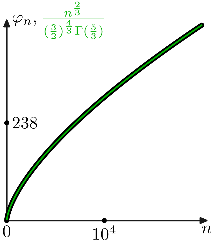
(a) First asymptotic term

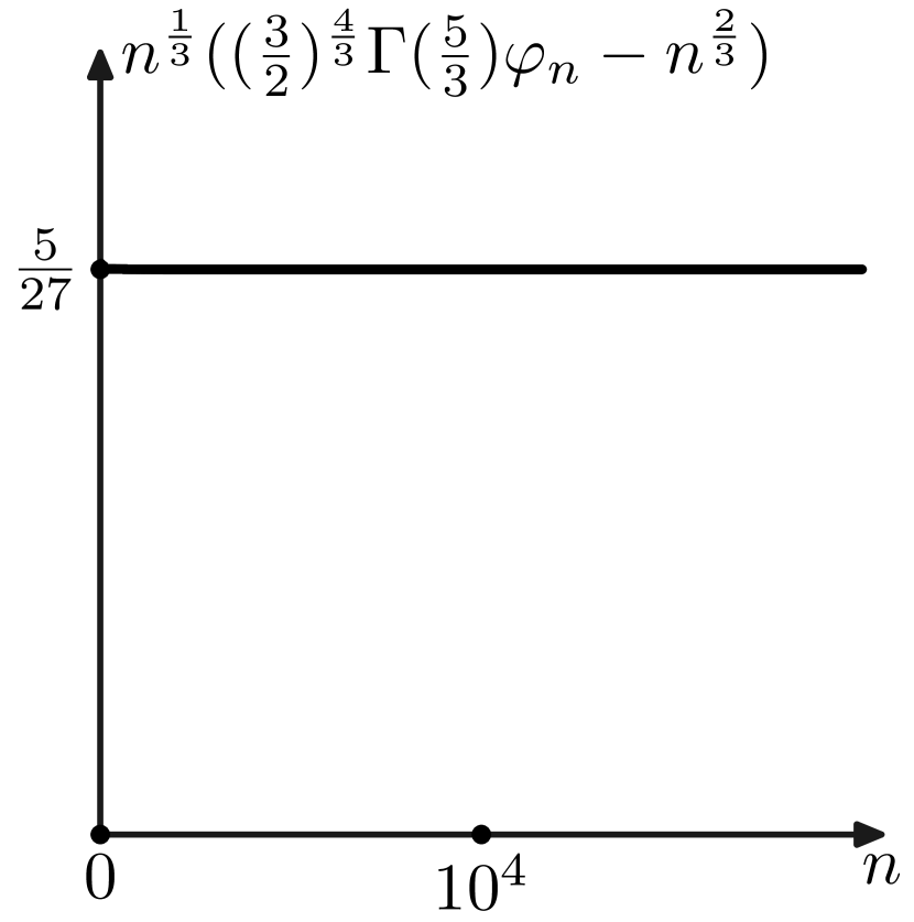
(b) Second asymptotic term

Figure 1: Plots show how good asymptotics (24) is.

3.3 Example 2.

The case $q(z)=z+z^{3}$. We have

$$b_{1}=1,\ \ b_{2}=\frac{-1-\sqrt{7}\mathbf{i}}{2},\ \ b_{3}=\frac{-1+\sqrt{7}\mathbf{i}}{2},\ \ q(1)=q(b_{1})=2,\ \ q^{\prime}(1)=q^{\prime}(b_{1})=4,\ \ q^{\prime\prime}(1)=6,$$

$$q^{\prime}(b_{2})=\frac{-7+3\sqrt{7}\mathbf{i}}{2},\ \ q^{\prime}(b_{3})=\frac{-7-3\sqrt{7}\mathbf{i}}{2}.$$

The explicit expression for $\varphi_{n}$, see (14), is

$$\varphi_{n}=\sum_{m_{2}=0}^{n-1}\sum_{m_{1}=m_{2}}^{n-1}\binom{-\frac{4}{3}}{m_{2}}(-1)^{m_{2}}\binom{\frac{-35+\sqrt{7}\mathbf{i}}{28}}{m_{1}-m_{2}}\biggl{(}\frac{-1+\sqrt{7}\mathbf{i}}{4}\biggr{)}^{m_{1}-m_{2}}\binom{\frac{-35-\sqrt{7}\mathbf{i}}{28}}{n-1-m_{1}}\biggl{(}\frac{-1-\sqrt{7}\mathbf{i}}{4}\biggr{)}^{n-1-m_{1}}.$$

The asymptotics for large $n$, see (15), is

$$\varphi_{n}\simeq\frac{2}{\sqrt{\pi}}\biggl{|}\biggl{(}\frac{5+\sqrt{7}\mathbf{i}}{4}\biggr{)}^{\frac{-35-\sqrt{7}\mathbf{i}}{28}}\biggr{|}^{2}\biggl{(}\sqrt{n}+\frac{5}{16\sqrt{n}}+...\biggr{)}.$$ (25)

Again, this asymptotic expansion is perfect enough as seen in Fig. 2.

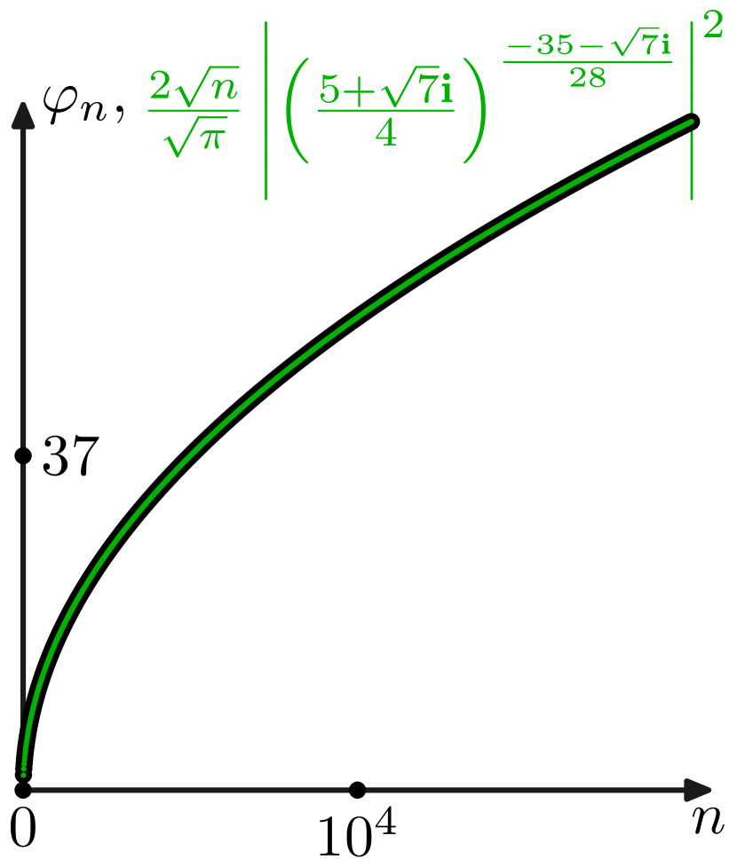
(a) First asymptotic term

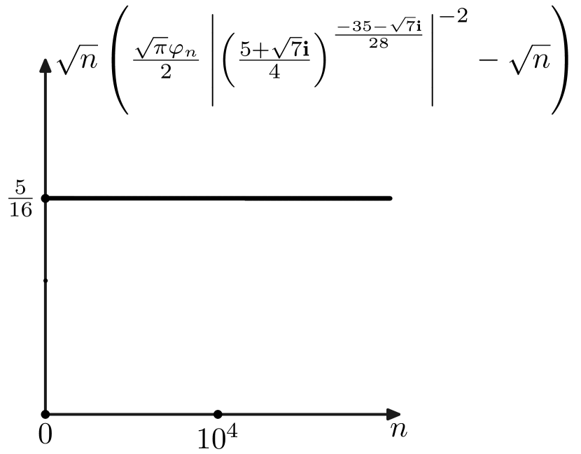
(b) Second asymptotic term

Figure 2: Plots show how good asymptotics (25) is.

3.4 Example 3.

Let us compare the cases of random environments with a Galton-Watson process in a constant environment. We take $q(z)=z$ considered in Example 0 and fix $r=1$. Then the generating function for the ratios of rare events $\Phi(z)$ satisfies the Schröder-type functional equation

$$\Phi(ze^{z-1})=e^{-1}\Phi(z),\ \ \Phi(0)=0,\ \ \Phi^{\prime}(0)=1,$$ (26)

see (10), where $r=1$ is fixed. Now, we will follow the ideas of [6] and mostly skip some details. No explicit solutions for (26) are known. It is not surprising, since this domain coincides with the filled Julia set for the exponential generating function and has a complex fractal form, see its approximate structure in Fig. 3(a).

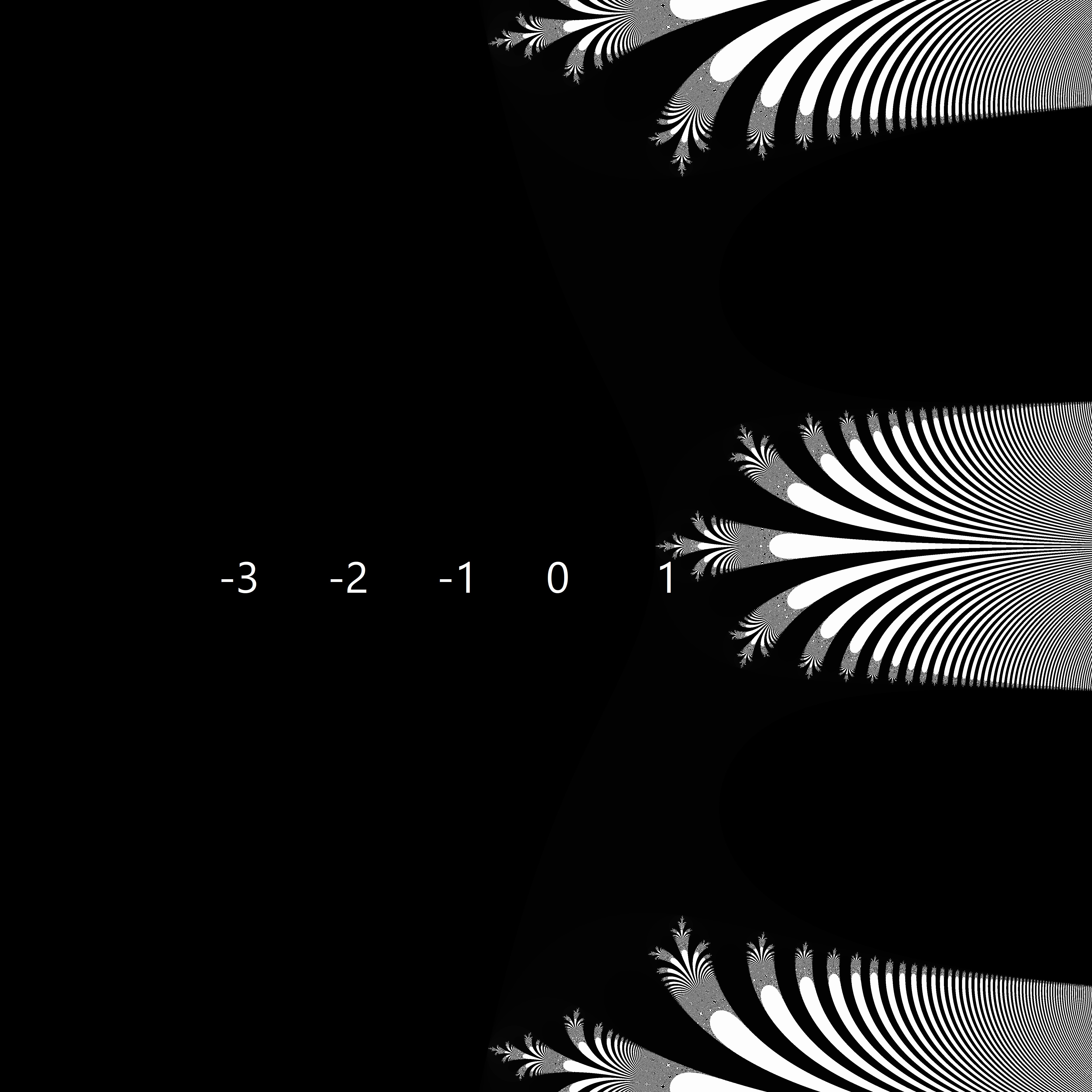
(a) Filled Julia set for $ze^{z-1}$

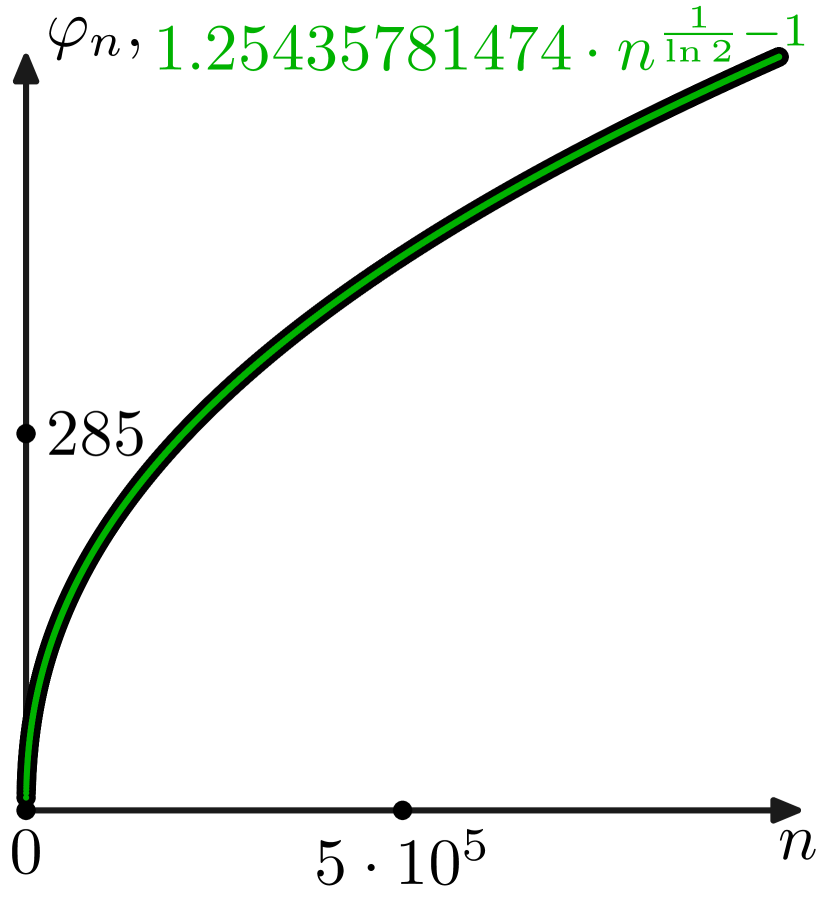
(b) Exact values and first asymptotic term

Figure 3: (a) The domain of definition (black area) of $\Phi(z)$, see (26), in complex plane ${\mathbb{C}}$; (b) Taylor coefficients of $\Phi(z)$ compared with its firs asymptotic term.

Using (26), we can write recurrence expression for determining $\varphi_{n}$ - Taylor coefficients of $\Phi(z)$ at $z=0$:

$$\varphi_{1}=1,\ \ \ \frac{\varphi_{n}}{e}=\frac{\varphi_{n}}{e^{n}}+\frac{(n-1)^{1}\varphi_{n-1}}{1!e^{n-1}}+\frac{(n-2)^{2}\varphi_{n-2}}{2!e^{n-2}}+...+\frac{\varphi_{1}}{(n-1)!e},\ n>1.$$

Moreover, results of [6] allow us to write an approximate expression

$$\varphi_{n}\approx 1.25435781474...n^{{\frac{1}{\ln 2}}-1},$$ (27)

where the constant is an average value of the so-called Karlin-MacGregor function related to $ze^{z-1}$, the approximation is quite good, see Fig. 3(b). However, in contrast to the examples of random environments, no explicit expressions through known constants exist. Moreover, apart from the constant term multiplied by the power of $n$, the first asymptotic term also contains small oscillatory elements, see Fig. 4. The presence of oscillations is the significant difference between constant and random environments. Note that, if we take averaging not over the entire interval $(0,+\infty)$ in (10), but only over part of it, then the oscillations in the first asymptotic term will disappear, but will remain in the following terms of the asymptotics, as it is discussed in [7].

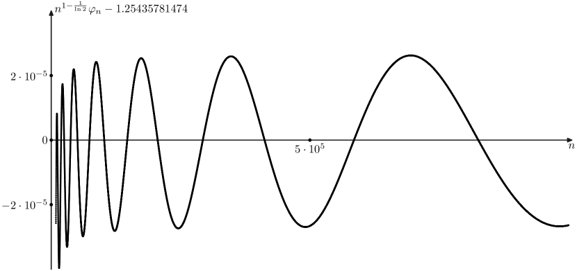
Figure 4: Oscillatory factors in the first asymptotic term for $\varphi_{n}$, see (27).

3.5 Example 4.

Let us compare the cases considered above with a process in a random environment averaged on an incomplete interval. We take $q(z)=z$ th same as in Example 0 and fix interval $r\in(2,+\infty)$ instead of $(0,+\infty)$. Then the generating function for the ratios of rare events $\Phi(z)$ satisfies the Schröder-type functional equation

$$\int_{2}^{+\infty}\Phi(ze^{r(z-1)})dr=e^{-2}\Phi(z),\ \ \Phi(0)=0,\ \ \Phi^{\prime}(0)=1,$$

or

$$\int_{0}^{ze^{2(z-1)}}\frac{\Phi(w)}{w}dw=e^{-2}(1-z)\Phi(z),\ \ \Phi(0)=0,\ \ \Phi^{\prime}(0)=1,$$ (28)

after the change of variable similar to (18). Identity (28) leads to the explicit recurrence relation for determining Taylor coefficients $\varphi_{n}$:

$$\varphi_{1}=1,\ \ \ \frac{\varphi_{n}-\varphi_{n-1}}{e^{2}}=\frac{\varphi_{n}}{ne^{2n}}+\frac{2(n-1)\varphi_{n-1}}{1!(n-1)e^{2(n-1)}}+\frac{2^{2}(n-2)^{2}\varphi_{n-2}}{2!(n-2)e^{2(n-2)}}+...+\frac{2^{n-1}\varphi_{1}}{(n-1)!e^{2}},\ n>1.$$

We follow the ideas explained in [7] to find approximations of $\varphi_{n}$ for large $n$. First of all, substituting linear combinations of $(1-z)^{\alpha}$ into (28), we find approximation of $\Phi(z)$ at $z=1$, namely

$$\Phi(z)\simeq c\biggl{(}(1-z)^{\alpha}+\frac{(4\alpha-1)(\alpha+1)}{3(2\alpha+1)}(1-z)^{\alpha+1}\biggr{)}+\mathop{\mathrm{Re}}\nolimits(b(1-z)^{\alpha_{1}})+...,$$ (29)

where

$$\alpha=-2.469874943242969...,\ \ \alpha_{1}=-1.469486150158083...\pm{\bf i}4.38645551777719...$$ (30)

are first roots with minimal real parts of the equation

$$\frac{-1-\alpha}{e^{2}}=3^{\alpha+1}.$$

Applying (19) and (21) to (29), we obtain the asymptotic expansion of $\varphi_{n}$:

$$\varphi_{n}\simeq C(n^{-\alpha-1}+C_{1}n^{-\alpha-2})+n^{-\mathop{\mathrm{Re}}\nolimits(\alpha_{1})-1}(B_{1}\cos(\mathop{\mathrm{Im}}\nolimits(\alpha_{2})\ln n)+B_{2}\sin(\mathop{\mathrm{Im}}\nolimits(\alpha_{2})\ln n))+...,$$ (31)

$$C_{1}:=\frac{(1+\alpha)(1-2\alpha)(2+\alpha)}{6(1+2\alpha)}.$$ (32)

In contrast to the first Examples, we have no fast algorithms for the computation of $C$, $B_{1}$, and $B_{2}$. There is an approximate value

$$C=1.281889848285....$$ (33)

The approximation (31) is quite good, see Figs. 5 and 6. Note that the oscillations in Fig. 5(b) attenuate slowly since the difference between $-\mathop{\mathrm{Re}}\nolimits(\alpha_{1})-1$ and $-\alpha-2$ is quite small. The significant difference with the standard Galton-Watson process in Example 3 is the absence of oscillations in the leading asymptotic term. However, the oscillations appear in the next term - this is the difference with the averaging over complete intervals considered in Examples 0, 1, and 2. We’ll leave an intriguing question to interested readers: What happens with oscillations if we average over $(1,+\infty)$ instead of $(2,+\infty)$?

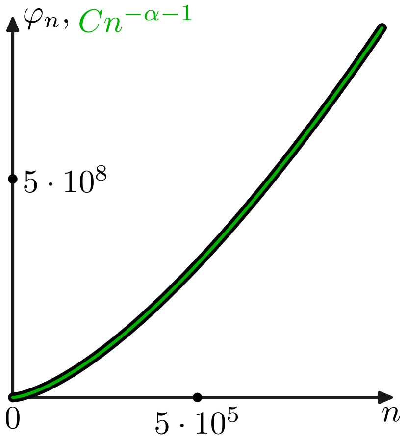
(a) Exact values and first asymptotic term

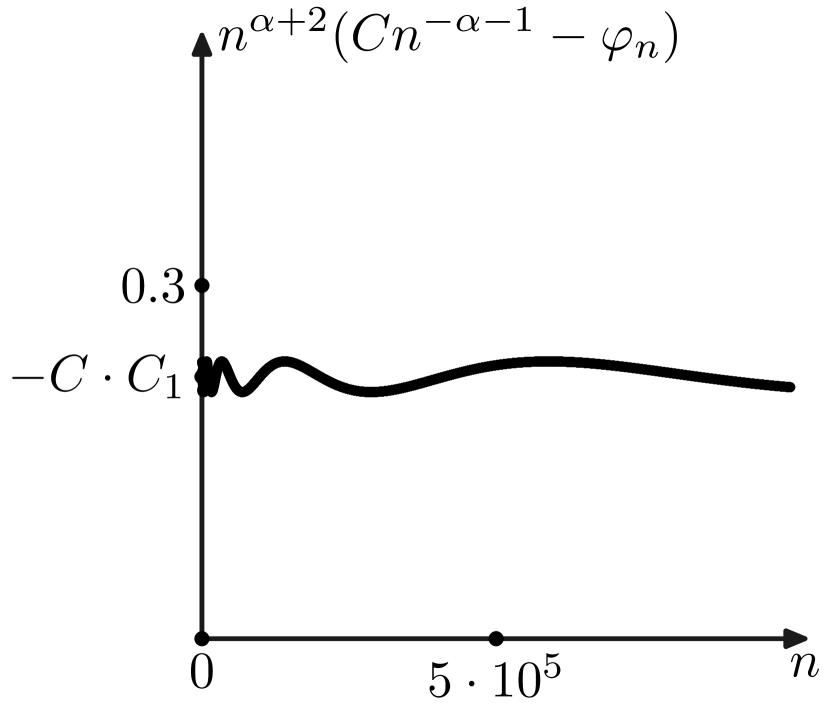
(b) Difference between exact values and first asymptotic term

Figure 5: Comparison between $\varphi_{n}$ and its asymptotics for Example 4.

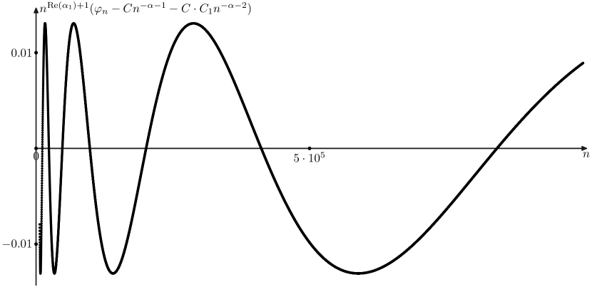
Figure 6: Oscillatory factors in the second asymptotic term for $\varphi_{n}$, see (31).

3.6 Example 5.

As a bonus, let us consider the extended Bernoulli process in random environments with the probability-generating function

$$P_{r}(z)=z(r+(1-r)z)^{m},$$ (34)

where $m\in{\mathbb{N}}$. The parameter $r$ is uniformly distributed in the interval $(0,1)$. Then the generalized Schröder type integral-functional equation, see (4), is

$$\int_{0}^{1}\Phi(z(r+(1-r)z)^{m})dr=\frac{\Phi(z)}{m+1},\ \ \Phi(0)=0,\ \ \Phi^{\prime}(0)=1.$$ (35)

We will follow the ideas presented in Example 2 of [7], sometimes omitting details. Changing the variable $w=z(r+(1-r)z)^{m}$, we rewrite (35) as

$$\int_{z^{m+1}}^{z}\Phi(w)w^{\frac{1}{m}-1}dw=\frac{m}{m+1}(1-z)z^{\frac{1}{m}}\Phi(z).$$ (36)

Introducing

$$F(z)=\int_{0}^{z}\Phi(w)w^{\frac{1}{m}-1}dw,$$ (37)

we rewrite (36) as

$$\frac{F(z)-F(z^{m+1})}{z-z^{2}}=\frac{m}{m+1}F^{\prime}(z).$$ (38)

Equations (37) and (38) leads to recurrence formula for determining Taylor coefficients $\varphi_{n}$ of $\Phi(z)$:

$$\varphi_{1}=1,\ \ \ \varphi_{n}=\begin{cases}\frac{mn+1}{m(n-1)}\varphi_{n-1},&m+1\nmid n-1,\\ \frac{mn+1}{m(n-1)}\varphi_{n-1}-\frac{(m+1)^{2}}{m(n-1)}\varphi_{\frac{n-1}{m+1}}.&otherwise\end{cases},\ n>1.$$ (39)

Substituting ansatz $F(z)\simeq C(1-z)^{\alpha}$, $z\to 1$ into (38), we obtain equation for $\alpha$:

$$(m+1)^{\alpha}-1=\frac{m\alpha}{m+1}.$$ (40)

The solution of (40) with a minimal real part is $\alpha=-1$. This observation and (37) leads to $\Phi(z)\simeq C(1-z)^{-2}+...$ for $z\to 1$ and, hence, we obtain the approximation

$$\varphi_{n}\simeq Cn+....$$ (41)

On the other hand $F(z)\sim z^{1+\frac{1}{m}}/(1+1/m)$ for $z\to 0$ as it is seen from (37). These two asymptotic of $F(z)$ for $z\to 0$ and $z\to 1$ guess us the following definition

$$H(z)=\frac{(1-z)F(z)}{z^{1+\frac{1}{m}}},$$ (42)

for determining $C$, which satisfies

$$H(0)=\frac{m}{m+1},\ \ \ H(1)=C.$$ (43)

Definition (42) allows us to write (38) as

$$-\frac{(m+1)H(z^{m+1})z^{m}(1-z)}{1-z^{m+1}}=m(1-z)H^{\prime}(z)-H(z)$$ (44)

or

$$-\frac{(m+1)H(z^{m+1})z^{m}(1-z)^{\frac{1}{m}}}{1-z^{m+1}}=m(1-z)^{\frac{1}{m}}H^{\prime}(z)-(1-z)^{\frac{1}{m}-1}H(z),$$ (45)

which is

$$-\frac{(m+1)H(z^{m+1})z^{m}(1-z)^{\frac{1}{m}}}{1-z^{m+1}}=(m(1-z)^{\frac{1}{m}}H(z))^{\prime}.$$ (46)

After integration (46) becomes

$$H(z)=\frac{(1-z)^{-\frac{1}{m}}}{m}\int_{z}^{1}\frac{(m+1)H(\zeta^{m+1})\zeta^{m}(1-\zeta)^{\frac{1}{m}}}{1-\zeta^{m+1}}d\zeta.$$ (47)

Now, this is an exciting moment - using (47) with the integration by parts yields

$$\int_{0}^{w}\frac{H(z)}{1-z}dz=\int_{0}^{w}\frac{(1-z)^{-1-\frac{1}{m}}dz}{m}\int_{z}^{1}\frac{(m+1)H(\zeta^{m+1})\zeta^{m}(1-\zeta)^{\frac{1}{m}}}{1-\zeta^{m+1}}d\zeta=\\ (1-z)^{-\frac{1}{m}}\int_{z}^{1}\frac{(m+1)H(\zeta^{m+1})\zeta^{m}(1-\zeta)^{\frac{1}{m}}}{1-\zeta^{m+1}}d\zeta\biggl{|}_{z=0}^{w}+\int_{0}^{w}\frac{(m+1)H(\zeta^{m+1})\zeta^{m}}{1-\zeta^{m+1}}d\zeta,$$ (48)

which with (47) gives

$$\int_{w^{m+1}}^{w}\frac{H(z)}{1-z}dz=m(H(w)-H(0)).$$ (49)

When $w\to 1$, (49) leads to

$$H(1)\ln(m+1)=m(H(1)-H(0)),$$ (50)

which, see (43), gives

$$C=\frac{m^{2}}{(m+1)(m-\ln(m+1))}.$$ (51)

Thus, by (41), we have

$$\varphi_{n}=\frac{m^{2}n}{(m+1)(m-\ln(m+1))}+...,\ \ n\to+\infty.$$ (52)

Example $m=1$ is already considered in [7]. For $m=2$, the comparison of exact values $\varphi_{n}$, computed by (39), and its asymptotic (52) is provided in Fig. 7. The linear growth of $\varphi_{n}$ is confirmed by its asymptotics (52). The second asymptotic term is provided in Fig. 7(b). This is a bounded sequence of period $3$. Using ideas from [7], it is possible to write the values of this sequence explicitly. This is a very fun exercise for interested readers.

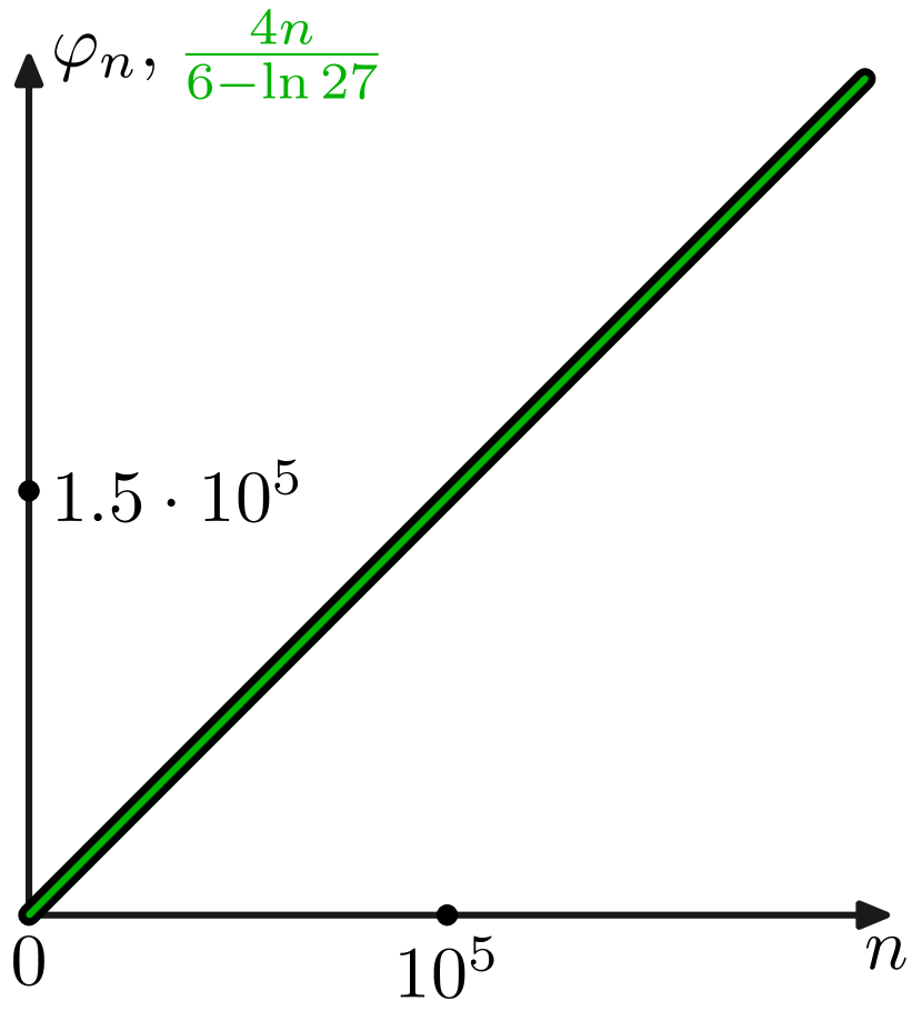
(a) Exact values and first asymptotic term

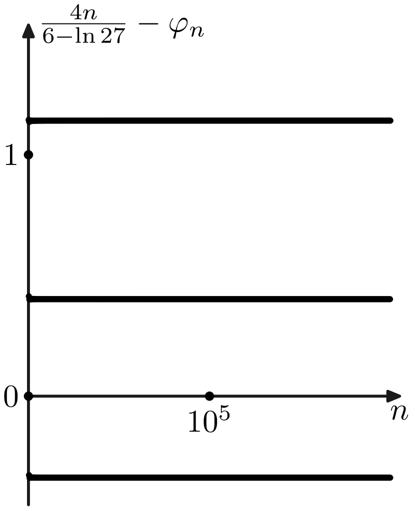
(b) Difference between exact values and first asymptotic term

Figure 7: Comparison between $\varphi_{n}$ and its asymptotics for Example 5, see (52), where $r=2$.

References

- [1] J. D. Biggings and N. H. Bingham, “Near-constancy phenomena in branching processes”. Math. Proc. Cambridge Phil. Soc., 110, 545-558, 1991.
- [2] B. Derrida, C. Itzykson, and J. M. Luck, “Oscillatory critical amplitudes in hierarchical models”. Comm. Math. Phys., 94, 115–132, 1984.
- [3] O. Costin and G. Giacomin, “Oscillatory critical amplitudes in hierarchical models and the Harris function of branching processes”. J. Stat. Phys., 150, 471–486, 2013.
- [4] B. Derrida, S. C. Manrubia, D. H. Zanette. “Distribution of repetitions of ancestors in genealogical trees”. Physica A, 281, 1-16, 2000.
- [5] J. E. Cohen and T. E. Huillet, “Taylor’s law for some infinitely divisible probability distributions from population models”. J. Stat. Phys., 188, 33, 2022.
- [6] A. A. Kutsenko, “Approximation of the number of descendants in branching processes”. J. Stat. Phys., 190, 68, 2023.
- [7] A. A. Kutsenko, “Generalized Schröder-type functional equations for Galton-Watson processes in random environments”. https://arxiv.org/abs/2309.13765, 2024.
- [8] T. E. Harris, “Branching processes”, Ann. Math. Statist., 41, 474-494, 1948.
- [9] N. H. Bingham, “On the limit of a supercritical branching process”. J. Appl. Probab., 25, 215–228, 1988.
- [10] B. Bollobás, S. Janson, and O. Riordan, “Sparse random graphs with clustering”. Random Struct. Algor., 38, 269-323, 2011.
- [11] S. Portnoy, “Edgeworth’s time series model: Not AR(1) but same covariance structure”. J. Econom., 213, 281–288, 2019.
- [12] F. Tricomi and A. Erdélyi, “The asymptotic expansion of a ratio of Gamma functions”. Pac. J. Math., 1, 133–142, 1951.