Dynamic programming principle in cost-efficient sequential design: application to switching measurements

Abstract

We study sequential cost-efficient design in a situation where each update of covariates involves a fixed time cost typically considerable compared to a single measurement time. The problem arises from parameter estimation in switching measurements on superconducting Josephson junctions which are components needed in quantum computers and other superconducting electronics. In switching measurements, a sequence of current pulses is applied to the junction and a binary voltage response is observed. The measurement requires a very low temperature that can be kept stable only for a relatively short time, and therefore it is essential to use an efficient design. We use the dynamic programming principle from the mathematical theory of optimal control to solve the optimal update times. Our simulations demonstrate the cost-efficiency compared to the previously used methods.

Keywords: optimal design, D-optimality, complementary log-log link, Josephson junction

1 Introduction

We study an optimal design problem motivated by switching measurements in quantum physics. In these measurements, a Josephson junction (JJ) [8], an important nonlinear component in superconducting electronics utilized for example in quantum computers [11], is placed at a temperature close to absolute zero to obtain superconductivity. When a current pulse is applied to the junction, a voltage pulse is observed with a probability that depends on the height of the current pulse. The relation between the height of the current pulse and the probability of the voltage pulse can be accurately approximated by a binary response model with a complementary log-log link [10]. The unknown model parameters $a$ and $b$ determine the slope and the location of the response curve and depend on the physical dimensions of the junction. The problem is to choose the covariate values, i.e., the height of the applied current pulse in our case, in order to estimate the parameters of interest in the most efficient manner in the sense of D-optimality (see Section 2). Efficiency is essential because in switching measurements, the required temperature can be kept stable only for a relatively short time.

Sequential experimentation provides benefits over static designs. In nonlinear models, the optimal design depends on the parameters. As the true values of the parameters are unknown, the optimality properties of a design depend on the accuracy of initial estimates of the parameters. A sequential design allows us to update the estimates after each new observation and thus improve the design. In practice, sequential experimentation has its price. In switching measurements, adjusting the pulse generator to change the covariate values takes a time that is considerably larger than the time needed for a single measurement. This leads to cost-efficiency considerations where one must balance the cost of an update and the information obtained from it. The sequential design is then replaced by a batch-sequential design, and the key problem is determining the optimal update times.

The batch-sequential design problem in the context of switching measurements was formulated by Karvanen, Vartiainen, Timofeev and Pekola [10]. They implemented an ad hoc method that increased the number of measurements by 10 % at each stage. Later in [9], an approximate asymptotic model for accumulation of a quantity approximating the D-criterion was presented. Moreover, an ad hoc method for solving the optimal update times was implemented. The purpose of the current paper is in the context of the approximate asymptotic model to solve the optimal update times in a precise manner using the mathematical theory of optimal control, and the dynamic programming principle (DPP) in particular.

The DPP roughly speaking means that instead of considering a process until the end we look at the problem over one step or stage. A simple example is given by a random walk where we jump left or right each with probability $1/2$ on the integers $\{1,2,\ldots,9\}$ and stop if we reach $0$ or $10$ where we get some given payoff. When looking at the expectation in this process when starting at $x_{0}$ (denoted by $u(x_{0})$), the DPP for the expectation reads as

$$u(x_{0})={\frac{1}{2}}\big{(}u(x_{0}-1)+u(x_{0}+1)\big{)}.$$

In other words, this says that the expectation at a point can be considered by looking at one step and summing up the outcomes with the corresponding probabilities: we either go left with probability $1/2$ or right with probability $1/2$ and take the expectations from there. More examples can be found for example in [6, Section 10.3], [2] or [14, Chapter 1]. In the design of experiments, dynamic programming has been applied to sequential experimentation with linear models [3].

The key dynamic programming equations in our case are formulated in Sections 3.1 and 3.2. From these, we then solve the optimal update times using R [15]. In particular, we take into account which target (time or optimal accumulated $D$) we are optimizing, and present the method to solve both of these problems. Moreover, the dynamic programming principles automatically take into account the amount of information we have obtained during the initialization and the update cost when determining the optimal update times.

In Section 4, we present the results obtained through a simulation testing the DPP method and previous methods in the literature. The results show that the suggested method is more cost efficient. Finally, we remark that the use of optimal control should find a wide variety of applications in cost-efficient sequential designs with different statistical models. It is by no means limited to the presented examples.

2 Preliminaries: $D$-optimal designs for complementary log-log regression

In this paper, we deal with the DPP in the context of $D$-optimal designs, where D is the determinant or equivalently the square root of the determinant of the information matrix. The preliminaries of the DPP are given in the appendix and the next section: before we can write down the DPP we need to recall the basic notation for the $D$-optimal design. The process of deriving the (locally) $D$-optimal design involves maximizing the criterion $D$ under certain assumptions, in particular assuming knowledge of the true parameter values. A detailed exposition of this derivation in a generalized form is presented in [7]. Moreover, the extensively employed logit model has been explored in various works, including studies by [1], [13], [16], as well as [12]. These references collectively demonstrate that the $D$-optimal design represents a two-point design applicable to logit, probit, and cloglog models, enabling the determination of optimal covariate values. Additionally, extensions addressing models involving multiple covariates have been investigated by [17], [5], and [4].

Here we consider an experiment, where our task is to estimate the unknown parameters $\bm{\theta}=(a,b)$. We assume that the binary random variable is distributed according to

$$P(Y=1|\bm{\theta})=1-e^{-\exp(ax+b)},$$

$$P(Y=0|\bm{\theta})=e^{-\exp(ax+b)},$$ (2.1)

where $x$ is the covariate.

The task is to select the covariate values $x_{1},\ldots,x_{n}$ in such a way that the parameters can be estimated from the observed data $y_{1},\ldots,y_{n}$ as efficiently as possible. Starting from (2) the likelihood reads for independent observations as

$$L(\bm{y}|\bm{\theta}) :=\prod_{i=1}^{n}P(Y=y_{i}|\bm{\theta})$$

$$:=\prod_{i=1}^{n}\Big{\{}y_{i}(1-e^{-\exp(ax_{i}+b)})+(1-y_{i})e^{-\exp(ax_{i}+b)}\Big{\}}.$$

Thus the log-likelihood is

$$l(\bm{\theta}): =\sum_{i=1}^{n}\log P(Y=y_{i}|\bm{\theta})$$

$$=\sum_{i=1}^{n}\Big{\{}y_{i}\log((1-e^{-\exp(ax_{i}+b)}))-(1-y_{i})\exp(ax_{i}+b)\Big{\}}.$$ (2.2)

The Fisher information matrix is defined to be

$$J=-{\mathbb{E}\,}\begin{pmatrix}\frac{\partial^{2}l}{\partial a^{2}}&\frac{\partial^{2}l}{\partial a\partial b}\\ \frac{\partial^{2}l}{\partial b\partial a}&\frac{\partial^{2}l}{\partial b^{2}}\end{pmatrix},$$

assuming that we know $a$ and $b$ in order to compute the expectation. Observe that the Fisher information depends on the sample size but not on the measurements $y_{i}$. Heuristically speaking, the Fisher information measures the curvature of the graph of log-likelihood and thus tells how stable the maximum likelihood estimate is.

Computing the Fisher information, we get

$$J=\begin{pmatrix}\sum_{i=1}^{n}g(z_{i})x_{i}^{2}&\sum_{i=1}^{n}g(z_{i})x_{i}\\ \sum_{i=1}^{n}g(z_{i})x_{i}&\sum_{i=1}^{n}g(z_{i})\end{pmatrix}$$

where $z_{i}=ax_{i}+b$ and

$$g(z)=\frac{e^{2z}}{e^{\exp(z)}-1}.$$

We formulate the $D$-citerion in terms of

$$D:=\sqrt{\det(J)}.$$

In D-optimal design, our task is to find $x_{1},\ldots,x_{n}$ so that $D$ (or equivalently $D^{2}$) is maximized. Here we selected the square root instead of the determinant in order to have correct scaling properties later on. By re-organizing the terms, we obtain

$$D^{2}:=\det(J) =\sum_{i=1}^{n}g(z_{i})x_{i}^{2}\sum_{i=1}^{n}g(z_{i})-\Big{(}\sum_{i=1}^{n}g(z_{i})x_{i}\Big{)}^{2}$$

$$=\sum_{i=1}^{n-1}\sum_{j=i+1}^{n}g(z_{i})g(z_{j})(x_{i}-x_{j})^{2}.$$

The D-optimal design is a two-point design and we can maximize

$$D^{2}=\det(J)=\frac{1}{a^{2}}g(z_{1})g(z_{2})(z_{1}-z_{2})^{2}$$

to obtain the values

$$(z_{1}^{*},z_{2}^{*})=(0.97963269129,-1.337736677)$$

as well as $(z_{1}^{*},z_{2}^{*})=(-1.337736677,0.97963269129)$ [7]. The Fisher information matrix corresponding to these values is denoted by $J^{*}$. In other words, $J^{*}$ is the information matrix for $D$-optimal covariates when $n=2$.

We use the approximation from [9] for the expected change in $D$ when two additional measurements are made. Our intention here is not to study the model there, but rather show, given such a model, how to solve the optimal update times using the dynamic programming principle. In any case, we briefly recall the setting in [9]. Similarly as there, for now, we assume that $(a,b)=(1,0)$ and only comment on the other cases later. We set

$$J^{*} =\sum_{i=1}^{2}g(z^{*}_{i})\begin{pmatrix}(x^{*}_{i})^{2}&x^{*}_{i}\\ x^{*}_{i}&1\end{pmatrix},$$

where $z^{*}_{i}=ax^{*}_{i}+b=x^{*}_{i}$, and observe that $\sqrt{\det(J^{*})}=0.80940268$. Motivated by the asymptotic normality of maximum likelihood estimates it was assumed that $\hat{a}$ and $\hat{b}$ are normally distributed with the mean $(a,b)$ and with the covariance matrix $J^{-1}(D)$, where $J(D)$ represents the accumulated information. Then in the simulation pairs $(\hat{a},\hat{b})$ were generated from the distribution $N((1,0),J^{-1}(D))$, and for each simulated $(\hat{a},\hat{b})$, the following quantity was computed:

$$\det\Bigg{(}\sum_{i=1}^{2}g(z_{i})\begin{pmatrix}x_{i}^{2}&x_{i}\\ x_{i}&1\end{pmatrix}\Bigg{)}^{1/2} =\sqrt{g(z_{1})g(z_{2})}(z_{1}-z_{2}),$$

where

$$z_{1} =\frac{z_{1}^{*}-\hat{b}}{\hat{a}},\quad\quad z_{2}=\frac{z_{2}^{*}-\hat{b}}{\hat{a}}.$$

The expected change in $D$ was taken to be the average of these simulated quantities. Since the model is founded on such an accumulation property that holds asymptotically (similarly to the previous steps) we give a brief justification for it in Appendix A. The expected change given by the simulation in [9] was

$$h(D)=\frac{0.80940268}{1+e^{\eta+\theta\log(D)}},$$ (2.3)

where $\eta=1.88938,\ \theta=-1.51330$. Since $\lim_{D\to 0+}h(D)=0$ we also need an initialization procedure that gives us the initial $D_{0}>0$ and the first MLE to get started.

3 Optimal update times

Given the model described in the previous section, we now show how to solve optimal update times using dynamic programming. We consider two problem settings: given the available time, we want to maximize the accumulated $D$, or given the desired $D$, we want to minimize the time used to reach this target. The dynamic programming principles below can easily be solved numerically by iterating backwards from the final condition.

3.1 Given final time, maximize the accumulated $D$

We consider a situation where the termination time $T$ is given, and we want to maximize the accumulated $D$. For example, it is known that the Josephson junction remains at a required temperature and thus is stable for a certain time $T$. Time cost $C_{s}$ for updating the covariate is assumed to be a nonnegative integer and is here usually large compared to the cost of a single measurement (the cost of the single measurement is scaled to be 1). For example, $C_{s}$ could be the time cost for adjusting the current in the pulse generator. The task is to find the optimal update times so as to accumulate as large $D$ as possible by the termination time $T$. The problem is to decide the next update time at the current update time $t$ assuming that the accumulated $D\geq D_{0}>0$ is given. Let us denote by

$u(D,t)$, amount of $D$ we can optimally accumulate during the rest of the experiment if starting at $(D,t)$ and updating immediately.

This description is enough for now, but the precise definition is given in Appendix B. Using the terminology from the control theory, the value function $u$ satisfies the DPP with $C_{s}>0$ and $t<T-C_{s}$

$$u(D,t) =\sup_{t_{\text{next}}\in(t+C_{s},T]\cap{\mathbb{Z}}_{+}}\Big{\{}u(D_{\text{next}},t_{\text{next}})+(D_{\text{next}}-D)\Big{\}},$$ (3.4)

where

$$t,C_{s} \in{\mathbb{Z}}_{+},\ {\mathbb{Z}}_{+}=\{0,1,2,\ldots\},$$

$$D_{\text{next}}: =D_{\text{next}}(t_{\text{next}},D):=D+h(D)(t_{\text{next}}-t-C_{s}),$$

$$u(D,t) =0,\quad t\in[T-C_{s},T]\cap{\mathbb{Z}}_{+}.$$

What the DPP says is that we can compute the optimal value at a point, by taking one optimal stage of measurements and the optimal value from where we ended up during this one stage.

Also observe that it does not matter that it was assumed that $a=1$ in $h$ since everything would be just scaled by the true value of $a$, and this does not affect the update times. However, inside the DPP, the quantity $D$ corresponds to $a=1$ and should not be taken as an approximation of the ’true $D$’. Nonetheless, the observed $D$ can easily be computed from the sample.

We will solve for $u$ starting from $t=T-C_{s}-1$. When at $(D,t)$, supposing that we have already solved values $u$ for all $s>t$, we may solve for $u(D,t)$, using (3.4). In the course of using (3.4), we also solve and save the stage update times for each $D$. Then we pick the stage update time $t_{next}$ for $(D,t)=(D_{0},0)$, and by continuing, for the rest of the stages. Figure 1 gives two examples.

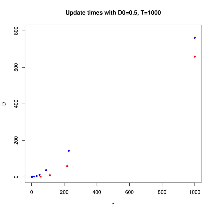
(a) Fixed $D_{0}$ case ($D_{0}=0.5$)

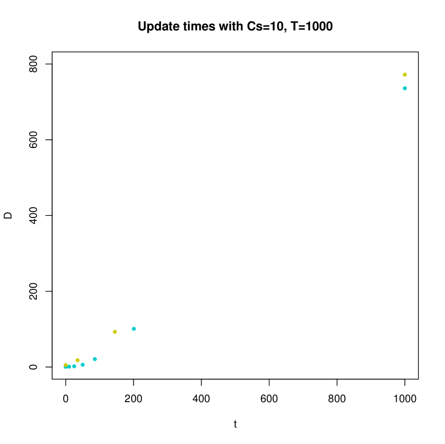
(b) Fixed $C_{s}$ case ($C_{s}=10$)

Figure 1: Update times with $T=1000$ (the point $T=1000$ is not an update time but shows the final accumulated $D$). The left subfigure indicates the update times for fixed $D_{0}=0.5$ ($C_{s}=5$ in blue, $C_{s}=30$ in red). The right one represents those times for fixed $C_{s}=10$ ($D_{0}=0.5$ in cyan, $D_{0}=5$ in yellow).

The optimization is implemented in the R codes available at optimaltimesCsA.r and optimaltimesCsB.r. In these R-codes, for example, optimaltimesCs.r, we have discrete grids for $D_{i},\ i=1,\ldots,N_{D}$ and $t_{j},\ j=1,\ldots,N_{T}$. When at a point $(D_{i_{0}},t_{j_{0}})$, we consider the time points $\tilde{t}_{j}\in\{\tilde{t}_{1},\ldots,\tilde{t}_{N_{t_{j_{0}}}}\}:=\{t_{j_{0}}+C_{s},\ldots,t_{N_{T}}=T\}$ and compute the values

$$\tilde{D}_{\tilde{t}_{j}}:=D_{k}+h(D_{k})(\tilde{t}_{j}-t_{j_{0}}-C_{s}).$$

On the other hand, we have already computed all the future values for $u$ at the discretized values of $D_{i},\ i=1,\ldots,N_{D}$. Thus rounding $\tilde{D}_{t_{j}}$ to the nearest grid value $D_{k}$, we know $u(D_{k},\tilde{t}_{j})$ and we may form

$$DPP_{i_{0},j}:=u(D_{k},\tilde{t}_{j})+(\tilde{D}_{\tilde{t}_{j}}-D_{i_{0}}),\quad\text{for all}\quad j=1,\ldots,N_{t_{j_{0}}}.$$

Now, according to (3.4), we have solved the values of $u$ at time $t_{j_{0}}$. Then we continue to time $t_{j_{0}}-1$.

3.2 Given desired $D_{\text{final}}$, minimize the time cost

In this section, we consider a different problem where the goal is to reach a given final value of accuracy $D_{\text{final}}$ in the shortest possible time. Let us denote by

$v(D)$, the minimal time to reach $D_{\text{final}}$ if we update immediately.

Again for a more detailed discussion, see Appendix B. First, as indicated above, we observe that $v$ does not depend on the time spent so far since we only look at the future accumulation of $D$. We still denote the change of $D$ in one double measurement by $h(D)$ given in (2.3), and by $C_{s}\in{\mathbb{Z}}_{+}$ the update cost of the covariates. Now $v$ satisfies the following DPP

$$v(D) =\inf_{\Delta t\in(C_{s},\infty)\cap{\mathbb{Z}}_{+}}\Big{\{}v\big{(}D+(\Delta t-C_{s})h(D)\big{)}+\Delta t\Big{\}},$$ (3.5)

$$v(D) =0\quad\text{ for }\quad D\geq D_{\text{final}}.$$

Recall that we only applied $(a,b)=(1,0)$ in the previous subsection, since the accumulated information in the general case can be obtained by scaling everything by the factor $a^{-2}$ with the true value of $a$. One should observe that also in the above DPP $D$ and $D_{\text{final}}$ denote the rescaled versions with $(a,b)=(1,0)$ and should not be taken as an approximation of the ’true D’. Also, the updates should not be launched by the observed $D$ computed from the sample but by the time steps $\Delta t$ that will be stored while numerically solving for $v$.

To finish the section, observe that the optimal update times depend (as they should) on whether we are minimizing the time cost or maximizing $D$, what are the final values of $T$ or $D_{\text{final}}$, the update time cost $C_{s}$, and $D_{0}$ after the initialization. Thus it is not practical to give update times in a table, but they can be solved for different values by using the provided codes.

4 Benchmark

In preceding studies [10, 9], several types of batch-sequential $D$-optimal design methods were presented. They used the measurement data for a JJ circuit given in https://github.com/JuhaKarvanen/switching_measurements_design. Here we simulate the experiment from scratch. We also use less intense initialization with bad initial guesses of $a$ and $b$ to obtain a lower value for $D_{0}$ and it can be reproduced through the code initialdatagen.r for the case when the stage size is 100 in the first round under the assumption $(a,b)=(0.24,-61)$. This is in order to illustrate the difference of the methods more clearly (the lower $D_{0}$, the more important the updates as well as cost-efficient designs are). In the code simulation.r, we first solved the DPP problem (3.4) (given final time, optimize accumulated D) with $T=3500$ and $C_{S}=0.88167/0.00386\approx 228.4$ and then obtained the optimal update times under our setting. After that, we ran 100 simulations based on those update times. We also conducted the same number of simulations for the model suggested in [9] for comparison. The results are illustrated in Figure 2. As a technical remark, $D$ in the figure is the actual observed $D$ computed from the sample, not the ‘model $D$’ that appears for example in the DPPs and is obtained using $h(D)$ and rescaling $(a,b)=(1,0)$. What we observe is that the DPP method is more cost-efficient than the model in [9].

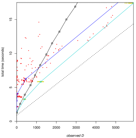
Figure 2: Simulations for three methods with $D_{0}=0.1408$ and $(a,b)=(0.24,-61)$. The black line marks the simulated results obtained in the same way as the ad hoc method used in the original experiment in [10]. The blue line and cyan line represent the time costs obtained by the approximate cost-efficient method in [9] and the DPP method of this paper, respectively. The blue and cyan squares represent the path with the corresponding experiment design calculated as the median of 100 simulated paths. The dots show the stages of the 100 simulated paths (red: [9] design, yellow: DPP design). The dashed line indicates the theoretical limit of the time cost if they are immediately measured at the optimal points. In the DPP design, we set $T=3500$ and the dotted line represents the total time cost (=17.42268 sec) in this case.

5 Discussion

We considered cost-efficient batch-sequential design in a situation where the update cost is large compared to the cost of a single measurement. The work was motivated by switching measurements of Josephson junctions. We made several improvements to the earlier literature: We formulated and solved a precise dynamic programming problem for update times if the change in $D$ is given by the function $h(D)$ obtained from the literature. In particular, the dynamic programming approach automatically takes into account which target (target time or target $D$) we are optimizing, and the effect of $D_{0}$, $C_{S}$ on update times. The simulations illustrate the efficiency of the proposed approach. Compared to earlier approximations [10, 9], a clear gain in cost-efficiency was seen.

However, there are still several approximations stemming from the earlier literature. The particular assumed form of the Fisher information in the simulation producing $h$, the normality assumption of MLE, and the assumed accumulation property of $D$, are such approximations and only hold asymptotically. The reason for these approximations is of course a desire to formulate the problem in such a way that it can be simulated and solved by efficient tools and in advance.

The proposed approach is directly applicable to switching measurements. In addition, a similar approach could be useful in other applications where the data are collected in batches and a cost is associated with each update. The functions $h(D)$ have been estimated also for the logit and probit link functions [9]. One might also want to consider the DPP approach with other optimality criteria.

Appendix A Accumulation of $D$ in the approximative model

To obtain an approximative model for the accumulation of $D$, the expected change in $D$ in [9] was taken to be the average of the simulated quantities $\sqrt{\det(J_{i})}$. Since the model is founded on such an accumulation property that holds asymptotically (similarly to the previous steps in the model) we give a brief justification for it here. To be more precise, we want to show in a suitable mode of stochastic convergence that

$$\sqrt{\det(J_{1}+\ldots+J_{n})}-\sqrt{\det(J_{1}+\ldots+J_{n-1})}-\sqrt{\det(J_{n})}\to 0$$ (1.6)

almost surely as $n\to\infty$, where $J_{i}=J_{i}(\omega)$ denotes the information obtained in the round $i$ for each sample $\omega$ (we use the notation $J_{i}$ for the convenience). In other words, the difference between the first two terms reflects the actual change in $D$ if we obtain the information $J_{n}$, and the last term the quantity used in the simulation. To establish the above asymptotic behaviour, let us denote $\Delta J_{i}:=(J_{i}-J^{*})$ and compute

$$\sqrt{\det(J_{1}+\ldots+J_{n})}=\det\Big{(}nJ^{*}+\sum_{i=1}^{n}\Delta J_{i}\Big{)}^{1/2}$$

$$=n\det\Big{(}J^{*}+\frac{1}{n}\sum_{i=1}^{n}\Delta J_{i}\Big{)}^{1/2}$$

$$=(n-1)\det\Big{(}J^{*}+\frac{1}{n}\sum_{i=1}^{n}\Delta J_{i}\Big{)}^{1/2}+\det\Big{(}J^{*}+\frac{1}{n}\sum_{i=1}^{n}\Delta J_{i}\Big{)}^{1/2}.$$

To get an approximation of

$$\sqrt{\det(J_{1}+\ldots+J_{n})}-\sqrt{\det(J_{1}+\ldots+J_{n-1})},$$

in order to prove (1.6) we also observe that

$$\sqrt{\det(J_{1}+\ldots+J_{n-1})}=(n-1)\det\Big{(}J^{*}+\frac{1}{n-1}\sum_{i=1}^{n-1}\Delta J_{i}\Big{)}^{1/2}$$

$$=(n-1)\det\Big{(}J^{*}+\frac{1}{n}\sum_{i=1}^{n}\Delta J_{i}$$

$$\hskip 70.0001pt+\frac{1}{n-1}\Big{(}\sum_{i=1}^{n-1}\Delta J_{i}-\sum_{i=1}^{n}\Delta J_{i}\Big{)}+\Big{(}\frac{1}{n-1}-\frac{1}{n}\Big{)}\sum_{i=1}^{n}\Delta J_{i}\Big{)}^{1/2}$$

$$=(n-1)\det\Big{(}J^{*}+\frac{1}{n}\sum_{i=1}^{n}\Delta J_{i}-\frac{1}{n-1}\Delta J_{n}+\frac{1}{n(n-1)}\sum_{i=1}^{n}\Delta J_{i}\Big{)}^{1/2}$$

$$=:(n-1)\det(A+B)^{1/2},$$

where the shorthand notation $A$ contains the first two terms and $B$ the last two terms. Also, observe that since we are working under the assumption $J_{i}\to J^{*}$ almost surely as $i\to\infty$, it holds that

$$(n-1)\det(B),\ (n-1)\operatorname{tr}(B)\to 0$$ (1.7)

almost surely as $n\to\infty$; we will need these facts later. Now we use a well-known formula for the determinant of a sum of $2\times 2$ matrices, and the mean value theorem or representation for the remainder term in Taylor’s theorem as in

$$\sqrt{x_{0}+h}=\sqrt{x_{0}}+(2c)^{-1/2}h,\text{ for some }c\text{ between }\text{$x_{0}$ and $x_{0}+h$}.$$

In this way

$$\det(A+B)^{1/2} =\big{(}\det(A)+\det(B)+\det(A)\operatorname{tr}(A^{-1}B)\big{)}^{1/2}$$

$$=\det(A)^{1/2}+(2c)^{-1/2}\big{(}\det(B)+\det(A)\operatorname{tr}(A^{-1}B)\big{)}.$$

Using this and (1.7), we get

$$(n-1) \bigg{(}\det\Big{(}J^{*}+\frac{1}{n}\sum_{i=1}^{n}\Delta J_{i}\Big{)}^{1/2}-\det\Big{(}J^{*}+\frac{1}{n-1}\sum_{i=1}^{n-1}\Delta J_{i}\Big{)}^{1/2}\bigg{)}$$

$$=(n-1)\bigg{(}\det(A)^{1/2}-\det(A+B)^{1/2}\big{)}$$

$$=-(n-1)(2c)^{-1/2}\big{(}\det(B)+\det(A)\operatorname{tr}(A^{-1}B)\big{)}\to 0,$$

almost surely as $n\to\infty$, since

$$\left|\operatorname{tr}(A^{-1}B)\right|\leq\left|\left|A^{-1}\right|\right|_{\infty}\operatorname{tr}(B).$$

Combining the above estimates, we deduce

$$\sqrt{\det(J_{1}+\ldots+J_{n})}-\sqrt{\det(J_{1}+\ldots+J_{n-1})}-\sqrt{\det(J_{n})}\to 0$$

almost surely when $n\to\infty$, as desired.

Appendix B Mathematical remarks on dynamic programming

In this section, we review part of the mathematical background for the optimal control problem in question, see for example [6, 2]. The literature is vast and it is impossible to give a thorough overview here.

B.1 Given final time, maximize the accumulated $D$ problem

Let $C_{s}>0$. The function $u:(0,\infty)\times[0,T]\to{\mathbb{R}}$ denotes the optimal amount $D$ we can accumulate during the remaining time if updating at the considered time. To be more precise, the controller chooses the update times

$${\mathbf{t}}:=(t_{0},\ldots,t_{n+1}),$$

where the difference between the update times is larger than $C_{s}$, and otherwise the number $n$ may vary. Also, observe that $t_{0}$ and $t_{n+1}$ must correspond to the interval we are considering. For example, if we consider the full interval, then $t_{0}=0$ and $t_{n+1}=T$, but this will be clear from the context. The definition of $u$ now reads as

$$u(D,t) =\begin{cases}\sup_{{\mathbf{t}}}\sum_{i=0}^{n}(t_{i+1}-t_{i}-C_{s})h(D(t_{i})),&t<T-C_{s}\\ 0,&t\in[T-C_{s},T],\end{cases}$$ (2.8)

where

$$D^{\prime}(s) =\begin{cases}h(D(t_{i})),&\text{ if }s\in[t_{i}+C_{s},t_{i+1}),\\ 0,&\text{ otherwise}.\end{cases}$$ (2.9)

Obviously, $u$ given by (2.8) exists and is unique.

Lemma B.1 (DPP)

Let $u$ be as in (2.8). Then for $C_{s}>0$ and $t<T-C_{s}$

$$u(D,t) =\sup_{t_{\text{next}}\in(t+C_{s},T]}\Big{\{}u(D_{\text{next}},t_{\text{next}})+(D_{\text{next}}-D)\Big{\}},$$ (2.10)

where

$$D_{\text{next}}: =D+h(D)(t_{\text{next}}-t-C_{s}).$$

The validity of the DPP can be readily verified by plugging in the definition (2.8). One could also study the DPP on its own right without invoking (2.8) and showing existence and uniqueness using a similar idea as in the numerical computation: since $C_{s}>0$, iterating backwards from the end $T$, we can extend the values to each strip of width $C_{s}$.

Remark B.2 (Regularity, stability of update times)

Similarly as in [6, Section 10.3], we can also prove that $u$ is bounded and Lipschitz continuous in $(0,\infty)\times[0,T]$. From the definition of $h$ and (2.8), it is straightforward that

$$u(D,t)\leq h^{\ast}(T-C_{s}),$$

where $h^{\ast}=\sqrt{\det(J^{*})}=0.80940268$ is the maximum value of $h$.

The basic idea in the proof of Lipschitz continuity is to ‘copy’ the update times from a nearby point of interest. We will show

$$|u(D,t)-u(\tilde{D},\tilde{t})|\leq C(|D-\tilde{D}|+|t-\tilde{t}|)$$

for some universal $C>0$ and any $(D,t),(\tilde{D},\tilde{t})\in(0,\infty)\times[0,T]$. We first estimate

$$|u(D,t)-u(\tilde{D},t)|$$

and without loss of generality we may assume that $\tilde{D}\geq D$ and $u(\tilde{D},t)\geq u(D,t)$. To this end, for $t\in[0,T]$, we can choose update times $\mathbf{t}_{1}=(t_{0},\dots,t_{n})$ with $t=t_{0}$ which satisfies

$$u(\tilde{D},t)\leq\sum_{i=0}^{n}(t_{i+1}-t_{i}-C_{s})h(\tilde{D}(t_{i}))+{\varepsilon}$$

for a fixed ${\varepsilon}>0$. Then we have

$$u(\tilde{D},t)-u(D,t)$$

$$\leq\bigg{(}\sum_{i=0}^{n}(t_{i+1}-t_{i}-C_{s})h(\tilde{D}(t_{i}))+{\varepsilon}\bigg{)}-\sum_{i=0}^{n}(t_{i+1}-t_{i}-C_{s})h(D(t_{i}))$$

$$=\sum_{i=0}^{n}(t_{i+1}-t_{i}-C_{s})\big{(}h(\tilde{D}(t_{i}))-h(D(t_{i}))\big{)}+{\varepsilon}.$$

Since

$$(\tilde{D}-D)^{\prime}(s) =\begin{cases}h(\tilde{D}(t_{i}))-h(D(t_{i})),&\text{ if }s\in[t_{i}+C_{s},t_{i+1}),\\ 0,&\text{ otherwise}\end{cases}$$

and $h$ is Lipschitz, we observe that for any $s\in(t,T]$,

$$|(\tilde{D}-D)(s)|\leq C|\tilde{D}-D|$$

for some $C>0$ independent of ${\varepsilon}$ by Gronwall’s inequality. By employing this and Lipschitz regularity, we can see that

$$u(\tilde{D},t)-u(D,t)\leq C|\tilde{D}-D|$$

for some $C>0$.

To get an estimate for $t$-direction, it is enough to show

$$u(D,t)-u(D,\tilde{t})\leq C(\tilde{t}-t)$$

for $t<\tilde{t}$, since $u$ is decreasing in $t$. We use update times $\mathbf{t}_{2}=(s_{0},\dots,s_{k}),\ s_{0}=t$ such that

$$u(D,t)\leq\sum_{i=0}^{k}(s_{i+1}-s_{i}-C_{s})h(D(s_{i}))+{\varepsilon}$$

for some ${\varepsilon}>0$. We set update times $\mathbf{\tilde{t}}_{2}=(\tilde{s}_{0},\dots,\tilde{s}_{k})$ so that updates always occur at the same values of $D$ as in the process starting at $t$ before hitting $T$, that is,

$$\tilde{s}_{i}=\min\{\tilde{t}-t+s_{i},T\}$$

for each $i=0,\dots,k$. Now we have

$$u(D,t)-u(D,\tilde{t})$$

$$\leq\bigg{(}\sum_{i=0}^{k}(s_{i+1}-s_{i}-C_{s})h(D(s_{i}))+{\varepsilon}\bigg{)}-\sum_{i=0}^{k}(\tilde{s}_{i+1}-\tilde{s}_{i}-C_{s})h(D(s_{i}))$$

$$\leq h^{\ast}(\tilde{t}-t)+{\varepsilon}$$

and then we can complete the proof by letting ${\varepsilon}\to 0$.

This proof also has an implication that may be of independent interest: Since the copied strategy provides almost as good (in Lipschitz sense) outcome in the nearby points, small variations (numerical and other approximation errors) in the update times are not crucial. In other words, the update times are stable in this sense and this provides a kind of theoretical basis for the practical solving of the problem.

It is also rather easy to see that

$$h(D)(T-t-C_{s})\leq u_{C_{s}}(D,t)\leq u_{0}(D,t+C_{s}),$$ (2.11)

where the subindex in $u_{C_{s}}$ and $u_{0}$ denote the solution to (2.10) with update cost $C_{s}$ or $0$. Intuitively, we can understand the upper bound in (2.11) as the case of updating $D$ every time with $C_{s}=0$. Similarly, the lower bound can be regarded as the case of no update for $D$.

Next, we observe that we cannot derive a partial differential equation from the DPP by passing to a limit with step size as usual, due to the lower bound given by the update cost $C_{s}$. Nonetheless, we can derive a partial differential equation if we consider a continuous time approximation with no update cost, and this can be solved explicitly. Recall that $u(D,t)$ denotes the amount of $D$ we can optimally accumulate during the rest of the experiment if starting at $(D,t)$ and updating immediately. When $C_{s}=0$, and the time step is 1, it holds that

$$u(D,t)=u(D+h(D),t+1)+h(D),$$ (2.12)

which is easy to show by induction. This means that updates of $D$ occur after every measurement. We can instead of (2.12), consider the following approximation where the time step is ${\varepsilon}>0$

$$u(D,t)=u(D+{\varepsilon}h(D),t+{\varepsilon})+{\varepsilon}h(D),$$

and then pass to a continuous time limit. From this we obtain

$$\frac{u(D+{\varepsilon}h(D),t+{\varepsilon})-u(D,t)}{{\varepsilon}}=-h(D),$$

and if $u\in C^{1}$ passing to ${\varepsilon}\to 0$, we get

$$h(D)u_{D}(D,t)+u_{t}(D,t)=-h(D)\qquad\textrm{in}\ (0,\infty)\times(0,T)$$ (2.13)

with a boundary condition $u(D,T)=0$, where now the time variables are continuous. This equation could be solved by the standard method of characteristics, see for example [6]. The limit is also a solution to the DPP for all $\delta>0$ such that $0\leq t,t+\delta\leq T$

$$\begin{cases}u(D,t)&=\int_{t}^{t+\delta}h(D(s))\,ds+u(D(t+\delta),t+\delta),\\ u(D,T)&=0,\\ \end{cases}$$

with the dynamics

$$D^{\prime}(s)=h(D(s)),\quad D(t)=D.$$

In this case, it might be instructive to think $h(D)$ as a density of accumulation of data so that $h(D(s))\,ds$ gives the accumulated data over a short time interval.

B.2 Given desired $D_{\text{final}}$, minimize the time cost

Here we consider a continuous time version of (3.5) i.e. $v$ now denotes the minimal time cost to reach the given $D_{\text{final}}$ if updating immediately. This time cost does not depend on the time spent so far but only $D$ accumulated so far (this is ’model $D$’ obtained using $h(D)$ with $(a,b)=(1,0)$). Thus $v$ does not depend on time. We denote

$${\mathbf{D}}=(D_{0},\ldots,D_{n+1})$$

where $D_{0}$ and $D_{n+1}$ correspond the interval we are considering. Now $v:(0,\infty)\to[0,\infty)$ can be defined as

$$v(D) =\begin{cases}\inf_{{\mathbf{D}}}\sum_{i=0}^{n}\big{\{}C_{s}+(D_{i+1}-D_{i})h^{-1}(D_{i})\big{\}},&D<D_{\text{final}}\\ 0,&t\in[D_{\text{final}},\infty).\end{cases}$$ (2.14)

Also observe that we can switch between ${\mathbf{t}}$ and ${\mathbf{D}}$: moving from ${\mathbf{t}}$ to ${\mathbf{D}}$, recall that $D(s)$ may be solved from (2.9), and thus we can solve $D_{i}$ corresponding to $t_{i}$. Knowing $D(t)$, we may also solve the inverse function $t(D)$ by selecting for example the left continuous version of it at update points where it jumps. Using this function we may then move from ${\mathbf{D}}$ to ${\mathbf{t}}$. Again $v$ defined by (2.14) exists, is unique, and satisfies the DPP.

Lemma B.3 (DPP)

Let $v$ be as in (2.14). Then

$$v(D) =\inf_{\Delta t\in(C_{s},\infty)}\Big{\{}v\big{(}D+(\Delta t-C_{s})h(D)\big{)}+\Delta t\Big{\}},$$ (2.15)

$$v(D) =0\quad\text{ for }\quad D\geq D_{\text{final}}.$$

We see the validity of the DPP directly by plugging in (2.14).

Remark B.4 (Regularity, stability of update times)

The solution $v$ is bounded and Lipschitz continuous in $(0,\infty)$. The idea is again to ’copy’ the update points from a nearby point of interest. Similarly, the proof also implies that the update points are stable which is important for approximations.

We also see that the following estimate holds

$$v(D)\leq\frac{D_{\text{final}}-D}{h(D)}+C_{s}$$

by considering the situation that an update is done only once.

When $C_{s}=0$, we update $D$ every time to minimize the time cost so that the discrete version (3.5) becomes

$$v(D) =v(D+h(D))+1$$

since $h$ is increasing. In order to pass to a continuous time, we can consider

$$v(D) =v(D+h(D){\varepsilon})+{\varepsilon}$$

for ${\varepsilon}>0$. By passing to a limit ${\varepsilon}\to 0$, we obtain the equation

$$\begin{cases}h(D)v_{D}(D)&=-1\quad\textrm{in}\ (0,D_{\text{final}})\times(0,\infty)\\ v(D_{\text{final}})&=0.\end{cases}$$

The solution also satisfies the DPP

$$\begin{cases}v(D)&=t+h+v(D(t+h)),\\ v(D_{\text{final}})&=0,\\ \end{cases}$$

with the dynamics

$$D^{\prime}(s)=h(D(s)),\quad D(t)=D,\quad D<D_{\text{final}}.$$

SUPPLEMENTARY MATERIAL

ZIP file supplement:

This supplement contains the R files for reproducing the simulations presented in the paper. A readme file is provided to connect the files with the corresponding simulations.

References

- [1] K.. Abdelbasit and R.. Plackett “Experimental design for binary data” In Journal of the American Statistical Association 78.381 Taylor & Francis, 1983, pp. 90–98
- [2] M. Bardi and I. Capuzzo-Dolcetta “Optimal control and viscosity solutions of Hamilton-Jacobi-Bellman equations” Birkhäuser, 1997
- [3] I. Ben-Gal and M. Caramanis “Sequential DOE via dynamic programming” In IIE Transactions 34.12, 2002, pp. 1087–1100
- [4] R. Dorta-Guerra, E. González-Dávila and J. Ginebra “Two-level experiments for binary response data” In Computational Statistics & Data Analysis 53.1 Elsevier, 2008, pp. 196–208
- [5] H.. Dror and D.. Steinberg “Sequential experimental designs for generalized linear models” In Journal of the American Statistical Association 103.481 Taylor & Francis, 2008, pp. 288–298
- [6] L.. Evans “Partial differential equations” 19, Graduate Studies in Mathematics American Mathematical Society, Providence, RI, 2010
- [7] I. Ford, B. Torsney and C.F.. Wu “The use of a canonical form in the construction of locally optimal designs for non-linear problems” In Journal of the Royal Statistical Society Series B: Statistical Methodology 54.2 Oxford University Press, 1992, pp. 569–583
- [8] B.. Josephson “Possible new effects in superconductive tunnelling” In Physics letters 1.7 Elsevier, 1962, pp. 251–253
- [9] J. Karvanen “Approximate cost-efficient sequential designs for binary response models with application to switching measurements” In Comput. Statist. Data Anal. 53.4, 2009, pp. 1167–1176
- [10] J. Karvanen, J.. Vartiainen, A. Timofeev and J. Pekola “Experimental designs for binary data in switching measurements on superconducting Josephson junctions” In Journal of the Royal Statistical Society: Series C (Applied Statistics) 56.2 Wiley Online Library, 2007, pp. 167–181
- [11] Y. Makhlin, G. Schön and A. Shnirman “Quantum-state engineering with Josephson-junction devices” In Reviews of modern physics 73.2 APS, 2001, pp. 357
- [12] T. Mathew and B.. Sinha “Optimal designs for binary data under logistic regression” In Journal of Statistical Planning and Inference 93.1-2 Elsevier, 2001, pp. 295–307
- [13] S. Minkin “Optimal designs for binary data” In Journal of the American Statistical Association 82.400 Taylor & Francis, 1987, pp. 1098–1103
- [14] M. Parviainen “Notes on tug-of-war games and the -Laplace equation” To appear in SpringerBriefs on PDEs and Data Science In arXiv preprint arXiv:2208.09732, 2022
- [15] R Core Team “R: A Language and Environment for Statistical Computing”, 2023 R Foundation for Statistical Computing URL: https://www.R-project.org/
- [16] R.. Sitter and C… Wu “Optimal designs for binary response experiments: Fieller, D, and A criteria” In Scandinavian Journal of Statistics JSTOR, 1993, pp. 329–341
- [17] D.. Woods, S.. Lewis, J.. Eccleston and K.. Russell “Designs for generalized linear models with several variables and model uncertainty” In Technometrics 48.2 Taylor & Francis, 2006, pp. 284–292