Neural Redshift: Random Networks are not Random Functions

Abstract

Our understanding of the generalization capabilities of neural networks (NNs) is still incomplete. Prevailing explanations are based on implicit biases of gradient descent (GD) but they cannot account for the capabilities of models from gradient-free methods  [9] nor the simplicity bias recently observed in untrained networks [29]. This paper seeks other sources of generalization in NNs.

Findings. To understand the inductive biases provided by architectures independently from GD, we examine untrained, random-weight networks. Even simple MLPs show strong inductive biases: uniform sampling in weight space yields a very biased distribution of functions in terms of complexity. But unlike common wisdom, NNs do not have an inherent “simplicity bias”. This property depends on components such as ReLUs, residual connections, and layer normalizations. Alternative architectures can be built with a bias for any level of complexity. Transformers also inherit all these properties from their building blocks.

Implications. We provide a fresh explanation for the success of deep learning independent from gradient-based training. It points at promising avenues for controlling the solutions implemented by trained models.

1 Introduction

Among various models in machine learning, neural networks (NNs) are the most successful on a variety of tasks. While we are pushing their capabilities with ever-larger models [72], much remains to be understood at the level of their building blocks. This work seeks to understand what provides NNs with their unique generalization capabilities.

	ReLU	GELU	TanH	Gaussian
$\longleftarrow$ Weights magnitude
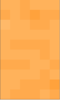
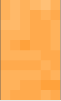
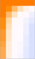
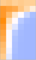
Depth $\longrightarrow$
Lower frequenciesHigher frequencies

Figure 1: We examine the complexity of the functions implemented by various MLP architectures. We find that much of their generalization capabilities can be understood independently from the optimization, training objective, scaling, or even data distribution. For example, ReLU and GELU networks (left) overwhelmingly represent low-frequency functions for any network depth or weight magnitude. Other activations lack this property.

The need for inductive biases.

The success of ML depends on using suitable inductive biases [45]. They specify how to generalize from a finite set of training examples to novel test cases. For example, linear models allow learning from few examples but generalize correctly only when the target function is itself linear. Large NNs are surprising in having large representational capacity [36] yet generalizing well across many tasks. In other words, among all learnable functions that fit the training data, those implemented by trained networks are often similar to the target function.

Explaining the success of neural networks.

Some successful architectures are tailored to specific domains e.g. CNNs for image recognition. But even the simplest MLP architectures (multi-layer perceptrons) often display remarkable generalization. Two explanations for this success prevail, although they are increasingly challenged.

• Implicit biases of gradient-based optimization. A large amount of work studies the preference of (stochastic) gradient descent or (S)GD for particular solutions [20, 51]. But conflicting results have also appeared. First, full-batch GD can be as effective as SGD [24, 38, 46, 69]. Second, Chiang et al. [9] showed that zeroth-order optimization can yield models with good generalization as frequently as GD. And third, Goldblum et al. [29] showed that language models with random weights already display a preference for low-complexity sequences. This “simplicity bias” was previously thought to emerge from training [65]. In short, gradient descent may help with generalization but it does not seem necessary.

• Good generalization as a fundamental property of all nonlinear architectures [33]. This vague conjecture does not account for the selection bias in the architectures and algorithms that researchers have converged on. For example, implicit neural representations (i.e. a network trained to represent a specific image or 3D shape) show that the success of NNs is not automatic and requires, in that case, activations very different from ReLUs.

The success of deep learning is thus not a product primarily of GD, nor is it universal to all architectures. This paper propose an explanation compatible with all above observations. It builds on the growing evidence that NNs benefit from their parametrization and the structure of their weight space [9, 29, 37, 64, 77, 79].

Contributions.

We present experiments supporting this three-part proposition (stated formally in Appendix C).

(1) NNs are biased to implement functions of a particular level of complexity (not necessarily low) determined by the architecture. (2) This preferred complexity is observable in networks with random weights from an uninformed prior. (3) Generalization is enabled by popular components like ReLUs setting this bias to a low complexity that often aligns with the target function.

We name it the Neural Redshift (NRS) by analogy to physical effects that bias the observations of a signal towards low frequencies. Here, the parameter space of NNs is biased towards functions of low frequency, one of the measures of complexity used in this work (see Figure 1).

The NRS differs from prior work on the spectral bias [57, 84] and simplicity bias [3, 65] which confound the effects of architectures and gradient descent. The spectral bias refers to the earlier learning of low-frequencies during training (see discussion in Section 6). The NRS only involves the parametrization of NNs and thus shows interesting properties independent from optimization [80], scaling [5], learning objectives [9], or even data distributions [52].

Concretely, we examine various architectures with random weights. We use three measures of complexity: (1) decompositions in Fourier series and (2) in bases of orthogonal polynomials (equating simplicity with low frequencies/order) and (3) compressibility as an approximation of the Kolmogorov complexity [15]. We study how they vary across architectures and how these properties at initialization correlate with the performance of trained networks.

Summary of findings.

• We verify the NRS with three notions of complexity that rely on frequencies in Fourier decompositions, order in polynomial decompositions, and compressibility of the input-output mapping (Section 3).

• We visualize the input-output mappings of 2D networks (Figure 3). They show intuitively the diversity of inductive biases across architectures that a scalar “complexity” cannot fully describe. Therefore, matching the complexity of an architecture with the target function is beneficial for generalization but hardly sufficient (Section 4.1).

• We show that the simplicity bias is not universal but depends on common components (ReLUs, residual connections, layer normalizations). ReLU networks also have the unique property of maintaining their simplicity bias for any depth and weight magnitudes. It suggests that the historical importance of ReLUs in the development of deep learning goes beyond the common narrative about vanishing gradients [42].

• We construct architectures where the NRS can be modulated (with alternative activations and weight magnitudes) or entirely avoided (parametrization in Fourier space, Section 3). It further demonstrates that the simplicity bias is not universal and can be controlled to learn complex functions (e.g. modulo arithmetic) or mitigate shortcut learning (Section 4.1).

• We show that the NRS is relevant to transformer sequence models. Random-weight transformers produce sequences of low complexity and this can also be modulated with the architecture. This suggests that transformers inherit inductive biases from their building blocks via mechanisms similar to those of simple models. (Section 5).

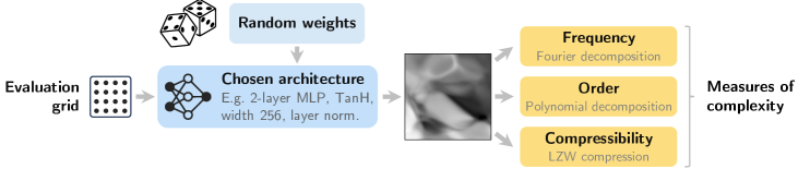
Figure 2: Our methodology to characterize the inductive biases of an architecture. We evaluate a network with random weights/biases on a grid of points. This yields a representation of the function implemented by the network, shown here as a grayscale image for a 2D input. We then characterize this function using three measures of complexity.

2 How to Measure Inductive Biases?

Our goal is to understand why NNs generalize when other models of similar capacity would often overfit. The immediate answer is simple: NNs have an inductive bias for functions with properties matching real-world data. Hence two subquestions.

1. What are these properties?
   We will show that three metrics are relevant: low frequency, low order, and compressibility. Hereafter, they are collectively referred to as “simplicity”.

2. What gives neural networks these properties?
   We will show that an overwhelming fraction of their parameter space corresponds to functions with such simplicity. While there exist solutions of arbitrary complexity, simple ones are found by default when navigating this space (especially with gradient-based methods).

Analyzing random networks.

Given an architecture to characterize, we propose to sample random weights and biases, then evaluate the network on a regular grid in its input space (see Figure 2). Let $f_{\boldsymbol{\theta}}({\boldsymbol{x}})$ represent the function implemented by a network of parameters ${\boldsymbol{\theta}}$ (weights and biases), evaluated on the input ${\boldsymbol{x}}\in\mathbb{R}^{d}$. The $f$ represents an architecture with a scalar output and no output activation, which could serve for any regression or classification task.

We sample weights and biases from an uninformed prior chosen as a uniform distribution. Biases are sampled from $\mathcal{U}(-1,1)$, and weights from the range proposed by Glorot and Bengio [28] commonly used for initialization i.e. $\mathcal{U}(-s,s)$ with $s=\alpha\,\sqrt{6\,/\,(\textrm{fan}_{\mathrm{in}}+\textrm{fan}_{\mathrm{out}})}$ where $\alpha$ is an extra factor ($1$ by default) to manipulate the weights’ magnitude in our experiments. These choices are not critical. Appendix E shows that other distributions (Gaussian, uniform-ball, long-tailed) lead to similar findings.

We then evaluate $f_{\boldsymbol{\theta}}(\cdot)$ on points ${\mathbf{X}}_{\mathrm{grid}}\!=\!\{{\boldsymbol{x}}_{1},\ldots,{\boldsymbol{x}}_{N}\}$ sampled regularly in the input space. We restrict ${\mathbf{X}}_{\mathrm{grid}}$ to the hypercube $[-1,+1]^{d}$ since the data used with NNs is commonly normalized. The evaluation of $f_{\boldsymbol{\theta}}(\cdot)$ on ${\mathbf{X}}_{\mathrm{grid}}$ yields a $d$-dimensional grid of scalars. In experiments of Section 3 where $d\!\!=\!\!2$, this is conveniently visualized as a 2D grayscale image to provide visual intuition about the function represented by the network. Next, we describe three quantifiable properties to extract from such representations.

Measures of complexity.

Applying the above procedure to various architectures with 2D inputs yields clearly diverse visual representations (see Figure 3). For quantitative comparisons, we propose three functions of the form $\operatorname{C}({\mathbf{X}}_{\mathrm{grid}},f)$ that estimate proxies of the complexity of $f$.

• Fourier frequency. A first natural choice is to use Fourier analysis as in classical signal and image processing. The “image” to analyze is the $d$-dimensional evaluation of $f$ on ${\mathbf{X}}_{\mathrm{grid}}$ mentioned above. We first compute a discrete Fourier transform that approximates $f$ with a weighted sum of sines of various frequencies. Formally, we have $f(x):=(2\pi)^{\nicefrac{{d}}{{2}}}\int\tilde{f}({\boldsymbol{k}})\,e^{i{\boldsymbol{k}}\cdot{\boldsymbol{x}}}d{\boldsymbol{k}}$ where $\tilde{f}({\boldsymbol{k}}):=\int f({\boldsymbol{x}})\,e^{-i{\boldsymbol{k}}\cdot{\boldsymbol{x}}}\mathbf{dx}$ is the Fourier transform. The discrete transform means that the frequency numbers ${\boldsymbol{k}}$ are regularly spaced, $\{0,1,2,\ldots,K\}$ with the maximum $K$ set according to the Nyquist–Shannon limit of ${\mathbf{X}}_{\mathrm{grid}}$. We use the intuition that complex functions are those with large high-frequency coefficients [57]. Therefore, we define our measure of complexity as the average of the coefficients weighted by their corresponding frequency i.e. $\operatorname{C}_{\text{Fourier}}(f)~{}=~{}\Sigma_{k=1}^{K}\tilde{f}({\boldsymbol{k}})\,k~{}~{}/~{}~{}\Sigma_{k=1}^{K}\tilde{f}({\boldsymbol{k}})$.

  For example, a smoothly varying function is likely to involve mostly low-frequency components, and therefore give a low value to $\operatorname{C}_{\text{Fourier}}$.

• Polynomial order. A minor variation of Fourier analysis uses decompositions in bases of polynomials. The procedure is nearly identical, except for the sine waves of increasing frequencies being replaced with fixed polynomials of increasing order (details in Appendix D). We obtain an approximation of $f$ as a weighted sum of such polynomials, and define our complexity measure $\operatorname{C}_{\text{Chebyshev}}$ exactly as above, i.e. the average of the coefficients weighted by their corresponding order. For example, the first two basis elements are a constant and a first-order polynomial, hence the decomposition of a linear $f$ will use large coefficients on these low-order elements and give a low complexity. We implemented this method with several canonical bases of orthogonal polynomials (Hermite, Legendre, and Chebyshev polynomials) and found the latter to be the most numerically stable.

• Compressibility has been proposed as an approximation of the Kolmogorov complexity [15, 29, 79]. We apply the classical Lempel-Ziv (LZ) compression on the sequence ${\mathbf{Y}}\!\!=\!\!\{f({\boldsymbol{x}}_{i})\!:{\boldsymbol{x}}_{i}\!\in\!{\mathbf{X}}\}$. We then use the size of the dictionary built by the algorithm as our measure of complexity $\operatorname{C}_{\text{LZ}}(f)$. A sequence with repeating patterns will require a small dictionary and give a low complexity.

3 Inductive Biases in Random Networks

We are now equipped to compare architectures. We will show that various components shift the inductive bias towards low or high complexity (see Table 1). In particular, ReLU activations will prove critical for a simplicity bias insensitive to depth and weight / activation magnitude.

Table 1: Components that bias NNs towards low/high complexity.

Lower complexity	No impact	Higher complexity
ReLU-like activations Small weights / activations Layer normalization Residual connections	Width Bias magnitudes	Other activations Large weights / activations Depth Multiplicative interactions

ReLU MLPs.

We start with a 1-hidden layer multi-layer perceptron (MLP) with ReLU activations. We will then examine variations of this architecture. Formally, each hidden layer applies a transformation on the input: ${\boldsymbol{x}}\!\leftarrow\!\phi({\boldsymbol{W}}{\boldsymbol{x}}+{\boldsymbol{b}})$ with weights ${\boldsymbol{W}}$, biases ${\boldsymbol{b}}$, and activation function $\phi(\cdot)$. MLPs are so simple that they are often thought as providing little or no inductive bias [5]. On the contrary, we observe in Figures 4 & 6 that MLPs have a very strong bias towards low-frequency, low-order, compressible functions. And this simplicity bias is remarkably unaffected by the magnitude of the weights, nor increased depth.

The variance in complexity across the random networks is essentially zero: virtually all of them have low complexity. This does not mean that they cannot represent complex functions, which would violate their universal approximation property [36]. Complex functions simply require precisely-adjusted weights and biases that are unlikely to be found by random sampling. These can still be found by gradient descent though, as we will see in Section 4.

ReLU-like activations

(GELU, Swish, SELU [16]) are also biased towards low complexity. Unlike ReLUs, close examination in Appendix F shows that increasing depth or weight magnitudes slightly increases the complexity.

Others activations

(TanH, Gaussian, sine) show completely different behaviour. Depth and weight magnitude cause a dramatic increase in complexity. Unsurprisingly, these activations are only used in special applications [58] with careful initializations [68]. Networks with these activations have no fixed preferred complexity independent of the weights’ or activations’ magnitudes. Mechanistically, the dependency on weight magnitudes is trivial to explain. Unlike with a ReLU, the output e.g. of a GELU is not equivariant to a rescaling of the weights and biases.

	ReLU	TanH
Weights $\sim$ $\mathcal{U}(-s,s)$
Weights $\sim$ $\mathcal{U}(-6s,6s)$

Figure 3: Comparison of functions implemented by random MLPs (2D input, 3 hidden layers). ReLU and TanH architectures are biased towards different functions despite their universal approximation capabilities. ReLU architectures have the unique property of maintaining their simplicity bias regardless of weight magnitude.

ReLU	GELU	Swish	SELU	Tanh	Gaussian	Sin	Unbiased

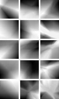
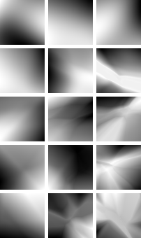
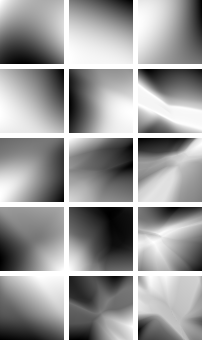
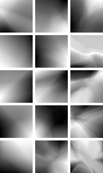
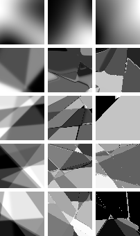
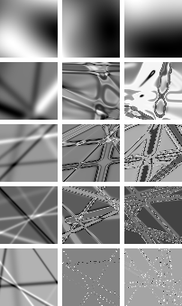
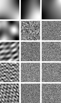
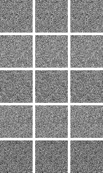
Figure 4: Heatmaps of the average Fourier complexity of functions implemented by random-weight networks. Each heatmap corresponds to an activation function and each cell (within a heatmap) corresponds to a depth (heatmap columns) and weight magnitude (heatmap rows). We also show grayscale images of functions implemented by networks of an architecture corresponding to every other heatmap cell.

	ReLU	GELU	Swish	SELU	TanH	Gaussian	Sin	Unbiased
Complexity (Fourier)

Figure 5: The complexity of random models (Y axis) generally increases with weights / activations magnitudes (X axis). The sensitivity is however very different across activation functions. This sensitivity also increases with multiplicative interactions (i.e. gating), decreases with residual connections, and is essentially absent with layer normalization.

Figure 6 shows close correlations between complexity measures, though they measure different proxies. Figure 3 shows that different activations make distinctive patterns not captured by the complexity measures. More work will be needed to characterize such fine-grained differences.

Width

has no impact on complexity, perhaps surprisingly. Additional neurons change the capacity of a model (what can be represented after training) but they do not affect its inductive biases. Indeed, the contribution of all neurons in a layer averages out to something invariant to their number.

Layer normalization

is a popular component in modern architectures, including transformers [55]. It shifts and rescales the internal representation to zero mean and unit variance [4]. We place layer normalizations before each activation such that each hidden layer now applies the transformation: ${\boldsymbol{x}}\!\leftarrow\!({\boldsymbol{W}}{\boldsymbol{x}}+{\boldsymbol{b}});~{}{\boldsymbol{x}}\!\leftarrow\!\phi(({\boldsymbol{x}}-\bar{{\boldsymbol{x}}})/\operatorname{std}({\boldsymbol{x}}))$ where $\bar{{\boldsymbol{x}}}$ and $\operatorname{std}({\boldsymbol{x}})$ denote the mean and standard deviation across channels. Layer normalization has the significant effect of removing variations in complexity with the weights’ magnitude for all activations (Figure 5). The weights can now vary (e.g. during training) without directly affecting the preferred complexity of the architecture. Layer normalizations also usually apply a learnable offset ($0$ by default) and scaling ($1$ by default) post-normalization. Given the above observations, when paired with an activation with some slight sensitivity to weight magnitude (e.g. GELUs, see Appendix F), this scaling can now be interpreted as a learnable shift in complexity, modulated by a single scalar (rather than the whole weight matrix without the normalization).

Residual connections

[31]. We add these such that each non-linearity is now described with: ${\boldsymbol{x}}\!\leftarrow\!(x+\phi({\boldsymbol{x}}))$. This has the dramatic effect of forcing the preferred complexity to some of the lowest levels for all activations regardless of depth. This can be explained by the fact that residual connections essentially bypass the stacking of non-linearities that causes the increased complexity with increased depth.

Multiplicative interactions

refer to multiplications of internal representations with one another [39] as in attention layers, highway networks, dynamic convolutions, etc. We place them in our MLPs as gating operations, such that each hidden layer corresponds to: ${\boldsymbol{x}}\!\leftarrow\!\big{(}\phi(W{\boldsymbol{x}}+b)~{}\odot~{}\sigma(W^{\prime}{\boldsymbol{x}}+b^{\prime})\big{)}$ where $\sigma(\cdot)$ is the logistic function. This creates a clear increase in complexity dependent on depth and weight magnitude, even for ReLU activations. This agrees with prior work showing that multiplicative interactions in polynomial networks [10] facilitate learning high frequencies.

Unbiased model.

As a counter-example to models showing some preferred complexity, we construct an architecture with no bias by design in the complexity measured with Fourier frequencies. This special architecture implements an inverse Fourier transform, parametrized directly with the coefficients and phase shifts of the Fourier components (details in Appendix D). The inverse Fourier transform is a weighted sum of sine waves, so this architecture can be implemented as a one-layer MLP with sine activations and fixed input weights representing each one Fourier component. These fixed weights prior to sine activations thus enforce a uniform prior over frequencies.

This architecture behaves very differently from standard MLPs (Figure 4). With random weights, its Fourier spectrum is uniform, which gives a high complexity for any weight magnitude (depth is fixed). Functions implemented by this architecture look like white noise. Even though this architecture can be trained by gradient descent like any MLP, we show in Appendix E that it is practically useless because of its lack of any complexity bias.

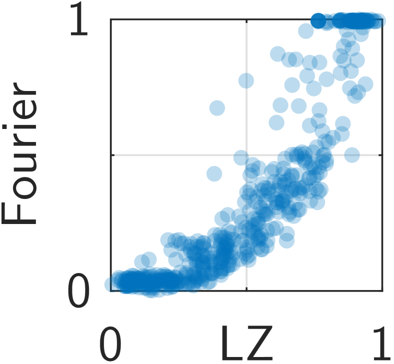
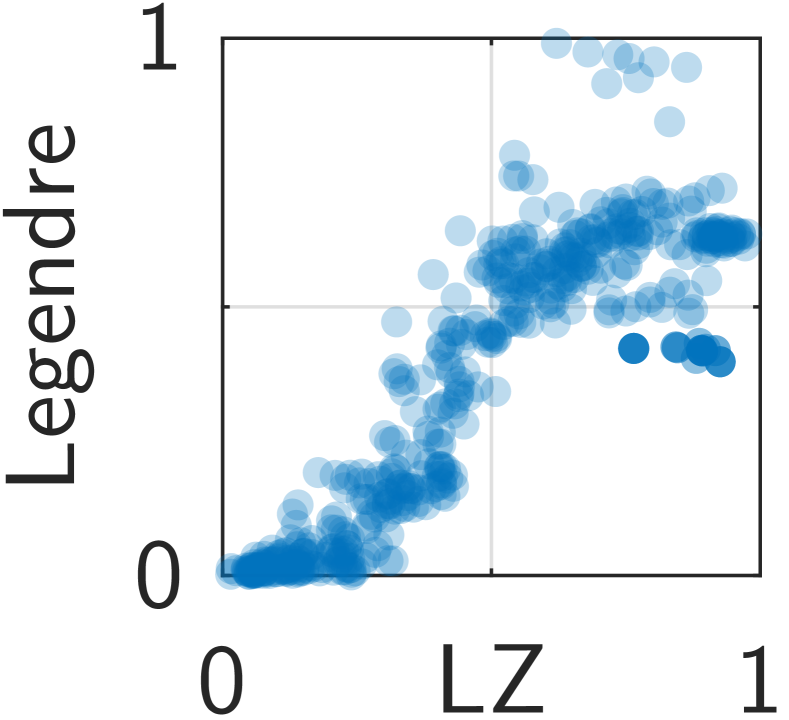
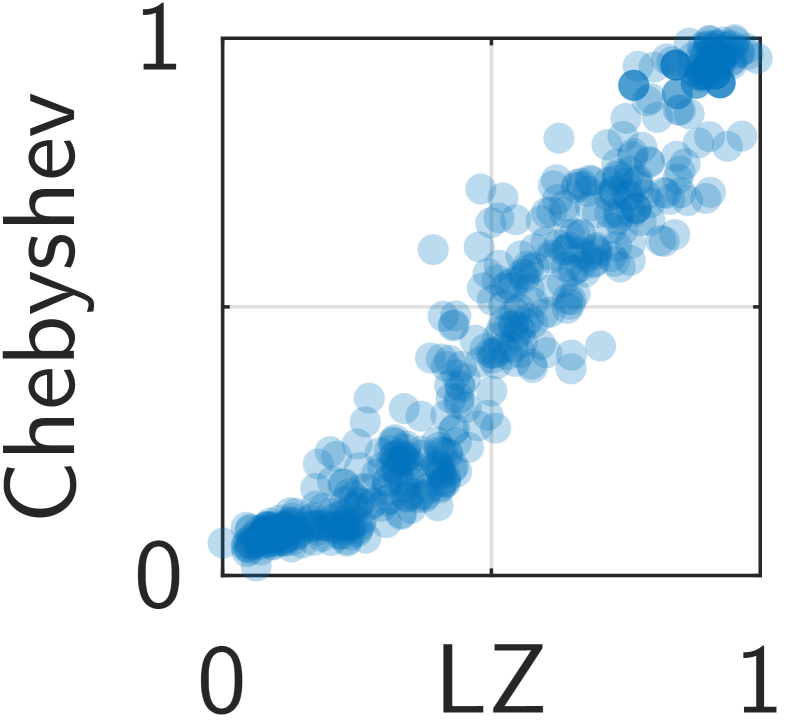
Figure 6: Our various complexity measures are closely correlated despite measuring each a different proxy i.e. frequency (Fourier), polynomial order (Legendre, Chebyshev), or compressibility (LZ).

Importance of ReLU activations
The fact that a strong simplicity bias depends on ReLU activations suggests that their historical importance in the development of deep learning goes beyond the common narrative about vanishing gradients [42]. The same may apply to residual connections and layer normalization since they alsox contribute strongly to the simplicity bias. This contrasts with the current literature that mostly invokes their numerical properties [6, 82, 83].

4 Inductive Biases in Trained Models

We now examine how the inductive biases of an architecture impact a model trained by standard gradient descent. We will show that there is a strong correlation between the complexity at initialization (i.e. with random weights as examined in the previous section) and in the trained model. We will also see that unusual architectures with a bias towards high complexity can improve generalization on tasks where the standard “simplicity bias” is suboptimal.

4.1 Learning Complex Functions

The NRS proposes that good generalization requires a good match between the complexity preferred by the architecture and the target function. We verify this claim by demonstrating improved generalization on complex tasks with architectures biased towards higher complexity. This is also a proof of concept of the potential utility of controlling inductive biases.

Experimental setup.

We consider a simple binary classification task involving modulo arithmetic. Such tasks like the parity function [66] are known to be challenging for standard architectures because they contain high-frequency patterns. The input to our task is a vector of integers ${\boldsymbol{x}}\!\in\![0,N\!-\!1]^{d}$. The correct labels are ${\mathbb{1}}(\Sigma x_{i}\leq(M/2)\operatorname{mod}M)$. We consider three versions with $N\!=\!16$ and $M\!=\!\{10,7,4\}$ that correspond to increasingly higher frequencies in the target function (see Figure 7 and Appendix D for details).

Results.

We see in Figure 7 that a ReLU MLP only solves the low-frequency version of the task. Even though this model can be trained to perfect training accuracy on the higher-frequency versions, it then fails to generalize because of its simplicity bias. We then train MLPs with other activations (TanH, Gaussian, sine) whose preferred complexity is sensitive to the activations’ magnitude. We also introduce a constant multiplicative prefactor before each activation function to modulate this bias without changing the weights’ magnitude, which could introduce optimization side effects. Some of these models succeed in learning all versions of the task when the prefactor is correctly tuned. For higher-frequency versions, the prefactor needs to be larger to shift the bias towards higher complexity. In Figure 7, we fit a quadratic approximation to the accuracy of Gaussian-activated models. The peak then clearly shifts to the right on the complex tasks. This agrees with the NRS proposition that complexity at initialization relates to properties of the trained model.

Let us also note that not all activations succeed, even with a tuned prefactor. This shows that matching the complexity of the architecture and of the target function is beneficial but not sufficient for good generalization. The inductive biases of an architecture are clearly not fully captured by any of our measures of complexity.

	Target function (3 versions of “modulo addition”)
	Low freq.	Med. freq.	High freq.
Test accuracy
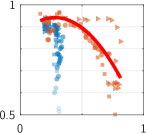
	Complexity (LZ) at initialization
	(modulated by choices of activation and prefactor value)

Figure 7: Results training networks on three tasks of increasing complexity. Each point represents a different architecture. ReLU-like activations are biased towards low complexity and fail to generalize on complex tasks. With other activations, the complexity bias depends on the activation magnitudes, which we can control with a multiplicative prefactor. This enables generalization on complex tasks by shifting the bias to higher complexity. Indeed, the optimum prefactor (peak of the quadratic fit) shifts to the right on each task of increasing complexity.

	Low frequency	Medium frequency	High frequency
Test accuracy

Figure 8: Detail of Figure 7 for Gaussian activations. The peak accuracy shifts to the right on tasks of increasing complexity. This corresponds to a larger prefactor that shifts the bias towards higher complexity. Each point represents one random seed.

Reinterpretation of existing work
Loss landscapes Are All You Need [9]
Chiang et al. showed that networks with random weights, as long as they fit the training data with low training loss, are good solutions that generalize to the test data. We find “loss landscapes” slightly misleading because the key is in the parametrization of the network (and by extension of this landscape) and not in the loss function. Their results can be replicated by replacing the cross-entropy loss with an MSE loss, but not by replacing their MLP with our “unbiased learner” architecture. The sampled solutions are good, not only because of their low training loss, but because they are found by uniformly sampling the weight space. Bad low-loss solutions also exist, but they are unlikely to be found by random sampling. Because of the NRS, all random-weight networks implement simple functions, which generalize as long as they fit the training data. An alternative title could be “Uniformly Sampling the Weight Space Is All You Need”.

4.2 Impact on Shortcut Learning

Shortcut learning refers to situations where the simplicity bias causes a model to rely on simple spurious features rather than learning the more-complex target function [65].

Experimental setup.

We consider a regression task similar to Colored-MNIST. Inputs are images of handwritten digits juxtaposed with a uniform band of colored pixels that simulate spurious features. The labels in the training data are values in $[0,1]$ proportional to the digit value as well as to the color intensity. Therefore, a model can attain high training accuracy by relying either on the simple linear relation with the color, or the more complex recognition of the digits (the target task). To measure the reliance of a model on color or digit, we use two test sets where either the color or digit is correlated with the label while the other is randomized. See Appendix D for details.

Results.

We train 2-layer MLPs with different activation functions. We also use a multiplicative prefactor, i.e. a constant $\alpha\!\in\!\mathrm{R}^{+}$ placed before each activation function such that each non-linear layer performs the following: ${\boldsymbol{x}}\!\leftarrow\!\phi\big{(}\alpha(W{\boldsymbol{x}}+b)\big{)}$. The prefactor mimics a rescaling of the weights and biases with no optimization side effects.

We see in Figure 9 that the LZ complexity at initialization increases with prefactor values for TanH, Gaussian, and sine activations. Most interestingly, the accuracy on the digit and color also varies with the prefactor. The color is learned more easily with small prefactors (corresponding to a low complexity at initialization) while the digit is learned more easily at an intermediate value (corresponding to medium complexity at initialization). The best performance on the digit is reached at a sweet spot that we explain as the hypothesized “best match” between the complexity of the target function, and that preferred by the architecture. With larger prefactors, i.e. beyond this sweet spot, the accuracy on the digit decreases, and even more so with sine activations for which the complexity also increases more rapidly, further supporting the proposed explanation.

	TanH	Gaussian	Sine
Test accuracy      Complexity at init. (LZ)

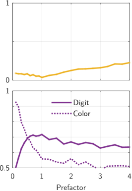
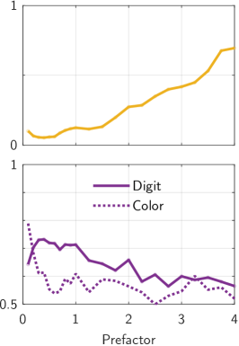
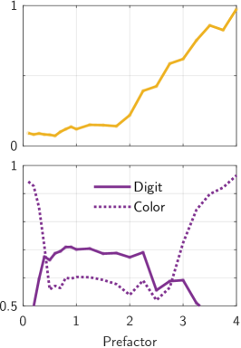
Figure 9: Experiments on Colored-MNIST show a clear correlation between complexity at initialization (top) and test accuracy (bottom). Models with a bias for low complexity rely on the color i.e. the simpler feature. The accuracy on the digit peaks at a sweet spot where the models’ preferred complexity matches the digits’.

Reinterpretation of existing work
How You Start Matters for Generalization [59]
Ramasinghe et al. examine implicit neural representations (i.e. a network trained to represent one image). They observe that models showing high frequencies at initialization also learn high frequencies better. They conclude that complexity at initialization causally influences the solution. But our results suggest instead that these are two effects of a common cause: the architecture is biased towards a certain complexity, which influences both the untrained model and the solutions found by gradient descent. There exist configurations of weights that correspond to complex functions, but they are unlikely to be found in either case. Appendix E.3 shows that initializing GD from such a solution with an architecture biased toward simplicity does not yield complex solutions, thus disproving the causal relation.

5 Transformers are Biased Towards
Compressible Sequences

We now show that the inductive biases observed with MLPs are relevant to transformer sequence models. The experiments below confirm the bias of a transformer for generating simple, compressible sequences [29] which could then explain the tendency of language models to repeat themselves [21, 34]. The experiments also suggest that transformers inherit this inductive bias from the same components as those explaining the simplicity bias in MLPs.

Experimental setup.

We sample sequences from an untrained GPT-2 [55]. For each sequence, we sample random weights from their default initial distribution, then prompt the model with one random token (all of them being equivalent since the model is untrained), then generate a sequence of 100 tokens by greedy maximum-likelihood decoding. We evaluate the complexity of each sequence with the LZ measure (Section • ‣ 2) and report the average over 1,000 sequences. We evaluate variations of the architecture: replacing activation functions in MLP blocks (GELUs by default), varying the depth ($12$ transformer blocks by default), and varying the activations’ magnitude by modifying the scaling factor in layer normalizations ($1$ by default).

Results.

We first observe in Figure 10 that the default architecture is biased towards relatively simple sequences. This observation, already reported by Goldblum et al. [29], is non-trivial since a random model could as well generate completely random sequences. Changing the activation function from the default GELUs has a large effect. The complexity increases with SELU, TanH, sine, and decreases with ReLU. It is initially low with Gaussian activations, but climbs higher than most others with larger activation magnitudes. This is consistent with observations made on MLPs, where ReLU induced the strongest bias for simplicity, and TanH, Gaussian, sine for complexity. Variations of activations’ magnitude (via scaling in layer normalizations) has the same monotonic effect on complexity as observed in MLPs. However, we lack an explanation for the “shoulders” in the curves of SELU, Tanh, and sine. It may relate to them being the activations that output negative values most. Varying depth also has the expected effect of magnifying the differences across activations and scales.

Complexity (LZ)
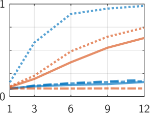
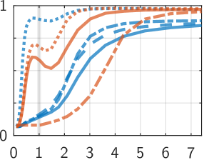
	Depth (num. of transformer	Scaling in layer
	blocks, scaling=1)	normalization (depth=12)

Figure 10: Average complexity (LZ) of sequences generated by an untrained GPT-2. Variations of the architecture correspond to variations in complexity comparable to MLPs. This suggests that transformers inherit a bias for simple sequences from their building blocks via mechanisms similar to those in simple models.

Take-away.

These results suggest that the bias for simple sequences of transformers originates from their building blocks via similar mechanisms to those causing the simplicity bias in other predictive models. The building blocks of transformers also seem to balance a shift towards higher complexity (attention, multiplicative interactions) and lower complexity (GELUs, layer normalizations, residual connections).

6 Related Work

Much effort has gone into explaining the success of deep learning through the inductive biases of SGD [48] and structured architectures [11, 90]. This work rather focuses on implicit inductive biases from unstructured architectures.

The simplicity bias is the tendency of NNs to fit data with simple functions [3, 25, 53, 75]. The spectral bias suggests that NNs prioritize learning low-frequency components of the target function [57, 84]. These studies confound architectures and optimization. And most explanations invoke implicit regularization of gradient descent [70, 85] and are specific to ReLU networks [35, 38, 88]. In contrast, we show that some form of spectral bias exists in common architectures independently of gradient descent.

A related line of study showed that Boolean MLPs are biased towards low-entropy functions [12, 44]. Work closer to ours [12, 44, 79] examines the simplicity bias of networks with random weights. These works are limited to MLPs with binary inputs or outputs [12, 44], ReLU activations, and simplicity measured as compressibility. In contrast, our work examines multiple measures of simplicity and a wider set of architectures. In work concurrent to ours, Abbe et al. [1] used Walsh decompositions (analogous to Fourier series for binary functions) to characterize the simplicity of learned binary classification networks. Their discussion is specific to classification and highly complementary to ours.

Our work also provides a new lens to explain why choices of activation functions are critical [16, 60, 67]. See Appendix A for an extended literature review.

7 Conclusions

We examined inductive biases that NNs possess independently of their optimization. We found that the parameter space of popular architectures corresponds overwhelmingly to functions with three quantifiable properties: low frequency, low order, and compressibility. They correspond to the simplicity bias previously observed in trained models which we now explain without involving (S)GD. We also showed that the simplicity bias is not universal to all architectures. It results from ReLUs, residual connections, layer normalization, etc. The popularity of these components likely reflects the collective search for architectures that perform well on real-world data. In short, the effectiveness of NNs is not an intrinsic property but the result of the adequacy between key choices (e.g. ReLUs) and properties of real-world data (prevalence of low-complexity patterns).

Limitations and open questions.

• Our analysis used mostly small models and data to enable visualizations (2D function maps) and computations (Fourier decompositions). We showed the relevance of our findings to large transformers, but the study could be extended to other large architectures and tasks.

• Our analysis relies on empirical simulations. It could be carried out analytically to provide theoretical insights.

• Our results do not invalidate prior work on implicit biases of (S)GD. Future work should clarify the interplay of different sources of inductive biases. Even if most of the parameter space corresponds to simple functions, GD can navigate to complex ones. Are they isolated points in parameter space, islands, or connected regions? This relates to mode connectivity, lottery tickets [19], and the hypothesis that good flat minima occupy a large volume [37].

• We proposed three quantifiable facets of inductive biases. Much is missed about the “shape” of functions preferred by different activations (Figure 3). An extension could discover other reasons for the success of NNs and fundamental properties shared across real-world datasets.

• An application of our findings is in the control of inductive biases to nudge the behaviour of trained networks [87]. For example by manipulating the parametrization of NNs on which (S)GD is performed.

Supplementary Material

Appendix A Additional Related Work

A vast literature examines the success of deep learning using inductive biases of optimization methods (e.g. SGD [48]) and architectures (e.g. CNNs [11], transformers [90]). This paper instead examines implicit inductive biases in unstructured architectures.

Parametrization of NNs.

It is challenging to understand the structure and “effective dimensionality” of the weight space of NNs because multiple weight configurations and their permutations correspond to the same function [17, 71, 89]. A recent study quantified the information needed to identify a model with good generalization [8]. However, the estimated values are astronomical (meaning that no dataset would ever be large enough to learn the target function). Our work reconciles these results with the reality (the fact that deep learning does work in practice) by showing that the overlap of the set of good generalizing functions with uniform samples in weight space [8, Fig. 1] is much denser than its overlap with truly random functions. In other words, random sampling in weight space generally yields functions likely to generalize. Much less information is needed to pick one solution among those than estimated in [8].

Some think that “stronger inductive biases come at the cost of decreasing the universality of a model” [13]. This is a misunderstanding of the role of inductive biases: they are fundamentally necessary for machine learning and they do not imply a restriction on the set of learnable functions. We show in particular that MLPs have strong inductive biases yet remain universal.

The simplicity bias

refers to the observed tendency of NNs to fit their training data with simple functions. It is desirable when it prevents overparametrized networks from overfitting the training data [3, 53]. But it is a curse when it causes shortcut learning [25, 75]. Most papers on this topic are about trained networks, hence they confound the inductive biases of the architectures and of the optimization. Most explanations of the simplicity bias involve loss functions [52] and gradient descent [2, 32, 41, 73].

Work closer to ours [12, 44, 79] examines the simplicity bias of networks with random weights. These studies are limited to MLPs with binary inputs/outputs, ReLU activations, and/or simplicity measured as compressibility. In contrast, we examine more architectures and other measures of complexity. Earlier works with random-weight networks include [56, 27, 40, 43, 23, 54, 63, 50].

Goldblum et al. [29] proposed that NNs are effective because they combine a simplicity bias with a flexible hypothesis space. Thus they can represent complex functions and benefit from large datasets. Our results also support this argument.

The spectral bias

[57] or frequency principle [84] is a particular form of the simplicity bias. It refers to the observation that NNs learn low-frequency components of the target function earlier during training. Works on this topic are specific to gradient descent [70, 85]. and often to ReLU networks [35, 38, 88]. Our work is about properties of architectures independent of the training.

Work closer to ours [86] has noted that the spectral bias exists with ReLUs but not with sigmoidal activations, and that it depends on weight magnitudes and depth (all of which we also observe in our experiments). Their analysis uses the neural tangent kernel (NTK) whereas we use a Fourier decomposition of the learned function, which is arguably more direct and intuitive. We also examine other notions of complexity, and other architectures.

In work concurrent to ours, Abbe et al. [1] used Walsh decompositions (a variant of Fourier analysis suited to binary functions) to characterize learned binary classification networks. They also propose that typical NNs preferably fit low-degree basis functions to the training data and this explains their generalization capabilities. Their discussion, which focuses on classification tasks, is highly complementary to ours.

The “deep image prior” [78] is an image processing method that exploit the inductive biases of an untrained network. However it specifically relies on convolutional (U-Net) architectures, whose inductive biases have little to do with those studied in this paper.

Measures of complexity.

Quantifying complexity is an open problem in the fundamental sciences. Algorithmic information theory (AIT) and Kolmogorov complexity are one formalization of this problem. Kolmogorov complexity has been proposed as an explicit regularizer to train NNs by Schmidhuber [62]. Dingle et al. [15] used AIT to explain the prevalence of simplicity in the real-world with examples in biology and finance. Building on this work, Valle-Perez et al. [79] showed that binary ReLU networks with random weights have a similar bias for simplicity. Our work extends this line of inquiry to continuous data, to other architectures, and to other notions of complexity.

Other measures of complexity for to machine learning models include four related notions: sensitivity, Lipschitz constant, norms of input gradients, and Dirichlet energy [14]. Hahn et al. [30] adapted “sensitivity” to the discrete nature of language data to measure the complexity of language classification tasks and of models.

Simplicity bias in transformers.

Zhou et al. [90] explain generalization of transformer models on toy reasoning tasks using a transformer-specific measure of complexity. They propose that the function learned by a transformer corresponds to the shortest program (in a custom programming language) that could generate the training data. Bhattamishra et al. [7] showed that transformers are more biased for simplicity than LSTMs.

Controlling inductive biases.

Recent work has investigated how to explicitly tweak the inductive biases of NNs through learning objectives [75, 76] and architectures [10, 74]. Our results confirms that the choice of activation function is critical [16]. Most studies on activation functions focus on individual neurons [63] or compare the generalization properties of entire networks [49]. Francazi et al. [18] showed that some activations cause a model at initialization to have non-uniform preference over classes. Simon et al. [67] showed that the behaviour of a deep MLP can be mimicked by a single-layer MLP with a specifically-crafted activation function.

Implicit neural representations

(INRs) are an application of NNs with a need to control their spectral bias. An INR is a regression network trained to represent e.g. one specific image by mapping image coordinates to pixel intensities (they are also known as neural fields or coordinate MLPs). To represent sharp image details, a network must represent a high-frequency function, which is at odds with the low-frequency bias of typical architectures. It has been found that replacing ReLUs with periodic functions [81, Sect. 5], Gaussians [58], or wavelets [61] can shift the spectral bias towards higher frequencies [60]. Interestingly, such architectures (Fourier Neural Networks) were investigated as early as 1988 [22]. Our work shows that several findings about INRs are also relevant to general learning tasks.

Appendix B Why study networks with random weights?

A motivation can be found in prior work that argued for interpreting the inductive biases of an architecture as a prior over functions that plays in the training of the model by gradient descent.

Valle-Perez et al. [79] and Mingard et al. [44] argued that the probability of sampling certain functions upon random sampling in parameter space could be treated as a prior over functions for Bayesian inference. They then presented preliminary empirical evidence that training with SGD does approximate Bayesian inference, such that the probability of landing on particular solutions is proportional to their prior probability when sampling random parameters.

Appendix C Formal Statement of the NRS

We denote with

• $F$: the target function we want to learn;

• $f_{\boldsymbol{\theta}}$: a chosen neural architecture with parameters ${\boldsymbol{\theta}}$;

• $f^{\star}\!:=\!f_{{\boldsymbol{\theta}}^{\star}}$: a trained network with ${\boldsymbol{\theta}}^{\star}$ optimized s.t. $f^{\star}$ approximates $F$;

• $\bar{f}\!:=\!f_{\bar{{\boldsymbol{\theta}}}},~{}~{}\bar{{\boldsymbol{\theta}}}\!\!\sim\!\!p_{\text{prior}}({\boldsymbol{\theta}})$: an untrained random-weight network with parameters drawn from an uninformed prior, such as the uniform distribution used to initialize the network prior to gradient descent.

• $\operatorname{C}(f)$: a scalar estimate the of complexity of the function $f$ as proposed in Section 2;

• $\operatorname{perf}(f)$: a scalar measure of generalization performance i.e. how well $f$ approximates $F$, for example the accuracy on a held-out test set.

The Neural Redshift (NRS) makes three propositions.

1. NNs are biased to implement functions of a particular level of complexity determined by the architecture.

2. This preferred complexity is observable in networks with random weights from an uninformed prior.

   Formally, $\forall$ architecture $f$, distribution $p_{\text{prior}}({\boldsymbol{\theta}})$,
   $\exists$ preferred complexity $c\in\mathbb{R}$ s.t.

   $$\operatorname{C}(\bar{f}) =c~{}~{}~{}~{}~{}~{}\textrm{with very high probability, and}$$

   $$\operatorname{C}(f^{\star}) =g(c)~{}\textrm{with}~{}~{}g:\mathbb{R}\rightarrow\mathbb{R}~{}~{}\textrm{a monotonic function.}$$

   This means that the choice of architecture shifts the complexity of the learned function up or down similarly as it does an untrained model’s. The precise shift is usually not predictable because $g(\cdot)$ is unknown.

3. Generalization occurs when the preferred complexity of the architecture matches the target function’s.

   Formally, given two architectures $f_{1}$, $f_{2}$ with preferred complexities $c_{1}$, $c_{2}$, the one with a complexity closer to the target function’s achieves better generalization:

   $$|\operatorname{C}(F)-g(c_{1})|\,~{} <~{}\,|\operatorname{C}(F)-g(c_{2})|$$

   $$\Longrightarrow~{}~{}\operatorname{perf}(f_{1}^{\star})\,~{} >~{}\,\operatorname{perf}(f_{2}^{\star})\,.$$

   For example, ReLUs are popular because their low-complexity bias often aligns with the target function.

Appendix D Technical Details

Activation functions.

See Figure 11 for a summary of the activations used in our experiments and [16] for a survey.

$\operatorname{max}(0,x)$	$x.P_{\mathrm{Gaussian}}(X\!\leq\!x)$	$x.\sigma(x)$	$\lambda\begin{cases}\alpha\,(e^{x}\!-\!1),&\!\!\!x\!\leq\!0\\ x,&\!\!\!x\!>\!0\end{cases}$	$\operatorname{tanh}(x)$	$e^{(-0.5\,x^{2})}$	$\operatorname{sin}(x)$

Figure 11: Activation functions used in our experiments.

Discrete network evaluation.

For a given network that implements the function $f({\boldsymbol{x}})$ of input ${\boldsymbol{x}}\in\mathbb{R}^{d}$, we obtain obtain a discrete representation as follows. We define a sequence of points ${\mathbf{X}}_{\mathrm{grid}}\!=\!\{{\boldsymbol{x}}_{i}\}_{i=1}^{m^{d}}$ corresponding to a regular grid on the $d$-dimensional hypercube $[-1,1]^{d}$, with $m$ values in each dimension ($m\!\mathrel{\mkern 0.2mu\mathchoice{\scalebox{0.5}[1.0]{$\displaystyle=$}}{\scalebox{0.5}[1.0]{$\textstyle=$}}{\scalebox{0.5}[1.0]{$\scriptstyle=$}}{\scalebox{0.5}[1.0]{$\scriptscriptstyle=$}}\mkern 0.2mu}\!64$ in our experiments) hence $m^{d}$ points in total. We evaluate the network on every point. This gives the sequence of scalars ${\mathbf{Y}}_{f}\!=\!\{f({\boldsymbol{x}}_{i})\!:{\boldsymbol{x}}_{i}\!\in\!{\mathbf{X}}_{\mathrm{grid}}\}$.

Visualizations as grayscale images.

For a network $f$ with 2D inputs ($d\!\mathrel{\mkern 0.2mu\mathchoice{\scalebox{0.5}[1.0]{$\displaystyle=$}}{\scalebox{0.5}[1.0]{$\textstyle=$}}{\scalebox{0.5}[1.0]{$\scriptstyle=$}}{\scalebox{0.5}[1.0]{$\scriptscriptstyle=$}}\mkern 0.2mu}\!2$) we produce a visualization as a grayscale image as follows. The values in ${\mathbf{Y}}_{f}$ are simply scaled and shifted to fill the range from black ($0$) to white ($1$) as:

$\tilde{{\mathbf{Y}}}=({\mathbf{Y}}\!-\!\operatorname{min}({\mathbf{Y}}))\,/\,(\operatorname{max}({\mathbf{Y}})\!-\!\operatorname{min}({\mathbf{Y}}))$.

We then reshape $\tilde{{\mathbf{Y}}}$ into an $m\times m$ square image.

Measures of complexity.

We use our measures of complexity based on Fourier and polynomial decompositions only with $d\!\mathrel{\mkern 0.2mu\mathchoice{\scalebox{0.5}[1.0]{$\displaystyle=$}}{\scalebox{0.5}[1.0]{$\textstyle=$}}{\scalebox{0.5}[1.0]{$\scriptstyle=$}}{\scalebox{0.5}[1.0]{$\scriptscriptstyle=$}}\mkern 0.2mu}\!2$ because of the computational expense. These methods first require an evaluation of the network on a discrete grid as described above (${\mathbf{Y}}_{f}$) whose size grows exponentially in the number of dimensions $d$.

Xu et al. [84] proposed two approximations for Fourier analysis in higher dimensions. They were not used in our experiments but could be valuable for extensions of our work to higher-dimensional settings.

Fourier decomposition.

To compute the measure of complexity $\operatorname{C}_{\text{Fourier}}(f)$, we first precompute values of $f$ on a discrete grid ${\mathbf{X}}_{\mathrm{grid}}$, yielding ${\mathbf{Y}}_{f}$ as describe above. We then perform a standard discrete Fourier decomposition with these precomputed values. We get:

$\tilde{f}({\boldsymbol{k}})=\Sigma_{{\boldsymbol{x}}\in{\mathbf{X}}_{\mathrm{grid}}}\,\omega^{{\boldsymbol{x}}^{\intercal}{\boldsymbol{k}}}\,f({\boldsymbol{x}})$

where $\omega\!=\!e^{-2\pi i/m}$ and ${\boldsymbol{k}}\in\mathbb{Z}^{d}$ are discrete frequency numbers. Per the Nyquist-Shannon theorem, with an evaluation of $f$ on a grid of $m$ values in each dimension, we can reliably measure the energy for frequency numbers up to $m/2$ in each dimension i.e. for ${\boldsymbol{k}}\in{\mathbf{K}}\!=\![0,$ . . .$,m/2]^{d}$.

The value $\tilde{f}({\boldsymbol{k}})$ is a complex number that captures both the magnitude and phase of the ${\boldsymbol{k}}$th Fourier component. We do not care about the phase, hence our measure of complexity only uses the real magnitude $|\tilde{f}({\boldsymbol{k}})|$ of each Fourier component ${\boldsymbol{k}}$. We then seek to summarize the distribution of these magnitudes across frequencies into a single value. We define the measure of complexity:

$\operatorname{C}_{\text{Fourier}}(f)~{}=~{}\Sigma_{{\boldsymbol{k}}\in{\mathbf{K}}}\,|\tilde{f}({\boldsymbol{k}})|\,.\,||{\boldsymbol{k}}||_{2}\;~{}/\;~{}\Sigma_{{\boldsymbol{k}}\in{\mathbf{K}}}\,|\tilde{f}({\boldsymbol{k}})|$.

This is the average of magnitudes, weighted each by the corresponding frequency, disregarding orientation (e.g. horizontal and vertical patterns in a 2D visualization of the function are treated similarly), and normalized such that magnitudes sum to $1$.

See [57] for a technical discussion justifying Fourier analysis on non-periodic bounded functions.

Limitations of a scalar measure of complexity.

The above definition is necessarily imperfect at summarizing the distributions of magnitudes across frequencies. For example, an $f$ containing both low and high-frequencies could receive the same value as one containing only medium frequencies. In practice however, we use this complexity measure on random networks, and we verified empirically that the distributions of magnitudes are always unimodal. This summary statistic is therefore a reasonable choice to compare distributions.

Polynomial decomposition.

As an alternative to Fourier analysis, we use decomposition in polynomial series. It uses a predefined set of polynomials $P_{n}(x)$, $n=[0,$ . . .$,N]$ to approximate a function $f(x)$ on the interval $x\in[-1,1]$ as $f(x)\!\approx\!\Sigma_{c=0}^{N}\,c_{n}P_{n}(x)$. The coefficients are calculated as $c_{n}\!=\!0.5\,(2n+1)\,\int_{-1}^{+1}f(x)\,P_{n}(x)\,dx$. These definitions readily extends to higher dimensions.

In a Fourier decomposition, the coefficients indicate the amount the various frequency components in $f$. Here, each coefficient $c_{n}$ indicates the amount of a component of a certain order. In 2 dimensions ($d\!\mathrel{\mkern 0.2mu\mathchoice{\scalebox{0.5}[1.0]{$\displaystyle=$}}{\scalebox{0.5}[1.0]{$\textstyle=$}}{\scalebox{0.5}[1.0]{$\scriptstyle=$}}{\scalebox{0.5}[1.0]{$\scriptscriptstyle=$}}\mkern 0.2mu}\!2$), we have $N^{2}$ coefficients $c_{00},c_{01},$ . . .$,c_{NN}$. We define our measure of complexity:

$\operatorname{C}_{\text{Chebyshev}}(f)~{}=~{}\frac{\Sigma_{n_{1},n_{2}\mathrel{\mkern 0.2mu\mathchoice{\scalebox{0.5}[1.0]{$\displaystyle=$}}{\scalebox{0.5}[1.0]{$\textstyle=$}}{\scalebox{0.5}[1.0]{$\scriptstyle=$}}{\scalebox{0.5}[1.0]{$\scriptscriptstyle=$}}\mkern 0.2mu}0}^{N}\,|c_{n_{1}n_{2}}|\,.\,||\,[n_{1},n_{2}]\,||_{2}}{\Sigma_{n1,n2\mathrel{\mkern 0.2mu\mathchoice{\scalebox{0.5}[1.0]{$\displaystyle=$}}{\scalebox{0.5}[1.0]{$\textstyle=$}}{\scalebox{0.5}[1.0]{$\scriptstyle=$}}{\scalebox{0.5}[1.0]{$\scriptscriptstyle=$}}\mkern 0.2mu}0}^{N}\,|c_{n1,n2}|}$.

This definition is nearly identical to the Fourier one.

In practice, we experimented with Hermite, Legendre, and Chebyshev bases of polynomials. We found the latter to be more numerically stable. To compute the coefficients, we use trapezoidal numerical integration and the same sampling of $f$ on ${\mathbf{X}}_{\mathrm{grid}}$ as described above, and a maximum order $N\!\mathrel{\mkern 0.2mu\mathchoice{\scalebox{0.5}[1.0]{$\displaystyle=$}}{\scalebox{0.5}[1.0]{$\textstyle=$}}{\scalebox{0.5}[1.0]{$\scriptstyle=$}}{\scalebox{0.5}[1.0]{$\scriptscriptstyle=$}}\mkern 0.2mu}\!100$. To make the evaluation of the integrals more numerically stable (especially with Legendre polynomials), we omit a border near the edges of the domain $[-1,1]^{d}$. With a $64\times 64$ grid, we omit 3 values on every side.

LZ Complexity.

We use the compression-based measure of complexity described in [15, 79] as an approximation of the Kolmogorov complexity. We first evaluate $f$ on a grid to get ${\mathbf{Y}}_{f}$ as described above. The values in ${\mathbf{Y}}_{f}$ are reals and generally unique, so we discretize them on a coarse scale of $10$ values regularly spaced in the range of ${\mathbf{Y}}_{f}$ (the granularity of $10$ is arbitrary can be set much higher with virtually no effect if ${\mathbf{Y}}_{f}$ is large enough). We then apply the classical Lempel–Ziv compression algorithm on the resulting number sequence. The measure of complexity $\operatorname{C}_{\text{LZ}}(f)$ is then defined as the size of the dictionary built by the compression algorithm. The LZ algorithm is sensitive to the order of the sequence to compress, but we find very little difference across different orderings of ${\mathbf{Y}}_{f}$ (snake, zig-zag, spiral patterns). Thus we use a simple column-wise vectorization of the 2D grid.

In higher dimensions (Colored-MNIST experiments), it would be computationally too expensive to define ${\mathbf{X}}_{\mathrm{grid}}$ as a dense sampling of the full hypercube $[-1,1]^{d}$ (since $d$ is large). Instead, we randomly pick $m$ corners of the hypercube and sample $m$ points ${\boldsymbol{x}}_{i}$ regularly between each successive pair of them. This gives a total of $m^{2}$ points corresponding to random linear traversals of the input space. Instead of feeding ${\mathbf{Y}}_{f}$ directly to the LZ algorithm, we also feed it with successive differences between successive values, which we found to improve the stability of the estimated complexity (for example, the pixel values $10,12,15,18$ are turned into $2,3,3$).

LZ Complexity with transformers.

These experiments use $\operatorname{C}_{\text{LZ}}(f)$ on sequences of tokens. Each token is represented by its index in the vocabulary, and the LZ algorithm is directly applied on these sequences of integers.

Absolute complexity values.

The different measures of complexity have different absolute scales and no comparable units. Therefore, for each measure, we rescale the values such that observed values fill the range $[0,1]$.

Unbiased model.

We construct an architecture that displays no bias for any frequency in a Fourier decomposition of the functions it implements. This architecture $f_{\boldsymbol{\theta}}(\cdot)$ implements an inverse discrete Fourier transform with learnable parameters ${\boldsymbol{\theta}}=\{{\boldsymbol{\theta}}_{\textrm{mag}},\,{\boldsymbol{\theta}}_{\textrm{phase}}\}$ that correspond to the magnitude and phase of each Fourier component. It can be implement as a one-hidden-layer MLP with sine activation, fixed input weights (each channel defining the frequency of one Fourier component), learnable input biases (the phase shifts), and learnable output weights (the Fourier coefficients).

Experiments with modulo addition.

These experiments use a 4-layer MLP of width 128. We train them with full-batch Adam, a learning rate 0.001, for 3k iterations with no early stopping. Each experiment is run with 5 random seeds. The Figure 7 shows the average over seeds for clarity (each point corresponds to a different architecture). Figure 8 shows all seeds (each point corresponds to a different seed).

Experiments on Colored-MNIST.

The dataset is built from the MNIST digits, keeping the original separation between training and test images. To define a regression task, we turn the original classification labels $\{0,1,$ . . .$,9\}$ into values in $[0,1]$. To introduce a spurious feature, each image is concatenated with a column of pixels of uniform grayscale intensity (the “color” of the image). This “color” is directly correlated with the label with some added noise to simulate a realistic spurious feature: in 3% of the training data, the color is replaced with a random one.

The models are 2-layer MLPs of width 64. They are trained with an MSE loss with full-batch Adam, learning rate 0.002, 10k iterations with no early stopping. The “accuracy” in our plots is actually: $1\!-\!\textrm{MAE}$ (mean average error). Since this is a regression task with test labels distributed uniformly in $[0,1]$, this metric is indeed interpretable as a binary accuracy, with $0.5$ equivalent to random chance.

Experiments with transformers.

In all experiments described above, we directly examine the input$\,\xrightarrow{}\,$output mappings implemented by neural networks. In the experiments with transformer sequence models, we examine sequences generated by the models. These models are autoregressive, which means that the function they implement is the mapping context$\,\xrightarrow{}\,$next token. We expect a simple function (e.g. low-frequency) to produce lots of repetitions in sequences sampled auto-regressively. (language models are indeed known to often repeat themselves [34, 21]). Such sequences are highly compressible. They should therefore give a low values of $\operatorname{C}_{\text{LZ}}$.

Appendix E Additional Experiments with
Trained Models

This section presents experiments with models trained with standard gradient descent. We will show that there is a correlation between the complexity of a model at initialization (i.e. with random weights) and that of a trained model of the same architecture.

Setup with coordinate-MLPs.

The experiments in this section use models trained as implicit neural representations of images (INRs), also known as coordinate-MLPs [81]. Such a model is trained to represent a specific grayscale image, It takes as input 2D coordinates in the image plane ${\boldsymbol{x}}\!\in\![-1,1]^{2}$. It produces as output the scalar grayscale value of the image at this location. The ground truth data is a chosen image (Figure 12). For training, we use a subset of pixels. For testing, we evaluate the network on a $64\!\times\!64$ grid, which directly gives a $64\!\times\!64$ pixel representation of the function learned.

Why use coordinate-MLPs? This setup produces interpretable visualizations and allows comparing visually the ground truth (original image) with the learned function. Because the ground truth is defined on a regular grid (unlike most real data) it also facilitates the computation of 2D Fourier transforms. We use Fourier transforms to quantitatively compare the ground truth with the learned function and verify the third part of the NRS (generalization is enabled by matching of the architecture’s preferred complexity with the target function’s).

Data.

We use a $64\times 64$ pixel version of the well-known cameraman image (Figure 12, left) [26]. For training, we use a random $40\%$ of the pixels. This image contains both uniform areas (low frequencies) and fine details with sharp transitions (high frequencies). We also use a synthetic waves image (Figure 12, right). It is the sum of two orthogonal sine waves, one twice the frequency of the other. For training, we only use pixels on local extrema of the image. They form a very sparse set of points. This makes the task severely underconstrained. A model can fit this data with a variety functions. This will reveal whether a model prefers fitting low- or high-frequency patterns.

	Cameraman	Waves
Full data
Training points

Figure 12: Data used in the coordinate-MLP experiments.

E.1 Visualizing Inductive Biases

We first perform experiments to get a visual intuition of the inductive biases provided by different activation functions. We train 3-layer MLPs of width 64 with full-batch Adam and a learning rate of 0.02 on the cameraman and waves data. Figure 13 (next page) shows very different functions across architectures. The cameraman image contains fine details with sharp edges. Their presence in the reconstruction indicate whether the model learned high-frequency components.

	At init.
ReLU	Trained
	Shuffled
	At init.
GELU	Trained
	Shuffled
	At init.
Swish	Trained
	Shuffled
	At init.
TanH	Trained
	Shuffled
	At init.
Gaussian	Trained
	Shuffled
	At init.
Sin	Trained
	Shuffled
	At init.
Unbiased	Trained
	Shuffled
		(Default)     Magnitude of initial weights $\rightarrow$    (Larger)

Figure 13: Coordinate-MLPs trained to represent the cameraman with various activations and initial weight magnitudes. The model is trained on $40\%$ pf pixels and evaluated on a $64\times 64$ grid. The images provide intuitions about the inductive biases of each architecture. The differences across models with random weights (at init.) and with shuffled trained weights (shuffled) show that the increase in complexity in non-ReLU models is realized by changes in weight magnitudes (which are maintained through the shuffling). In contrast, ReLU networks revert to a low complexity after shuffling, suggesting that complexity is encoded in the precise weight values, not their magnitudes.

Full data      Sparse training points
ReLU
GELU
Swish
TanH
Gaussian
Sine
	0.4        0.8        1.0        7.0       13.0       19.0       22.0
	Magnitude of initial weights (fraction of standard magnitude)

Figure 14: Coordinate-MLPs trained on sparse points of the waves data. Variations across learned functions show how architectures are biased towards low (ReLU) or high frequencies (Sine). ReLU activations give the most consistent behaviour across weight magnitudes.

Differences across architectures.

The ReLU-like activations are biased for simplicity, hence the learned functions tend to smooth out image details, favor large uniform regions and smooth variations. Yet, they can also represent sharp transitions, when these are necessary to fit the training data. The decision boundary with ReLUs, which is a polytope [47] is faintly discernible as criss-crossing lines in the image. Surprisingly, we observe differences across different initial weight magnitudes with ReLU, even though our experiments on random networks did not show any such effect (Section 3). We believe that this is a sign of optimization difficulties when the initial weights are large (i.e. difficulty of reaching a complex solution).

With other activations (TanH, Gaussian, sine) the bias for low or high frequencies is much more clearly modulated by the initial weight magnitude. With large magnitudes, the images contain high-frequency patterns. Similar observations are made with the waves data (Figure 14).

The unbiased model is useless, as expected. It reaches perfect accuracy on the training data, but the predictions on other pixels look essentially random.

With random weights.

We also examine in Figure 13 the function represented by each model at initialization (with random weights). As expected, we observe a strong correlation between the amount of high frequencies at initialization and in the trained model. We also examine models at the end of training, after shuffling the trained weights (within each layer). This is another random-weight model, but its distribution of weight magnitudes matches exactly the trained model. Indeed, the shuffling preserves the weights within each layer but destroys the precise connections across layers. This enables a very interesting observation. With non-ReLU-like architectures, there is a clear increase in complexity between the functions at initialization and with shuffled weights. This means that the learned increase in complexity in non-ReLU networks is partly encoded by changes in the distribution of weight magnitudes (the only thing preserved through shuffling). In contrast, ReLU networks revert to a low complexity after shuffling. This suggests that complexity in ReLU networks is encoded in the weights’ precise values and connections across layers, not in their magnitude.

Weights	Biases	Activations

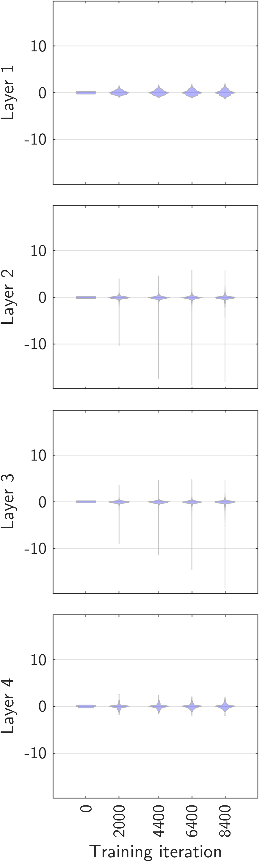
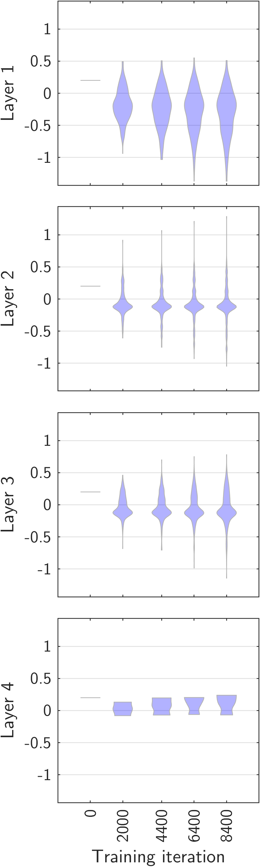
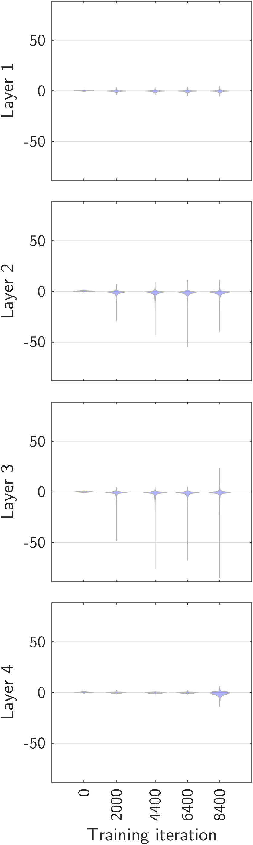
Figure 15: Distributions of the magnitudes of the weights, biases, and activations during training of a 3-layer MLP (the 4th row is the output layer) on the cameraman data. Weights and biases are initialized from a uniform distribution and zero, respectively. The distributions become very long-tailed as training progresses. The occurrence of large values is the reason why the dependence of the “preferred complexity” of certain architecture on weight magnitudes is important (it would not matter if the distribution of magnitudes remained constant throughout training).

	ReLU	GELU	Swish
Complexity (Fourier) $\longrightarrow$
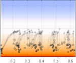
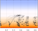
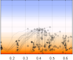
	TanH	Gaussian	Sine
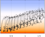
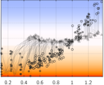
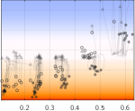
	Average magnitude of weights during training
	$\bullet$ At initialization     ▲ At last epoch    $\circ$ With shuffled trained weights
Lower frequenciesHigher frequencies

Figure 16: Training trajectories of MLP models trained on the cameraman data. Each line corresponds to one training run (with a different seed or initial weight magnitude). With ReLU-like activations, the models at initialization have low complexity regardless of the initialization magnitude. As training progresses, the complexity increases to fit the training data. This increased complexity is encoded in the weights precise values and connections across layers, since at the end of training, shuffling the weights reverts models to the initial low complexity. With other activations, the initial weight magnitude impacts the complexity at initialization and of the trained model. Some of the additional complexity in the trained model seems to be partly encoded by increases in the weight magnitudes, since shuffling the trained weights does seem to retain some of this additional complexity.

E.2 Training Trajectories

We will now show that NNs can represent any function, but complex ones require precise weight values and connections across layers that are unlikely through random sampling but that can be found through gradient-based training.

Unlike prior work [59] that claimed that the complexity at initialization causally influences the solution, our results indicate instead they are two effects of a common cause (the “preferred complexity” of the architecture). The architecture is biased towards a certain complexity, and this influences both the randomly-initialized model and those found by gradient descent. There exist weight values for other functions (of complexity much lower or higher than the preferred one) but they are less likely to occur in either case.

For example, ReLU networks are biased towards simplicity but can represent complex functions. Yet, contrary to [59], initializing gradient descent with such a complex function does not yield a complex solutions after training on simple data. In other words, the architecture’s bias prevails over the exact starting point of the training.

Experimental setup.

We train models with different activations and initial magnitudes on the cameraman data, using $\nicefrac{{1}}{{9}}$ pixels for training. We plot in Figure 16 the training trajectory of each model. Each point of a trajectory represents the average weight magnitude vs. the Fourier complexity of the function represented by the model.

Changes in weight magnitudes during training.

The first observation is that the average weight magnitude changes surprisingly little. However, further examination (Figure 15) shows that the distribution shifts from uniform to long-tailed. The trained models contain more and more large-magnitude weights.

Changes in complexity during training.

In Figure 16, we observe that models with ReLU-like activations at initialization have low complexity regardless of the initialization magnitude. As training progresses, the complexity increases to fit the training data. This increased complexity is encoded in the weights’ precise values and connections across layers, since at the end of training, shuffling the weights reverts models back to the initial low complexity. With other activations, the initial weight magnitudes impact the complexity at initialization and of the trained model. Some of the additional complexity in the trained model seems to be partly encoded by increases in weight magnitudes, since shuffling the trained weights does seem to retain some of this additional complexity.

Summary.

The choice of activation function and initial weight magnitude affect the “preferred complexity” of a model. This complexity is visible both at initialization (with random weights) and after training with gradient descent. The complexity of the learned function can depart from the “preferred level” just enough to fit the training points. Outside the interpolated training points, the shape of the learned function is very much affected by the preferred complexity.

With ReLU networks, this effect usually drives the complexity downwards (the simplicity bias). With other architectures and large weight magnitudes, this often drives the complexity upwards. Both can be useful: Section 4 showed that sine activations can enable learning the parity function from sparse training points, and reduce shortcut learning by shifting the preferred complexity upwards.

Our observations also explain why the coordinate-MLPs with sine activations proposed in [68] (SIREN) require a careful initialization. This adjusts the preferred complexity to the typical frequencies found in natural images.

E.3 Pretraining and Fine-tuning

We outline preliminary results from additional experiments.

Why study fine-tuning?

We have seen that the preferred complexity of an architecture can be observed with random weights. The model can then be trained by gradient descent to represent data with a different level of complexity. For example, a ReLU network, initially biased for simplicity, can represent a complex function after training on complex data. Gradient descent finely adjusts the weights to represent a complex function. We will now see how pretraining then fine-tuning on data with different levels of complexity “blends” the two in the final fine-tuned model.

Experimental setup.

We pretrain an MLP with ReLU or TanH activations on high-frequency data (high-frequency 2D sine waves). We then fine-tune it on lower-frequency 2D sine waves of a different random orientation.

Observations.

During early fine-tuning iterations, TanH models retain a high-frequency bias much more than ReLU models. This agrees with the proposition in E.1 that the former encode high frequencies in weight magnitudes, while ReLU models encode them in precise weight values, which are quickly lost during fine-tuning.

We further verify this explanation by shuffling the pretrained weights (within each layer) before fine-tuning. The ReLU models then show no high-frequency bias at all (since the precise arrangement of weights is completely lost through the shuffling). TanH models, however, do still show high-frequency components in the fine-tuned solution. This confirms that TanH models encode high frequencies partly in weight magnitudes since this is the only property preserved by the shuffling.

Finally, we do not find evidence for the prior claim [59] that complexity at initialization persists indefinitely throughout fine-tuning. Instead, with enough iterations of fine-tuning, any pretraining effect on the preferred complexity eventually vanishes. For example, a ReLU model pretrained on high frequencies initially contains high-frequency components in the fine-tuned model. But with enough iterations, they eventually disappear i.e. the simplicity bias of ReLUs eventually takes over. We believe that the experiments in [59] were simply not run for long enough. This observation also disproves the causal link proposed in [59] between the complexity at initialization and in the trained model.

Appendix F Full Results with Random Networks

On the next pages (Figures 19–21), we present heatmaps showing the average complexity of functions implemented by neural networks of various architectures with random weights and biases. Each heatmap corresponds to one architecture with varying number of layers (heatmap columns) and weight magnitudes (heatmap rows). For every other cell of a heatmap, we visualize, as a 2D grayscale image, a function implemented by one such a network with 2D input and scalar output.

	ReLU	GELU	Swish	SELU	TanH	Gaussian	Sin	Unbiased
Fourier
Chebyshev
Legendre
LZ

Figure 17: All measures of complexity (Y axes) of random networks generally increase with weight/activation magnitudes (X axis). The sensitivity is however very different across activation functions (columns). This sensitivity also increases with multiplicative interactions (i.e. gating), decreases with residual connections, and is essentially absent with layer normalization. These effects are also visible on the heatmaps (see next pages), but faint hence visualized here as line plots.

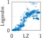
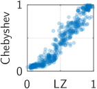
Figure 18: Correlations between our measures of complexity on random networks. They are based on frequency (Fourier), polynomial order (Legendre, Chebyshev), or compressibility (LZ). They capture different notions, yet they are closely correlated.

ReLU	GELU	Swish	SELU	TanH	Gaussian	Sin	Unbiased
With residual connections:
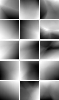
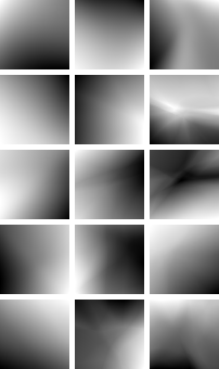
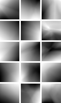
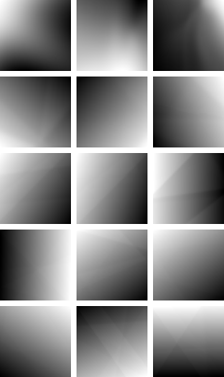
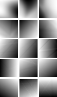
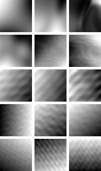
With layer normalization:
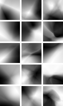
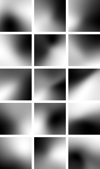
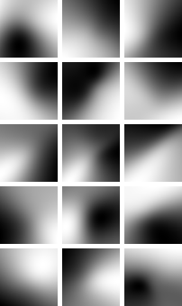
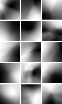
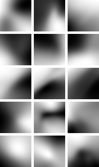
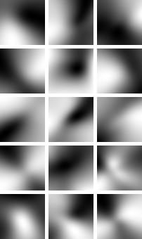
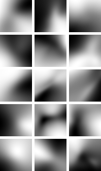
With gating:

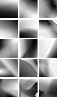
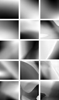
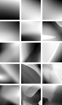
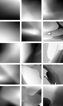
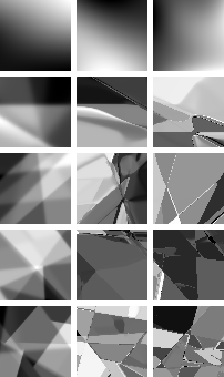
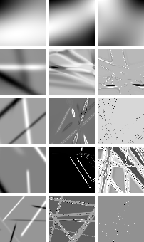
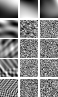
Figure 19: Heatmaps of the average complexity (Fourier) of various architectures with random weights, and example functions.

ReLU	GELU	Swish	SELU	TanH	Gaussian	Sin	Unbiased
With residual connections:
With layer normalization:
With gating:

Figure 20: Same as Figure 19 with the LZ measure instead of the Fourier-based one. Results are nearly identical.

ReLU	GELU	Swish	SELU	TanH	Gaussian	Sin	Unbiased
With residual connections:
With layer normalization:
With gating:

Figure 21: Same as Figure 19 with the LZ measure instead of the Fourier-based one. Results are nearly identical but noisier.

References

- Abbe et al. [2023] Emmanuel Abbe, Samy Bengio, Aryo Lotfi, and Kevin Rizk. Generalization on the unseen, logic reasoning and degree curriculum. arXiv preprint arXiv:2301.13105, 2023.
- Arora et al. [2019] Sanjeev Arora, Nadav Cohen, Wei Hu, and Yuping Luo. Implicit regularization in deep matrix factorization. NeurIPS, 32, 2019.
- Arpit et al. [2017] Devansh Arpit, Stanislaw Jastrzebski, Nicolas Ballas, David Krueger, Emmanuel Bengio, Maxinder S Kanwal, Tegan Maharaj, Asja Fischer, Aaron Courville, Yoshua Bengio, et al. A closer look at memorization in deep networks. In ICML, pages 233–242. PMLR, 2017.
- Ba et al. [2016] Jimmy Lei Ba, Jamie Ryan Kiros, and Geoffrey E Hinton. Layer normalization. arXiv preprint arXiv:1607.06450, 2016.
- Bachmann et al. [2023] Gregor Bachmann, Sotiris Anagnostidis, and Thomas Hofmann. Scaling MLPs: A tale of inductive bias. arXiv preprint arXiv:2306.13575, 2023.
- Balduzzi et al. [2017] David Balduzzi, Marcus Frean, Lennox Leary, JP Lewis, Kurt Wan-Duo Ma, and Brian McWilliams. The shattered gradients problem: If resnets are the answer, then what is the question? In International Conference on Machine Learning, pages 342–350. PMLR, 2017.
- Bhattamishra et al. [2022] Satwik Bhattamishra, Arkil Patel, Varun Kanade, and Phil Blunsom. Simplicity bias in transformers and their ability to learn sparse boolean functions. arXiv preprint arXiv:2211.12316, 2022.
- Boopathy et al. [2023] Akhilan Boopathy, Kevin Liu, Jaedong Hwang, Shu Ge, Asaad Mohammedsaleh, and Ila R Fiete. Model-agnostic measure of generalization difficulty. In ICML, pages 2857–2884. PMLR, 2023.
- Chiang et al. [2022] Ping-yeh Chiang, Renkun Ni, David Yu Miller, Arpit Bansal, Jonas Geiping, Micah Goldblum, and Tom Goldstein. Loss landscapes are all you need: Neural network generalization can be explained without the implicit bias of gradient descent. In ICLR, 2022.
- Choraria et al. [2022] Moulik Choraria, Leello Tadesse Dadi, Grigorios Chrysos, Julien Mairal, and Volkan Cevher. The spectral bias of polynomial neural networks. arXiv preprint arXiv:2202.13473, 2022.
- Cohen and Shashua [2016] Nadav Cohen and Amnon Shashua. Inductive bias of deep convolutional networks through pooling geometry. arXiv preprint arXiv:1605.06743, 2016.
- De Palma et al. [2019] Giacomo De Palma, Bobak Kiani, and Seth Lloyd. Random deep neural networks are biased towards simple functions. NeurIPS, 32, 2019.
- Delétang et al. [2022] Grégoire Delétang, Anian Ruoss, Jordi Grau-Moya, Tim Genewein, Li Kevin Wenliang, Elliot Catt, Chris Cundy, Marcus Hutter, Shane Legg, Joel Veness, et al. Neural networks and the chomsky hierarchy. arXiv preprint arXiv:2207.02098, 2022.
- Dherin et al. [2022] Benoit Dherin, Michael Munn, Mihaela Rosca, and David Barrett. Why neural networks find simple solutions: The many regularizers of geometric complexity. NeurIPS, 35:2333–2349, 2022.
- Dingle et al. [2018] Kamaludin Dingle, Chico Q Camargo, and Ard A Louis. Input–output maps are strongly biased towards simple outputs. Nature communications, 9(1):761, 2018.
- Dubey et al. [2022] Shiv Ram Dubey, Satish Kumar Singh, and Bidyut Baran Chaudhuri. Activation functions in deep learning: A comprehensive survey and benchmark. Neurocomputing, 2022.
- Entezari et al. [2021] Rahim Entezari, Hanie Sedghi, Olga Saukh, and Behnam Neyshabur. The role of permutation invariance in linear mode connectivity of neural networks. arXiv preprint arXiv:2110.06296, 2021.
- Francazi et al. [2023] Emanuele Francazi, Aurelien Lucchi, and Marco Baity-Jesi. Initial guessing bias: How untrained networks favor some classes. arXiv preprint arXiv:2306.00809, 2023.
- Frankle et al. [2020] Jonathan Frankle, Gintare Karolina Dziugaite, Daniel Roy, and Michael Carbin. Linear mode connectivity and the lottery ticket hypothesis. In International Conference on Machine Learning, pages 3259–3269. PMLR, 2020.
- Frei et al. [2022] Spencer Frei, Gal Vardi, Peter L Bartlett, Nathan Srebro, and Wei Hu. Implicit bias in leaky relu networks trained on high-dimensional data. arXiv preprint arXiv:2210.07082, 2022.
- Fu et al. [2021] Zihao Fu, Wai Lam, Anthony Man-Cho So, and Bei Shi. A theoretical analysis of the repetition problem in text generation. In AAAI, pages 12848–12856, 2021.
- Gallant [1988] Gallant. There exists a neural network that does not make avoidable mistakes. In IEEE International Conference on Neural Networks, pages 657–664. IEEE, 1988.
- Garriga-Alonso et al. [2018] Adrià Garriga-Alonso, Carl Edward Rasmussen, and Laurence Aitchison. Deep convolutional networks as shallow gaussian processes. arXiv preprint arXiv:1808.05587, 2018.
- Geiping et al. [2021] Jonas Geiping, Micah Goldblum, Phillip E Pope, Michael Moeller, and Tom Goldstein. Stochastic training is not necessary for generalization. arXiv preprint arXiv:2109.14119, 2021.
- Geirhos et al. [2020] Robert Geirhos, Jörn-Henrik Jacobsen, Claudio Michaelis, Richard Zemel, Wieland Brendel, Matthias Bethge, and Felix A Wichmann. Shortcut learning in deep neural networks. Nature Machine Intelligence, 2(11):665–673, 2020.
- Gilkes [1974] Alan Martin Gilkes. Photograph enhancement by adaptive digital unsharp masking. PhD thesis, Massachusetts Institute of Technology, 1974.
- Giryes et al. [2016] Raja Giryes, Guillermo Sapiro, and Alex M Bronstein. Deep neural networks with random gaussian weights: A universal classification strategy? IEEE Transactions on Signal Processing, 64(13):3444–3457, 2016.
- Glorot and Bengio [2010] Xavier Glorot and Yoshua Bengio. Understanding the difficulty of training deep feedforward neural networks. In International Conference on Artificial Intelligence and Statistics, pages 249–256. JMLR, 2010.
- Goldblum et al. [2023] Micah Goldblum, Marc Finzi, Keefer Rowan, and Andrew Gordon Wilson. The no free lunch theorem, kolmogorov complexity, and the role of inductive biases in machine learning. arXiv preprint arXiv:2304.05366, 2023.
- Hahn et al. [2021] Michael Hahn, Dan Jurafsky, and Richard Futrell. Sensitivity as a complexity measure for sequence classification tasks. Transactions of the ACL, 9:891–908, 2021.
- He et al. [2016] Kaiming He, Xiangyu Zhang, Shaoqing Ren, and Jian Sun. Deep residual learning for image recognition. In CVPR, pages 770–778, 2016.
- Hermann and Lampinen [2020] Katherine L Hermann and Andrew K Lampinen. What shapes feature representations? exploring datasets, architectures, and training. arXiv preprint arXiv:2006.12433, 2020.
- Hermann et al. [2023] Katherine L Hermann, Hossein Mobahi, Thomas Fel, and Michael C Mozer. On the foundations of shortcut learning. arXiv preprint arXiv:2310.16228, 2023.
- Holtzman et al. [2019] Ari Holtzman, Jan Buys, Li Du, Maxwell Forbes, and Yejin Choi. The curious case of neural text degeneration. arXiv preprint arXiv:1904.09751, 2019.
- Hong et al. [2022] Qingguo Hong, Jonathan W Siegel, Qinyang Tan, and Jinchao Xu. On the activation function dependence of the spectral bias of neural networks. arXiv preprint arXiv:2208.04924, 2022.
- Hornik et al. [1989] Kurt Hornik, Maxwell Stinchcombe, and Halbert White. Multilayer feedforward networks are universal approximators. Neural networks, 2(5):359–366, 1989.
- Huang et al. [2020] W. Ronny Huang, Zeyad Emam, Micah Goldblum, Liam Fowl, Justin K. Terry, Furong Huang, and Tom Goldstein. Understanding generalization through visualizations. In ”I Can’t Believe It’s Not Better!” NeurIPS Workshop, pages 87–97. PMLR, 2020.
- Huh et al. [2021] Minyoung Huh, Hossein Mobahi, Richard Zhang, Brian Cheung, Pulkit Agrawal, and Phillip Isola. The low-rank simplicity bias in deep networks. arXiv preprint arXiv:2103.10427, 2021.
- Jayakumar et al. [2020] Siddhant M Jayakumar, Wojciech M Czarnecki, Jacob Menick, Jonathan Schwarz, Jack Rae, Simon Osindero, Yee Whye Teh, Tim Harley, and Razvan Pascanu. Multiplicative interactions and where to find them. In ICLR, 2020.
- Lee et al. [2017] Jaehoon Lee, Yasaman Bahri, Roman Novak, Samuel S Schoenholz, Jeffrey Pennington, and Jascha Sohl-Dickstein. Deep neural networks as gaussian processes. arXiv preprint arXiv:1711.00165, 2017.
- Lyu et al. [2021] Kaifeng Lyu, Zhiyuan Li, Runzhe Wang, and Sanjeev Arora. Gradient descent on two-layer nets: Margin maximization and simplicity bias. NeurIPS, 34:12978–12991, 2021.
- Maas et al. [2013] Andrew L Maas, Awni Y Hannun, Andrew Y Ng, et al. Rectifier nonlinearities improve neural network acoustic models. In ICML, page 3. Atlanta, GA, 2013.
- Matthews et al. [2018] Alexander G de G Matthews, Mark Rowland, Jiri Hron, Richard E Turner, and Zoubin Ghahramani. Gaussian process behaviour in wide deep neural networks. In ICLR, 2018.
- Mingard et al. [2019] Chris Mingard, Joar Skalse, Guillermo Valle-Pérez, David Martínez-Rubio, Vladimir Mikulik, and Ard A Louis. Neural networks are a priori biased towards boolean functions with low entropy. arXiv preprint arXiv:1909.11522, 2019.
- Mitchell [1980] Tom M Mitchell. The need for biases in learning generalizations. Rutgers University CS tech report CBM-TR-117, 1980.
- Mohtashami et al. [2023] Amirkeivan Mohtashami, Martin Jaggi, and Sebastian U Stich. Special properties of gradient descent with large learning rates. arXiv preprint arXiv:2205.15142, 2023.
- Montufar et al. [2014] Guido F Montufar, Razvan Pascanu, Kyunghyun Cho, and Yoshua Bengio. On the number of linear regions of deep neural networks. NeurIPS, 27, 2014.
- Neyshabur et al. [2014] Behnam Neyshabur, Ryota Tomioka, and Nathan Srebro. In search of the real inductive bias: On the role of implicit regularization in deep learning. arXiv preprint arXiv:1412.6614, 2014.
- Oostwal et al. [2021] Elisa Oostwal, Michiel Straat, and Michael Biehl. Hidden unit specialization in layered neural networks: Relu vs. sigmoidal activation. Physica A: Statistical Mechanics and its Applications, 564:125517, 2021.
- Pennington et al. [2018] Jeffrey Pennington, Samuel Schoenholz, and Surya Ganguli. The emergence of spectral universality in deep networks. In International Conference on Artificial Intelligence and Statistics, pages 1924–1932. PMLR, 2018.
- Pesme et al. [2021] Scott Pesme, Loucas Pillaud-Vivien, and Nicolas Flammarion. Implicit bias of sgd for diagonal linear networks: a provable benefit of stochasticity. NeurIPS, 34:29218–29230, 2021.
- Pezeshki et al. [2021] Mohammad Pezeshki, Oumar Kaba, Yoshua Bengio, Aaron C Courville, Doina Precup, and Guillaume Lajoie. Gradient starvation: A learning proclivity in neural networks. NeurIPS, 34:1256–1272, 2021.
- Poggio et al. [2018] Tomaso Poggio, Kenji Kawaguchi, Qianli Liao, Brando Miranda, Lorenzo Rosasco, Xavier Boix, Jack Hidary, and Hrushikesh Mhaskar. Theory of deep learning III: the non-overfitting puzzle. CBMM Memo, 73:1–38, 2018.
- Poole et al. [2016] Ben Poole, Subhaneil Lahiri, Maithra Raghu, Jascha Sohl-Dickstein, and Surya Ganguli. Exponential expressivity in deep neural networks through transient chaos. NeurIPS, 29, 2016.
- Radford et al. [2019] Alec Radford, Jeffrey Wu, Rewon Child, David Luan, Dario Amodei, Ilya Sutskever, et al. Language models are unsupervised multitask learners. OpenAI blog, 1(8):9, 2019.
- Raghu et al. [2017] Maithra Raghu, Ben Poole, Jon Kleinberg, Surya Ganguli, and Jascha Sohl-Dickstein. On the expressive power of deep neural networks. In ICML, pages 2847–2854. PMLR, 2017.
- Rahaman et al. [2019] Nasim Rahaman, Aristide Baratin, Devansh Arpit, Felix Draxler, Min Lin, Fred Hamprecht, Yoshua Bengio, and Aaron Courville. On the spectral bias of neural networks. In ICML, pages 5301–5310. PMLR, 2019.
- Ramasinghe and Lucey [2022] Sameera Ramasinghe and Simon Lucey. Beyond periodicity: Towards a unifying framework for activations in coordinate-MLPs. In ECCV, pages 142–158. Springer, 2022.
- Ramasinghe et al. [2022a] Sameera Ramasinghe, Lachlan MacDonald, Moshiur Farazi, Hemanth Saratchandran, and Simon Lucey. How you start matters for generalization. arXiv preprint arXiv:2206.08558, 2022a.
- Ramasinghe et al. [2022b] Sameera Ramasinghe, Lachlan E MacDonald, and Simon Lucey. On the frequency-bias of coordinate-MLPs. NeurIPS, 35:796–809, 2022b.
- Saragadam et al. [2023] Vishwanath Saragadam, Daniel LeJeune, Jasper Tan, Guha Balakrishnan, Ashok Veeraraghavan, and Richard G Baraniuk. Wire: Wavelet implicit neural representations. In CVPR, pages 18507–18516, 2023.
- Schmidhuber [1997] Jürgen Schmidhuber. Discovering neural nets with low kolmogorov complexity and high generalization capability. Neural Networks, 10(5):857–873, 1997.
- Schoenholz et al. [2016] Samuel S Schoenholz, Justin Gilmer, Surya Ganguli, and Jascha Sohl-Dickstein. Deep information propagation. arXiv preprint arXiv:1611.01232, 2016.
- Scimeca et al. [2021] Luca Scimeca, Seong Joon Oh, Sanghyuk Chun, Michael Poli, and Sangdoo Yun. Which shortcut cues will dnns choose? a study from the parameter-space perspective. arXiv preprint arXiv:2110.03095, 2021.
- Shah et al. [2020] Harshay Shah, Kaustav Tamuly, Aditi Raghunathan, Prateek Jain, and Praneeth Netrapalli. The pitfalls of simplicity bias in neural networks. NeurIPS, 33:9573–9585, 2020.
- Shalev-Shwartz et al. [2017] Shai Shalev-Shwartz, Ohad Shamir, and Shaked Shammah. Failures of gradient-based deep learning. In ICML, pages 3067–3075. PMLR, 2017.
- Simon et al. [2022] James Benjamin Simon, Sajant Anand, and Mike Deweese. Reverse engineering the neural tangent kernel. In ICML, pages 20215–20231. PMLR, 2022.
- Sitzmann et al. [2020] Vincent Sitzmann, Julien Martel, Alexander Bergman, David Lindell, and Gordon Wetzstein. Implicit neural representations with periodic activation functions. NeurIPS, 33:7462–7473, 2020.
- Smith et al. [2021] Samuel L Smith, Benoit Dherin, David GT Barrett, and Soham De. On the origin of implicit regularization in stochastic gradient descent. arXiv preprint arXiv:2101.12176, 2021.
- Soudry et al. [2018] Daniel Soudry, Elad Hoffer, Mor Shpigel Nacson, Suriya Gunasekar, and Nathan Srebro. The implicit bias of gradient descent on separable data. The Journal of Machine Learning Research, 19(1):2822–2878, 2018.
- Stock et al. [2022] Joshua Stock, Jens Wettlaufer, Daniel Demmler, and Hannes Federrath. Property unlearning: A defense strategy against property inference attacks. arXiv preprint arXiv:2205.08821, 2022.
- Sutton [2019] Richard Sutton. The bitter lesson. Incomplete Ideas (blog), 13(1), 2019.
- Tachet et al. [2018] Remi Tachet, Mohammad Pezeshki, Samira Shabanian, Aaron Courville, and Yoshua Bengio. On the learning dynamics of deep neural networks. arXiv preprint arXiv:1809.06848, 2018.
- Tancik et al. [2020] Matthew Tancik, Pratul Srinivasan, Ben Mildenhall, Sara Fridovich-Keil, Nithin Raghavan, Utkarsh Singhal, Ravi Ramamoorthi, Jonathan Barron, and Ren Ng. Fourier features let networks learn high frequency functions in low dimensional domains. NeurIPS, 33:7537–7547, 2020.
- Teney et al. [2021] Damien Teney, Ehsan Abbasnejad, Simon Lucey, and Anton van den Hengel. Evading the simplicity bias: Training a diverse set of models discovers solutions with superior ood generalization. arXiv preprint arXiv:2105.05612, 2021.
- Teney et al. [2022] Damien Teney, Maxime Peyrard, and Ehsan Abbasnejad. Predicting is not understanding: Recognizing and addressing underspecification in machine learning. In European Conference on Computer Vision, pages 458–476. Springer, 2022.
- Theisen et al. [2021] Ryan Theisen, Jason Klusowski, and Michael Mahoney. Good classifiers are abundant in the interpolating regime. In AISTATS, pages 3376–3384. PMLR, 2021.
- Ulyanov et al. [2018] Dmitry Ulyanov, Andrea Vedaldi, and Victor Lempitsky. Deep image prior. In CVPR, pages 9446–9454, 2018.
- Valle-Perez et al. [2018] Guillermo Valle-Perez, Chico Q Camargo, and Ard A Louis. Deep learning generalizes because the parameter-function map is biased towards simple functions. arXiv preprint arXiv:1805.08522, 2018.
- Vardi [2023] Gal Vardi. On the implicit bias in deep-learning algorithms. Communications of the ACM, 66(6):86–93, 2023.
- Xie et al. [2022] Yiheng Xie, Towaki Takikawa, Shunsuke Saito, Or Litany, Shiqin Yan, Numair Khan, Federico Tombari, James Tompkin, Vincent Sitzmann, and Srinath Sridhar. Neural fields in visual computing and beyond. In Computer Graphics Forum, pages 641–676. Wiley Online Library, 2022.
- Xiong et al. [2020] Ruibin Xiong, Yunchang Yang, Di He, Kai Zheng, Shuxin Zheng, Chen Xing, Huishuai Zhang, Yanyan Lan, Liwei Wang, and Tieyan Liu. On layer normalization in the transformer architecture. In International Conference on Machine Learning, pages 10524–10533. PMLR, 2020.
- Xu et al. [2019a] Jingjing Xu, Xu Sun, Zhiyuan Zhang, Guangxiang Zhao, and Junyang Lin. Understanding and improving layer normalization. Advances in Neural Information Processing Systems, 32, 2019a.
- Xu et al. [2019b] Zhi-Qin John Xu, Yaoyu Zhang, Tao Luo, Yanyang Xiao, and Zheng Ma. Frequency principle: Fourier analysis sheds light on deep neural networks. arXiv preprint arXiv:1901.06523, 2019b.
- Xu et al. [2019c] Zhi-Qin John Xu, Yaoyu Zhang, and Yanyang Xiao. Training behavior of deep neural network in frequency domain. In ICONIP, pages 264–274. Springer, 2019c.
- Yang and Salman [2019] Greg Yang and Hadi Salman. A fine-grained spectral perspective on neural networks. arXiv preprint arXiv:1907.10599, 2019.
- Zhang et al. [2023a] Enyan Zhang, Michael A Lepori, and Ellie Pavlick. Instilling inductive biases with subnetworks. arXiv preprint arXiv:2310.10899, 2023a.
- Zhang et al. [2023b] Shijun Zhang, Hongkai Zhao, Yimin Zhong, and Haomin Zhou. Why shallow networks struggle with approximating and learning high frequency: A numerical study. arXiv preprint arXiv:2306.17301, 2023b.
- Zhou et al. [2023a] Allan Zhou, Kaien Yang, Kaylee Burns, Yiding Jiang, Samuel Sokota, J Zico Kolter, and Chelsea Finn. Permutation equivariant neural functionals. arXiv preprint arXiv:2302.14040, 2023a.
- Zhou et al. [2023b] Hattie Zhou, Arwen Bradley, Etai Littwin, Noam Razin, Omid Saremi, Josh Susskind, Samy Bengio, and Preetum Nakkiran. What algorithms can transformers learn? a study in length generalization. arXiv preprint arXiv:2310.16028, 2023b.