Transformers Provably Learn Feature-Position Correlations in Masked Image Modeling

Abstract

Masked image modeling (MIM), which predicts randomly masked patches from unmasked ones, has emerged as a promising approach in self-supervised vision pretraining. However, the theoretical understanding of MIM is rather limited, especially with the foundational architecture of transformers. In this paper, to the best of our knowledge, we provide the first end-to-end theory of learning one-layer transformers with softmax attention in MIM self-supervised pretraining. On the conceptual side, we posit a theoretical mechanism of how transformers, pretrained with MIM, produce empirically observed local and diverse attention patterns on data distributions with spatial structures that highlight feature-position correlations. On the technical side, our end-to-end analysis of the training dynamics of softmax-based transformers accommodates both input and position embeddings simultaneously, which is developed based on a novel approach to track the interplay between the attention of feature-position and position-wise correlations.

1 Introduction

Self-supervised learning has been the dominant approach to pretrain neural networks for downstream applications since the introduction of BERT [12] and GPT [37] in natural language processing (NLP). On the side of vision, self-supervised learning was initially more focused on the discriminative methods, which include contrastive learning [21, 5] and non-contrastive learning methods [16, 5, 8, 61]. Inspired by the masked language models in NLP, and also due to the crucial progress by [11] in successfully implementing vision transformers (ViTs), the generative approach of self-supervised learning, such as masked image modeling (MIM), has become popular in self-supervised vision pretraining, especially due to the rise of masked auto-encoder (MAE) [20] and SimMIM [58].

In MIM, neural network are instructed to reconstruct some or all parts of an image given a masked version, aiming to learn certain abstract semantics of visual contents when trained to fill in the missing pixels. In practice, this approach not only proves to be very successful but also unveils intriguing phenomena that diverge significantly from the behaviors observed in other self-supervised learning approaches. The initial work of [20] showed that MAE can conduct visual reasoning when filling in masked patches even with very high mask rates, suggesting that MIM learns not only global representations but also complex relationships between visual objects and shapes. Some critical observations from recent research [53, 33, 57] have suggested that the models trained via MIM display diverse locality inductive bias, contrasting with the uniform long-range global patterns typically emphasized by other discriminative self-supervised learning approaches.

Despite the great empirical effort put into investigating the MIM, our theoretical understanding of MIM is still nascent. Most existing theories for self-supervised learning focused on discriminative methods [2, 7, 38, 22, 54, 43, 50, 55], such as contrastive learning. Among very few attempts towards MIM, [9] studied the patch-based attention via an integral kernel perspective; [62] analyzed MAE through an augmentation graph framework, which connects MAE with contrastive learning. [35] characterized the optimization process of MAE with shallow convolutional neural networks (CNNs). Nonetheless, transformer, the dominant architecture in current deep learning practice, was not touched upon in the above theoretical studies of MIM and, more broadly, self-supervised learning methods, leaving a considerable vacuum in the literature.

Building on the mind-blowing empirical advances and recognizing the lack of theoretical understanding of MIM and transformers in self-supervised learning, we are motivated to answer the following intriguing question: Can we theoretically characterize what solution the transformer converges to in MIM? How does the MIM optimize the transformer to learn diverse local patterns instead of the collapsed global solution?

Contributions.

In this paper, we take a first step towards answering the above question, and highlight our contributions below.

1. We give, to our knowledge, the first end-to-end theory of learning one-layer transformers with softmax attention in masked-reconstruction type self-supervised pretraining, in terms of global convergence guarantee of the loss function trained by gradient descent (GD).

2. We analyze the feature learning process of one-layer transformers on data distributions with spatial structures that highlight feature-position correlations, to characterize attention patterns at the time of convergence of MIM. To our knowledge, this marks the first result of the learning of softmax self-attention model that jointly considers both input and position encodings.

3. Our theoretical proofs and new empirical observations (cf. Figure 3), collectively provide an explanation to the local and diverse attention patterns observed from MIM pretraining [33, 57]. We design a novel empirical metric, attention diversity metric, to probe vision transformers trained by different methods. We show that trained masked image models, due to the nature of their reconstruction training objectives, are capable of attending to visual features irrespective of their significance.

Comparisons with prior works.

A few works [23, 35] have studied topics that are related to ours. Here we summarize the differences of our work from theirs in terms of settings and analysis at a high level. In Section 3.1, after formally defining the feature-position correlations, we will address the limitations of previous works, particularly their inadequacy to fully capture MIM’s capability to learn locality, from a more technical perspective.

• [23] is the first work to characterize the training dynamics of transformers in supervised learning. They provided the first convergence result for one-layer softmax-attention transformers trained on a simple visual data distribution, in which the partition of patches is fixed (see Definition 2.1 in their paper). Their assumptions require learning only the position-position correlations (see Definition 3.1) in the softmax attention, which is rather limited. We draw inspiration from their data assumptions and generalize them to allow variable partitions of patches (see Definition 2.1) with different spatial structures. Because of this generalization, we need to analyze the learning processes of different spatial correlations among visual features simultaneously, which poses key challenges in the overall analysis.

• [35] proved a feature-learning result for MAEs with CNNs rather than transformers, on the so-called multi-view data [3] for proving the superiority of learned features. Although both our and their works focus on the dynamics of gradient descent, since our work needs to handle transformers and patch-wise data distribution, which are not present in their study, our analysis techniques are significantly different from theirs.

Notation.

We introduce notation to be used throughout the paper. For any two functions $h(x)$ and $g(x)$, we employ the notation $h(x)=\Omega(g(x))$ $\big{(}$resp. $h(x)=O(g(x))\big{)}$ to denote that there exist some universal constants $C_{1}>0$ and $a_{1}$, s.t. $|h(x)|\geq C_{1}|g(x)|$ $\big{(}$resp. $|h(x)|\leq C_{1}|g(x)|\big{)}$ for all $x\geq a_{1}$; Furthermore, $h(x)=\Theta(g(x))$ indicates $h(x)=\Omega(g(x))$ and $h(x)=O(g(x))$ hold simultaneously. We use $\operatorname{\mathds{1}}\{\cdot\}$ to denote the indicator function. Let $[N]\coloneqq\{1,2,\ldots,N\}$. We use $\widetilde{O}$, $\widetilde{\Omega}$, and $\widetilde{\Theta}$ to further hide logarithmic factors in the respective order notation. We use $\operatorname{poly}(P)$ and $\operatorname{polylog}(P)$ to represent large constant-degree polynomials of $P$ and $\log(P)$, respectively.

2 Problem Setup

In this section, we present our problem formulations to study the training process of transformers with MIM pretraining. We first provide some background, and then introduce our dataset setting and present the MIM pretraining strategy with the transformer architecture we consider in this paper.

2.1 Masked Image Reconstruction

We follow the MIM frameworks in [20, 58]. Each data sample $X\in\mathbb{R}^{d\times P}$ has the form $X=(X_{\mathbf{p}})_{\mathbf{p}\in\mathcal{P}}$, which has $|\mathcal{P}|=P$ patches, and each patch $X_{\mathbf{p}}\in\mathbb{R}^{d}$. Given a collection of images $\{X_{i}\}_{i\in[n]}$, we select a masking set $\mathcal{M}\subset[P]$ and mask them by setting the masked patches to some $\mathsf{M}\in\mathbb{R}^{d}$, leading to masked images $\{\mathsf{M}(X_{i})\}_{i\in[n]}$, where

$$\mathsf{M}(X_{i})_{\mathbf{p}}=\left\{\begin{array}[]{cc}[X_{i}]_{\mathbf{p}}&\mathbf{p}\in\mathcal{U}\\ \mathsf{M}&\mathbf{p}\in\mathcal{M}\end{array}\right.,\qquad i\in[n],$$ (2.3)

where $\mathcal{U}$ is the index set of unmasked patches. Let $F:X\mapsto\widehat{X}$ be a neural network that outputs a reconstructed image $\widehat{X}\in\mathbb{R}^{d\times P}$ for any given input $X\in\mathbb{R}^{d\times P}$. The pretraining objective can then be set as a mean-squared reconstruction loss of a subset $\mathcal{P}^{\prime}\subset\mathcal{P}$ of the image as follows:

$$\mathcal{L}(F)=\frac{1}{n}\sum_{i=1}^{n}\sum_{\mathbf{p}\in\mathcal{P}^{\prime}}\Big{\|}[X_{i}]_{\mathbf{p}}-[F(\mathsf{M}(X_{i}))]_{\mathbf{p}}\Big{\|}_{2}^{2}.$$

In [20] the chosen subset $\mathcal{P}^{\prime}$ is the set of masked patches $\mathcal{M}$, while [58] chose to reconstruct the full image $\mathcal{P}^{\prime}=\mathcal{P}$. Here we do not study the trade-off between the two formulations. As shall be seen momentarily, we base our theory upon a simplified version of vision transformers [11] which utilizes the attention mechanism [49].

2.2 Data Distribution

We assume the data samples $X\in\mathbb{R}^{d\times P}$ are drawn independently from some data distribution $\mathcal{D}$. To capture the feature-position (FP) correlation in the learning problem, we consider the following setup for the vision data. Specifically, we assume that the data distribution consists of many different clusters, each defined by a different partition of patches and a different set of visual features. We define the data distribution $\mathcal{D}$ formally as follows.

Definition 2.1 (Data distribution $\mathcal{D}$).

The data distribution $\mathcal{D}$ has $K=O(1)$ different clusters $\{\mathcal{D}_{k}\}_{k=1}^{K}$. For every cluster $\mathcal{D}_{k},k\in[K]$, there is a corresponding partition of $\mathcal{P}$ into $N_{k}$ disjoint subsets $\mathcal{P}=\bigcup^{N_{k}}_{j=1}\mathcal{P}_{k,j}$ which we call areas. For each sample $X=(X_{\mathbf{p}})_{\mathbf{p}\in\mathcal{P}}$, its sampling process is as follows:

• We draw $\mathcal{D}_{k}$ uniformly at random from all clusters and draw a sample $X$ from $\mathcal{D}_{k}$.

• Given $k\in[K]$, for any $j\in[N_{k}]$, all patches $X_{\mathbf{p}}$ in the area $\mathcal{P}_{k,j}$ are given the same content $X_{\mathbf{p}}=v_{k,j}z_{j}(X)$, where $v_{k,j}\in\mathbb{R}^{d}$ is the visual feature and $z_{j}(X)$ is the latent variable. We assume $\bigcup_{k=1}^{K}\bigcup^{N_{k}}_{j=1}\{v_{k,j}\}$ are orthogonal to each other with unit norm.

• Given $k\in[K]$, for any $j\in[N_{k}]$, $z_{j}(X)\in[L,U]$, where $0\leq L<U$ are on the order of $\Theta(1)$. The distribution of $z_{j}(X)$ can be arbitrary within the above support set.

Global and local features in an image.

In vision data, images inherently contain two distinct types of features: global features and local features. For instance, in an image of an object, global features can capture the shape and texture of the object, such as the fur color of an animal, whereas local features describe specific details of local areas, such as the texture of leaves in the background. Recent empirical studies on self-supervised pretraining with transformers [33, 53], have demonstrated that contrastive learning predominantly utilizes these globally projected representations to contrast each other. This often leads to a phenomenon known as “attention collapse”, where the attention maps for query patches from two different spatial locations surprisingly indicate identical object shapes. In contrast, MIM exhibits the capacity to avoid such collapse by identifying diverse local attention patterns for different query patches. Consequently, unraveling the mechanisms behind MIM necessitates a thorough examination of data characteristics that embody both global and local features.

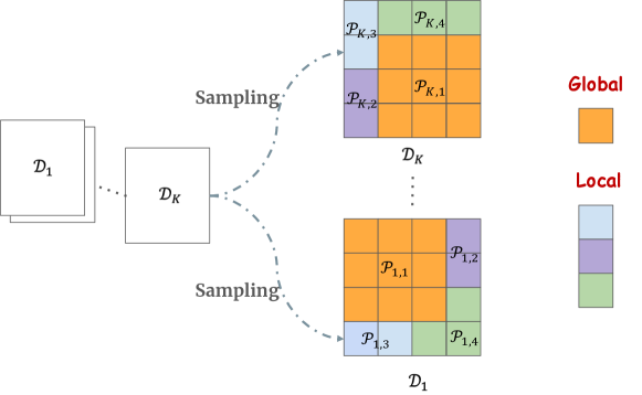
Figure 1: Illustration of the data distribution. Each cluster $\mathcal{D}_{k}$ is segmented into distinct areas $\mathcal{P}_{k,j}$ as in Definition 2.1, with squares in the same color representing the same area $\mathcal{P}_{k,j}$. The global region $\mathcal{P}_{k,1}$ (depicted in orange) contains a larger count of patches compared to any other local regions.

In this paper, we characterize these two types of features by the following assumption on the data.

Assumption 2.2 (Global feature vs local feature).

Let $\mathcal{D}_{k}\in[K]$ be a cluster from $\mathcal{D}$. We let $\mathcal{P}_{k,1}$ be the global area of cluster $\mathcal{D}_{k}$, and all the other areas $\mathcal{P}_{k,j},j\in[N_{k}]\setminus\{1\}$ be the local areas. Since each area corresponds to an assigned feature, we also call them the global and local features, respectively. Moreover, we assume:

• Global area: given $k\in[K]$, we assume $C_{k,1}=|\mathcal{P}_{k,1}|=\Theta(P^{\kappa_{c}})$ with $\kappa_{c}\in[0.5005,1]$, where $C_{k,1}$ is the number of patches in the global area $\mathcal{P}_{k,1}$.

• Local area: given $k\in[K]$, we choose $C_{k,j}=\Theta(P^{\kappa_{s}})$ with $\kappa_{s}\in[0.001,0.5]$ for $j>1$, where $C_{k,j}$ denotes the number of patches in the local area $\mathcal{P}_{k,j}$.

The rationale behind defining the global feature in this manner is based on the observation that the occurrence of patches depicting global features ($C_{k,1}$) are typically significantly higher than those of local features ($C_{k,j}$, for $j>1$), since global features tend to capture the main visual information in an image and provide a dominant view, whereas local features only describe small details within the image. An intuitive illustration of data generation is given in Figure 1.

2.3 Masked Image Modeling with Transformers

Transformer architecture.

A transformer block [49] consists of a self-attention layer and an MLP layer. The self-attention layer has multiple heads, each of which consists of the following components: a query matrix $W^{Q}$, a key matrix $W^{K}$, and a value matrix $W^{V}$. Given an input $X$, the self-attention layer is a mapping given as follows:

$$G(X;W^{Q},W^{K},W^{V})=W^{V}X\cdot\operatorname{softmax}\left({(W^{K}X)^{\top}W^{Q}X}\right),$$ (2.4)

where the $\operatorname{softmax}(\cdot)$ function is applied column-wise.

Since input tokens in transformers are indistinguishable without any proper positional structure, one should add positional encodings to the input embeddings in the softmax attention as in [23]. We state our assumption of the positional encodings as follows.

Assumption 2.3 (Positional encoding).

We assume fixed positional encodings: $E=(e_{{\mathbf{p}}})_{{\mathbf{p}}\in\mathcal{P}}\in\mathbb{R}^{d\times P}$ where positional embedding vectors $e_{{\mathbf{p}}}$ are orthogonal to each other and to all the features $v_{k,j}$, and are of unit-norm.

We now present the actual network architecture in the paper. To simplify the theoretical analysis, we consolidate the product of query and key matrices $(W^{K})^{\top}W^{Q}$ into one weight matrix denoted as $Q$. Furthermore, we set $W^{V}$ to be the identity matrix and fixed during the training. These simplifications are often taken in recent theoretical works [23, 19, 60], to allow tractable theoretical analysis. With these simplifications in place, (2.4) can be rewritten as

$$F(X;Q)=X\cdot\operatorname{softmax}\left({X^{\top}QX}\right),$$ (2.5)

which will be used for masked reconstruction, as formalized below.

Assumption 2.4 (Transformer network for MIM).

We assume that our vision transformer $F(X;Q)$ consists of a single self-attention layer with an attention weight matrix $Q\in\mathbb{R}^{d\times d}$. For an input image $X\sim\mathcal{D}$, we add positional encoding by $\widetilde{X}=X+E$. The attention score from patch $X_{\mathbf{p}}$ to patch $X_{{\mathbf{q}}}$ is denoted by

$$\textstyle\mathbf{attn}_{{\mathbf{p}}\to{\mathbf{q}}}(X;Q)\coloneqq\frac{e^{\widetilde{X}_{{\mathbf{p}}}^{\top}Q\widetilde{X}_{{\mathbf{q}}}}}{\sum_{{\mathbf{r}}\in\mathcal{P}}e^{\widetilde{X}_{{\mathbf{p}}}^{\top}Q\widetilde{X}_{{\mathbf{r}}}}},\quad\textrm{for }\mathbf{p},\mathbf{q}\in\mathcal{P}.$$ (2.6)

Then the output of the transformer is given by

$$[F(X;Q)]_{{\mathbf{p}}}=\sum_{{\mathbf{q}}\in\mathcal{P}}X_{{\mathbf{q}}}\cdot\mathbf{attn}_{{\mathbf{p}}\to{\mathbf{q}}}(X;Q),\quad\textrm{for }\mathbf{p}\in\mathcal{P}.$$ (2.7)

Last but not least, we formally define the masking operation in our MIM pretraining task.

Definition 2.5 (Masking).

Let $\mathsf{M}(X)\to\mathbb{R}^{d\times P}$ denote the random masking operation, which randomly selects (without replacement) a subset of patches $\mathcal{M}$ in $X$ with a masking ratio $\gamma=\Theta(1)\in(0,1)$ and masks them to be $\mathsf{M}:=\mathbf{0}\in\mathbb{R}^{d}$. The masked samples obey (2.3).

MIM objective.

To train the transformer model $F(\mathsf{M}(X);Q)$ under the MIM framework, we minimize the following squared loss of the reconstruction error only on masked patches, where the masking follows Definition 2.5. The training objective thus can be written as

$$\mathcal{L}(Q) \coloneqq\frac{1}{2}{\mathbb{E}}\left[\sum{}_{{\mathbf{p}}\in\mathcal{P}}\operatorname{\mathds{1}}\{{\mathbf{p}}\in\mathcal{M}\}\Big{\|}[F(\mathsf{M}(X);Q)]_{{\mathbf{p}}}-X_{{\mathbf{p}}}\Big{\|}^{2}\right],$$ (2.8)

where the expection is with respect to both the data distribution and the masking. Note that our objective remains nonconvex under the Assumption 2.4.

Training algorithm.

The above learning objective in (2.8) is minimized via GD with the learning rate $\eta>0$. At $t=0$, we initialize $Q^{(0)}:=\mathbf{0}_{d\times d}$ as the zero matrix. The parameter is updated as follows:

$$Q^{(t+1)}=Q^{(t)}-\eta\nabla_{Q}\mathcal{L}(Q^{(t)}).$$

3 Attention Patterns and Feature-Position Correlations

To show the significance of the data distribution design, we provide some preliminary implications of the spatial structures in Definition 2.1. In fact, for a fixed cluster $\mathcal{D}_{k}$, in order to reconstruct the missing patches $\mathbf{p}\in\mathcal{M}$ inside an area $\mathcal{P}_{k,m}$, the attention head should exploit all unmasked patches in the same area $\mathcal{P}_{k,m}\cap\mathcal{U}$ in order to find the same visual feature to fill in the blank. We explain this by describing the area attentions in vision transformers.

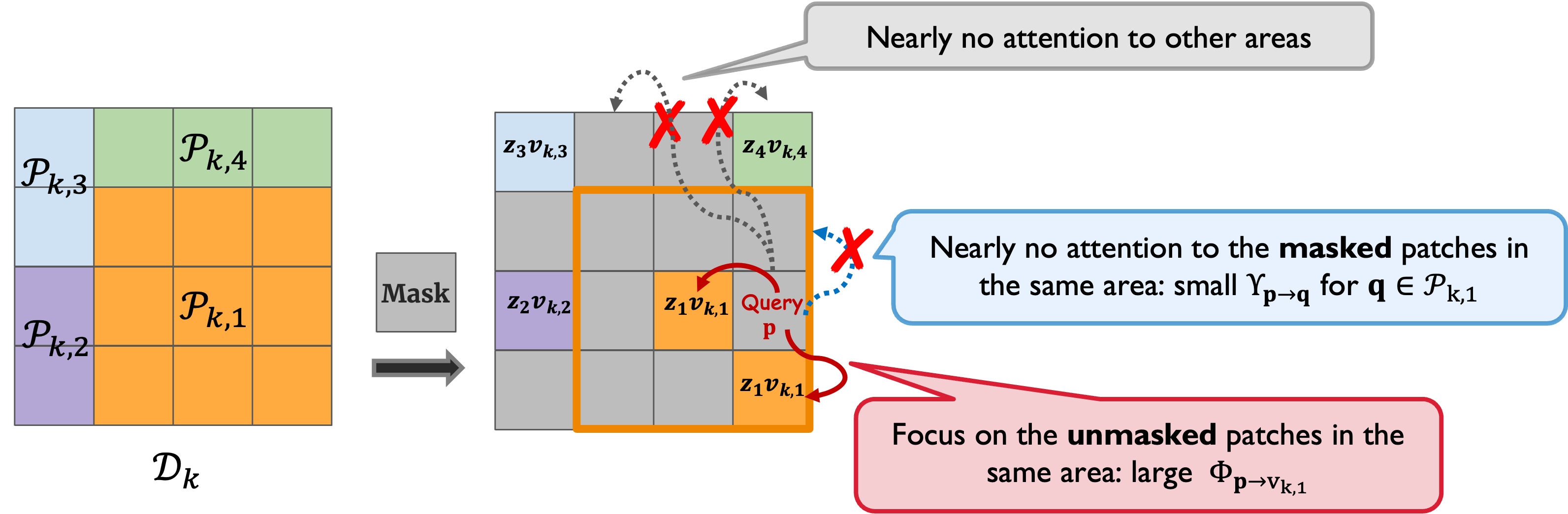
Figure 2: The mechanism of how the masked patch attends to other patches through attention correlations after MIM pretraining.

Area attention scores.

We first define a new notation for a cleaner presentation. Let $X\sim\mathcal{D}$. We choose a patch $\mathbf{p}\in\mathcal{P}$ and write the attention of patch $\mathbf{p}$ to a subset $\mathcal{A}\subset\mathcal{P}$ of patches by

$$\textstyle\widetilde{\mathbf{Attn}}_{{\mathbf{p}}\to\mathcal{A}}(X;Q)\coloneqq\sum_{\mathbf{q}\in\mathcal{A}}\mathbf{attn}_{\mathbf{p}\to\mathbf{q}}(X;Q).$$ (3.1)

We now explain why the above notion of area attention matters in understanding how attention works in masked reconstruction. Suppose now we have a sample $X\sim\mathcal{D}_{k}$ where patch $X_{\mathbf{p}}$ with $\mathbf{p}\in\mathcal{P}_{k,m}$ is masked, i.e., $\mathbf{p}\in\mathcal{M}$. Then the prediction of $X_{\mathbf{p}}$ given masked input $\mathsf{M}(X)$ can be written as

$$[F(\mathsf{M}(X);Q)]_{{\mathbf{p}}} \textstyle=\sum_{{\mathbf{q}}\in\mathcal{P}}\mathsf{M}(X)_{{\mathbf{q}}}\cdot\mathbf{attn}_{{\mathbf{p}}\to{\mathbf{q}}}(\mathsf{M}(X);Q)$$

$$\textstyle=\sum_{i\in[N_{k}]}z_{i}(X)v_{k,i}\cdot\widetilde{\mathbf{Attn}}_{{\mathbf{p}}\to\mathcal{U}\cap\mathcal{P}_{k,i}}(\mathsf{M}(X);Q). \mathsf{M}(X)_{\mathbf{q}}=\mathbf{0} \mathbf{q}\in\mathcal{M}$$ (because if )

Here we note that, to reconstruct the original patch $X_{\mathbf{p}}=z_{m}(X)v_{k,m}$, the transformer $F$ not only needs to identify and focus on the correct area $\mathcal{P}_{k,m}$ with the area attention score $\widetilde{\mathbf{Attn}}_{{\mathbf{p}}\to\mathcal{P}_{k,m}}$, where the same feature lies, but must also prioritize attention to the unmasked patches within this area. This specificity is denoted by the attention score $\widetilde{\mathbf{Attn}}_{{\mathbf{p}}\to\mathcal{U}\cap\mathcal{P}_{k,m}}$, a requirement imposed by masking operations. To further explain the differences between these two types of attention, we introduce the following definition, which is helpful in our proofs and captures the major novelty of our analysis that differentiates from those in [23].

Definition 3.1.

(Attention correlations) Let ${\mathbf{p}},{\mathbf{q}}\in\mathcal{P}$. We define two types of attention correlations as:

1. Feature-Position (FP) Correlation: $\Phi_{{\mathbf{p}}\to v_{k,m}}\coloneqq e^{\top}_{{\mathbf{p}}}Qv_{k,m},\ k\in[K]$ and $m\in[N_{k}]$;

2. Position-Position (PP) Correlation: $\Upsilon_{{\mathbf{p}}\to{\mathbf{q}}}\coloneqq e_{{\mathbf{p}}}^{\top}Qe_{{\mathbf{q}}},\ \forall\mathbf{p},\mathbf{q}\in\mathcal{P};$

Due to our (zero) initialization of $Q^{(0)}$, we have $\Phi^{(0)}_{{\mathbf{p}}\to{v_{k,m}}}=\Upsilon^{(0)}_{{\mathbf{p}}\to{\mathbf{q}}}=0$.

The importance of the FP correlation $\Phi$ and the PP correlation $\Upsilon$ defined above can be seen from how they determine the area attention scores as follows. Given a masked input $\mathsf{M}(X)$, for the attention of area $\mathcal{P}_{k,m}$, it holds that

$$\widetilde{\mathbf{Attn}}_{{\mathbf{p}}\to\mathcal{P}_{k,m}}(\mathsf{M}(X);Q)\propto\sum_{\mathbf{q}\in\mathcal{P}_{k,m}\cap\mathcal{U}}e^{\Phi_{\mathbf{p}\to v_{k,m}}+\Upsilon_{\mathbf{p}\to\mathbf{q}}}+\sum_{\mathbf{q}\in\mathcal{P}_{k,m}\cap\mathcal{M}}e^{\Upsilon_{\mathbf{p}\to\mathbf{q}}},$$ (3.2)

where the first term on the RHS is proportional to $\widetilde{\mathbf{Attn}}_{{\mathbf{p}}\to\mathcal{U}\cap\mathcal{P}_{k,m}}(\mathsf{M}(X);Q)$. Apparently, the attention scores are balanced by the relative magnitude between $\Phi_{\mathbf{p}\to v_{k,m}}$ and $\Upsilon_{\mathbf{p}\to\mathbf{q}}$, and it is easy to note that learning $\Phi_{\mathbf{p}\to v_{k,m}}$ would reach a lower final loss in the reconstruction objective (illustrated in Figure 2). Hence, understanding how the model trains and converges towards accurate image reconstruction can be achieved by examining how the attention mechanism evolves, especially how these two types of attention correlation changes during training. To present the results with simpler notations, we further define the unmasked area attention as follows:

$$\textstyle\mathbf{Attn}_{{\mathbf{p}}\to\mathcal{P}_{k,m}}(\mathsf{M}(X);Q)\coloneqq\widetilde{\mathbf{Attn}}_{{\mathbf{p}}\to\mathcal{U}\cap\mathcal{P}_{k,m}}(\mathsf{M}(X);Q),$$

and we also abbreviate $\mathbf{Attn}_{{\mathbf{p}}\to\mathcal{P}_{k,m}}(\mathsf{M}(X);Q^{(t)})$ and $\mathbf{attn}_{\mathbf{p}\to\mathbf{q}}(\mathsf{M}(X);Q^{(t)})$) as $\mathbf{Attn}_{{\mathbf{p}}\to\mathcal{P}_{k,m}}^{(t)}$ and $\mathbf{attn}_{\mathbf{p}\to\mathbf{q}}^{(t)}$.

3.1 Significance of the Feature-Position Correlation

The construction of attention correlation provides a framework where the transformer could attain a certain locality through learning the FP correlation, which is a meaningful generalization on top of prior works [23, 35]. Below we further discuss the significance of FP correlation by highlighting a notable gap in existing theoretical studies of transformers: a lack of characterization of the process in which different features in a multi-patch input are learned to be correctly associated by transformers. We point out important cases where the prior works were unable to address.

Can pure positional attention explain the transformer’s ability to learn locality?

[23] presented a theoretical explanation of how ViTs can identify spatially localized patterns by minimizing the supervised cross-entropy loss with gradient descent. Their analysis focused on a spatially structured dataset equivalent to our data settings when there is a single cluster ($K=1$), without distinguishing the global and local features. Due to their data assumption where patch-feature associations are invariant, the optimal attention mechanism can depend solely on the positional encodings. More specifically, the optimal attention from patch $X_{\mathbf{p}}$ to $X_{\mathbf{q}}$ can rely on only $e_{\mathbf{p}}^{\top}Q^{(t)}e_{\mathbf{q}}$ (the PP correlation in our setting). They show that ViTs can learn the so-called “patch association”, i.e. $e_{\mathbf{p}}^{\top}Q^{(t)}e_{\mathbf{q}}$ is large for $X_{\mathbf{q}}$ coming from the same area as $X_{\mathbf{p}}$, but the association is determined by the positions of patches in an absolute manner. Such an assumption of invariant patch associations is often unrealistic for vision datasets in practice, as different features like shapes and textures are usually of different spatial structures, which requires different patch association patterns to extract and aggregate. Clearly, a cube-shaped building requires a different attention pattern to a bird inside the woods. Therefore, when various patterns appear in the data distribution (e.g., in our settings with more than one cluster $K>1$), relying solely on positional correlations is insufficient. This highlights the necessity of examining feature-position correlations, which have considerable value in a more generalized setting, for a deeper understanding of the local representation power of transformers.

Can theories of MIM without positional encodings be enough to explain its power?

The theoretical work [35] analyzed the feature learning process of MIM pretraining with CNN architectures, without any patch-level positional structure in the network. The main implication of their theoretical result is that the trained CNNs provably already identify all discriminative features during MIM’s pretraining. However, leaving out ViTs which is the dominant architecture in MIM suggests a gap between theory and practice. Moreover, recent works have suggested that the adoption of transformers is not only for the convenience of engineering. Studies like [33, 53] reveal the distinct advantages of MIM through the lens of self-attention investigation, particularly its ability to learn diverse local patterns and avoid collapsing solutions. Such evidence suggests that the reason behind MIM’s success may fall beyond what CNN-based analysis could reveal, emphasizing the importance of studying attention patterns from a theoretical point of view.

4 Main Results

In this section, we present our main theoretical results on how transformers capture target feature-position (FP) correlations while downplaying position-wise correlations in the training process.

Information gap and a technical condition.

Based on our data model in Section 2.2, we further introduce a concept termed the information gap to quantify the difference of significance between the global and the local areas (cf. Assumption 2.2). Denoted as $\Delta$, the information gap is formally defined as follows:

$$\Delta\coloneqq(1-\kappa_{s})-2(1-\kappa_{c}).$$ (4.1)

Our study focuses on the regime, where $\Delta$ is not too close to zero, i.e. $|\Delta|=\Omega(1)$, which allows for cleaner induction arguments. This condition could be potentially relaxed via more involved analysis.

Notations for theorem and proof presentations.

Firstly, any variable with superscript ^(t) refers to the corresponding variable at the $t$-th step of the training process. We use $k_{X}\in[K]$ to denote the cluster index that a given image $X$ is drawn from. We use $a_{k,\mathbf{p}}$ to indicate that the index of the area $\mathbf{p}$ is located in the cluster $\mathcal{D}_{k}$, i.e., $\mathbf{p}\in\mathcal{P}_{k,a_{k,\mathbf{p}}}$. We further use $\mathcal{C}_{\mathbf{p}}\coloneqq\{k\in[K]:\mathbf{p}\in\mathcal{P}_{k,1}\}$ and $\mathcal{B}_{\mathbf{p}}\coloneqq[K]\setminus\mathcal{C}_{\mathbf{p}}$ to denote the clusters into which ${\mathbf{p}}$ falls in the global and local areas, respectively. To properly evaluate the reconstructing performance, we further introduce the following notion of the reconstruction loss with respect to a specific patch $\mathbf{p}\in\mathcal{P}$:

$$\mathcal{L}_{\mathbf{p}}(Q) =\frac{1}{2}\mathbb{E}\left[\operatorname{\mathds{1}}\{{\mathbf{p}}\in\mathcal{M}\}\Big{\|}[F(\mathsf{M}(X);Q)]_{{\mathbf{p}}}-X_{{\mathbf{p}}}\Big{\|}^{2}\right].$$ (4.2)

Now we present our main theorem, which characterizes the global convergence of the loss function and the attention pattern at the time of convergence.

Theorem 4.1.

Suppose the information gap $\Delta\in[-0.5,-\Omega(1)]\cup[\Omega(1),1]$. For any $0<\epsilon<1$, suppose $\operatorname{polylog}(P)\gg\log(\frac{1}{\epsilon})$. We apply GD to train the MIM loss function given in (2.8) with $\eta\ll\operatorname{poly}(P)$. Then for each patch $\mathbf{p}\in\mathcal{P}$, we have

1. $\mathcal{L}_{\mathbf{p}}(Q^{(T^{\star})})-\mathcal{L}_{\mathbf{p}}^{\star}\leq\epsilon$ in

   $$T^{\star}=O\Big{(}\frac{1}{\eta}\log(P)P^{\max\{2(\frac{U}{L}-1),1\}(1-\kappa_{s})}+\frac{1}{\eta\epsilon}\log\big{(}\frac{P}{\epsilon}\big{)}\Big{)}$$

   iterations, where ${\mathcal{L}}_{\mathbf{p}}^{\star}$ is the global minimum of patch-level reconstruction loss in (4.2).

2. Area-wide pattern of attention: given cluster $k\in[K]$, if $X_{\mathbf{p}}$ is masked, then the one-layer transformer nearly “pays all attention” to all unmasked patches in the same area $\mathcal{P}_{k,a_{k,\mathbf{p}}}$, i.e.,

   $$\Big{(}1-\mathbf{Attn}_{{\mathbf{p}}\to\mathcal{P}_{k,a_{k,\mathbf{p}}}}^{(T^{\star})}\Big{)}^{2}\leq O(\epsilon).$$

Theorem 4.1 indicates that, at the end of the training, for any masked query patch $X_{\mathbf{p}}$ in the $k$-th cluster, the transformer exhibits an area-wide pattern of attention, concentrating on those unmasked patches within the area $\mathcal{P}_{k,a_{k,\mathbf{p}}}$, i.e., the area in which $X_{\mathbf{p}}$ is located.

Implications of the theorem.

The area-wide pattern of attention at the end of training suggests that regardless of whether a patch $\mathbf{p}$ belongs to a global or a local area, the FP correlation $\Phi_{{\mathbf{p}}\to v_{k,a_{k,\mathbf{p}}}}$ will be learned. As we discuss in Section 3, a high position-wise correlation $\Upsilon_{{\mathbf{p}}\to{\mathbf{q}}}$ for $\mathbf{q}\in\mathcal{P}_{k,a_{k,\mathbf{p}}}$, may also contribute to increased attention towards the area $\mathcal{P}_{k,a_{k,\mathbf{p}}}$, which mirrors the concept “patch association” in [23], wherein the attention is solely determined by positional encoding. However, two key issues can arise: i) such position association varies for different clusters, i.e., $a_{k,\mathbf{p}}=a_{k,\mathbf{q}}$, which does not necessarily hold for all $k\in[K]$; ii) such mechanism may also inadvertently direct attention towards the undesired masked patches, which leads to a flawed optimization of $\mathbf{Attn}^{(t)}_{\mathbf{p}\to\mathcal{P}_{k,a_{k,\mathbf{p}}}}$. Consequently, the analysis in [23] cannot be applied to the settings where data exhibit varying spatial structures, such as distinct feature-area associations in our setting. Our characterization for the learning dynamics of MIM in Section 5 verifies this implication and explicitly demonstrates that the target FP correlation will be learned eventually and all PP correlations remain negligible.

Note that our proof of Theorem 4.1 will differ between $\Delta$ under positive and negative conditions (although they are presented in a unified way in Theorem 4.1), as the learning process for local areas exhibits distinct dynamic behaviors under those two conditions.

5 Overview of the Proof Techniques

In this section, we explain our key proof techniques in analyzing the MIM pretraining of transformers. We focus on the reconstruction of a specific patch $X_{\mathbf{p}}$ for $\mathbf{p}\in\mathcal{P}$. We aim to elucidate the training phases through which the model learns FP correlations related to the area associated with $\mathbf{p}$ across different clusters $k\in[K]$.

Our characterization of training phases differentiates between whether $X_{\mathbf{p}}$ is located in the global or local areas and further varies based on whether $\Delta$ is positive or negative. Specifically, for $\Delta\in[\Omega(1),1]$, we observe distinct learning dynamics for FP correlations between local and global areas:

• Local area attends to FP correlation in two-phase: given $k\in[K]$, if $a_{k,\mathbf{p}}\neq 1$, then

  1. $\Phi^{(t)}_{\mathbf{p}\to v_{k,1}}$ first quickly decreases whereas all other $\Phi^{(t)}_{\mathbf{p}\to v_{k,m}}$ with $m\not=1$ and $\Upsilon^{(t)}_{\mathbf{p}\to\mathbf{q}}$ do not change much;

  2. after some point, the increase of $\Phi^{(t)}_{\mathbf{p}\to v_{k,a_{k,\mathbf{p}}}}$ takes dominance. Such $\Phi^{(t)}_{\mathbf{p}\to v_{k,a_{k,\mathbf{p}}}}$ will keep growing until convergence with all other FP and PP attention correlations nearly unchanged.

• Global areas learn FP correlation in one-phase: given $k\in[K]$, if $a_{k,\mathbf{p}}=1$, the update of $\Phi^{(t)}_{\mathbf{p}\to v_{k,1}}$ will dominate throughout the training, whereas all other $\Phi^{(t)}_{\mathbf{p}\to v_{k,m}}$ with $m\not=1$ and learned PP correlations remain close to $0$.

For $\Delta\in[-0.5,-\Omega(1)]$, the behaviors of learning FP correlations are uniform for all areas. Namely, all areas learn FP correlation through one-phase: given $k\in[K]$, throughout the training, the increase of $\Phi^{(t)}_{\mathbf{p}\to v_{k,a_{k,\bm{p}}}}$ dominates, whereas all other $\Phi^{(t)}_{\mathbf{p}\to v_{k,m}}$ with $m\not=a_{k,\mathbf{p}}$ and PP correlations $\Upsilon^{(t)}_{\mathbf{p}\to\mathbf{q}}$ remain close to $0$.

For clarity, this section will mainly focus on the learning of local feature correlations with a positive information gap $\Delta\geq\Omega(1)$ in Sections 5.2 and 5.3, which exhibits a two-phase process. The other scenarios will be discussed briefly in Section 5.4.

5.1 GD Dynamics of Attention Correlations

Based on the crucial roles that attention correlations play in determining the reconstruction loss, the main idea of our analysis is to track the dynamics of those attention correlations. We first provide the following GD updates of $\Phi^{(t)}_{{\mathbf{p}}\to v_{k,m}}$ and $\Upsilon_{\mathbf{p}\to\mathbf{q}}^{(t)}$ (see Appendix A.1.1 for formal statements).

Lemma 5.1 (FP correlations, informal).

Given $k\in[K]$, for ${\mathbf{p}}\in\mathcal{P}$, denote $n=a_{k,\mathbf{p}}$, let $\alpha^{(t)}_{{\mathbf{p}}\to{v_{k,m}}}=\frac{1}{\eta}\big{(}\Phi^{(t+1)}_{{\mathbf{p}}\to v_{k,m}}-\Phi^{(t)}_{{\mathbf{p}}\to v_{k,m}}\big{)}$ for $m\in[N_{k}]$, and suppose $X_{\mathbf{p}}$ is masked. Then

1. for the same area, $\alpha^{(t)}_{{\mathbf{p}}\to{v_{k,n}}}\approx\mathbf{Attn}^{(t)}_{{\mathbf{p}}\to\mathcal{P}_{k,n}}\left(1-\mathbf{Attn}^{(t)}_{{\mathbf{p}}\to\mathcal{P}_{k,n}}\right)^{2};$

2. if $k\in\mathcal{B}_{\mathbf{p}}$, for the global area,

   $$\alpha^{(t)}_{{\mathbf{p}}\to{v_{k,1}}} \approx-\mathbf{Attn}^{(t)}_{{\mathbf{p}}\to\mathcal{P}_{k,1}}\cdot\Bigg{(}\mathbf{Attn}^{(t)}_{{\mathbf{p}}\to\mathcal{P}_{k,1}}\left(1-\mathbf{Attn}^{(t)}_{{\mathbf{p}}\to\mathcal{P}_{k,1}}\right)+\mathbf{Attn}^{(t)}_{{\mathbf{p}}\to\mathcal{P}_{k,n}}\left(1-\mathbf{Attn}^{(t)}_{{\mathbf{p}}\to\mathcal{P}_{k,n}}\right)\Bigg{)};$$

3. for other area $m\notin\{n\}\cup\{1\}$,

   $$\alpha^{(t)}_{{\mathbf{p}}\to{v_{k,m}}}\approx\mathbf{Attn}^{(t)}_{{\mathbf{p}}\to\mathcal{P}_{k,m}}\Bigg{(}\operatorname{\mathds{1}}{\{n\not=1\}}\left(\mathbf{Attn}^{(t)}_{{\mathbf{p}}\to\mathcal{P}_{k,1}}\right)^{2}-\left(1-\mathbf{Attn}^{(t)}_{{\mathbf{p}}\to\mathcal{P}_{k,n}}\right)\mathbf{Attn}^{(t)}_{{\mathbf{p}}\to\mathcal{P}_{k,n}}\Bigg{)}.$$

From Lemma 5.1, it is observed that for ${\mathbf{p}}\in\mathcal{P}_{k,n}$, the feature correlation $\Phi^{(t)}_{{\mathbf{p}}\to v_{k,n}}$ exhibits a monotonically increasing trend over time because $\alpha_{{\mathbf{p}}\to v_{k,n}}^{(t)}\geq 0$. Furthermore, if $n>1$, i.e., $\mathcal{P}_{k,n}$ is the local area, $\Phi^{(t)}_{{\mathbf{p}}\to v_{k,1}}$ will monotonically decrease.

Lemma 5.2 (PP attention correlations, informal).

Given ${\mathbf{p}},{\mathbf{q}}\in\mathcal{P}$, let $\beta^{(t)}_{{\mathbf{p}}\to{\mathbf{q}}}=\frac{1}{\eta}\big{(}\Upsilon^{(t+1)}_{{\mathbf{p}}\to{\mathbf{q}}}-\Upsilon^{(t)}_{{\mathbf{p}}\to{\mathbf{q}}}\big{)}$, and suppose $X_{\mathbf{p}}$ is masked. Then $\beta^{(t)}_{{\mathbf{p}}\to{\mathbf{q}}}=\sum_{k\in[N]}\beta^{(t)}_{k,{\mathbf{p}}\to{\mathbf{q}}}$, where $\beta^{(t)}_{k,{\mathbf{p}}\to{\mathbf{q}}}$ satisfies

1. if $a_{k,\mathbf{p}}=a_{k,\mathbf{q}}=n$, $\beta^{(t)}_{k,{\mathbf{p}}\to{\mathbf{q}}}\approx\mathbf{attn}^{(t)}_{{\mathbf{p}}\to{\mathbf{q}}}\left(1-\mathbf{Attn}^{(t)}_{{\mathbf{p}}\to\mathcal{P}_{k,n}}\right)^{2};$

2. if $k\in\mathcal{B}_{\mathbf{p}}\cap\mathcal{C}_{\mathbf{q}}$, where $a_{k,\mathbf{p}}=n>1$ and $a_{k,\mathbf{q}}=1$:

   $$\beta^{(t)}_{k,{\mathbf{p}}\to{\mathbf{q}}} \approx-\mathbf{attn}^{(t)}_{{\mathbf{p}}\to\mathbf{q}}\cdot\Bigg{(}\mathbf{Attn}^{(t)}_{{\mathbf{p}}\to\mathcal{P}_{k,1}}\left(1-\mathbf{Attn}^{(t)}_{{\mathbf{p}}\to\mathcal{P}_{k,1}}\right)+\mathbf{Attn}^{(t)}_{{\mathbf{p}}\to\mathcal{P}_{k,n}}\left(1-\mathbf{Attn}^{(t)}_{{\mathbf{p}}\to\mathcal{P}_{k,n}}\right)\Bigg{)};$$

3. if $a_{k,\mathbf{q}}=m\notin\{n\}\cup\{1\}$, where $a_{k,\mathbf{p}}=n$,

   $$\beta^{(t)}_{k,{\mathbf{p}}\to\mathbf{q}}\approx\mathbf{attn}^{(t)}_{{\mathbf{p}}\to\mathbf{q}}\cdot\Bigg{(}\operatorname{\mathds{1}}{\{n\not=1\}}\left(\mathbf{Attn}^{(t)}_{{\mathbf{p}}\to\mathcal{P}_{k,1}}\right)^{2}-\left(1-\mathbf{Attn}^{(t)}_{{\mathbf{p}}\to\mathcal{P}_{k,n}}\right)\mathbf{Attn}^{(t)}_{{\mathbf{p}}\to\mathcal{P}_{k,n}}\Bigg{)}.$$

Based on the above gradient update for $\Upsilon^{(t)}_{\mathbf{p}\to\mathbf{q}}$, we further introduce the following auxiliary quantity $\Upsilon^{(t)}_{k,\mathbf{p}\to\mathbf{q}}$, which can be interpreted as the PP attention correlation “projected” on the $k$-th cluster $\mathcal{D}_{k}$, and will be useful in the later proof.

$$\Upsilon^{(t+1)}_{k,\mathbf{p}\to\mathbf{q}}\coloneqq\Upsilon^{(t)}_{k,\mathbf{p}\to\mathbf{q}}+\eta\beta^{(t)}_{k,\mathbf{p}\to\mathbf{q}},\quad\text{ with }\Upsilon^{(0)}_{k,\mathbf{p}\to\mathbf{q}}=0.$$ (5.1)

We can directly verify that $\Upsilon^{(t)}_{\mathbf{p}\to\mathbf{q}}=\sum_{k\in[K]}\Upsilon^{(t)}_{k,\mathbf{p}\to\mathbf{q}}$.

The key observation by comparing Lemma 5.1 and 5.2 is that the gradient of projected PP attention $\beta^{(t)}_{k,{\mathbf{p}}\to\mathbf{q}}$ is smaller than the corresponding FP gradient $\alpha_{\mathbf{p}\to v_{k,a_{k,\mathbf{q}}}}^{(t)}$ in magnitude since $\textstyle\mathbf{attn}^{(t)}_{{\mathbf{p}}\to\mathbf{q}}\approx\frac{\mathbf{Attn}^{(t)}_{{\mathbf{p}}\to\mathcal{P}_{k,a_{k,\mathbf{q}}}}}{(1-\gamma)C_{k,a_{k,\mathbf{q}}}}$. We will show that the interplay between the increase of $\Phi^{(t)}_{{\mathbf{p}}\to v_{k,n}}$ and the decrease of $\Phi^{(t)}_{{\mathbf{p}}\to v_{k,1}}$ determines the learning behaviors for the local patch $\mathbf{p}\in\mathcal{P}_{k,n}$ with $n>1$, and which effect will happen first depends on the initial attention, which is also determined by the value of information gap $\Delta$.

5.2 Phase I: Decoupling the Global FP Correlations

We now explain how the attention correlations evolve at the initial phase of the training to decouple the correlations of the non-target global features when $\mathbf{p}$ is located in the local area for the $k$-th cluster. This phase can be further divided into the following two stages.

Stage 1.

At the beginning of training, $\Phi^{(0)}_{\mathbf{p}\to v_{k,m}}=\Upsilon^{(0)}_{k,\mathbf{p}\to\mathbf{q}}=0$, and hence $\mathbf{attn}^{(0)}_{\mathbf{p}\to{\mathbf{q}}}=\frac{1}{P}$ for any ${\mathbf{q}}\in\mathcal{P}$, which implies that the transformer equally attends to each patch. However, with high probability, the number of unmasked global features in the global area $\mathcal{P}_{k,1}$ is much larger than others. Hence, $\mathbf{Attn}_{\mathbf{p}\to\mathcal{P}_{k,1}}^{(0)}=\frac{|\mathcal{U}\cap\mathcal{P}_{k,1}|}{P}\geq\Omega(\frac{1}{P^{1-\kappa_{c}}})\gg\Theta(\frac{1}{P^{1-\kappa_{s}}})=\mathbf{Attn}_{\mathbf{p}\to\mathcal{P}_{k,m}}^{(0)}$ for $m>1$. Therefore, by Lemma 5.1 and 5.2, we immediately obtain

• $\alpha_{\mathbf{p}\to v_{k,1}}^{(0)}=-\Theta\Big{(}\frac{1}{P^{2(1-\kappa_{c})}}\Big{)}$, whereas $\alpha_{\mathbf{p}\to v_{k,a_{k,\mathbf{p}}}}^{(0)}=\Theta\Big{(}\frac{1}{P^{(1-\kappa_{s})}}\Big{)}$;

• all other FP correlation gradients $\alpha_{\mathbf{p}\to v_{k,m}}^{(0)}$ with $m\not=1,a_{k,\mathbf{p}}$ are small;

• all projected PP correlation gradients $\beta^{(0)}_{k,\mathbf{p}\to\mathbf{q}}$ are small.

Since $\Delta=(1-\kappa_{s})-2(1-\kappa_{c})\geq\Omega(1)$, it can be seen that $\Phi_{\mathbf{p}\to v_{k,1}}^{(t)}$ enjoys a much larger decreasing rate initially. This captures the decoupling process of the feature correlations with the global feature $v_{k,1}$ in the global area for $\mathbf{p}$. It can be shown that such an effect will dominate over a certain period that defines stage 1 of phase I. At the end of this stage, we will have $\Phi_{\mathbf{p}\to v_{k,1}}^{(t)}\leq-\Omega\left(\log(P)\right)$, whereas all FP attention correlation $\Phi_{\mathbf{p}\to v_{k,m}}^{(t)}$ with $m>1$ and all projected PP correlations $\Upsilon_{k,\mathbf{p}\to\mathbf{q}}^{(t)}$ stay close to $0$ (see Section C.1).

During stage 1, the significant decrease of the global FP correlation $\Phi_{\mathbf{p}\to v_{k,1}}^{(t)}$ leads to a reduction in the attention score $\mathbf{Attn}_{\mathbf{p}\to\mathcal{P}_{k,1}}^{(t)}$. Meanwhile, attention scores $\mathbf{Attn}^{(t)}_{\mathbf{p}\to\mathcal{P}_{k,m}}$ (where $m>1$) for other patches remain consistent, reflecting a uniform distribution over unmasked patches within each area. By the end of stage 1, $\mathbf{Attn}_{\mathbf{p}\to\mathcal{P}_{k,1}}^{(t)}$ drops to a certain level, resulting in a decrease in $|\alpha_{\mathbf{p}\to v_{k,1}}^{(t)}|$ as it approaches $\alpha_{\mathbf{p}\to v_{k,n}}^{(t)}$, which indicates that stage 2 begins.

Stage 2.

Soon as stage 2 begins, the dominant effect switches as $|\alpha^{(t)}_{\mathbf{p}\to v_{k,1}}|$ reaches the same order of magnitude as $\alpha_{\mathbf{p}\to v_{k,a_{k,\mathbf{p}}}}^{(t)}$. The following result shows that $\Phi_{\mathbf{p}\to v_{k,a_{k,\mathbf{p}}}}^{(t)}$ must update during stage 2.

Lemma 5.3 (Switching of dominant effects (See Section C.2)).

Under the same conditions as Theorem 4.1, for $\mathbf{p}\in\mathcal{P}$, there exists $\widetilde{T}_{1}$, such that at iteration $t=\widetilde{T}_{1}+1$, we have

1. $\Phi_{\mathbf{p}\to v_{k,a_{k,\mathbf{p}}}}^{(\widetilde{T}_{1}+1)}\geq\Omega\left(\log(P)\right)$, and $\Phi_{\mathbf{p}\to v_{k,1}}^{(\widetilde{T}_{1}+1)}=-\Theta(\log(P))$;

2. all other FP correlations $\Phi_{\mathbf{p}\to v_{k,m}}^{(t)}$ with $m\not=1,a_{k,\mathbf{p}}$ are small;

3. all projected PP correlations $\Upsilon^{(t)}_{k,\mathbf{p}\to\mathbf{q}}$ are small.

Intuition of the transition.

Once $\Phi_{\mathbf{p}\to v_{k,1}}^{(t)}$ decreases to $-\frac{\Delta}{2L}\log(P)$, we observe that $|\alpha_{\mathbf{p}\to v_{k,1}}^{(t)}|$ is approximately equal to $\alpha_{\mathbf{p}\to v_{k,a_{k,\mathbf{p}}}}^{(t)}$. After this point, reducing $\Phi_{\mathbf{p}\to v_{k,1}}^{(t)}$ further is more challenging compared to the increase in $\Phi_{\mathbf{p}\to v_{k,a_{k,\mathbf{p}}}}^{(t)}$. To illustrate, a minimal decrease of $\Phi_{\mathbf{p}\to v_{k,1}}^{(t)}$ by an amount of $\frac{0.001}{L}\log(P)$ will yield $|\alpha_{\mathbf{p}\to v_{k,1}}^{(t)}|\leq O(\frac{\alpha_{\mathbf{p}\to v_{k,n}}^{(t)}}{P^{0.002}})$. Such a discrepancy triggers the switch of the dominant effect.

5.3 Phase II: Growth of Target Local FP Correlation

Moving beyond phase I, FP correlation $\Phi_{\mathbf{p}\to v_{k,a_{k,\mathbf{p}}}}^{(t)}$ within the target local area $\mathbf{p}$ already enjoys a larger gradient $\alpha_{\mathbf{p}\to v_{k,a_{k,\mathbf{p}}}}^{(t)}$ than other $\Phi_{\mathbf{p}\to v_{k,m}}^{(t)}$ with $m\not=a_{k,\mathbf{p}}$ and all projected PP correlations $\Upsilon_{k,\mathbf{p}\to\mathbf{q}}^{(t)}$. We can show that the growth of $\Phi_{\mathbf{p}\to v_{k,a_{k,\mathbf{p}}}}^{(t)}$ will continue to dominate until the end of training by recognizing the following two stages.

Rapid growth stage.

At the beginning of phase II, $\alpha_{\mathbf{p}\to v_{k,a_{k,\mathbf{p}}}}^{(t)}$ is mainly driven by $\mathbf{Attn}_{\mathbf{p}\to\mathcal{P}_{k,a_{k,\mathbf{p}}}}^{(t)}$ since $1-\mathbf{Attn}_{\mathbf{p}\to\mathcal{P}_{k,a_{k,\mathbf{p}}}}^{(t)}$ remains at the constant order. Therefore, the growth of $\Phi_{\mathbf{p}\to v_{k,a_{k,\mathbf{p}}}}^{(t)}$ naturally results in a boost in $\mathbf{Attn}_{\mathbf{p}\to\mathcal{P}_{k,a_{k,\mathbf{p}}}}^{(t)}$, thereby promoting an increase in its own gradient $\alpha_{\mathbf{p}\to v_{k,a_{k,\mathbf{p}}}}^{(t)}$, which defines the rapid growth stage. On the other hand, we can prove that the following gap holds for FP and projected PP correlation gradients (see Section C.3):

• all other FP correlation gradients $\alpha_{\mathbf{p}\to v_{k,m}}^{(t)}$ with $m\not=a_{k,\mathbf{p}}$ are small;

• all projected PP correlation gradients $\beta^{(t)}_{k,\mathbf{p}\to\mathbf{q}}$ are small.

Convergence stage.

After the rapid growth stage, the desired local pattern with a high target feature-position correlation $\Phi_{\mathbf{p}\to v_{k,a_{k,\mathbf{p}}}}^{(t)}$ is learned. In this last stage, it is demonstrated that the above conditions for non-target FP and projected PP correlations remain valid, while the growth of $\Phi_{\mathbf{p}\to v_{k,a_{k,\mathbf{p}}}}^{(t)}$ starts to decelerate as $\Phi_{\mathbf{p}\to v_{k,a_{k,\mathbf{p}}}}^{(t)}$ reaches $\Theta(\log(P))$, resulting in $\mathbf{Attn}_{\mathbf{p}\to\mathcal{P}_{k,n}}^{(t)}\approx\Omega(1)$, which leads to convergence (see Section C.4).

5.4 Learning Processes in Other Scenarios

In this section, we talk about the learning process in other settings, including learning FP correlations for the local area when the information gap is negative, learning FP correlations for the global area, and failure to learn PP correlations.

What is the role of positive information gap?

As described in stage 1 of phase 1 in Section 5.2, the decoupling effect happens at the beginning of the training because $\alpha_{\mathbf{p}\to v_{k,1}}^{(0)}\gg\alpha_{\mathbf{p}\to v_{k,a_{k,\mathbf{p}}}}^{(0)}$ attributed to $\Delta\geq\Omega(1)$. However, in cases where $\Delta\leq-\Omega(1)$, this relationship reverses, with $\alpha_{\mathbf{p}\to v_{k,1}}^{(0)}$ becoming significantly smaller than $\alpha_{\mathbf{p}\to v_{k,a_{k,\mathbf{p}}}}^{(0)}$. Similarly, other FP gradients $\alpha_{\mathbf{p}\to v_{k,m}}^{(0)}$ with $m\not=1,a_{k,\mathbf{p}}$ and all the projected gradients of PP correlation $\beta_{\mathbf{p}\to\mathbf{q}}^{(0)}$ are small in magnitude. Consequently, $\Phi_{\mathbf{p}\to v_{k,a_{k,\mathbf{p}}}}^{(t)}$ starts with a larger gradient, eliminating the need to decouple FP correlations for the global area. As a result, training skips the initial phase, and moves directly into Phase II, during which $\Phi_{\mathbf{p}\to v_{k,a_{k,\mathbf{p}}}}^{(t)}$ continues to increase until it converges (see Appendix D).

Learning FP correlations for the global area.

When the patch $X_{\mathbf{p}}$ is located in the global area of cluster $k$, i.e., $a_{k,\mathbf{p}}=1$, the attention score $\mathbf{Attn}^{(0)}_{\mathbf{p}\to\mathcal{P}_{k,1}}$ directed towards the target area $\mathcal{P}_{k,1}$ is initially higher compared to other attention scores due to the presence of a significant number of unmasked patches in the global area. This leads to an initially larger gradient $\alpha_{\mathbf{p}\to v_{k,a_{k,\mathbf{p}}}}^{(0)}$. Such an effect is independent of the value of $\Delta$. As a result, the training process skips the initial phase, which is typically necessary for the cases where $a_{k,\mathbf{p}}>1$ with a positive information gap, and moves directly into Phase II (see Appendix E).

All PP correlations are small.

Integrating the analysis from all previous discussions, we establish that for every cluster $k\in[K]$, regardless of its association with $\mathcal{C}_{\mathbf{p}}$ (global area) or $\mathcal{B}_{\mathbf{p}}$ (local area), and for any patch $X_{\mathbf{q}}$ with $\mathbf{q}\in\mathcal{P}$, the projected PP correlation $\Upsilon_{k,\mathbf{p}\to\mathbf{q}}^{(t)}$ remains nearly zero in comparison to the significant changes observed in the FP correlation, because the gradient $\beta_{k,\mathbf{p}\to\mathbf{q}}^{(t)}$ is relatively negligible. Therefore, the overall PP correlation $\Upsilon_{\mathbf{p}\to\mathbf{q}}^{(t)}=\sum_{k=1}^{K}\Upsilon_{k,\mathbf{p}\to\mathbf{q}}^{(t)}$ also stays close to zero, given that the number of clusters $K=\Theta(1)$.

6 Experiments

Previous studies on the attention mechanisms of ViT-based pre-training approaches have mainly utilized a metric known as the attention distance [11]. Such a metric quantifies the average spatial distance between the query and key tokens, weighted by their self-attention coefficients. The general interpretation is that larger attention distances indicate global understanding, and smaller values suggest a focus on local features. However, such a metric does not adequately determine if the self-attention mechanism is identifying a unique global pattern. A high attention distance could result from different patches focusing on varied distant areas, which does not necessarily imply that global information is being effectively synthesized. To address this limitation, we introduce a novel and revised version of average attention distance, called attention diversity metric, which is designed to assess whether various patches are concentrating on a similar region, thereby directly capturing global information.

Attention diversity metric, in distance.

This metric is computed for self-attention with a single head of the specific layer. For a given image divided into $P\times P$ patches, the process unfolds as follows: for each patch, it is employed as the query patch to calculate the attention weights towards all $P^{2}$ patches, and those with the top-$n$ attention weights are selected. Subsequently, the coordinates (e.g. $(i,j)$ with $i,j\in[P]$) of these top-$n$ patches are concatenated in sequence to form a $2\times n$-dimensional vector. The final step computes the average distance between all these $2n$-dimensional vectors, i.e., $P^{2}\times P^{2}$ vector pairs.

Setup.

In this work, we compare the performance of ViT-B/16 encoder pre-trained on ImageNet-1K [36] among the following four models: MIM model (MAE), contrastive learning model (MoCo v3 [10]), other self-supervised model (DINO [8]), and supervised model (DeiT [42]). We focus on $12$ different attention heads in the last layer of ViT-B on different pre-trained models. The box plot visualizes the distribution of the top-10 averaged attention focus across 152 example images, as similarly done in [11].

Implications.

The experiment results based on our new metric are provided in Figure 3. Lower values of the attention diversity metric signify a focused attention on a coherent area across different patches, reflecting a global pattern of focus. On the other hand, higher values suggest that attention is dispersed, focusing on different, localized areas. It can be seen that the MIM model is particularly effective in learning more diverse attention patterns, setting it apart from other models that prioritize a uniform global information with less attention diversity. This aligns with and provides further evidence for the findings in [33].

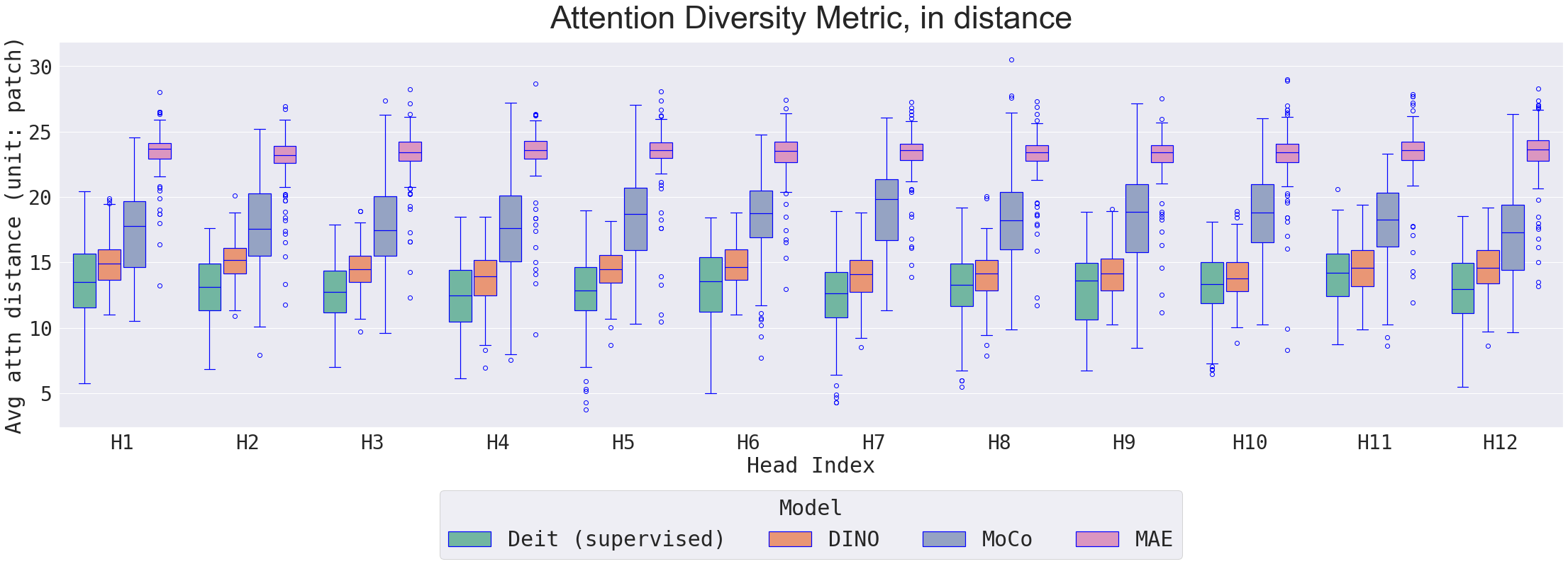
Figure 3: Attention Diversity Metric: We examined the last layer of ViT trained by MIM (MAE), contrastive learning (MoCo v3), non-contrastive learning (DINO), and supervised learning (DeiT). The results show that the MIM model excels in capturing diverse feature-position correlations. This capability leads to a strong focus on locality, distinguishing it from other models that emphasize uniform global information and exhibit less attention diversity.

7 Additional Related Work

Empirical studies of transformers in vision.

A number of works have aimed to understand the transformers in vision from different perspectives: comparison with CNNs [39, 14, 32], robustness [4, 31], and role of positional embeddings [29, 44]. Recent studies [57, 53, 33] have delved into ViTs with self-supervision to uncover the mechanisms at play, particularly through visualization and analysis of metrics related to self-attention. [57] compared the MIM’s method with supervised models, revealing MIM’s capacity to enhance diversity and locality across all ViT layers, w which significantly boosts performance on tasks with weak semantics following fine-tuning. Building on MIM’s advantages, [53] further proposed a simple feature distillation method that incorporates locality into various self-supervised methods, leading to an overall improvement in the finetuning performance. [33] conducted a detailed comparison between MIM and contrastive learning. They demonstrated that contrastive learning will make the self-attentions collapse into homogeneity for all query patches due to the nature of discriminative learning, while MIM leads to a diverse self-attention map since it focuses on local patterns.

Theory of self-supervised learning.

A major line of theoretical studies falls into one of the most successful self-supervised learning approaches, contrastive learning [54, 38, 7, 2], and its variant non-contrastive self-supervised learning [55, 34, 50]. Some other works study the mask prediction approach [25, 56, 24], which is the focus of this paper. [25] provided statistical downstream guarantees for reconstructing missing patches. [56] studied the benefits of head and prompt tuning with MIM pretraining under a Hidden Markov Model framework. [24] provided a parameter identifiability view to understand the benefit of masked prediction tasks, which linked the masked reconstruction tasks to the informativeness of the representation via identifiability techniques from tensor decomposition.

Theory of transformers and attention models.

Prior work has studied the theoretical properties of transformers from various aspects: representational power [59, 13, 47, 51, 40], internal mechanism [45, 52], limitations [18, 41], and PAC learning [6]. Recently, there has been a growing body of research studying in-context learning with transformers due to the remarkable emergent in-context ability of large language models [63, 48, 15, 1, 60, 19, 30, 26]. Regarding the training dynamics of attention-based models, [27] studied the training process of shallow ViTs in a classification task. Subsequent research expanded on this by exploring the graph transformer with positional encoding [28] and in-context learning performance of transformers with nonlinear self-attention and nonlinear MLP [26]. However, all of these analyses rely crucially on stringent assumptions on the initialization of transformers and hardly generalize to our setting. [46] mathematically described how the attention map evolves trained by SGD but did not provide any convergence guarantee. Furthermore, [19] proved the in-context convergence of a one-layer softmax transformer trained via GD and illustrated the attention dynamics throughout the training process. More recently, [30] studied GD dynamics on a simplified two-layer attention-only transformer and proved that it can encode the causal structure in the first attention layer. However, none of the previous studies analyzed the training of transformers under self-supervised learning, which is the focus of this paper.

8 Conclusion

In this work, we study the feature learning process of MIM with a one-layer softmax-based transformer. Our key contribution lies in showing that transformers trained with MIM exhibit local and diverse patterns by learning FP correlations. To our knowledge, our work is the first in analyzing softmax-based self-attention with both patch and position embedding simultaneously. Our proof techniques feature novel ideas for phase decomposition based on the interplay between feature-position and position-wise correlations, which do not need to disentangle patches and positional encodings as in prior works. We anticipate that our theory can be useful for future studies of the spatial structures inside transformers and can promote theoretical studies relevant to deep learning practice.

Appendix: The Proofs

Appendix A Preliminaries

In this section, we will introduce warm-up gradient computations and probabilistic lemmas that establish essential properties of the data and the loss function, which are pivotal for the technical proofs in the upcoming sections. Throughout the appendix, we assume $N_{k}=N$ and $C_{k,n}=C_{n}$ for all $k\in[K]$ for simplicity. We will also omit the explicit dependence on $X$ for $z_{n}(X)$.

A.1 Gradient Computations

We first calculate the gradient with respect to $Q$. We omit the superscript ‘$(t)$’ and write $\mathcal{L}(Q)$ as $\mathcal{L}$ here for simplicity.

Lemma A.1.

The gradient of the loss function with respect to $Q$ is given by

$$\frac{\partial\mathcal{L}}{\partial Q}=-\mathbb{E} \left[\sum_{{\mathbf{p}}\in\mathcal{M}}\right.\sum_{{\mathbf{q}}}\mathbf{attn}_{{\mathbf{p}}\to{\mathbf{q}}}\mathsf{M}(X)^{\top}_{{\mathbf{q}}}(X_{{\mathbf{p}}}-[F(\mathsf{M}(X);Q)]_{{\mathbf{p}}})\cdot$$

$$\qquad\left.\widetilde{\mathsf{M}}(X)_{{\mathbf{p}}}\left(\widetilde{\mathsf{M}}(X)_{{\mathbf{q}}}-\sum_{{\mathbf{r}}}\mathbf{attn}_{{\mathbf{p}}\to{\mathbf{r}}}\widetilde{\mathsf{M}}(X)_{{\mathbf{r}}}\right)^{\top}\right].$$

Proof.

We begin with the chain rule and obtain

$$\frac{\partial\mathcal{L}}{\partial Q} =\mathbb{E}[\sum_{{\mathbf{p}}\in\mathcal{M}}\frac{\partial[F(\mathsf{M}(X);Q)]_{{\mathbf{p}}}}{\partial Q}([F(\mathsf{M}(X);Q)]_{{\mathbf{p}}}-X_{{\mathbf{p}}})]$$

$$=\mathbb{E}[\sum_{{\mathbf{p}}\in\mathcal{M}}\sum_{{\mathbf{q}}}\frac{\partial\mathbf{attn}_{{\mathbf{p}}\to{\mathbf{q}}}}{\partial Q}\mathsf{M}(X)^{\top}_{{\mathbf{q}}}([F(\mathsf{M}(X);Q)]_{{\mathbf{p}}}-X_{{\mathbf{p}}})]$$ (A.1)

We focus on the gradient for each attention score:

$$\frac{\partial\mathbf{attn}_{{\mathbf{p}}\to{\mathbf{q}}}}{\partial Q} =\sum_{{\mathbf{r}}}\frac{\exp\left(\widetilde{\mathsf{M}}(X)^{\top}_{{\mathbf{p}}}Q(\widetilde{\mathsf{M}}(X)_{{\mathbf{r}}}+\widetilde{\mathsf{M}}(X)_{{\mathbf{q}}})\right)}{\left(\sum_{{\mathbf{r}}}\exp(\widetilde{\mathsf{M}}(X)^{\top}_{{\mathbf{p}}}Q\widetilde{\mathsf{M}}(X)_{{\mathbf{r}}})\right)^{2}}\widetilde{\mathsf{M}}(X)_{{\mathbf{p}}}(\widetilde{\mathsf{M}}(X)_{{\mathbf{q}}}-\widetilde{\mathsf{M}}(X)_{{\mathbf{r}}})^{\top}$$

$$=\mathbf{attn}_{{\mathbf{p}}\to{\mathbf{q}}}\sum_{{\mathbf{r}}}\mathbf{attn}_{{\mathbf{p}}\to{\mathbf{r}}}\widetilde{\mathsf{M}}(X)_{{\mathbf{p}}}(\widetilde{\mathsf{M}}(X)_{{\mathbf{q}}}-\widetilde{\mathsf{M}}(X)_{{\mathbf{r}}})^{\top}$$

$$=\mathbf{attn}_{{\mathbf{p}}\to{\mathbf{q}}}\widetilde{\mathsf{M}}(X)_{{\mathbf{p}}}\cdot\left[\widetilde{\mathsf{M}}(X)_{{\mathbf{q}}}-\sum_{{\mathbf{r}}}\mathbf{attn}_{{\mathbf{p}}\to{\mathbf{r}}}\widetilde{\mathsf{M}}(X)_{{\mathbf{r}}}\right]^{\top}.$$

Substituting the above equation into (A.1), we complete the proof. ∎

Recall that the quantities $\Phi^{(t)}_{{\mathbf{p}}\to v_{k,m}}$ and $\Upsilon^{(t)}_{{\mathbf{p}}\to{\mathbf{q}}}$ are defined in Definition 3.1. These quantities are associated with the attention weights for each token, and they play a crucial role in our analysis of learning dynamics. We will restate their definitions here for clarity.

Definition A.2.

(Attention correlations) Given ${\mathbf{p}},{\mathbf{q}}\in\mathcal{P}$ , for $t\geq 0$, we define two types of attention correlations as follows:

1. Feature Attention Correlation: $\Phi^{(t)}_{{\mathbf{p}}\to v_{k,m}}\coloneqq e^{\top}_{{\mathbf{p}}}Q^{(t)}v_{k,m}$ for $k\in[K]$ and $m\in[N]$;

2. Positional Attention Correlation: $\Upsilon^{(t)}_{{\mathbf{p}}\to{\mathbf{q}}}\coloneqq e_{{\mathbf{p}}}^{\top}Q^{(t)}e_{{\mathbf{q}}}$

By our initialization, we have $\Phi^{(0)}_{{\mathbf{p}}\to v_{k,m}}=\Upsilon^{(0)}_{{\mathbf{p}}\to{\mathbf{q}}}=0$.

Next, we will apply the expression in Lemma A.1 to compute the gradient dynamics of these attention correlations.

A.1.1 Formal Statements and Proof of Lemma 5.1 and 5.2

We first introduce some notations. Given ${\mathbf{r}}\in\mathcal{U}$, for ${\mathbf{p}}\in\mathcal{P}$, $k\in[K]$ and $n\in[N]$ define the following quantities:

$$J^{{\mathbf{p}}}_{{\mathbf{r}}} \coloneqq\mathsf{M}(X)_{{\mathbf{r}}}^{\top}(X_{{\mathbf{p}}}-[F(\mathsf{M}(X);Q)]_{{\mathbf{p}}})$$

$$I^{{\mathbf{p}},k,n}_{{\mathbf{r}}} \coloneqq\left(\widetilde{\mathsf{M}}(X)_{{\mathbf{r}}}-\sum_{\mathbf{w}\in\mathcal{P}}\mathbf{attn}_{{\mathbf{p}}\to\mathbf{w}}\widetilde{\mathsf{M}}(X)_{\mathbf{w}}\right)^{\top}v_{k,n}$$

$$K^{{\mathbf{p}},{\mathbf{q}}}_{{\mathbf{r}}} \coloneqq\left(\widetilde{\mathsf{M}}(X)_{{\mathbf{r}}}-\sum_{\mathbf{w}\in\mathcal{P}}\mathbf{attn}_{{\mathbf{p}}\to\mathbf{w}}\widetilde{\mathsf{M}}(X)_{\mathbf{w}}\right)^{\top}e_{{\mathbf{q}}}$$

Lemma A.3 (Formal statement of Lemma 5.1).

Given $k\in[K]$, for ${\mathbf{p}}\in\mathcal{P}$, denote $n=a_{k,\mathbf{p}}$, let $\alpha^{(t)}_{{\mathbf{p}}\to{v_{k,m}}}=\frac{1}{\eta}\big{(}\Phi^{(t+1)}_{{\mathbf{p}}\to v_{k,m}}-\Phi^{(t)}_{{\mathbf{p}}\to v_{k,m}}\big{)}$ for $m\in[N_{k}]$, then

1. for $m=n$,

   $$\alpha^{(t)}_{{\mathbf{p}}\to{v_{k,n}}}=\mathbb{E} \Bigg{[}\mathds{1}\{{\mathbf{p}}\in\mathcal{M},k_{X}=k\}\mathbf{Attn}^{(t)}_{{\mathbf{p}}\to\mathcal{P}_{k,n}}\cdot$$

   $$\quad\left(z_{n}^{3}\left(1-\mathbf{Attn}^{(t)}_{{\mathbf{p}}\to\mathcal{P}_{k,n}}\right)^{2}+\sum_{a\not=n}z_{a}^{2}z_{n}\left(\mathbf{Attn}^{(t)}_{{\mathbf{p}}\to\mathcal{P}_{k,a}}\right)^{2}\right)\Bigg{]};$$

2. for $m\not=n$,

   $$\alpha^{(t)}_{{\mathbf{p}}\to{v_{k,m}}}=\mathbb{E}\Bigg{[}\mathds{1}{\{{\mathbf{p}}\in\mathcal{M},k_{X}=k\}}\mathbf{Attn}^{(t)}_{{\mathbf{p}}\to\mathcal{P}_{k,m}}\cdot\Bigg{(}\sum_{a\not=m,n}z_{a}^{2}z_{m}\left(\mathbf{Attn}^{(t)}_{{\mathbf{p}}\to\mathcal{P}_{k,a}}\right)^{2}-$$

   $$\quad\left(z_{m}z_{n}^{2}\left(1-\mathbf{Attn}^{(t)}_{{\mathbf{p}}\to\mathcal{P}_{k,n}}\right)\mathbf{Attn}^{(t)}_{{\mathbf{p}}\to\mathcal{P}_{k,n}}+z_{m}^{3}\left(1-\mathbf{Attn}^{(t)}_{{\mathbf{p}}\to\mathcal{P}_{k,m}}\right)\mathbf{Attn}^{(t)}_{{\mathbf{p}}\to\mathcal{P}_{k,m}}\right)\Bigg{)}\Bigg{]}.$$

Proof.

From Lemma A.1, we have

$$\alpha^{(t)}_{{\mathbf{p}}\to{v_{k,m}}} =e_{{\mathbf{p}}}^{\top}(-\frac{\partial\mathcal{L}}{\partial Q}){v_{k,m}}$$

$$=\mathbb{E}[\mathds{1}{\{{\mathbf{p}}\in\mathcal{M}\}}\sum_{{\mathbf{r}}\in\mathcal{U}}\mathbf{attn}_{{\mathbf{p}}\to{\mathbf{r}}}J^{{\mathbf{p}}}_{{\mathbf{r}}}\cdot I^{{\mathbf{p}},k,m}_{{\mathbf{r}}}]$$

$$=\mathbb{E}[\mathds{1}{\{{\mathbf{p}}\in\mathcal{M},k_{X}=k\}}\sum_{{\mathbf{r}}\in\mathcal{U}}\mathbf{attn}_{{\mathbf{p}}\to{\mathbf{r}}}J^{{\mathbf{p}}}_{{\mathbf{r}}}\cdot I^{{\mathbf{p}},k,m}_{{\mathbf{r}}}]$$

where the last equality holds since when $k_{X}\not=k$, $I^{{\mathbf{p}},k,m}_{{\mathbf{r}}}=0$ due to orthogonality. Thus, in the following, we only need to consider the case $k_{X}=k$.

Case 1: $m=n$.

• For ${\mathbf{r}}\in\mathcal{U}\cap\mathcal{P}_{k,n}$, since $v_{k,n^{\prime}}\perp v_{k,n}$ for $n^{\prime}\not=n$, and $v_{k,n}\perp\{e_{{\mathbf{q}}}\}_{{\mathbf{q}}\in\mathcal{P}}$ we have

  $$J^{{\mathbf{p}}}_{{\mathbf{r}}} =z_{n}v_{k,n}^{\top}\left(z_{n}v_{k,n}-\sum_{{\mathbf{q}}\in\mathcal{U}\cap\mathcal{P}_{k,n}}\mathbf{attn}_{{\mathbf{p}}\to{\mathbf{q}}}z_{n}v_{k,n}\right)$$

  $$=z_{n}^{2}\left(1-\mathbf{Attn}_{{\mathbf{p}}\to\mathcal{P}_{k,n}}\right)$$

  $$I^{{\mathbf{p}},k,n}_{{\mathbf{r}}} =(z_{n}v_{k,n}-\sum_{{\mathbf{q}}\in\mathcal{U}\cap\mathcal{P}_{k,n}}\mathbf{attn}_{{\mathbf{p}}\to{\mathbf{q}}}z_{n}v_{k,n})^{\top}v_{k,n}=J^{{\mathbf{p}}}_{{\mathbf{r}}}/z_{n}$$

• For ${\mathbf{r}}\in\mathcal{U}\cap\mathcal{P}_{k,n^{\prime}}$ with $n^{\prime}\not=n$

  $$J^{{\mathbf{p}}}_{{\mathbf{r}}} =z_{n^{\prime}}v_{k,n^{\prime}}^{\top}\left(z_{n}v_{k,n}-\sum_{{\mathbf{q}}\in\mathcal{U}\cap\mathcal{P}_{k,n^{\prime}}}\mathbf{attn}_{{\mathbf{p}}\to{\mathbf{q}}}z_{n^{\prime}}v_{k,n^{\prime}}\right)$$

  $$=-z_{n^{\prime}}^{2}\mathbf{Attn}_{{\mathbf{p}}\to\mathcal{P}_{k,n^{\prime}}}$$

  $$I^{{\mathbf{p}},k,n}_{{\mathbf{r}}} =\left(z_{n^{\prime}}v_{k,n^{\prime}}-\sum_{{\mathbf{q}}\in\mathcal{U}\cap\mathcal{P}_{k,n}}\mathbf{attn}_{{\mathbf{p}}\to{\mathbf{q}}}z_{n}v_{k,n}\right)^{\top}v_{k,n}$$

  $$=-z_{n}\mathbf{Attn}_{{\mathbf{p}}\to\mathcal{P}_{k,n}}$$

Putting it together, then we obtain:

$$e_{{\mathbf{p}}}^{\top}(-\frac{\partial L}{\partial Q})v_{k,n}=\mathbb{E} \left[\mathds{1}\{\{{\mathbf{p}}\in\mathcal{M},k_{X}=k\}\}\mathbf{Attn}^{(t)}_{{\mathbf{p}}\to\mathcal{P}_{k,n}}\right.\cdot$$

$$\left.\quad\left(z_{n}^{3}\left(1-\mathbf{Attn}^{(t)}_{{\mathbf{p}}\to\mathcal{P}_{k,n}}\right)^{2}+\sum_{a\not=n}z_{a}^{2}z_{n}\left(\mathbf{Attn}^{(t)}_{{\mathbf{p}}\to\mathcal{P}_{k,a}}\right)^{2}\right)\right]$$

Case $2$: $m\not=n$.

Similarly

• For ${\mathbf{r}}\in\mathcal{U}\cap\mathcal{P}_{k,n}$

  $$J^{{\mathbf{p}}}_{{\mathbf{r}}} =z_{n}v_{k,n}^{\top}\left(z_{n}v_{k,n}-\sum_{{\mathbf{q}}\in\mathcal{U}\cap\mathcal{P}_{k,n}}\mathbf{attn}_{{\mathbf{p}}\to{\mathbf{q}}}z_{n}v_{k,n}\right)$$

  $$=z_{n}^{2}(1-\mathbf{Attn}_{{\mathbf{p}}\to\mathcal{P}_{k,n}})$$

  $$I^{{\mathbf{p}},k,m}_{{\mathbf{r}}} =\left(z_{n}v_{k,n}-\sum_{{\mathbf{q}}\in\mathcal{U}\cap\mathcal{P}_{k,m}}\mathbf{attn}_{{\mathbf{p}}\to{\mathbf{q}}}z_{m}v_{k,m}\right)^{\top}v_{k,m}$$

  $$=-z_{m}\mathbf{Attn}_{{\mathbf{p}}\to\mathcal{P}_{k,m}}$$

• For ${\mathbf{r}}\in\mathcal{U}\cap\mathcal{P}_{k,m}$

  $$J^{{\mathbf{p}}}_{{\mathbf{r}}} =z_{m}v_{k,m}^{\top}\left(z_{n}v_{k,n}-\sum_{{\mathbf{q}}\in\mathcal{U}\cap\mathcal{P}_{k,m}}\mathbf{attn}^{(t)}_{{\mathbf{p}}\to{\mathbf{q}}}z_{m}v_{k,m}\right)$$

  $$=-z_{m}^{2}\mathbf{Attn}_{{\mathbf{p}}\to\mathcal{P}_{k,m}}$$

  $$I^{{\mathbf{p}},k,n}_{{\mathbf{r}}} =\left(z_{m}v_{k,m}-\sum_{{\mathbf{q}}\in\mathcal{U}\cap\mathcal{P}_{k,m}}\mathbf{attn}^{(t)}_{{\mathbf{p}}\to{\mathbf{q}}}z_{m}v_{k,m}\right)^{\top}v_{k,m}$$

  $$=z_{n}(1-\mathbf{Attn}_{{\mathbf{p}}\to\mathcal{P}_{k,m}})$$

• For ${\mathbf{r}}\in\mathcal{U}\cap\mathcal{P}_{k,a}$, $a\not=n,m$

  $$J^{{\mathbf{p}}}_{{\mathbf{r}}} =z_{a}v_{k,a}^{\top}\left(z_{n}v_{k,n}-\sum_{{\mathbf{q}}\in\mathcal{U}\cap\mathcal{P}_{k,a}}\mathbf{attn}^{(t)}_{{\mathbf{p}}\to{\mathbf{q}}}z_{a}v_{k,a}\right)$$

  $$=-z_{a}^{2}\mathbf{Attn}_{{\mathbf{p}}\to\mathcal{P}_{k,a}}$$

  $$I^{{\mathbf{p}},k,n}_{{\mathbf{r}}} =\left(z_{a}v_{k,a}-\sum_{{\mathbf{q}}\in\mathcal{U}\cap\mathcal{P}_{k,m}}\mathbf{attn}^{(t)}_{{\mathbf{p}}\to{\mathbf{q}}}z_{m}v_{k,m}\right)^{\top}v_{k,m}$$

  $$=-z_{m}\mathbf{Attn}_{{\mathbf{p}}\to\mathcal{P}_{k,m}}$$

Putting them together, then we complete the proof. ∎

Lemma A.4 (Formal statement of Lemma 5.2).

Given ${\mathbf{p}},{\mathbf{q}}\in\mathcal{P}$, let $\beta^{(t)}_{{\mathbf{p}}\to{\mathbf{q}}}=\frac{1}{\eta}\big{(}\Upsilon^{(t+1)}_{{\mathbf{p}}\to{\mathbf{q}})}-\Upsilon^{(t)}_{{\mathbf{p}}\to{\mathbf{q}})}\big{)}$, then

$$\beta^{(t)}_{{\mathbf{p}}\to{\mathbf{q}}}=\sum_{k\in[N]}\beta^{(t)}_{k,{\mathbf{p}}\to{\mathbf{q}}},\qquad\text{ where $\beta^{(t)}_{k,{\mathbf{p}}\to{\mathbf{q}}}$ satisfies}$$

1. if $a_{k,\mathbf{p}}=a_{k,\mathbf{q}}=n$,

   $$\beta^{(t)}_{k,{\mathbf{p}}\to{\mathbf{q}}}=\mathbb{E} \Bigg{[}\mathds{1}{\{{\mathbf{p}}\in\mathcal{M},k_{X}=k\}}\mathbf{attn}^{(t)}_{{\mathbf{p}}\to{\mathbf{q}}}\cdot\Bigg{(}\sum_{a\not=n}z^{2}_{a}\left(\mathbf{Attn}^{(t)}_{{\mathbf{p}}\to\mathcal{P}_{k,a}}\right)^{2}+$$

   $$z^{2}_{n}\left(1-\mathbf{Attn}^{(t)}_{{\mathbf{p}}\to\mathcal{P}_{k,n}}\right)\left(\mathds{1}{\{{\mathbf{q}}\in\mathcal{U}\}}-\mathbf{Attn}^{(t)}_{{\mathbf{p}}\to\mathcal{P}_{k,n}}\right)\Bigg{)}\Bigg{]};$$

2. for $a_{k,\mathbf{p}}=n\not=m=a_{k,\mathbf{q}}$,

   $$\beta^{(t)}_{k,{\mathbf{p}}\to{\mathbf{q}}} =\mathbb{E}\Bigg{[}\mathds{1}{\{{\mathbf{p}}\in\mathcal{M},,k_{X}=k\}}\mathbf{attn}^{(t)}_{{\mathbf{p}}\to{\mathbf{q}}}\cdot\Bigg{(}\sum_{a\not=n}z_{a}^{2}\left(\mathbf{Attn}^{(t)}_{{\mathbf{p}}\to\mathcal{P}_{k,a}}\right)^{2}-$$

   $$\left(z_{n}^{2}\left(1-\mathbf{Attn}^{(t)}_{{\mathbf{p}}\to\mathcal{P}_{k,n}}\right)\mathbf{Attn}^{(t)}_{{\mathbf{p}}\to\mathcal{P}_{k,n}}+\mathds{1}{\{{\mathbf{q}}\in\mathcal{U}\}}z_{m}^{2}\mathbf{Attn}^{(t)}_{{\mathbf{p}}\to\mathcal{P}_{k,m}}\right)\Bigg{)}\Bigg{]}.$$

Proof.

$$\beta^{(t)}_{{\mathbf{p}}\to{\mathbf{q}}} =e_{{\mathbf{p}}}^{\top}(-\frac{\partial\mathcal{L}}{\partial Q})e_{{\mathbf{q}}}=\mathbb{E}[\mathds{1}{\{{\mathbf{p}}\in\mathcal{M}\}}\sum_{{\mathbf{r}}\in\mathcal{U}}\mathbf{attn}^{(t)}_{{\mathbf{p}}\to{\mathbf{r}}}J^{{\mathbf{p}}}_{{\mathbf{r}}}K^{{\mathbf{p}},{\mathbf{q}}}_{{\mathbf{r}}}]$$

Then we let

$$\beta^{(t)}_{k,{\mathbf{p}}\to{\mathbf{q}}}\coloneqq\mathbb{E}[\mathds{1}{\{{\mathbf{p}}\in\mathcal{M},k_{X}=k\}}\sum_{{\mathbf{r}}\in\mathcal{U}}\mathbf{attn}^{(t)}_{{\mathbf{p}}\to{\mathbf{r}}}J^{{\mathbf{p}}}_{{\mathbf{r}}}K^{{\mathbf{p}},{\mathbf{q}}}_{{\mathbf{r}}}].$$

In the following, we denote $a_{k,\mathbf{p}}=n$ and $a_{k,\mathbf{q}}=m$ for simplicity.

Case 1: $m=n$.

If ${\mathbf{q}}\in\mathcal{U}\cap\mathcal{P}_{k,n}$:

• For ${\mathbf{r}}={\mathbf{q}}$

  $$J^{{\mathbf{p}}}_{{\mathbf{r}}} =z_{n}v_{k,n}^{\top}\left(z_{n}v_{k,n}-\sum_{\mathbf{w}\in\mathcal{U}\cap\mathcal{P}_{k,n}}\mathbf{attn}_{{\mathbf{p}}\to\mathbf{w}}z_{n}v_{k,n}\right)$$

  $$=z_{n}^{2}\left(1-\mathbf{Attn}_{{\mathbf{p}}\to\mathcal{P}_{k,n}}\right)$$

  $$K^{{\mathbf{p}},{\mathbf{q}}}_{{\mathbf{r}}} =(e_{{\mathbf{q}}}-(\mathbf{attn}_{{\mathbf{p}}\to{\mathbf{q}}}e_{{\mathbf{q}}}+\sum_{\mathbf{w}\not={\mathbf{q}}}\mathbf{attn}_{{\mathbf{p}}\to\mathbf{w}}e_{\mathbf{w}}))^{\top}e_{{\mathbf{q}}}$$

  $$=1-\mathbf{attn}_{{\mathbf{p}}\to{\mathbf{q}}}.$$

• For ${\mathbf{r}}\in\mathcal{U}\cap\mathcal{P}_{k,n}$, and ${\mathbf{r}}\not={\mathbf{q}}$

  $$J^{{\mathbf{p}}}_{{\mathbf{r}}} =z_{n}v_{k,n}^{\top}\left(z_{n}v_{k,n}-\sum_{\mathbf{w}\in\mathcal{U}\cap\mathcal{P}_{k,n}}\mathbf{attn}_{{\mathbf{p}}\to\mathbf{w}}z_{n}v_{k,n}\right)$$

  $$=z_{n}^{2}\left(1-\mathbf{Attn}_{{\mathbf{p}}\to\mathcal{P}_{k,n}}\right)$$

  $$K^{{\mathbf{p}},{\mathbf{q}}}_{{\mathbf{r}}} =(e_{{\mathbf{r}}}-(\mathbf{attn}_{{\mathbf{p}}\to{\mathbf{q}}}e_{{\mathbf{q}}}+\sum_{\mathbf{w}\not={\mathbf{q}}}\mathbf{attn}_{{\mathbf{p}}\to\mathbf{w}}e_{\mathbf{w}}))^{\top}e_{{\mathbf{q}}}$$

  $$=-\mathbf{attn}_{{\mathbf{p}}\to{\mathbf{q}}}$$

  Thus

  $$\sum_{{\mathbf{r}}\in\mathcal{U}\cap\mathcal{P}_{k,n}}\mathbf{attn}_{{\mathbf{p}}\to{\mathbf{r}}}J^{{\mathbf{p}}}_{{\mathbf{r}}}\cdot K^{{\mathbf{p}},{\mathbf{q}}}_{{\mathbf{r}}}$$

  $$=z_{n}^{2}\left(1-\sum_{\mathbf{w}\in\mathcal{U}\cap\mathcal{P}_{k,n}}\mathbf{attn}_{{\mathbf{p}}\to\mathbf{w}}\right)$$

  $$\cdot\left(-\sum_{{\mathbf{r}}\in\mathcal{U}\cap\mathcal{P}_{k,n}}\mathbf{attn}_{{\mathbf{p}}\to{\mathbf{r}}}\mathbf{attn}_{{\mathbf{p}}\to{\mathbf{q}}}+\mathbf{attn}_{{\mathbf{p}}\to{\mathbf{q}}}\right)$$

  $$=z_{n}^{2}\left(1-\mathbf{Attn}_{{\mathbf{p}}\to\mathcal{P}_{k,n}}\right)^{2}\mathbf{attn}^{(t)}_{{\mathbf{p}}\to{\mathbf{q}}}$$

• For ${\mathbf{r}}\in\mathcal{U}\cap\mathcal{P}_{k,a}$, $a\not=n$

  $$J^{{\mathbf{p}}}_{{\mathbf{r}}} =z_{a}v_{k,a}^{\top}\left(z_{n}v_{k,n}-\sum_{\mathbf{w}\in\mathcal{U}\cap\mathcal{P}_{k,a}}\mathbf{attn}_{{\mathbf{p}}\to\mathbf{w}}z_{a}v_{k,a}\right)$$

  $$=-z_{a}^{2}\sum_{\mathbf{w}\in\mathcal{U}\cap\mathcal{P}_{k,a}}\mathbf{attn}_{{\mathbf{p}}\to\mathbf{w}}$$

  $$K^{{\mathbf{p}},{\mathbf{q}}}_{{\mathbf{r}}} =(e_{{\mathbf{r}}}-(\mathbf{attn}_{{\mathbf{p}}\to{\mathbf{q}}}e_{{\mathbf{q}}}+\sum_{\mathbf{w}\not={\mathbf{q}}}\mathbf{attn}_{{\mathbf{p}}\to\mathbf{w}}e_{\mathbf{w}}))^{\top}e_{{\mathbf{q}}}$$

  $$=-\mathbf{attn}_{{\mathbf{p}}\to{\mathbf{q}}}$$

Thus

$$\sum_{{\mathbf{r}}\in\mathcal{U}}\mathbf{attn}_{{\mathbf{p}}\to{\mathbf{r}}}J^{{\mathbf{p}}}_{{\mathbf{r}}}K^{{\mathbf{p}},{\mathbf{q}}}_{{\mathbf{r}}}$$

$$=\mathbf{attn}_{{\mathbf{p}}\to{\mathbf{q}}}\cdot\left(z_{n}^{2}\left(1-\mathbf{Attn}_{{\mathbf{p}}\to\mathcal{P}_{k,n}}\right)^{2}+\sum_{a\not=n}z_{a}^{2}\left(\mathbf{Attn}_{{\mathbf{p}}\to\mathcal{P}_{k,a}}\right)^{2}\right)$$

If ${\mathbf{q}}\in\mathcal{M}\cap\mathcal{P}_{k,n}$:

• For ${\mathbf{r}}\in\mathcal{U}\cap\mathcal{P}_{k,n}$,

  $$J^{{\mathbf{p}}}_{{\mathbf{r}}} =z_{n}v_{k,n}^{\top}\left(z_{n}v_{k,n}-\sum_{\mathbf{w}\in\mathcal{U}\cap\mathcal{P}_{k,n}}\mathbf{attn}_{{\mathbf{p}}\to\mathbf{w}}z_{n}v_{k,n}\right)$$

  $$=z_{n}^{2}\left(1-\mathbf{Attn}_{{\mathbf{p}}\to\mathcal{P}_{k,n}}\right)$$

  $$K^{{\mathbf{p}},{\mathbf{q}}}_{{\mathbf{r}}} =(e_{{\mathbf{r}}}-(\mathbf{attn}_{{\mathbf{p}}\to{\mathbf{q}}}e_{{\mathbf{q}}}+\sum_{\mathbf{w}\not={\mathbf{q}}}\mathbf{attn}_{{\mathbf{p}}\to\mathbf{w}}e_{\mathbf{w}}))^{\top}e_{{\mathbf{q}}}$$

  $$=-\mathbf{attn}_{{\mathbf{p}}\to{\mathbf{q}}}$$

• For ${\mathbf{r}}\in\mathcal{U}\cap\mathcal{P}_{k,a}$, $a\not=n$

  $$J^{{\mathbf{p}}}_{{\mathbf{r}}} =z_{a}v_{k,a}^{\top}\left(z_{n}v_{k,n}-\sum_{\mathbf{w}\in\mathcal{U}\cap\mathcal{P}_{k,a}}\mathbf{attn}_{{\mathbf{p}}\to\mathbf{w}}z_{a}v_{k,a}\right)$$

  $$=-z_{a}^{2}\sum_{\mathbf{w}\in\mathcal{U}\cap\mathcal{P}_{k,a}}\mathbf{attn}_{{\mathbf{p}}\to\mathbf{w}}$$

  $$K^{{\mathbf{p}},{\mathbf{q}}}_{{\mathbf{r}}} =(e_{{\mathbf{r}}}-(\mathbf{attn}_{{\mathbf{p}}\to{\mathbf{q}}}e_{{\mathbf{q}}}+\sum_{\mathbf{w}\not={\mathbf{q}}}\mathbf{attn}_{{\mathbf{p}}\to\mathbf{w}}e_{\mathbf{w}}))^{\top}e_{{\mathbf{q}}}$$

  $$=-\mathbf{attn}_{{\mathbf{p}}\to{\mathbf{q}}}$$

Thus

$$\sum_{{\mathbf{r}}\in\mathcal{U}}\mathbf{attn}_{{\mathbf{p}}\to{\mathbf{r}}}J^{{\mathbf{p}}}_{{\mathbf{r}}}K^{{\mathbf{p}},{\mathbf{q}}}_{{\mathbf{r}}}$$

$$=\mathbf{attn}_{{\mathbf{p}}\to{\mathbf{q}}}\cdot\left(z_{n}^{2}\left(1-\mathbf{Attn}_{{\mathbf{p}}\to\mathcal{P}_{k,n}}\right)^{2}-z_{n}^{2}\left(1-\mathbf{Attn}_{{\mathbf{p}}\to\mathcal{P}_{k,n}}\right)+\sum_{a\not=n}z_{a}^{2}\left(\mathbf{Attn}_{{\mathbf{p}}\to\mathcal{P}_{k,a}}\right)^{2}\right)$$

Putting it together,

$$\beta^{(t)}_{k,{\mathbf{p}}\to{\mathbf{q}}}=\mathbb{E}\left[\mathds{1}{\{{\mathbf{p}}\in\mathcal{M},k_{X}=k\}}\mathbf{attn}_{{\mathbf{p}}\to{\mathbf{q}}}\cdot\right.$$

$$\left.\left(-z_{n}^{2}\left(1-\mathbf{Attn}_{{\mathbf{p}}\to\mathcal{P}_{k,n}}\right)\mathds{1}{\{{\mathbf{q}}\in\mathcal{M}\}}+z_{n}^{2}\left(1-\mathbf{Attn}_{{\mathbf{p}}\to\mathcal{P}_{k,n}}\right)^{2}+\sum_{m\not=n}z_{m}^{2}\left(\mathbf{Attn}_{{\mathbf{p}}\to\mathcal{P}_{k,m}}\right)^{2}\right)\right]$$

Case 2: $m\not=n$.

Similarly, if ${\mathbf{q}}\in\mathcal{U}\cap\mathcal{P}_{k,m}$:

• For ${\mathbf{r}}\in\mathcal{U}\cap\mathcal{P}_{k,n}$,

  $$J^{{\mathbf{p}}}_{{\mathbf{r}}} =z_{n}v_{k,n}^{\top}\left(z_{n}v_{k,n}-\sum_{\mathbf{w}\in\mathcal{U}\cap\mathcal{P}_{k,n}}\mathbf{attn}_{{\mathbf{p}}\to\mathbf{w}}z_{n}v_{k,n}\right)$$

  $$=z_{n}^{2}(1-\mathbf{Attn}_{{\mathbf{p}}\to\mathcal{P}_{k,n}})$$

  $$K^{{\mathbf{p}},{\mathbf{q}}}_{{\mathbf{r}}} =(e_{{\mathbf{r}}}-\mathbf{attn}_{{\mathbf{p}}\to{\mathbf{q}}}e_{{\mathbf{q}}}-\sum_{\mathbf{w}\not={\mathbf{q}}}\mathbf{attn}_{{\mathbf{p}}\to\mathbf{w}}e_{\mathbf{w}})^{\top}e_{{\mathbf{q}}}$$

  $$=-\mathbf{attn}_{{\mathbf{p}}\to{\mathbf{q}}}$$

• For ${\mathbf{r}}={\mathbf{q}}$

  $$J^{{\mathbf{p}}}_{{\mathbf{r}}} =z_{m}v_{k,m}^{\top}\left(z_{n}v_{k,n}-\sum_{\mathbf{w}\in\mathcal{U}\cap\mathcal{P}_{k,m}}\mathbf{attn}_{{\mathbf{p}}\to\mathbf{w}}z_{m}v_{k,m}\right)$$

  $$=-z_{m}^{2}\mathbf{Attn}_{{\mathbf{p}}\to\mathcal{P}_{k,m}}$$

  $$K^{{\mathbf{p}},{\mathbf{q}}}_{{\mathbf{r}}} =(e_{{\mathbf{q}}}-\mathbf{attn}_{{\mathbf{p}}\to{\mathbf{q}}}e_{{\mathbf{q}}}-\sum_{\mathbf{w}\not=\mathbf{w}}\mathbf{attn}_{{\mathbf{p}}\to\mathbf{w}}e_{\mathbf{w}})^{\top}e_{{\mathbf{q}}}$$

  $$=1-\mathbf{attn}_{{\mathbf{p}}\to{\mathbf{q}}}$$

• For ${\mathbf{r}}\in\mathcal{U}\cap\mathcal{P}_{k,a}$, $a\not=n$, and ${\mathbf{r}}\not={\mathbf{q}}$

  $$J^{{\mathbf{p}}}_{{\mathbf{r}}} =z_{a}v_{k,a}^{\top}\left(z_{n}v_{k,n}-\sum_{\mathbf{w}\in\mathcal{U}\cap\mathcal{P}_{k,a}}\mathbf{attn}_{{\mathbf{p}}\to\mathbf{w}}z_{a}v_{k,a}\right)$$

  $$=-z_{a}^{2}\mathbf{Attn}_{{\mathbf{p}}\to\mathcal{P}_{k,a}}$$

  $$K^{{\mathbf{p}},{\mathbf{q}}}_{{\mathbf{r}}} =(e_{{\mathbf{r}}}-\mathbf{attn}_{{\mathbf{p}}\to{\mathbf{q}}}e_{{\mathbf{q}}}-\sum_{\mathbf{w}\not={\mathbf{q}}}\mathbf{attn}_{{\mathbf{p}}\to\mathbf{w}}e_{\mathbf{w}})^{\top}e_{{\mathbf{q}}}$$

  $$=-\mathbf{attn}_{{\mathbf{p}}\to{\mathbf{q}}}$$

Thus

$$\sum_{{\mathbf{r}}\in\mathcal{U}}\mathbf{attn}_{{\mathbf{p}}\to{\mathbf{r}}}J^{{\mathbf{p}}}_{{\mathbf{r}}}K^{{\mathbf{p}},{\mathbf{q}}}_{{\mathbf{r}}}$$

$$=\mathbf{attn}_{{\mathbf{p}}\to{\mathbf{q}}}\cdot$$

$$\left(-z_{n}^{2}\left(1-\mathbf{Attn}_{{\mathbf{p}}\to\mathcal{P}_{k,n}}\right)\mathbf{Attn}_{{\mathbf{p}}\to\mathcal{P}_{k,n}}-z_{m}^{2}\mathbf{Attn}_{{\mathbf{p}}\to\mathcal{P}_{k,m}}+\sum_{a\not=n}z_{a}^{2}\left(\mathbf{Attn}_{{\mathbf{p}}\to\mathcal{P}_{k,a}}\right)^{2}\right)$$

If ${\mathbf{q}}\in\mathcal{M}\cap\mathcal{P}_{k,m}$:

• For ${\mathbf{r}}\in\mathcal{U}\cap\mathcal{P}_{k,n}$,

  $$J^{{\mathbf{p}}}_{{\mathbf{r}}} =z_{n}v_{k,n}^{\top}\left(z_{n}v_{k,n}-\sum_{\mathbf{w}\in\mathcal{U}\cap\mathcal{P}_{k,n}}\mathbf{attn}_{{\mathbf{p}}\to\mathbf{w}}z_{n}v_{k,n}\right)$$

  $$=z_{n}^{2}(1-\mathbf{Attn}_{{\mathbf{p}}\to\mathcal{P}_{k,n}})$$

  $$K^{{\mathbf{p}},{\mathbf{q}}}_{{\mathbf{r}}} =(e_{{\mathbf{r}}}-\mathbf{attn}_{{\mathbf{p}}\to{\mathbf{q}}}e_{{\mathbf{q}}}-\sum_{\mathbf{w}\not={\mathbf{q}}}\mathbf{attn}_{{\mathbf{p}}\to\mathbf{w}}e_{\mathbf{w}})^{\top}e_{{\mathbf{q}}}$$

  $$=-\mathbf{attn}_{{\mathbf{p}}\to{\mathbf{q}}}$$

• For ${\mathbf{r}}\in\mathcal{U}\cap\mathcal{P}_{k,a}$, $a\not=n$

  $$J^{{\mathbf{p}}}_{{\mathbf{r}}} =z_{a}v_{k,a}^{\top}\left(z_{n}v_{k,n}-\sum_{\mathbf{w}\in\mathcal{U}\cap\mathcal{P}_{k,a}}\mathbf{attn}_{{\mathbf{p}}\to\mathbf{w}}z_{a}v_{k,a}\right)$$

  $$=-z_{a}^{2}\mathbf{Attn}_{{\mathbf{p}}\to\mathcal{P}_{k,a}}$$

  $$K^{{\mathbf{p}},{\mathbf{q}}}_{{\mathbf{r}}} =(e_{{\mathbf{r}}}-\mathbf{attn}_{{\mathbf{p}}\to{\mathbf{q}}}e_{{\mathbf{q}}}-\sum_{\mathbf{w}\not={\mathbf{q}}}\mathbf{attn}_{{\mathbf{p}}\to\mathbf{w}}e_{\mathbf{w}})^{\top}e_{{\mathbf{q}}}$$

  $$=-\mathbf{attn}_{{\mathbf{p}}\to{\mathbf{q}}}$$

Thus

$$\sum_{{\mathbf{r}}\in\mathcal{U}}\mathbf{attn}_{{\mathbf{p}}\to{\mathbf{r}}}J^{{\mathbf{p}}}_{{\mathbf{r}}}K^{{\mathbf{p}},{\mathbf{q}}}_{{\mathbf{r}}}$$

$$=\mathbf{attn}_{{\mathbf{p}}\to{\mathbf{q}}}\cdot\left(-z_{n}^{2}\left(1-\mathbf{Attn}_{{\mathbf{p}}\to\mathcal{P}_{k,n}}\right)\mathbf{Attn}_{{\mathbf{p}}\to\mathcal{P}_{k,n}}+\sum_{a\not=n}z_{a}^{2}\left(\mathbf{Attn}_{{\mathbf{p}}\to\mathcal{P}_{k,a}}\right)^{2}\right).$$

Therefore

$$\beta^{(t)}_{k,{\mathbf{p}}\to{\mathbf{q}}} =\mathbb{E}\left[\mathds{1}{\{{\mathbf{p}}\in\mathcal{M},k_{X}=k\}}\mathbf{attn}_{{\mathbf{p}}\to{\mathbf{q}}}\cdot\right.$$

$$\left.\left(-z_{n}^{2}\left(1-\mathbf{Attn}_{{\mathbf{p}}\to\mathcal{P}_{k,n}}\right)\mathbf{Attn}_{{\mathbf{p}}\to\mathcal{P}_{k,n}}-\mathds{1}{\{{\mathbf{q}}\in\mathcal{U}\}}z_{m}^{2}\mathbf{Attn}_{{\mathbf{p}}\to\mathcal{P}_{k,m}}\right.\right.$$

$$\left.\left.+\sum_{a\not=n}z_{a}^{2}\left(\mathbf{Attn}_{{\mathbf{p}}\to\mathcal{P}_{k,a}}\right)^{2}\right)\right].$$

∎

Based on the above gradient update for $\Upsilon^{(t)}_{\mathbf{p}\to\mathbf{q}}$, we further introduce the following auxiliary quantity, which will be useful in the later proof.

$$\Upsilon^{(t+1)}_{k,\mathbf{p}\to\mathbf{q}}\coloneqq\Upsilon^{(t)}_{k,\mathbf{p}\to\mathbf{q}}+\eta\beta^{(t)}_{k,\mathbf{p}\to\mathbf{q}},\quad\text{ with }\Upsilon^{(0)}_{k,\mathbf{p}\to\mathbf{q}}=0$$ (A.2)

It is easy to verify that $\Upsilon^{(t)}_{\mathbf{p}\to\mathbf{q}}=\sum_{k\in[K]}\Upsilon^{(t)}_{k,\mathbf{p}\to\mathbf{q}}$.

A.2 High-probability Event

We first introduce the following exponential bounds for the hypergeometric distribution Hyper $(m,D,M)$. Hyper $(m,D,M)$ describes the probability of certain successes (random draws for which the object drawn has a specified feature) in $m$ draws, without replacement, from a finite population of size $M$ that contains exactly $D$ objects with that feature, wherein each draw is either a success or a failure.

Proposition A.5 ([17]).

Suppose $S\sim$ Hyper $(m,D,M)$ with $1\leq m,D\leq M$. Define $\mu_{M}\coloneqq D/M$. Then for all $t>0$

$$P\left(|S-m\mu_{M}|>t\right)\leq 2\exp\left(-\frac{t^{2}}{4m\mu_{M}+2t}\right).$$

We then utilize this property to prove the high-probability set introduced in Section 5.1.

Lemma A.6.

For $k\in[K]$ $n\in[N]$, define

$$\mathcal{E}_{k,n}(\gamma,P)\coloneqq\{\mathsf{M}:|\mathcal{P}_{k,n}\cap\mathcal{U}|=\Theta(C_{n})\},$$ (A.3)

we have

$$\mathbb{P}(\mathsf{M}\in\mathcal{E}_{k,n})\geq 1-2\exp(-c_{n,1}C_{n})$$ (A.4)

where $c_{n,0}>0$ is some constant.

Proof.

Under the random masking strategy, given $k\in[K]$ and $n\in[N]$, $Y_{k,n}=|\mathcal{U}\cap\mathcal{P}_{k,n}|$ follows the hypergeometric distribution, i.e. $Y_{k,n}\sim\text{Hyper}((1-\gamma)P,C_{n},P)$. Then by tail bounds, for $t>0$, we have:

$$\mathbb{P}[|Y_{k,n}-(1-\gamma)C_{n}|>t] \leq 2\exp(-\frac{t^{2}}{4(1-\gamma)C_{n}+2t})$$

Letting $t=\Theta(C_{n})$, we have

$$\mathbb{P}[Y_{k,n}=\Theta(C_{n})]\geq 1-2e^{-c_{n,1}C_{n}}.$$

∎

We further have the following fact, which will be useful for proving the property of loss objective in the next subsection.

Lemma A.7.

For $k\in[K]$ and $n\in[N]$, we have

$$\mathbb{P}(|\mathcal{U}\cap\mathcal{P}_{k,n}|=0)\leq\exp(-c_{n,0}C_{n}).$$ (A.5)

where $c_{n,0}>0$ is some constant.

Proof.

By the form of probability density for $\text{Hyper}((1-\gamma)P,C_{n},P)$, we have

$$\mathbb{P}(|\mathcal{U}\cap\mathcal{P}_{k,n}|=0) =\frac{{C_{n}\choose 0}{(P-C_{n})\choose(1-\gamma)P}}{{P\choose(1-\gamma)P}}$$

$$\leq\gamma^{C_{n}}=\exp(-c_{n,0}C_{n})).$$

∎

A.3 Properties of Loss Function

Recall the training and regional reconstruction loss we consider are given by:

$$\mathcal{L}(Q) \coloneqq\frac{1}{2}\mathbb{E}\left[\sum_{{\mathbf{p}}\in\mathcal{P}}\operatorname{\mathds{1}}\{{\mathbf{p}}\in\mathcal{M}\}\left\|[F(\mathsf{M}(X);Q,E)]_{{\mathbf{p}}}-X_{{\mathbf{p}}}\right\|^{2}\right]$$ (A.6)

$$\mathcal{L}_{\mathbf{p}}(Q) =\frac{1}{2}\mathbb{E}\left[\operatorname{\mathds{1}}\{{\mathbf{p}}\in\mathcal{M}\}\left\|[F(\mathsf{M}(X),E)]_{{\mathbf{p}}}-X_{{\mathbf{p}}}\right\|^{2}\right]$$ (A.7)

In this part, we will present several important lemmas for such a training objective. We first single out the following lemma, which connects the loss form with the attention score.

Lemma A.8 (Loss Calculation).

The population loss $L(Q)$ can be decomposed into the following form:

$$\mathcal{L}(Q) =\sum_{\mathbf{p}\in\mathcal{P}}{\mathcal{L}}_{\mathbf{p}}(Q),\text{ where }$$

$$\mathcal{L}_{\mathbf{p}}(Q) =\frac{1}{2}\sum_{k=1}^{K}\mathbb{E}\left[\mathds{1}\{{\mathbf{p}}\in\mathcal{M},k_{X}=k\}\right.\cdot$$

$$\left.\quad\left(z_{a_{k,\mathbf{p}}}^{2}\left(1-\mathbf{Attn}^{(t)}_{{\mathbf{p}}\to\mathcal{P}_{k,a_{k,\mathbf{p}}}}\right)^{2}+\sum_{a\not=a_{k,\mathbf{p}}}z_{a}^{2}\left(\mathbf{Attn}^{(t)}_{{\mathbf{p}}\to\mathcal{P}_{k,a}}\right)^{2}\right)\right]$$

Proof.

$$\mathcal{L}_{\mathbf{p}}(Q)$$

$$=\frac{1}{2}\sum_{k=1}^{K}\mathbb{E}\left[\operatorname{\mathds{1}}\{{\mathbf{p}}\in\mathcal{M},k_{X}=k\}\left\|[F(\mathsf{M}(X),E)]_{{\mathbf{p}}}-X_{{\mathbf{p}}}\right\|^{2}\right]$$

$$=\frac{1}{2}\sum_{k=1}^{K}\mathbb{E}\left[\operatorname{\mathds{1}}\{{\mathbf{p}}\in\mathcal{M},k_{X}=k\}\left\|\sum_{m\in[N]}\mathbf{Attn}_{{\mathbf{p}}\to\mathcal{P}_{k,m}}z_{m}v_{k,m}-z_{a_{k,\mathbf{p}}}v_{k,a_{k,\mathbf{p}}}\right\|^{2}\right]$$

$$\stackrel{{\scriptstyle(i)}}{{=}}\frac{1}{2}\sum_{k=1}^{K}\mathbb{E}\left[\operatorname{\mathds{1}}\{{\mathbf{p}}\in\mathcal{M},k_{X}=k\}\left(z_{a_{k,\mathbf{p}}}^{2}\left(1-\mathbf{Attn}_{{\mathbf{p}}\to\mathcal{P}_{k,a_{k,\mathbf{p}}}}\right)^{2}+\sum_{m\not=a_{k,\mathbf{p}}}z_{m}^{2}\left(\mathbf{Attn}_{{\mathbf{p}}\to\mathcal{P}_{k,m}}\right)^{2}\right)\right]$$

where $(i)$ since the features are orthogonal. ∎

We then introduce some additional crucial notations for the loss objectives.

$$\mathcal{L}^{*}_{\mathbf{p}}=\min_{Q\in\mathbb{R}^{d\times d}}\mathcal{L}_{\mathbf{p}}(Q),$$ (A.8a)

$$\mathcal{L}^{\text{low}}_{\mathbf{p}}=\frac{1}{2}(\sigma_{z}^{2}+\frac{L^{2}}{N-1})\sum_{k\in[K]}\mathbb{P}\left(|\mathcal{U}\cap\mathcal{P}_{k,z_{a_{k,\mathbf{p}}}}|=0\right)$$ (A.8b)

$$\widetilde{\mathcal{L}}_{\mathbf{p}}(Q)=\sum_{k=1}^{K}\widetilde{\mathcal{L}}_{k,\mathbf{p}}(Q),\quad\text{ where }$$

$$\widetilde{\mathcal{L}}_{k,\mathbf{p}}(Q)=\frac{1}{2}\mathbb{E}\left[\mathds{1}\{{\mathbf{p}}\in\mathcal{M},k_{X}=k,\mathsf{M}\in\mathcal{E}_{k,z_{a_{k,\mathbf{p}}}}\}\right.\cdot$$

$$\left.\quad\left(z_{a_{k,\mathbf{p}}}^{2}\left(1-\mathbf{Attn}^{(t)}_{{\mathbf{p}}\to\mathcal{P}_{k,a_{k,\mathbf{p}}}}\right)^{2}+\sum_{a\not=a_{k,\mathbf{p}}}z_{a}^{2}\left(\mathbf{Attn}^{(t)}_{{\mathbf{p}}\to\mathcal{P}_{k,a}}\right)^{2}\right)\right]$$ (A.8c)

Here $\sigma_{z}^{2}=\mathbb{E}[Z_{n}(X)^{2}]$. $\mathcal{L}_{\mathbf{p}}^{\star}$ denotes the minimum value of the population loss in (A.7), and $\mathcal{L}^{\text{low}}_{\mathbf{p}}$ represents the unavoidable errors for $\mathbf{p}\in\mathcal{P}$, given that all the patches in $\mathcal{P}_{k,a_{k,\mathbf{p}}}$ are masked. We will show that $\mathcal{L}^{\text{low}}_{\mathbf{p}}$ serves as a lower bound for $\mathcal{L}_{\mathbf{p}}^{\star}$, and demonstrate that the network trained with GD will attain nearly zero error compared to $\mathcal{L}^{\text{low}}_{\mathbf{p}}$. Our convergence will be established by the sub-optimality gap with respect to $\mathcal{L}^{\text{low}}_{\mathbf{p}}$, which necessarily implies the convergence to $\mathcal{L}_{\mathbf{p}}^{\star}$. (It also implies $\mathcal{L}_{\mathbf{p}}^{\star}-\mathcal{L}^{\text{low}}_{\mathbf{p}}$ is small.)

Lemma A.9.

For ${\mathcal{L}}_{\mathbf{p}}^{\star}$ and $\mathcal{L}^{\text{low}}_{\mathbf{p}}$ defined in (A.8a) and (A.8b), respectively, we have $\mathcal{L}^{\text{low}}_{\mathbf{p}}\leq{\mathcal{L}}_{\mathbf{p}}^{\star}$ and they are both at the order of $\Theta\Big{(}\exp\Big{(}-\big{(}c_{1}P^{\kappa_{c}}+\operatorname{\mathds{1}}\big{\{}1\not\in\cup_{k\in[K]}\{a_{k,\mathbf{p}}\}\big{\}}c_{2}P^{\kappa_{s}}\big{)}\Big{)}\Big{)}$ where $c_{1},c_{2}>0$ are some constants.

Proof.

We first prove $\mathcal{L}^{\text{low}}_{\mathbf{p}}\leq{\mathcal{L}}_{\mathbf{p}}^{\star}$:

$${\mathcal{L}}_{\mathbf{p}}^{\star}=\min_{Q\in\mathbb{R}^{d\times d}} \frac{1}{2}\sum_{k=1}^{K}\mathbb{E}\left[\mathds{1}\{{\mathbf{p}}\in\mathcal{M},k_{X}=k\}\right.\cdot$$

$$\left.\quad\left(z_{a_{k,\mathbf{p}}}^{3}\left(1-\mathbf{Attn}^{(t)}_{{\mathbf{p}}\to\mathcal{P}_{k,a_{k,\mathbf{p}}}}\right)^{2}+\sum_{a\not=a_{k,\mathbf{p}}}z_{a}^{2}z_{a_{k,\mathbf{p}}}\left(\mathbf{Attn}^{(t)}_{{\mathbf{p}}\to\mathcal{P}_{k,a}}\right)^{2}\right)\right]$$

$$\geq\min_{Q\in\mathbb{R}^{d\times d}} \frac{1}{2}\sum_{k=1}^{K}\mathbb{E}\left[\mathds{1}\{{\mathbf{p}}\in\mathcal{M},k_{X}=k\}\operatorname{\mathds{1}}\{|\mathcal{U}\cap\mathcal{P}_{k,a_{\mathbf{p},k}}|=0\}\right.\cdot$$

$$\left.\quad\left(z_{a_{k,\mathbf{p}}}^{3}\left(1-\mathbf{Attn}^{(t)}_{{\mathbf{p}}\to\mathcal{P}_{k,a_{k,\mathbf{p}}}}\right)^{2}+\sum_{a\not=a_{k,\mathbf{p}}}z_{a}^{2}z_{a_{k,\mathbf{p}}}\left(\mathbf{Attn}^{(t)}_{{\mathbf{p}}\to\mathcal{P}_{k,a}}\right)^{2}\right)\right]$$

Notice that when all patches in $\mathcal{P}_{k,a_{k,\mathbf{p}}}$ are masked, $\mathbf{Attn}^{(t)}_{{\mathbf{p}}\to\mathcal{P}_{k,a_{k,\mathbf{p}}}}=0$. Moreover,

$$\sum\limits_{m\not=a_{k,\mathbf{p}}}z_{m}^{2}\mathbf{Attn}^{(t)}_{{\mathbf{p}}\to\mathcal{P}_{k,m}}\geq\frac{L^{2}}{N-1}$$

by Cauchy–Schwarz inequality. Thus

$${\mathcal{L}}_{\mathbf{p}}^{\star} \geq\frac{1}{2}\sum_{k=1}^{K}(\sigma_{z}^{2}+\frac{L^{2}}{N-1})\mathbb{P}\left(|\mathcal{U}\cap\mathcal{P}_{k,a_{k,\mathbf{p}}}|=0\right)=\mathcal{L}^{\text{low}}_{\mathbf{p}}.$$

$\mathcal{L}^{\text{low}}_{\mathbf{p}}=\Theta\Big{(}\exp\Big{(}-\big{(}c_{1}P^{\kappa_{c}}+\operatorname{\mathds{1}}\big{\{}1\not\in\cup_{k\in[K]}\{a_{k,\mathbf{p}}\}\big{\}}c_{2}P^{\kappa_{s}}\big{)}\Big{)}\Big{)}$ immediately comes from Lemma A.7. Furthermore, we only need to show ${\mathcal{L}}_{\mathbf{p}}^{\star}=O\Big{(}\exp\Big{(}-\big{(}c_{1}P^{\kappa_{c}}+\operatorname{\mathds{1}}\big{\{}1\not\in\cup_{k\in[K]}\{a_{k,\mathbf{p}}\}\big{\}}c_{2}P^{\kappa_{s}}\big{)}\Big{)}\Big{)}$. This can be directly obtained by choosing $Q=\sigma I_{d}$ for some sufficiently large $\sigma$ and hence omitted here. ∎

Lemma A.10.

Given $\mathbf{p}\in\mathcal{P}$, for any $Q$, we have

$$\widetilde{\mathcal{L}}_{\mathbf{p}}(Q)\leq{L}_{\mathbf{p}}(Q)-\mathcal{L}^{\text{low}}_{\mathbf{p}}\leq\widetilde{\mathcal{L}}_{\mathbf{p}}(Q)+O\Big{(}\exp\Big{(}-\big{(}c_{3}P^{\kappa_{c}}+\operatorname{\mathds{1}}\big{\{}1\not\in\cup_{k\in[K]}\{a_{k,\mathbf{p}}\}\big{\}}c_{4}P^{\kappa_{s}}\big{)}\Big{)}\Big{)}.$$

where $c_{3},c_{4}>0$ are some constants.

Proof.

The lower bound is directly obtained by the definition and thus we only prove the upper bound.

$${L}_{\mathbf{p}}(Q)-\widetilde{\mathcal{L}}_{\mathbf{p}}(Q)$$

$$=\frac{1}{2}\sum_{k=1}^{K}\mathbb{E}\left[\mathds{1}\{{\mathbf{p}}\in\mathcal{M},k_{X}=k,\mathsf{M}\in\mathcal{E}^{c}_{k,z_{a_{k,\mathbf{p}}}}\}\cdot\Big{(}z_{a_{k,\mathbf{p}}}^{2}\left(1-\mathbf{Attn}^{(t)}_{{\mathbf{p}}\to\mathcal{P}_{k,a_{k,\mathbf{p}}}}\right)^{2}+\sum_{a\not=a_{k,\mathbf{p}}}z_{a}^{2}\left(\mathbf{Attn}^{(t)}_{{\mathbf{p}}\to\mathcal{P}_{k,a}}\right)^{2}\Big{)}\right]$$

$$\leq\sum_{k=1}^{K}U^{2}\mathbb{P}(\mathsf{M}\in\mathcal{E}^{c}_{k,z_{a_{k,\mathbf{p}}}})$$

$$\leq O\Big{(}\exp\Big{(}-\big{(}c_{3}P^{\kappa_{c}}+\operatorname{\mathds{1}}\big{\{}1\not\in\cup_{k\in[K]}\{a_{k,\mathbf{p}}\}\big{\}}c_{4}P^{\kappa_{s}}\big{)}\Big{)}\Big{)}.$$

where the last inequality follows from Lemma A.6.

∎

Appendix B Overall Induction Hypotheses and Proof Plan

Our main proof utilizes the induction hypotheses. In this section, we introduce the main induction hypotheses for the positive and negative information gaps, which will later be proven to be valid throughout the entire learning process.

B.1 Positive Information Gap

We first state our induction hypothesis for the case that the information gap $\Delta$ is positive.

Induction Hypothesis B.1.

For $t\leq T$, given $\mathbf{p},\mathbf{q}\in\mathcal{P}$, for $k\in[K]$, the following holds

1. $\Phi^{(t)}_{\bm{p}\to v_{k,a_{k,\mathbf{p}}}}$ is monotonically increasing, and $\Phi^{(t)}_{\bm{p}\to v_{k,a_{k,\mathbf{p}}}}\in[0,\widetilde{O}(1)]$;

2. if $a_{k,\mathbf{p}}\not=1$, then $\Phi^{(t)}_{\bm{p}\to v_{k,1}}$ is monotonically decreasing and $\Phi^{(t)}_{\bm{p}\to v_{k,1}}\in[-\widetilde{O}(1),0]$;

3. $|\Phi^{(t)}_{\bm{p}\to v_{k,m}}|=\widetilde{O}(\frac{1}{P^{1-\kappa_{s}}})$ for $m\notin\{1\}\cup\{a_{k,\mathbf{p}}\}$;

4. for $\mathbf{q}\not=\mathbf{p}$, $\Upsilon^{(t)}_{\mathbf{p}\to\mathbf{q}}=\widetilde{O}(\frac{1}{P^{\kappa_{s}}})$;

5. $\Upsilon^{(t)}_{\mathbf{p}\to\mathbf{p}}=\widetilde{O}(\frac{1}{P})$.

B.2 Negative Information Gap

Now we turn to the case that $\Delta\leq-\Omega(1)$.

Induction Hypothesis B.2.

For $t\leq T$, given $\mathbf{p},\mathbf{q}\in\mathcal{P}$, for $k\in[K]$, the following holds

1. $\Phi^{(t)}_{\bm{p}\to v_{k,a_{k,\mathbf{p}}}}$ is monotonically increasing, and $\Phi^{(t)}_{\bm{p}\to v_{k,a_{k,\mathbf{p}}}}\in[0,\widetilde{O}(1)]$;

2. if $a_{k,\mathbf{p}}\not=1$, then $\Phi^{(t)}_{\bm{p}\to v_{k,1}}$ is monotonically decreasing and $\Phi^{(t)}_{\bm{p}\to v_{k,1}}\in[-\widetilde{O}(\frac{1}{P^{-\Delta}}),0]$;

3. $|\Phi^{(t)}_{\bm{p}\to v_{k,m}}|=\widetilde{O}(\frac{1}{P^{1-\kappa_{s}}})$ for $m\notin\{1\}\cup\{a_{k,\mathbf{p}}\}$;

4. for $\mathbf{q}\not=\mathbf{p}$, $\Upsilon^{(t)}_{\mathbf{p}\to\mathbf{q}}=\widetilde{O}(\frac{1}{P^{\kappa_{s}}})$;

5. $\Upsilon^{(t)}_{\mathbf{p}\to\mathbf{p}}=\widetilde{O}(\frac{1}{P})$.

B.3 Proof Outline

In both settings, we can classify the process through which transformers learn the feature attention correlation $\Phi^{(t)}_{\bm{p}\to v_{k,a_{k,\mathbf{p}}}}$ into two distinct scenarios. These scenarios hinge on the spatial relation of the area $\bm{p}$ within the context of the $k$-th partition ${\mathcal{D}_{k}}$, specifically, whether $\bm{p}$ is located in the global area of the $k$-th cluster, i.e. whether $a_{k,\bm{p}}=1$. The learning dynamics exhibit different behaviors of learning the local FP correlation in the local area with different $\Delta$, while the behaviors for features located in the global area are very similar, unaffected by the value of $\Delta$. Therefore, through Appendices C, D and E, we delve into the learning phases and provide technical proofs for the local area with $\Delta\geq\Omega(1)$, local area with $\Delta\leq-\Omega(1)$ and the global area respectively. Finally, we will put this analysis together to prove that the B.1 (resp. B.2) holds during the entire training process, thereby validating the main theorems in Appendix F.

Appendix C Analysis for the Local Area with Positive Information Gap

In this section, we focus on a specific patch $\mathbf{p}\in\mathcal{P}$ with the $k$-th cluster for $k\in[K]$, and present the analysis for the case that $X_{\mathbf{p}}$ is located in the local area for the $k$-th cluster, i.e. $a_{k,\bm{p}}>1$. We will analyze the case that $\Delta\geq\Omega(1)$. Throughout this section, we denote $a_{k,\bm{p}}=n$ for simplicity. We will analyze the convergence of the training process via two phases of dynamics. At the beginning of each phase, we will establish an induction hypothesis, which we expect to remain valid throughout that phase. Subsequently, we will analyze the dynamics under such a hypothesis within the phase, aiming to provide proof of the hypothesis by the end of the phase.

C.1 Phase I, Stage 1

In this section, we shall discuss the initial stage of phase I. Firstly, we present the induction hypothesis in this stage.

We define the stage 1 of phase I as all iterations $t\leq T_{1}$, where

$$T_{1}\triangleq\max\left\{t:\Phi_{\mathbf{p}\to v_{k,n}}^{(t)}\geq-\frac{1}{U}\left(\frac{\Delta}{2}-0.01\right)\log(P)\right\}.$$

We state the following induction hypotheses, which will hold throughout this period:

Induction Hypothesis C.1.

For each $0\leq t\leq T_{1}$, $\mathbf{q}\in\mathcal{P}\setminus\{\mathbf{p}\}$, the following holds:

1. $\Phi^{(t)}_{\bm{p}\to v_{k,n}}$ is monotonically increasing, and $\Phi^{(t)}_{\bm{p}\to v_{k,n}}\in[0,O\left(\frac{\left(\frac{\Delta}{2}-0.01\right)\log(P)}{P^{0.02}}\right)]$;

2. $\Phi^{(t)}_{\bm{p}\to v_{k,1}}$ is monotonically decreasing and $\Phi^{(t)}_{\bm{p}\to v_{k,1}}\in[-\frac{1}{U}\left(\frac{\Delta}{2}-0.01\right)\log(P),0]$;

3. $|\Phi^{(t)}_{\bm{p}\to v_{k,m}}|=O\Big{(}\frac{\Phi^{(t)}_{\bm{p}\to v_{k,n}}-\Phi^{(t)}_{\bm{p}\to v_{k,1}}}{P^{1-\kappa_{s}}}\Big{)}$ for $m\not=1,n$;

4. $\Upsilon^{(t)}_{k,\mathbf{p}\to\mathbf{q}}=O\Big{(}\frac{\Phi^{(t)}_{\bm{p}\to v_{k,n}}}{C_{n}}\Big{)}$ for $a_{k,\mathbf{q}}=n$, $|\Upsilon^{(t)}_{k,\mathbf{p}\to\mathbf{p}}|=O\Big{(}\frac{\Phi^{(t)}_{\bm{p}\to v_{k,n}}-\Phi^{(t)}_{\bm{p}\to v_{k,1}}}{P}\Big{)}$;

5. $|\Upsilon^{(t)}_{k,\mathbf{p}\to\mathbf{q}}|=O\Big{(}\frac{|\Phi^{(t)}_{\bm{p}\to v_{k,1}}|}{C_{1}}\Big{)}+O\Big{(}\frac{\Phi^{(t)}_{\bm{p}\to v_{k,n}}-\Phi^{(t)}_{\bm{p}\to v_{k,1}}}{P}\Big{)}$ for $a_{k,\mathbf{q}}=1$;

6. $|\Upsilon^{(t)}_{k,\mathbf{p}\to\mathbf{q}}|=O\Big{(}\frac{\Phi^{(t)}_{\bm{p}\to v_{k,n}}-\Phi^{(t)}_{\bm{p}\to v_{k,1}}}{P}\Big{)}$ for $a_{k,\mathbf{q}}\not=1,n$.

C.1.1 Property of Attention Scores

We first introduce several properties of the attention score if B.1 and C.1 hold.

Lemma C.1.

For $n>1$, if B.1 and C.1 hold at iteration $t\leq T_{1}$, then the following holds

1. $1-\mathbf{Attn}^{(t)}_{\mathbf{p}\to\mathcal{P}_{k,n}}-\mathbf{Attn}^{(t)}_{\mathbf{p}\to\mathcal{P}_{k,1}}\geq\Omega(1)$;

2. If $\mathsf{M}\in\mathcal{E}_{k,n}$, $\mathbf{Attn}^{(t)}_{\mathbf{p}\to\mathcal{P}_{k,n}}=\Theta\Big{(}\frac{1}{P^{1-\kappa_{s}}}\Big{)}$ ;

3. Moreover, if $\mathsf{M}\in\mathcal{E}_{k,1}$, we have $\mathbf{Attn}^{(t)}_{\mathbf{p}\to\mathcal{P}_{k,1}}=\Omega\Big{(}\frac{1}{P^{\frac{1-\kappa_{s}}{2}-0.01}}\Big{)}$;

4. For ${\mathbf{q}}\in\mathcal{M}\cap(\mathcal{P}_{k,n}\cup\mathcal{P}_{k,1})$, $\mathbf{attn}_{\mathbf{p}\to{\mathbf{q}}}^{(t)}=O\Big{(}\frac{1-\mathbf{Attn}^{(t)}_{\mathbf{p}\to\mathcal{P}_{k,1}}-\mathbf{Attn}^{(t)}_{\mathbf{p}\to\mathcal{P}_{k,n}}}{P}\Big{)}$.

Lemma C.2.

For $n>1$, if B.1 and C.1 hold at iteration $t\leq T_{1}$, then for $m\not=n,1$, the following holds:

1. For any ${\mathbf{q}}\in\mathcal{P}_{k,m}$, $\mathbf{attn}^{(t)}_{{\mathbf{p}}\to{\mathbf{q}}}\leq O\Big{(}\frac{1-\mathbf{Attn}^{(t)}_{\mathbf{p}\to\mathcal{P}_{k,1}}-\mathbf{Attn}_{\mathbf{p}\to\mathcal{P}_{k,n}}^{(t)}\Big{)}}{P})$.

2. Moreover, $\mathbf{Attn}^{(t)}_{\mathbf{p}\to\mathcal{P}_{k,m}}\leq O\Big{(}\frac{1-\mathbf{Attn}^{(t)}_{\mathbf{p}\to\mathcal{P}_{k,1}}-\mathbf{Attn}^{(t)}_{\mathbf{p}\to\mathcal{P}_{k,n}}}{N}\Big{)}.$

The above properties can be easily verified through direct calculations by using the definition in (2.6) and conditions in C.1, which are omitted here for brevity.

C.1.2 Bounding the Gradient Updates for FP Correlations

Lemma C.3.

For $n>1$, if B.1 and C.1 hold at iteration $0\leq t\leq T_{1}$, then $\alpha_{\mathbf{p}\to v_{k,n}}^{(t)}\geq 0$ and satisfies:

$$\alpha^{(t)}_{\mathbf{p}\to v_{k,n}}=\Theta\Big{(}\frac{C_{n}}{P}\Big{)}=\Theta\Big{(}\frac{1}{P^{1-\kappa_{s}}}\Big{)}.$$

Proof.

By Lemma 5.2, we have

$$\alpha^{(t)}_{\mathbf{p}\to v_{k,n}}$$

$$=\mathbb{E}\left[\mathds{1}\{k_{X}=k,\mathbf{p}\in\mathcal{M}\}\mathbf{Attn}^{(t)}_{\mathbf{p}\to\mathcal{P}_{k,n}}\cdot\left(z_{n}^{3}\left(1-\mathbf{Attn}^{(t)}_{\mathbf{p}\to\mathcal{P}_{k,n}}\right)^{2}+\sum_{m\not=n}z_{m}^{2}z_{n}\left(\mathbf{Attn}^{(t)}_{\mathbf{p}\to\mathcal{P}_{k,m}}\right)^{2}\right)\right]$$

$$=\mathbb{E}\left[\mathds{1}\{k_{X}=k,\mathcal{E}_{k,n}\cap\mathbf{p}\in\mathcal{M}\}\mathbf{Attn}^{(t)}_{\mathbf{p}\to\mathcal{P}_{k,n}}\cdot\left(z_{n}^{3}\left(1-\mathbf{Attn}^{(t)}_{\mathbf{p}\to\mathcal{P}_{k,n}}\right)^{2}+\sum_{m\not=n}z_{m}^{2}z_{n}\left(\mathbf{Attn}^{(t)}_{\mathbf{p}\to\mathcal{P}_{k,m}}\right)^{2}\right)\right]$$

$$\quad+\mathbb{E}\left[\mathds{1}\{k_{X}=k,\mathcal{E}_{k,n}^{c}\cap\mathbf{p}\in\mathcal{M}\}\mathbf{Attn}^{(t)}_{\mathbf{p}\to\mathcal{P}_{k,n}}\cdot\left(z_{n}^{3}\left(1-\mathbf{Attn}^{(t)}_{\mathbf{p}\to\mathcal{P}_{k,n}}\right)^{2}+\sum_{m\not=n}z_{m}^{2}z_{n}\left(\mathbf{Attn}^{(t)}_{\mathbf{p}\to\mathcal{P}_{k,m}}\right)^{2}\right)\right]$$

$${\leq}\mathbb{P}(\mathsf{M}\in\mathcal{E}_{k,n})$$

$$\quad\cdot\mathbb{E}\left[\mathds{1}\{k_{X}=k,\mathbf{p}\in\mathcal{M}\}\mathbf{Attn}^{(t)}_{\mathbf{p}\to\mathcal{P}_{k,n}}\cdot\left(z_{n}^{3}\left(1-\mathbf{Attn}^{(t)}_{\mathbf{p}\to\mathcal{P}_{k,n}}\right)^{2}+\sum_{m\not=n}z_{m}^{2}z_{n}\left(\mathbf{Attn}^{(t)}_{\mathbf{p}\to\mathcal{P}_{k,m}}\right)^{2}\right)\Big{|}\mathcal{E}_{k,n}\right]$$

$$\quad+O(1)\cdot\mathbb{P}(\mathsf{M}\in\mathcal{E}_{k,n}^{c})$$

$$\leq O\Big{(}\frac{C_{n}}{P})+O(\exp(-c_{n,1}C_{n})\Big{)}$$

$$\leq O\Big{(}\frac{C_{n}}{P}\Big{)},$$

where the second inequality invokes Lemma C.1 and Lemma A.6, and the last inequality is due to $exp(-c_{n,1}C_{n})\ll\frac{C_{n}}{P}$. Similarly, we can show that $\alpha_{\mathbf{p}\to v_{k,n}}^{(t)}\geq\Omega(\frac{C_{n}}{P})$.

∎

Lemma C.4.

For $n>1$, if B.1 and C.1 hold at iteration $0\leq t\leq T_{1}$, then $\alpha_{\mathbf{p}\to v_{k,1}}^{(t)}<0$ and satisfies

$$|\alpha_{\mathbf{p}\to v_{k,1}}^{(t)}|\geq\Omega\Big{(}\frac{1}{P^{2(\frac{1-\kappa_{s}}{2}-0.01)}}\Big{)}=\Omega\Big{(}\frac{1}{P^{0.98-\kappa_{s}}}\Big{)}.$$

Proof.

We first single out the following fact:

$$-z_{1}z_{n}^{2}\left(1-\mathbf{Attn}^{(t)}_{\mathbf{p}\to\mathcal{P}_{k,n}}\right)\mathbf{Attn}^{(t)}_{\mathbf{p}\to\mathcal{P}_{k,n}}-z_{1}^{3}\left(1-\mathbf{Attn}^{(t)}_{\mathbf{p}\to\mathcal{P}_{k,1}}\right)\mathbf{Attn}^{(t)}_{\mathbf{p}\to\mathcal{P}_{k,1}}+\sum_{a\not=1,n}z_{a}^{2}z_{1}\left(\mathbf{Attn}^{(t)}_{\mathbf{p}\to\mathcal{P}_{k,a}}\right)^{2}$$

$$\leq z_{1}\left(\max_{a\not=1,n}{z_{a}^{2}\mathbf{Attn}^{(t)}_{\mathbf{p}\to\mathcal{P}_{k,a}}}-z_{n}^{2}\mathbf{Attn}^{(t)}_{\mathbf{p}\to\mathcal{P}_{k,n}}-z_{1}^{2}\mathbf{Attn}^{(t)}_{\mathbf{p}\to\mathcal{P}_{k,1}}\right)(1-\mathbf{Attn}^{(t)}_{\mathbf{p}\to\mathcal{P}_{k,n}}-\mathbf{Attn}^{(t)}_{\mathbf{p}\to\mathcal{P}_{k,1}})$$

$$=-z_{1}(1-\mathbf{Attn}^{(t)}_{\mathbf{p}\to\mathcal{P}_{k,n}}-\mathbf{Attn}^{(t)}_{\mathbf{p}\to\mathcal{P}_{k,1}})\left(z_{n}^{2}\mathbf{Attn}^{(t)}_{\mathbf{p}\to\mathcal{P}_{k,n}}+z_{1}^{2}\mathbf{Attn}^{(t)}_{\mathbf{p}\to\mathcal{P}_{k,1}}-\max_{a\not=1,n}{z_{a}^{2}\mathbf{Attn}^{(t)}_{\mathbf{p}\to\mathcal{P}_{k,a}}}\right).$$ (C.1)

Therefore, by Lemma 5.1, we have

$$\alpha_{\mathbf{p}\to v_{k,1}}^{(t)} \leq\mathbb{E}\Bigg{[}\mathds{1}{\{k_{X}=k,\mathcal{E}_{k,1}\cap\mathbf{p}\in\mathcal{M}\}}\mathbf{Attn}^{(t)}_{\mathbf{p}\to\mathcal{P}_{k,1}}\cdot$$

$$\quad\left(-z_{1}(1-\mathbf{Attn}^{(t)}_{\mathbf{p}\to\mathcal{P}_{k,n}}-\mathbf{Attn}^{(t)}_{\mathbf{p}\to\mathcal{P}_{k,1}})\left(z_{n}^{2}\mathbf{Attn}^{(t)}_{\mathbf{p}\to\mathcal{P}_{k,n}}+z_{1}^{2}\mathbf{Attn}^{(t)}_{\mathbf{p}\to\mathcal{P}_{k,1}}-\max_{a\not=1,n}{z_{a}^{2}\mathbf{Attn}^{(t)}_{\mathbf{p}\to\mathcal{P}_{k,a}}}\right)\right)\Bigg{]}$$

$$\quad+\mathbb{E}\left[\mathds{1}{\{k_{X}=k,\mathcal{E}_{k,1}^{c}\cap\mathbf{p}\in\mathcal{M}\}}\mathbf{Attn}^{(t)}_{\mathbf{p}\to\mathcal{P}_{k,1}}\cdot\sum_{a\not=1,n}z_{1}^{2}z_{a}\left(\mathbf{Attn}^{(t)}_{\mathbf{p}\to\mathcal{P}_{k,a}}\right)^{2}\right]$$

$$\leq\mathbb{P}(\mathsf{M}\in\mathcal{E}_{k,1})\cdot\Big{(}-\big{(}\Omega(1)\cdot\Omega(\frac{1}{P^{2\times(\frac{1-\kappa_{s}}{2}-0.01)}})\big{)}\Big{)}+O(1)\cdot\mathbb{P}(\mathsf{M}\in\mathcal{E}_{k,1}^{c})$$

$$\leq-\Omega\Big{(}\frac{1}{P^{2\times(\frac{1-\kappa_{s}}{2}-0.01)}}\Big{)}=-\Omega\Big{(}\frac{1}{P^{0.98-\kappa_{s}}}\Big{)}$$

where the second inequality invokes Lemma C.1 and the last inequality comes from Lemma A.6. ∎

Lemma C.5.

At each iteration $t\leq T_{1}$, if B.1 and C.1 hold, then for any $m>1$ with $m\not=n$, the following holds

$$|\alpha_{\mathbf{p}\to v_{k,m}}^{(t)}|\leq O\Big{(}\frac{\alpha_{\mathbf{p}\to v_{k,n}}^{(t)}-\alpha_{\mathbf{p}\to v_{k,1}}^{(t)}}{N}\Big{)}=O\Big{(}\frac{\alpha^{(t)}_{\mathbf{p}\to v_{k,n}}-\alpha_{\mathbf{p}\to v_{k,1}}^{(t)}}{P^{1-\kappa_{s}}}\Big{)}.$$

Proof.

By Lemma 5.1, for $m\not=n$, we have

$$\alpha^{(t)}_{\mathbf{p}\to v_{k,m}} \leq\mathbb{E}\left[\mathds{1}{\{k_{X}=k,\mathbf{p}\in\mathcal{M}\}}\mathbf{Attn}^{(t)}_{\mathbf{p}\to\mathcal{P}_{k,m}}\cdot\left(\sum_{a\not=m,n}z_{a}^{2}z_{m}\left(\mathbf{Attn}^{(t)}_{\mathbf{p}\to\mathcal{P}_{k,a}}\right)^{2}\right)\right]$$ (C.2)

$$-\alpha^{(t)}_{\mathbf{p}\to v_{k,m}} \leq\mathbb{E}\Bigg{[}\mathds{1}{\{k_{X}=k,\mathbf{p}\in\mathcal{M}\}}\mathbf{Attn}^{(t)}_{\mathbf{p}\to\mathcal{P}_{k,m}}\cdot\left(z_{m}z_{n}^{2}\left(1-\mathbf{Attn}^{(t)}_{\mathbf{p}\to\mathcal{P}_{k,n}}\right)\mathbf{Attn}^{(t)}_{\mathbf{p}\to\mathcal{P}_{k,n}}\right.$$

$$\qquad\left.+z_{m}^{3}\left(1-\mathbf{Attn}^{(t)}_{\mathbf{p}\to\mathcal{P}_{k,m}}\right)\mathbf{Attn}^{(t)}_{\mathbf{p}\to\mathcal{P}_{k,m}}\right)\Bigg{]}$$ (C.3)

For (C.2), we have

$$\alpha^{(t)}_{\mathbf{p}\to v_{k,m}}$$

$$\leq\mathbb{E}\left[\mathds{1}{\{k_{X}=k,\mathcal{E}_{k,1}\cap\mathcal{E}_{k,n}\cap\mathbf{p}\in\mathcal{M}\}}\mathbf{Attn}^{(t)}_{\mathbf{p}\to\mathcal{P}_{k,m}}\cdot\left(\sum_{a\not=m,n}z_{a}^{2}z_{m}\left(\mathbf{Attn}^{(t)}_{\mathbf{p}\to\mathcal{P}_{k,a}}\right)^{2}\right)\right]$$

$$\quad+\mathbb{E}\left[\mathds{1}{\{k_{X}=k,(\mathcal{E}_{k,1}\cap\mathcal{E}_{k,n})^{c}\cap\mathbf{p}\in\mathcal{M}\}}\mathbf{Attn}^{(t)}_{\mathbf{p}\to\mathcal{P}_{k,m}}\cdot\left(\sum_{a\not=m,n}z_{a}^{2}z_{m}\left(\mathbf{Attn}^{(t)}_{\mathbf{p}\to\mathcal{P}_{k,a}}\right)^{2}\right)\right]$$

$$\leq\mathbb{E}\left[\mathds{1}{\{k_{X}=k,\mathcal{E}_{k,1}\cap\mathcal{E}_{k,n}\cap\mathbf{p}\in\mathcal{M}\}}O\Bigg{(}\frac{1-\mathbf{Attn}^{(t)}_{\mathbf{p}\to\mathcal{P}_{k,1}}-\mathbf{Attn}^{(t)}_{\mathbf{p}\to\mathcal{P}_{k,n}}}{N}\Bigg{)}\right.$$

$$\qquad\left.\cdot\left(z_{1}^{2}z_{m}\left(\mathbf{Attn}^{(t)}_{\mathbf{p}\to\mathcal{P}_{k,1}}\right)^{2}+O\Big{(}\frac{1}{N}\Big{)}\right)\right]+O(1)\cdot\mathbb{P}(\mathsf{M}\in(\mathcal{E}_{k,1}\cap\mathcal{E}_{k,n})^{c})$$

$$\leq O\Big{(}\frac{|\alpha_{\mathbf{p}\to v_{k,1}}^{(t)}|}{N}\Big{)}+O(1)\cdot\mathbb{P}(\mathsf{M}\in(\mathcal{E}_{k,1}\cap\mathcal{E}_{k,n})^{c})$$

$$\leq O\Big{(}\frac{|\alpha_{\mathbf{p}\to v_{k,1}}^{(t)}|}{P^{1-\kappa_{s}}}\Big{)}$$

where the second inequality is due to Lemma C.2, the last inequality follows from Lemma C.4 and Lemma A.6.

On the other hand, for (C.3), we can use the similar argument by invoking Lemma C.2 and Lemma C.3, and thus obtain

$$-\alpha^{(t)}_{\mathbf{p}\to v_{k,m}} \leq O\Big{(}\frac{\alpha_{\mathbf{p}\to v_{k,n}}^{(t)}}{P^{1-\kappa_{s}}}\Big{)}.$$

Putting them together, we have

$$|\alpha_{\mathbf{p}\to v_{k,m}}^{(t)}|\leq O\Big{(}\frac{\alpha^{(t)}_{\mathbf{p}\to v_{k,n}}-\alpha_{\mathbf{p}\to v_{k,1}}^{(t)}}{P^{1-\kappa_{s}}}\Big{)}.$$

∎

C.1.3 Bounding the Gradient Updates for Positional Correlations

Lemma C.6.

For $n>1$, if B.1 and C.1 hold at iteration $0\leq t\leq T_{1}$, then for $\mathbf{q}\in\mathcal{P}\setminus\{\mathbf{p}\}$ and $a_{k,\mathbf{q}}=n$, we have $\beta^{(t)}_{k,\mathbf{p}\to\mathbf{q}}\geq 0$ and satisfies:

$$\beta^{(t)}_{k,\mathbf{p}\to\mathbf{q}}=\Theta\Big{(}\frac{\alpha_{\mathbf{p}\to v_{k,n}}^{(t)}}{C_{n}}\Big{)}.$$

Furthermore, we have $|\beta^{(t)}_{k,\mathbf{p}\to\mathbf{p}}|=O\Big{(}\frac{\alpha_{\mathbf{p}\to v_{k,n}}^{(t)}-\alpha_{\mathbf{p}\to v_{k,1}}^{(t)}}{P}\Big{)}$.

Proof.

By Lemma 5.2, for ${\mathbf{q}}\in\mathcal{P}_{k,n}$ with ${\mathbf{q}}\not=\mathbf{p}$, we have

$$\beta^{(t)}_{k,\mathbf{p}\to\mathbf{q}} =$$

$$\underbrace{\mathbb{E}\left[\mathds{1}{\{k_{X}=k,\mathbf{p}\in\mathcal{M},{\mathbf{q}}\in\mathcal{U}\}}\mathbf{attn}^{(t)}_{\mathbf{p}\to{\mathbf{q}}}\cdot\left(z_{n}^{2}\left(1-\mathbf{Attn}^{(t)}_{\mathbf{p}\to\mathcal{P}_{k,n}}\right)^{2}+\sum_{m\not=n}z_{m}^{2}\left(\mathbf{Attn}^{(t)}_{\mathbf{p}\to\mathcal{P}_{k,m}}\right)^{2}\right)\right]}_{H_{1}}$$

$$+\underbrace{\mathbb{E}\left[\mathds{1}{\{k_{X}=k,\mathbf{p}\in\mathcal{M},{\mathbf{q}}\in\mathcal{M}\}}\mathbf{attn}^{(t)}_{\mathbf{p}\to{\mathbf{q}}}\cdot\left(-z_{n}^{2}\mathbf{Attn}^{(t)}_{\mathbf{p}\to\mathcal{P}_{k,n}}\left(1-\mathbf{Attn}^{(t)}_{\mathbf{p}\to\mathcal{P}_{k,n}}\right)\right)\right]}_{H_{2}}$$

$$+\underbrace{\mathbb{E}\left[\mathds{1}{\{k_{X}=k,\mathbf{p}\in\mathcal{M},{\mathbf{q}}\in\mathcal{M}\}}\mathbf{attn}^{(t)}_{\mathbf{p}\to{\mathbf{q}}}\cdot\left(\sum_{m\not=n}z_{m}^{2}\left(\mathbf{Attn}^{(t)}_{\mathbf{p}\to\mathcal{P}_{k,m}}\right)^{2}\right)\right]}_{H_{3}}.$$

Firstly, for $H_{1}$, notice that

$$(C_{n}-1)H_{1} =\mathbb{E}\left[\mathds{1}{\{k_{X}=k,\mathbf{p}\in\mathcal{M}\}}\mathbf{Attn}^{(t)}_{\mathbf{p}\to\mathcal{P}_{k,n}}\cdot\left(z_{n}^{2}\left(1-\mathbf{Attn}^{(t)}_{\mathbf{p}\to\mathcal{P}_{k,n}}\right)^{2}+\sum_{m\not=n}z_{m}^{2}\left(\mathbf{Attn}^{(t)}_{\mathbf{p}\to\mathcal{P}_{k,m}}\right)^{2}\right)\right]$$

$$=\Theta(\alpha_{\mathbf{p}\to v_{k,n}}^{(t)}).$$

For $H_{2}$, since $\mathbf{p},{\mathbf{q}}\in\mathcal{M}$, by Lemma C.1, we can upper bound $\mathbf{attn}^{(t)}_{\mathbf{p}\to{\mathbf{q}}}$ by $O\Big{(}\frac{1}{P}\Big{)}$, thus

$$-H_{2}\leq\mathbb{E}\left[\mathds{1}{\{k_{X}=k,\mathbf{p}\in\mathcal{M}\}}O\Big{(}\frac{1}{P}\Big{)}\cdot\left(z_{n}^{2}\mathbf{Attn}^{(t)}_{\mathbf{p}\to\mathcal{P}_{k,n}}\left(1-\mathbf{Attn}^{(t)}_{\mathbf{p}\to\mathcal{P}_{k,n}}\right)\right)\right]\leq O\Big{(}\frac{\alpha_{\mathbf{p}\to v_{k,n}}^{(t)}}{P}\Big{)}.$$

Further notice that $H_{3}$ can be upper bounded by $O(H_{1})$, putting it together, we have

$$\beta^{(t)}_{k,\mathbf{p}\to\mathbf{q}}=\Theta\Big{(}\frac{\alpha_{\mathbf{p}\to v_{k,n}}^{(t)}}{C_{n}}\Big{)}.$$

Turn to $\beta^{(t)}_{k,\mathbf{p}\to\mathbf{p}}$, when ${\mathbf{q}}=\mathbf{p}$,

$$\beta^{(t)}_{n}=\underbrace{\mathbb{E}\left[\mathds{1}{\{k_{X}=k,\mathbf{p}\in\mathcal{M}\}}\mathbf{attn}^{(t)}_{{\mathbf{p}}\to{\mathbf{p}}}\cdot\left(-z_{n}^{2}\mathbf{Attn}^{(t)}_{{\mathbf{p}}\to\mathcal{P}_{k,n}}\left(1-\mathbf{Attn}^{(t)}_{{\mathbf{p}}\to\mathcal{P}_{k,n}}\right)\right)\right]}_{J_{2}}$$

$$+\underbrace{\mathbb{E}\left[\mathds{1}{\{k_{X}=k,\mathbf{p}\in\mathcal{M}\}}\mathbf{attn}^{(t)}_{\mathbf{p}\to\mathbf{p}}\cdot\left(\sum_{m\not=n}z_{m}^{2}\left(\mathbf{Attn}^{(t)}_{\mathbf{p}\to\mathcal{P}_{k,m}}\right)^{2}\right)\right]}_{J_{3}}.$$

We can bound $J_{2}$ in a similar way as $H_{2}$. Thus, we only focus on further bounding $J_{3}$:

$$J_{3} \leq\mathbb{E}\left[\mathds{1}{\{k_{X}=k,\mathbf{p}\in\mathcal{M}\}}O(\frac{1-\mathbf{Attn}^{(t)}_{\mathbf{p}\to\mathcal{P}_{k,1}}-\mathbf{Attn}^{(t)}_{\mathbf{p}\to\mathcal{P}_{k,n}}}{P})\cdot\left(\sum_{m\not=n}z_{m}^{2}\left(\mathbf{Attn}^{(t)}_{\mathbf{p}\to\mathcal{P}_{k,m}}\right)^{2}\right)\right]$$

$$\leq O\Bigg{(}\frac{|\alpha_{\mathbf{p}\to v_{k,1}}^{(t)}|}{P}\Bigg{)}.$$

where the first inequality holds by invoking Lemma C.1 and the last inequality follows similar arguments as analysis for (C.2). ∎

Lemma C.7.

For $n>1$, if B.1 and C.1 hold at iteration $0\leq t\leq T_{1}$, then for $\mathbf{q}\in\mathcal{P}\setminus\{\mathbf{p}\}$ and $a_{k,\mathbf{q}}=1$, we have $\beta^{(t)}_{k,\mathbf{p}\to\mathbf{q}}$ satisfies:

$$|\beta^{(t)}_{k,\mathbf{p}\to\mathbf{q}}|=O\Bigg{(}\frac{|\alpha_{\mathbf{p}\to v_{k,n}}^{(t)}-\alpha_{\mathbf{p}\to v_{k,1}}^{(t)}|}{P}\Bigg{)}+O\Bigg{(}\frac{|\alpha_{\mathbf{p}\to v_{k,1}}^{(t)}|}{C_{1}}\Bigg{)}.$$

Proof.

By Lemma 5.2, for ${\mathbf{q}}\in\mathcal{P}_{k,1}$, we have

$$\beta^{(t)}_{k,\mathbf{p}\to\mathbf{q}}=$$

$$-\mathbb{E}\left[\mathds{1}{\{k_{X}=k,\mathbf{p}\in\mathcal{M},{\mathbf{q}}\in\mathcal{U}\}}\mathbf{attn}^{(t)}_{\mathbf{p}\to{\mathbf{q}}}\cdot\right.$$

$$\left.\left(z_{1}^{2}\mathbf{Attn}^{(t)}_{\mathbf{p}\to\mathcal{P}_{k,1}}(1-\mathbf{Attn}^{(t)}_{\mathbf{p}\to\mathcal{P}_{k,1}})+z_{n}^{2}\left(1-\mathbf{Attn}^{(t)}_{\mathbf{p}\to\mathcal{P}_{k,n}}\right)\mathbf{Attn}^{(t)}_{\mathbf{p}\to\mathcal{P}_{k,n}}-\sum_{a\not=1,n}z_{a}^{2}\left(\mathbf{Attn}^{(t)}_{\mathbf{p}\to\mathcal{P}_{k,a}}\right)^{2}\right)\right]$$ (C.4)

$$\underbrace{-\mathbb{E}\left[\mathds{1}{\{k_{X}=k,\mathbf{p}\in\mathcal{M},{\mathbf{q}}\in\mathcal{M}\}}\mathbf{attn}^{(t)}_{\mathbf{p}\to{\mathbf{q}}}\cdot\left(z_{n}^{2}\left(1-\mathbf{Attn}^{(t)}_{\mathbf{p}\to\mathcal{P}_{k,n}}\right)\mathbf{Attn}^{(t)}_{\mathbf{p}\to\mathcal{P}_{k,n}}\right)\right]}_{G_{2}}$$

$$\underbrace{+\mathbb{E}\left[\mathds{1}{\{k_{X}=k,\mathbf{p}\in\mathcal{M},{\mathbf{q}}\in\mathcal{M}\}}\mathbf{attn}^{(t)}_{\mathbf{p}\to{\mathbf{q}}}\cdot\left(\sum_{a\not=n}z_{a}^{2}\left(\mathbf{Attn}^{(t)}_{\mathbf{p}\to\mathcal{P}_{k,a}}\right)^{2}\right)\right]}_{G_{3}}.$$

For (C.4) denoted as $G_{1}$, following the direct calculations, we have

$$-(C_{1}-1)G_{1} =\Theta(\alpha_{\mathbf{p}\to v_{k,1}}^{(t)})$$

We can further bound $G_{2}$ and $G_{3}$ in a similar way as $H_{2}$ and $H_{3}$ in Lemma C.6 and thus obtain

$$-G_{2} \leq O\Big{(}\frac{\alpha_{\mathbf{p}\to v_{k,n}}^{(t)}}{P}\Big{)},$$

$$G_{3} \leq O\Bigg{(}\frac{|\alpha_{\mathbf{p}\to v_{k,1}}^{(t)}|}{P}\Bigg{)}.$$

which completes the proof. ∎

Lemma C.8.

For $n>1$, if B.1 and C.1 hold at iteration $0\leq t\leq T_{1}$, then for $\mathbf{q}\in\mathcal{P}\setminus\{\mathbf{p}\}$ and $n\not=a_{k,\mathbf{q}}$, $\beta^{(t)}_{k,\mathbf{p}\to\mathbf{q}}$ satisfies:

$$|\beta^{(t)}_{k,\mathbf{p}\to\mathbf{q}}|=O\Big{(}\frac{\alpha_{\mathbf{p}\to v_{k,n}}^{(t)}-\alpha_{\mathbf{p}\to v_{k,1}}^{(t)}}{P}\Big{)}.$$

Proof.

By Lemma 5.2, for ${\mathbf{q}}\in\mathcal{P}_{k,m}$, we have

$$\beta^{(t)}_{k,\mathbf{p}\to\mathbf{q}}=$$

$$-\mathbb{E}\left[\mathds{1}{\{k_{X}=k,\mathbf{p}\in\mathcal{M},{\mathbf{q}}\in\mathcal{U}\}}\mathbf{attn}^{(t)}_{\mathbf{p}\to{\mathbf{q}}}\cdot\right.$$

$$\left.\left(z_{m}^{2}\mathbf{Attn}^{(t)}_{\mathbf{p}\to\mathcal{P}_{k,m}}(1-\mathbf{Attn}^{(t)}_{\mathbf{p}\to\mathcal{P}_{k,m}})+z_{n}^{2}\left(1-\mathbf{Attn}^{(t)}_{\mathbf{p}\to\mathcal{P}_{k,n}}\right)\mathbf{Attn}^{(t)}_{\mathbf{p}\to\mathcal{P}_{k,n}}-\sum_{a\not=n,m}z_{a}^{2}\left(\mathbf{Attn}^{(t)}_{\mathbf{p}\to\mathcal{P}_{k,a}}\right)^{2}\right)\right]$$ (C.5)

$$\underbrace{-\mathbb{E}\left[\mathds{1}{\{k_{X}=k,\mathbf{p}\in\mathcal{M},{\mathbf{q}}\in\mathcal{M}\}}\mathbf{attn}^{(t)}_{\mathbf{p}\to{\mathbf{q}}}\cdot\left(z_{n}^{2}\left(1-\mathbf{Attn}^{(t)}_{\mathbf{p}\to\mathcal{P}_{k,n}}\right)\mathbf{Attn}^{(t)}_{\mathbf{p}\to\mathcal{P}_{k,n}}\right)\right]}_{I_{2}}$$

$$\underbrace{+\mathbb{E}\left[\mathds{1}{\{k_{X}=k,\mathbf{p}\in\mathcal{M},{\mathbf{q}}\in\mathcal{M}\}}\mathbf{attn}^{(t)}_{\mathbf{p}\to{\mathbf{q}}}\cdot\left(\sum_{a\not=n}z_{a}^{2}\left(\mathbf{Attn}^{(t)}_{\mathbf{p}\to\mathcal{P}_{k,a}}\right)^{2}\right)\right]}_{I_{3}}.$$

(C.5) can be upper bounded by $O\Big{(}\frac{|\alpha^{(t)}_{\mathbf{p}\to v_{k,m}}|}{C_{m}}\Big{)}=O\Big{(}\frac{|\alpha_{\mathbf{p}\to v_{k,1}}^{(t)}-\alpha_{\mathbf{p}\to v_{k,1}}^{(t)}|}{NC_{m}}\Big{)}=O\Big{(}\frac{|\alpha_{\mathbf{p}\to v_{k,1}}^{(t)}-\alpha_{\mathbf{p}\to v_{k,1}}^{(t)}|}{P}\Big{)}$, where the first equality holds by invoking Lemma C.5. $I_{2}$ and $I_{3}$ can be bounded similarly as $G_{2}$ and $G_{3}$, which is omitted here. ∎

C.1.4 At the end of Phase I, Stage 1

Lemma C.9.

For $n>1$, if B.1 and C.1 hold for all $0\leq t\leq T_{1}=O\Big{(}\frac{\log(P)P^{0.98-\kappa_{s}}}{\eta}\Big{)}$, At iteration $t=T_{1}+1$, we have

1. $\Phi^{(T_{1}+1)}_{\mathbf{p}\to v_{k,1}}\leq-\frac{1}{U}\left(\frac{\Delta}{2}-0.01\right)\log(P)$;

2. $\mathbf{Attn}^{(T_{1}+1)}_{\mathbf{p}\to\mathcal{P}_{k,1}}=O\Big{(}\frac{1}{P^{(1-\kappa_{c})+\frac{L}{U}(\frac{\Delta}{2}-0.01)}}\Big{)}$.

Proof.

By comparing Lemma C.3 and Lemma C.4, we have $|\alpha_{\mathbf{p}\to v_{k,1}}^{(t)}|\gg\alpha_{\mathbf{p}\to v_{k,n}}^{(t)}$. Then the existence of $T_{1,k}=O\Big{(}\frac{\log(P)P^{0.98-\kappa_{s}}}{\eta}\Big{)}$ directly follows from Lemma C.4. ∎

C.2 Phase I, Stage 2

During stage 1, $\Phi_{\mathbf{p}\to v_{k,1}}^{(t)}$ significantly decreases to decouple the FP correlations with the global feature, resulting in a decrease in $\mathbf{Attn}_{\mathbf{p}\to\mathcal{P}_{k,1}}^{(t)}$, while other $\mathbf{Attn}^{(t)}_{\mathbf{p}\to\mathcal{P}_{k,n}}$ with $m>1$ remain approximately at the order of $O\left(\frac{1}{P^{1-\kappa_{s}}}\right)$ ($\Theta\left(\frac{1}{P^{1-\kappa_{s}}}\right)$). By the end of phase I, $(\mathbf{Attn}_{\mathbf{p}\to\mathcal{P}_{k,1}}^{(t)})^{2}$ decreases to $O(\frac{1}{P^{1.96-2\kappa_{s}}})$, leading to a decrease in $|\alpha_{\mathbf{p}\to v_{k,1}}^{(t)}|$ as it approaches towards $\alpha_{\mathbf{p}\to v_{k,n}}^{(t)}$. At this point, stage 2 begins. Shortly after entering this phase, the prior dominant role of the decrease of $\Phi_{\mathbf{p}\to v_{k,1}}^{(t)}$ in learning dynamics diminishes as $|\alpha_{\mathbf{p}\to v_{k,1}}^{(t)}|$ reaches the same order of magnitude as $\alpha_{\mathbf{p}\to v_{k,n}}^{(t)}$.

We define stage 2 of phase I as all iterations $T_{1}<t\leq\widetilde{T}_{1}$, where

$$\widetilde{T}_{1}\triangleq\max\left\{t>T_{1}:\Phi_{\mathbf{p}\to v_{k,n}}^{(t)}-\Phi_{\mathbf{p}\to v_{k,1}}^{(t)}\leq\left(\frac{\Delta}{2L}+\frac{0.01}{L}+\frac{c_{1}^{*}(1-\kappa_{s})}{U}\right)\log(P)\right\}.$$

for some small constant $c^{*}_{1}>0$.

For computational convenience, we make the following assumptions for $\kappa_{c}$ and $\kappa_{s}$, which can be easily relaxed with the cost of additional calculations.

$$\frac{\Delta}{2}\Big{(}\frac{1}{L}-\frac{1}{U}\Big{)}+\frac{0.01}{L}+\frac{0.01}{U} \leq\frac{c_{0}^{*}(1-\kappa_{s})}{U}$$ (C.6a)

$$(1-\frac{c_{1}^{*}L}{U})(1-\kappa_{s}) \leq(1-\kappa_{c})+\frac{U}{L}(\frac{\Delta}{2}+0.01)$$ (C.6b)

Here $c_{0}^{*}$ is some small. We state the following induction hypotheses, which will hold throughout this period:

Induction Hypothesis C.2.

For each $T_{1}<t\leq\widetilde{T}_{1}$, $\mathbf{q}\in\mathcal{P}\setminus\{\mathbf{p}\}$, the following holds:

1. $\Phi^{(t)}_{\mathbf{p}\to v_{k,n}}$ is monotonically increasing, and $\Phi^{(t)}_{\mathbf{p}\to v_{k,n}}\in[0,\frac{c^{*}_{0}+c^{*}_{1}}{U}\log(P)]$;

2. $\Phi^{(t)}_{\mathbf{p}\to v_{k,1}}$ is monotonically decreasing and $\Phi^{(t)}_{\mathbf{p}\to v_{k,1}}\in[-\frac{1}{L}\left(\frac{\Delta}{2}+0.01\right)\log(P),-\frac{1}{U}\left(\frac{\Delta}{2}-0.01\right)\log(P)]$;

3. $|\Phi^{(t)}_{\mathbf{p}\to v_{k,m}}|=O\Big{(}\frac{\Phi^{(t)}_{\mathbf{p}\to v_{k,n}}-\Phi^{(t)}_{\mathbf{p}\to v_{k,1}}}{P^{1-\kappa_{s}}}\Big{)}$ for $m\not=1,n$;

4. $\Upsilon^{(t)}_{k,\mathbf{p}\to\mathbf{q}}=O\Big{(}\frac{\Phi^{(t)}_{\bm{p}\to v_{k,n}}}{C_{n}}\Big{)}$ for $a_{k,\mathbf{q}}=n$, $|\Upsilon^{(t)}_{k,\mathbf{p}\to\mathbf{p}}|=O\Big{(}\frac{\Phi^{(t)}_{\bm{p}\to v_{k,n}}-\Phi^{(t)}_{\bm{p}\to v_{k,1}}}{P}\Big{)}$;

5. $|\Upsilon^{(t)}_{k,\mathbf{p}\to\mathbf{q}}|=O\Big{(}\frac{|\Phi^{(t)}_{\bm{p}\to v_{k,1}}|}{C_{1}}\Big{)}+O\Big{(}\frac{\Phi^{(t)}_{\bm{p}\to v_{k,n}}-\Phi^{(t)}_{\bm{p}\to v_{k,1}}}{P}\Big{)}$ for $a_{k,\mathbf{q}}=1$.;

6. $|\Upsilon^{(t)}_{k,\mathbf{p}\to\mathbf{q}}|=O\Big{(}\frac{\Phi^{(t)}_{\bm{p}\to v_{k,n}}-\Phi^{(t)}_{\bm{p}\to v_{k,1}}}{P}\Big{)}$ for $a_{k,\mathbf{q}}\not=1,n$.

C.2.1 Property of Attention Scores

We first single out several properties of attention scores that will be used for the proof of C.2.

Lemma C.10.

if B.1 and C.2 hold at iteration $T_{1}+1\leq t\leq\widetilde{T}_{1}$, then the following holds

1. $1-\mathbf{Attn}^{(t)}_{\mathbf{p}\to\mathcal{P}_{k,n}}-\mathbf{Attn}^{(t)}_{\mathbf{p}\to\mathcal{P}_{k,1}}\geq\Omega(1)$;

2. if $\mathsf{M}\in\mathcal{E}_{k,n}$, $\mathbf{Attn}^{(t)}_{\mathbf{p}\to\mathcal{P}_{k,n}}\in\Big{[}\Omega\big{(}\frac{1}{P^{1-\kappa_{s}}}\big{)},O\big{(}\frac{1}{P^{(1-c_{1}^{*}-c_{0}^{*})(1-\kappa_{s})}}\big{)}\Big{]}$ ;

3. Moreover, $\mathbf{Attn}^{(t)}_{\mathbf{p}\to\mathcal{P}_{k,1}}=O\Big{(}\frac{1}{P^{(1-\kappa_{c})+\frac{L}{U}(\frac{\Delta}{2}-0.01)}}\Big{)}$; if $\mathsf{M}\in\mathcal{E}_{k,1}$, we have $\mathbf{Attn}^{(t)}_{\mathbf{p}\to\mathcal{P}_{k,1}}=\Omega\Big{(}\frac{1}{P^{(1-\kappa_{c})+\frac{U}{L}(\frac{\Delta}{2}+0.01)}}\Big{)}$;

4. for ${\mathbf{q}}\in\mathcal{M}\cap(\mathcal{P}_{k,n}\cup\mathcal{P}_{k,1})$, $\mathbf{attn}_{{\mathbf{p}}\to{\mathbf{q}}}^{(t)}=O\Big{(}\frac{1-\mathbf{Attn}^{(t)}_{\mathbf{p}\to\mathcal{P}_{k,n}}-\mathbf{Attn}^{(t)}_{\mathbf{p}\to\mathcal{P}_{k,1}}}{P}\Big{)}$.

Lemma C.11.

if B.1 and C.2 hold at iteration $T_{1}+1\leq t\leq\widetilde{T}_{1}$, then for $m\not=n$, the following holds:

1. for any ${\mathbf{q}}\in\mathcal{P}_{k,m}$, $\mathbf{attn}^{(t)}_{\mathbf{p}\to{\mathbf{q}}}\leq O\Big{(}\frac{1-\mathbf{Attn}^{(t)}_{\mathbf{p}\to\mathcal{P}_{k,n}}-\mathbf{Attn}^{(t)}_{\mathbf{p}\to\mathcal{P}_{k,1}}}{P}\Big{)}$;

2. Moreover, $\mathbf{Attn}^{(t)}_{\mathbf{p}\to\mathcal{P}_{k,m}}\leq O\Big{(}\frac{1-\mathbf{Attn}^{(t)}_{\mathbf{p}\to\mathcal{P}_{k,1}}-\mathbf{Attn}^{(t)}_{\mathbf{p}\to\mathcal{P}_{k,n}}}{N}\Big{)}.$

C.2.2 Bounding the Gradient Updates of FP Correlations

Lemma C.12.

For $n>1$, if B.1 and C.2 hold at iteration $T_{1}+1\leq t\leq\widetilde{T}_{1}$, then $\alpha_{\mathbf{p}\to v_{k,n}}^{(t)}\geq 0$ and satisfies:

$$\alpha_{\mathbf{p}\to v_{k,n}}^{(t)}=\Omega\Big{(}\frac{1}{P^{1-\kappa_{s}}}\Big{)}.$$

Proof.

By Lemma 5.2, we have

$$\alpha_{\mathbf{p}\to v_{k,n}}^{(t)}$$

$$=\mathbb{E}\left[\mathds{1}\{k_{X}=k,\mathbf{p}\in\mathcal{M}\}\mathbf{Attn}^{(t)}_{\mathbf{p}\to\mathcal{P}_{k,n}}\cdot\left(z_{n}^{3}\left(1-\mathbf{Attn}^{(t)}_{\mathbf{p}\to\mathcal{P}_{k,n}}\right)^{2}+\sum_{m\not=n}z_{m}^{2}z_{n}\left(\mathbf{Attn}^{(t)}_{\mathbf{p}\to\mathcal{P}_{k,m}}\right)^{2}\right)\right]$$

$$=\mathbb{E}\left[\mathds{1}\{k_{X}=k,\mathcal{E}_{k,n}\cap\mathbf{p}\in\mathcal{M}\}\mathbf{Attn}^{(t)}_{\mathbf{p}\to\mathcal{P}_{k,n}}\cdot\left(z_{n}^{3}\left(1-\mathbf{Attn}^{(t)}_{\mathbf{p}\to\mathcal{P}_{k,n}}\right)^{2}+\sum_{m\not=n}z_{m}^{2}z_{n}\left(\mathbf{Attn}^{(t)}_{\mathbf{p}\to\mathcal{P}_{k,m}}\right)^{2}\right)\right]$$

$$\quad+\mathbb{E}\left[\mathds{1}\{k_{X}=k,\mathcal{E}_{k,n}^{c}\cap\mathbf{p}\in\mathcal{M}\}\mathbf{Attn}^{(t)}_{\mathbf{p}\to\mathcal{P}_{k,n}}\cdot\left(z_{n}^{3}\left(1-\mathbf{Attn}^{(t)}_{\mathbf{p}\to\mathcal{P}_{k,n}}\right)^{2}+\sum_{m\not=n}z_{m}^{2}z_{n}\left(\mathbf{Attn}^{(t)}_{\mathbf{p}\to\mathcal{P}_{k,m}}\right)^{2}\right)\right]$$

$${\gtrsim}\mathbb{P}(\mathsf{M}\in\mathcal{E}_{k,n})$$

$$\quad\cdot\mathbb{E}\left[\mathds{1}\{k_{X}=k,\mathbf{p}\in\mathcal{M}\}\mathbf{Attn}^{(t)}_{\mathbf{p}\to\mathcal{P}_{k,n}}\cdot\left(z_{n}^{3}\left(1-\mathbf{Attn}^{(t)}_{\mathbf{p}\to\mathcal{P}_{k,n}}\right)^{2}+\sum_{m\not=n}z_{m}^{2}z_{n}\left(\mathbf{Attn}^{(t)}_{\mathbf{p}\to\mathcal{P}_{k,m}}\right)^{2}\right)\Big{|}\mathcal{E}_{k,n}\right]$$

$$\geq\Omega\Big{(}\frac{C_{n}}{P}\Big{)}$$

where the last inequality invokes Lemma C.10.

∎

Lemma C.13.

For $n>1$, if B.1 and C.2 hold at iteration $T_{1}+1\leq t\leq\widetilde{T}_{1}$, then $\alpha_{\mathbf{p}\to v_{k,1}}^{(t)}<0$ and satisfies

$$|\alpha_{\mathbf{p}\to v_{k,1}}^{(t)}|\geq\Omega\Big{(}\frac{1}{P^{2(1-\kappa_{c})+\frac{U}{L}(\Delta+0.02)}}\Big{)}.$$

Proof.

Following (C.1), we have

$$-z_{1}z_{n}^{2}\left(1-\mathbf{Attn}^{(t)}_{\mathbf{p}\to\mathcal{P}_{k,n}}\right)\mathbf{Attn}^{(t)}_{\mathbf{p}\to\mathcal{P}_{k,n}}-z_{1}^{3}\left(1-\mathbf{Attn}^{(t)}_{\mathbf{p}\to\mathcal{P}_{k,1}}\right)\mathbf{Attn}^{(t)}_{\mathbf{p}\to\mathcal{P}_{k,1}}+\sum_{a\not=1,n}z_{a}^{2}z_{1}\left(\mathbf{Attn}^{(t)}_{\mathbf{p}\to\mathcal{P}_{k,a}}\right)^{2}$$

$$\leq-z_{1}(1-\mathbf{Attn}^{(t)}_{\mathbf{p}\to\mathcal{P}_{k,n}}-\mathbf{Attn}^{(t)}_{\mathbf{p}\to\mathcal{P}_{k,1}})\left(z_{n}^{2}\mathbf{Attn}^{(t)}_{\mathbf{p}\to\mathcal{P}_{k,n}}+z_{1}^{2}\mathbf{Attn}^{(t)}_{\mathbf{p}\to\mathcal{P}_{k,1}}-\max_{a\not=1,n}{z_{a}^{2}\mathbf{Attn}^{(t)}_{\mathbf{p}\to\mathcal{P}_{k,a}}}\right)$$

Therefore, by Lemma 5.1, we obtain

$$\alpha_{\mathbf{p}\to v_{k,1}}^{(t)} \leq\mathbb{E}\left[\mathds{1}{\{k_{X}=k,\mathcal{E}_{k,1}\cap\mathbf{p}\in\mathcal{M}\}}\mathbf{Attn}^{(t)}_{\mathbf{p}\to\mathcal{P}_{k,1}}\cdot\right.$$

$$\quad\left(-z_{1}(1-\mathbf{Attn}^{(t)}_{\mathbf{p}\to\mathcal{P}_{k,n}}-\mathbf{Attn}^{(t)}_{\mathbf{p}\to\mathcal{P}_{k,1}})\right.$$

$$\left.\cdot\left(z_{n}^{2}\mathbf{Attn}^{(t)}_{\mathbf{p}\to\mathcal{P}_{k,n}}+z_{1}^{2}\mathbf{Attn}^{(t)}_{\mathbf{p}\to\mathcal{P}_{k,1}}-\max_{a\not=1,n}{z_{a}^{2}\mathbf{Attn}^{(t)}_{\mathbf{p}\to\mathcal{P}_{k,a}}}\right)\right)\left.\right]$$

$$\quad+\mathbb{E}\left[\mathds{1}{\{k_{X}=k,\mathcal{E}_{k,1}^{c}\cap\mathbf{p}\in\mathcal{M}\}}\mathbf{Attn}^{(t)}_{\mathbf{p}\to\mathcal{P}_{k,1}}\cdot\sum_{a\not=1,n}z_{1}^{2}z_{a}\left(\mathbf{Attn}^{(t)}_{\mathbf{p}\to\mathcal{P}_{k,a}}\right)^{2}\right]$$

$$\leq\mathbb{P}(\mathsf{M}\in\mathcal{E}_{k,1})\cdot\Bigg{(}-\Omega(1)\cdot\Omega\Big{(}\frac{1}{P^{2(1-\kappa_{c})+\frac{2U}{L}(\frac{\Delta}{2}+0.01)}}\Big{)}\Bigg{)}+O(1)\cdot\mathbb{P}(\mathsf{M}\in\mathcal{E}_{k,1}^{c})$$

$$\leq-\Omega\Big{(}\frac{1}{P^{2(1-\kappa_{c})+\frac{U}{L}(\Delta+0.02)}}\Big{)}$$

where the second inequality invokes Lemma C.10 and the last inequality comes from Lemma A.6. The upper bound can be obtained by using similar arguments and invoking the upper bound for $\mathbf{Attn}_{\mathbf{p}\to\mathcal{P}_{k,1}}^{(t)}$ in Lemma C.10. ∎

Lemma C.14.

For $n>1$, if B.1 and C.2 hold at iteration $T_{1}+1\leq t\leq\widetilde{T}_{1}$, then for any $m>1$ with $m\not=n$, the following holds

$$|\alpha_{\mathbf{p}\to v_{k,m}}^{(t)}|\leq O\Big{(}\frac{\alpha^{(t)}_{\mathbf{p}\to v_{k,n}}-\alpha_{\mathbf{p}\to v_{k,1}}^{(t)}}{P^{1-\kappa_{s}}}\Big{)}.$$

The proof is similar to Lemma C.5, and thus omitted here.

C.2.3 Bounding the Gradient Updates of Positional Correlations

We then summarize the properties for gradient updates of positional correlations, which utilize the identical calculations as in Section  C.1.3.

Lemma C.15.

For $n>1$, if B.1 and C.2 hold at iteration $T_{1}+1\leq t\leq\widetilde{T}_{1}$, then

1. if $a_{k,\mathbf{q}}=n$ and $\mathbf{q}\not=\mathbf{p}$, $\beta^{(t)}_{k,\mathbf{p}\to\mathbf{q}}\geq 0$; $\beta^{(t)}_{k,\mathbf{p}\to\mathbf{q}}=\Theta\Big{(}\frac{\alpha_{\mathbf{p}\to v_{k,n}}^{(t)}}{C_{n}}\Big{)}\text{ and }|\beta^{(t)}_{n}|=O(\frac{\alpha_{\mathbf{p}\to v_{k,n}}^{(t)}-\alpha_{\mathbf{p}\to v_{k,1}}^{(t)}}{P})$.

2. if $a_{k,\mathbf{q}}=1$, $|\beta^{(t)}_{k,\mathbf{p}\to\mathbf{q}}|=O\Big{(}\frac{\alpha_{\mathbf{p}\to v_{k,n}}^{(t)}-\alpha_{\mathbf{p}\to v_{k,1}}^{(t)}}{P}\Big{)}+O\Big{(}\frac{|\alpha_{\mathbf{p}\to v_{k,1}}^{(t)}|}{C_{1}}\Big{)}$.

3. if $a_{k,\mathbf{q}}=m$ and $m\not=1,n$, $|\beta^{(t)}_{k,\mathbf{p}\to\mathbf{q}}|=O\Big{(}\frac{\alpha_{\mathbf{p}\to v_{k,n}}^{(t)}-\alpha_{\mathbf{p}\to v_{k,1}}^{(t)}}{P}\Big{)}$.

C.2.4 End of Phase I, Stage 2

Lemma C.16.

C.2 holds for all iteration $T_{1}+1\leq t\leq\widetilde{T}_{1}=T_{1}+O\Big{(}\frac{\log(P)P^{1-\kappa_{s}}}{\eta}\Big{)}$, and at iteration $t=\widetilde{T}_{1}+1$, we have

1. $\Phi_{\mathbf{p}\to v_{k,n}}^{(\widetilde{T}_{1}+1)}\geq\frac{c_{1}^{*}(1-\kappa_{s})\log(P)}{U}$;

2. $\Phi_{\mathbf{p}\to v_{k,1}}^{(\widetilde{T}_{1}+1)}\geq-(\frac{\Delta}{2L}+\frac{0.01}{L})\log(P)$.

Proof.

The existence of $\widetilde{T}_{1}=T_{1}+O\Big{(}\frac{\log(P)P^{1-\kappa_{s}}}{\eta}\Big{)}$ directly follows from Lemma C.12 and Lemma C.13. Moreover, since $\alpha_{\mathbf{p}\to v_{k,1}}^{(t)}<0$, then

$$\Phi_{\mathbf{p}\to v_{k,n}}^{(\widetilde{T}_{1}+1)}\leq\left(\frac{\Delta}{2L}+\frac{0.01}{L}+\frac{c_{1}^{*}(1-\kappa_{s})}{U}\right)\log(P)-\frac{1}{U}(\frac{\Delta}{2}-0.01)\leq\frac{(c_{0}^{*}+c_{1}^{*})(1-\kappa_{s})}{U}\log(P)$$

where the last inequality invokes (C.6a). Now suppose $\Phi_{\mathbf{p}\to v_{k,n}}^{(\widetilde{T}_{1}+1)}<\frac{c_{1}^{*}(1-\kappa_{s})\log(P)}{U}$, then $\Phi_{\mathbf{p}\to v_{k,1}}^{(\widetilde{T}_{1}+1)}<-(\frac{\Delta}{2L}+\frac{0.01}{L})\log(P)$. Denote the first time that $\Phi_{\mathbf{p}\to v_{k,1}}^{(t)}$ reaches $-(\frac{\Delta}{2L}+\frac{0.001}{L})\log(P)$ as $\widetilde{T}$. Note that $\widetilde{T}<\widetilde{T}_{1}$ since $\alpha_{\mathbf{p}\to v_{k,1}}^{(t)}$, the change of $\Phi_{\mathbf{p}\to v_{k,1}}^{(t)}$, satisfies $|\alpha_{\mathbf{p}\to v_{k,1}}^{(t)}|\ll\log(P)$. Then for $t\geq\widetilde{T}$, the following holds:

1. $\mathbf{Attn}^{(t)}_{\mathbf{p}\to\mathcal{P}_{k,n}}\geq\Omega\left(\frac{1}{P^{1-\kappa_{s}}}\right)$;

2. $\mathbf{Attn}^{(t)}_{\mathbf{p}\to\mathcal{P}_{k,1}}\leq O\Big{(}\frac{1}{P^{\frac{1-\kappa_{s}}{2}+0.001}}\Big{)}$.

Therefore,

$$|\alpha_{\mathbf{p}\to v_{k,1}}^{(t)}| \leq\mathbb{E}\left[\mathds{1}{\{k_{X}=k,\mathcal{E}_{k,1}\cap\mathbf{p}\in\mathcal{M}\}}\mathbf{Attn}^{(t)}_{\mathbf{p}\to\mathcal{P}_{k,1}}\cdot\right.$$

$$\quad z_{1}\left(z_{n}^{2}\mathbf{Attn}^{(t)}_{\mathbf{p}\to\mathcal{P}_{k,n}}(1-\mathbf{Attn}^{(t)}_{\mathbf{p}\to\mathcal{P}_{k,n}})+z_{1}^{2}\mathbf{Attn}^{(t)}_{\mathbf{p}\to\mathcal{P}_{k,1}}(1-\mathbf{Attn}^{(t)}_{\mathbf{p}\to\mathcal{P}_{k,1}})\right)\left.\right]$$

$$\quad+\mathbb{E}\left[\mathds{1}{\{k_{X}=k,\mathcal{E}_{k,1}^{c}\cap\mathbf{p}\in\mathcal{M}\}}\mathbf{Attn}^{(t)}_{\mathbf{p}\to\mathcal{P}_{k,1}}\cdot\sum_{a\not=1,n}z_{1}^{2}z_{a}\left(\mathbf{Attn}^{(t)}_{\mathbf{p}\to\mathcal{P}_{k,a}}\right)^{2}\right]$$

$$\leq O(\frac{\alpha_{\mathbf{p}\to v_{k,1}}^{(t)}}{P^{\frac{1-\kappa_{s}}{2}+0.001}})+\mathbb{P}(\mathsf{M}\in\mathcal{E}_{k,1})\cdot\bigg{(}O(1)\cdot O\Big{(}\frac{1}{P^{\frac{1-\kappa_{s}}{2}+0.001}}\Big{)}\bigg{)}+O(1)\cdot\mathbb{P}(\mathsf{M}\in\mathcal{E}_{k,1}^{c})$$

$$\leq O\Big{(}\frac{\alpha_{\mathbf{p}\to v_{k,1}}^{(t)}}{P^{\frac{1-\kappa_{s}}{2}+0.001}}\Big{)}+O\Big{(}\frac{1}{P^{(1-\kappa_{s})+0.002}}\Big{)}.$$

Lemma C.12 still holds, and thus

$$|\alpha_{\mathbf{p}\to v_{k,1}}^{(t)}|\leq O\Big{(}\frac{\alpha_{\mathbf{p}\to v_{k,n}}^{(t)}}{P^{0.002}}\Big{)}.$$

Since $|\Phi_{\mathbf{p}\to v_{k,1}}^{(\widetilde{T}_{1}+1)}-\Phi_{\mathbf{p}\to v_{k,1}}^{(\widetilde{T})}|\geq\Omega\left(\log(P)\right)$, we have

$$\Phi_{\mathbf{p}\to v_{k,n}}^{(\widetilde{T}_{1}+1)}\geq|\Phi_{\mathbf{p}\to v_{k,1}}^{(\widetilde{T}_{1}+1)}-\Phi_{\mathbf{p}\to v_{k,1}}^{(\widetilde{T})}|\cdot\Omega(P^{0.002})+\Phi_{\mathbf{p}\to v_{k,n}}^{(\widetilde{T})}\gg\Omega(P^{0.002}\log(P)),$$

which contradicts the assumption that $\Phi_{\mathbf{p}\to v_{k,n}}^{(\widetilde{T}_{1}+1)}<\frac{c_{1}^{*}(1-\kappa_{s})\log(P)}{U}$. ∎

C.3 Phase II, Stage 1

For $n>1$, we define stage 1 of phase II as all iterations $\widetilde{T}_{1}+1\leq t\leq T_{2}$, where

$$T_{2}\triangleq\max\left\{t:\Phi_{\mathbf{p}\to v_{k,n}}^{(t)}\leq\frac{(1-\kappa_{s})}{L}\log(P)\right\}.$$

We state the following induction hypotheses, which will hold throughout this stage:

Induction Hypothesis C.3.

For each $\widetilde{T}_{1}+1\leq t\leq T_{2}$, $\mathbf{q}\in\mathcal{P}\setminus\{\mathbf{p}\}$, the following holds:

1. $\Phi^{(t)}_{\mathbf{p}\to v_{k,n}}$ is monotonically increasing, and $\Phi^{(t)}_{\mathbf{p}\to v_{k,n}}\in\Big{[}\frac{c^{*}_{1}(1-\kappa_{s})}{U}\log(P),\frac{(1-\kappa_{s})}{L}\log(P)\Big{]}$;

2. $\Phi^{(t)}_{\mathbf{p}\to v_{k,1}}$ is monotonically decreasing and

   $$\Phi^{(t)}_{\mathbf{p}\to v_{k,1}}\in\Big{[}-\frac{1}{L}\left(\frac{\Delta}{2}+0.01\right)\log(P)-o(1),-\frac{1}{U}\left(\frac{\Delta}{2}-0.01\right)\log(P)\Big{]};$$

3. $|\Phi^{(t)}_{\mathbf{p}\to v_{k,m}}|=O\Big{(}\frac{\Phi^{(t)}_{\mathbf{p}\to v_{k,n}}-\Phi^{(t)}_{\mathbf{p}\to v_{k,1}}}{P^{1-\kappa_{s}}}\Big{)}$ for $m\not=1,n$;

4. $\Upsilon^{(t)}_{k,\mathbf{p}\to\mathbf{q}}=O\Big{(}\frac{\Phi^{(t)}_{\bm{p}\to v_{k,n}}}{C_{n}}\Big{)}$ for $a_{k,\mathbf{q}}=n$, $|\Upsilon^{(t)}_{k,\mathbf{p}\to\mathbf{p}}|=O\Big{(}\frac{\Phi^{(t)}_{\bm{p}\to v_{k,n}}-\Phi^{(t)}_{\bm{p}\to v_{k,1}}}{P}\Big{)}$;

5. $|\Upsilon^{(t)}_{k,\mathbf{p}\to\mathbf{q}}|=O\Big{(}\frac{|\Phi^{(t)}_{\bm{p}\to v_{k,1}}|}{C_{1}}\Big{)}+O\Big{(}\frac{\Phi^{(t)}_{\bm{p}\to v_{k,n}}-\Phi^{(t)}_{\bm{p}\to v_{k,1}}}{P}\Big{)}$ for $a_{k,\mathbf{q}}=1$.;

6. $|\Upsilon^{(t)}_{k,\mathbf{p}\to\mathbf{q}}|=O\Big{(}\frac{\Phi^{(t)}_{\bm{p}\to v_{k,n}}-\Phi^{(t)}_{\bm{p}\to v_{k,1}}}{P}\Big{)}$ for $a_{k,\mathbf{q}}\not=1,n$.

C.3.1 Property of Attention Scores

We first single out several properties of attention scores that will be used for the proof of C.3.

Lemma C.17.

if B.1 and C.3 hold at iteration $\widetilde{T}_{1}+1\leq t\leq T_{2}$, then the following holds

1. if $\mathsf{M}\in\mathcal{E}_{k,n}$, $\mathbf{Attn}^{(t)}_{\mathbf{p}\to\mathcal{P}_{k,n}}\geq\Omega\Big{(}\frac{1}{P^{(1-\frac{c_{1}^{*}L}{U})(1-\kappa_{s})}}\Big{)}$ . Moreover, if $\mathbf{Attn}^{(t)}_{\mathbf{p}\to\mathcal{P}_{k,n}}$ does not reach the constant level, $1-\mathbf{Attn}_{\mathbf{p}\to\mathcal{P}_{k,n}}^{(t)}=\Omega(1)$; otherwise, $1-\mathbf{Attn}_{\mathbf{p}\to\mathcal{P}_{k,n}}^{(t)}=\Omega\left(\frac{1}{P^{(\frac{U}{L}-1)(1-\kappa_{s})}}\right)$.

2. $\mathbf{Attn}^{(t)}_{\mathbf{p}\to\mathcal{P}_{k,1}}=O\Big{(}\frac{1-\mathbf{Attn}^{(t)}_{\mathbf{p}\to\mathcal{P}_{k,n}}}{P^{(1-\kappa_{c})+\frac{L}{U}(\frac{\Delta}{2}-0.01)}}\Big{)}$; if $\mathsf{M}\in\mathcal{E}_{k,1}$, we have $\mathbf{Attn}^{(t)}_{\mathbf{p}\to\mathcal{P}_{k,1}}=\Omega\Big{(}\frac{1}{P^{(1-\kappa_{c})+\frac{U}{L}(\frac{\Delta}{2}+0.01)}}\Big{)}$;

3. for ${\mathbf{q}}\in\mathcal{M}\cap(\mathcal{P}_{k,n}\cup\mathcal{P}_{k,1})$, $\mathbf{attn}_{\mathbf{p}\to{\mathbf{q}}}^{(t)}=O\Big{(}\frac{1-\mathbf{Attn}_{\mathbf{p}\to\mathcal{P}_{k,n}}^{(t)}}{P}\Big{)}$

Lemma C.18.

if B.1 and C.3 hold at iteration $\widetilde{T}_{1}+1\leq t\leq T_{2}$, then for $m\not=n$, the following holds:

1. for any ${\mathbf{q}}\in\mathcal{P}_{k,m}$, $\mathbf{attn}^{(t)}_{\mathbf{p}\to{\mathbf{q}}}\leq O\Big{(}\frac{1-\mathbf{Attn}_{\mathbf{p}\to\mathcal{P}_{k,n}}^{(t)}}{P}\Big{)}$.

2. Moreover, $\mathbf{Attn}^{(t)}_{\mathbf{p}\to\mathcal{P}_{k,n}}\leq O\Big{(}\frac{1-\mathbf{Attn}^{(t)}_{\mathbf{p}\to\mathcal{P}_{k,1}}-\mathbf{Attn}^{(t)}_{\mathbf{p}\to\mathcal{P}_{k,n}}}{N}\Big{)}.$

C.3.2 Bounding the Gradient Updates of FP Correlations

Lemma C.19.

if B.1 and C.3 hold at iteration $\widetilde{T}_{1}+1\leq t\leq T_{2}$, then $\alpha_{\mathbf{p}\to v_{k,n}}^{(t)}\geq 0$ and satisfies:

$$\alpha^{(t)}_{\mathbf{p}\to v_{k,n}}\geq\min\bigg{\{}\Omega(\frac{1}{P^{(1-\frac{c_{1}^{*}L}{U})(1-\kappa_{s})}}),\Omega\left(\frac{1}{P^{2(\frac{U}{L}-1)(1-\kappa_{s})}}\right)\bigg{\}}.$$

Proof.

By Lemma 5.2, we have

$$\alpha_{\mathbf{p}\to v_{k,n}}^{(t)}$$

$$=\mathbb{E}\left[\mathds{1}\{k_{X}=k,\mathbf{p}\in\mathcal{M}\}\mathbf{Attn}^{(t)}_{\mathbf{p}\to\mathcal{P}_{k,n}}\cdot\left(z_{n}^{3}\left(1-\mathbf{Attn}^{(t)}_{\mathbf{p}\to\mathcal{P}_{k,n}}\right)^{2}+\sum_{m\not=n}z_{m}^{2}z_{n}\left(\mathbf{Attn}^{(t)}_{\mathbf{p}\to\mathcal{P}_{k,m}}\right)^{2}\right)\right]$$

$$=\mathbb{E}\left[\mathds{1}\{k_{X}=k,\mathcal{E}_{k,n}\cap\mathbf{p}\in\mathcal{M}\}\mathbf{Attn}^{(t)}_{\mathbf{p}\to\mathcal{P}_{k,n}}\cdot\left(z_{n}^{3}\left(1-\mathbf{Attn}^{(t)}_{\mathbf{p}\to\mathcal{P}_{k,n}}\right)^{2}+\sum_{m\not=n}z_{m}^{2}z_{n}\left(\mathbf{Attn}^{(t)}_{\mathbf{p}\to\mathcal{P}_{k,m}}\right)^{2}\right)\right]$$

$$\quad+\mathbb{E}\left[\mathds{1}\{k_{X}=k,\mathcal{E}_{k,n}^{c}\cap\mathbf{p}\in\mathcal{M}\}\mathbf{Attn}^{(t)}_{\mathbf{p}\to\mathcal{P}_{k,n}}\cdot\left(z_{n}^{3}\left(1-\mathbf{Attn}^{(t)}_{\mathbf{p}\to\mathcal{P}_{k,n}}\right)^{2}+\sum_{m\not=n}z_{m}^{2}z_{n}\left(\mathbf{Attn}^{(t)}_{\mathbf{p}\to\mathcal{P}_{k,m}}\right)^{2}\right)\right]$$

$${\gtrsim}\mathbb{P}(\mathsf{M}\in\mathcal{E}_{k,n})\cdot$$

$$~{}~{}\mathbb{E}\left[\mathds{1}\{k_{X}=k,\mathbf{p}\in\mathcal{M}\}\mathbf{Attn}^{(t)}_{\mathbf{p}\to\mathcal{P}_{k,n}}\cdot\left(z_{n}^{3}\left(1-\mathbf{Attn}^{(t)}_{\mathbf{p}\to\mathcal{P}_{k,n}}\right)^{2}+\sum_{m\not=n}z_{m}^{2}z_{n}\left(\mathbf{Attn}^{(t)}_{\mathbf{p}\to\mathcal{P}_{k,m}}\right)^{2}\right)\Big{|}\mathcal{E}_{k,n}\right]$$

$$\quad+O(1)\cdot\mathbb{P}(\mathsf{M}\in\mathcal{E}_{k,n}^{c})$$

$$\gtrsim\min\bigg{\{}\Omega\bigg{(}\frac{1}{P^{(1-\frac{c_{1}^{*}L}{U})(1-\kappa_{s})}}\bigg{)},\Omega\left(\frac{1}{P^{2(\frac{U}{L}-1)(1-\kappa_{s})}}\right)\bigg{\}}$$

where the last inequality invokes Lemma C.17 by observing that for $\mathsf{M}\in\mathcal{E}_{k,n}$,

$$\mathbf{Attn}_{\mathbf{p}\to\mathcal{P}_{k,n}}^{(t)}(1-\mathbf{Attn}_{\mathbf{p}\to\mathcal{P}_{k,n}}^{(t)})^{2} \geq\min\bigg{\{}\Omega\left(\frac{1}{P^{(1-\frac{c_{1}^{*}L}{U})(1-\kappa_{s})}}\right)\cdot\Omega(1),\Omega(1)\cdot\Omega\left(\frac{1}{P^{2\times(\frac{U}{L}-1)(1-\kappa_{s})}}\right)\bigg{\}}.$$

∎

Lemma C.20.

For $n>1$, if B.1 and C.3 hold at iteration $\widetilde{T}_{1}+1\leq t\leq T_{2}$, then $\alpha_{\mathbf{p}\to v_{k,1}}^{(t)}<0$ and satisfies

$$|\alpha_{\mathbf{p}\to v_{k,m}}^{(t)}| \geq\min\bigg{\{}\Omega\left(\frac{1}{P^{(1-\frac{c_{1}^{*}L}{U})(1-\kappa_{s})}}\right),\Omega\left(\frac{1}{P^{(\frac{U}{L}-1)(1-\kappa_{s})}}\right)\bigg{\}}\cdot\Omega\Big{(}\frac{1}{P^{(1-\kappa_{c})+\frac{L}{U}(\frac{\Delta}{2}-0.01)}}\Big{)},$$

$$|\alpha_{\mathbf{p}\to v_{k,m}}^{(t)}| \leq\max\Big{\{}O\Big{(}\frac{\alpha_{\mathbf{p}\to v_{k,n}}^{(t)}}{P^{(1-\kappa_{c})+\frac{L}{U}(\Delta/2-0.01)}}\Big{)},O\Big{(}\frac{\alpha_{\mathbf{p}\to v_{k,n}}^{(t)}}{P^{2(1-\kappa_{c})+\frac{L}{U}(\Delta-0.02)-(1-\frac{c_{1}^{*}L}{U})(1-\kappa_{s})}}\Big{)}\Big{\}}.$$

Proof.

Following (C.1), we have

$$-z_{1}z_{n}^{2}\left(1-\mathbf{Attn}^{(t)}_{\mathbf{p}\to\mathcal{P}_{k,n}}\right)\mathbf{Attn}^{(t)}_{\mathbf{p}\to\mathcal{P}_{k,n}}-z_{1}^{3}\left(1-\mathbf{Attn}^{(t)}_{\mathbf{p}\to\mathcal{P}_{k,1}}\right)\mathbf{Attn}^{(t)}_{\mathbf{p}\to\mathcal{P}_{k,1}}+\sum_{a\not=1,n}z_{a}^{2}z_{1}\left(\mathbf{Attn}^{(t)}_{\mathbf{p}\to\mathcal{P}_{k,a}}\right)^{2}$$

$$\leq-z_{1}(1-\mathbf{Attn}^{(t)}_{\mathbf{p}\to\mathcal{P}_{k,n}}-\mathbf{Attn}^{(t)}_{\mathbf{p}\to\mathcal{P}_{k,1}})\left(z_{n}^{2}\mathbf{Attn}^{(t)}_{\mathbf{p}\to\mathcal{P}_{k,n}}+z_{1}^{2}\mathbf{Attn}^{(t)}_{\mathbf{p}\to\mathcal{P}_{k,1}}-\max_{a\not=1,n}{z_{a}^{2}\mathbf{Attn}^{(t)}_{\mathbf{p}\to\mathcal{P}_{k,a}}}\right).$$

Therefore, by Lemma 5.1, we obtain

$$\alpha_{\mathbf{p}\to v_{k,1}}^{(t)} \leq\mathbb{E}\left[\mathds{1}{\{k_{X}=k,\mathcal{E}_{k,1}\cap\mathbf{p}\in\mathcal{M}\}}\mathbf{Attn}^{(t)}_{\mathbf{p}\to\mathcal{P}_{k,1}}\cdot\right.$$

$$\quad\left(-z_{1}(1-\mathbf{Attn}^{(t)}_{\mathbf{p}\to\mathcal{P}_{k,n}}-\mathbf{Attn}^{(t)}_{\mathbf{p}\to\mathcal{P}_{k,1}})\left(z_{n}^{2}\mathbf{Attn}^{(t)}_{\mathbf{p}\to\mathcal{P}_{k,n}}+z_{1}^{2}\mathbf{Attn}^{(t)}_{\mathbf{p}\to\mathcal{P}_{k,1}}-\max_{a\not=1,n}{z_{a}^{2}\mathbf{Attn}^{(t)}_{\mathbf{p}\to\mathcal{P}_{k,a}}}\right)\right)\left.\right]$$

$$\quad+\mathbb{E}\left[\mathds{1}{\{k_{X}=k,\mathcal{E}_{k,1}^{c}\cap\mathbf{p}\in\mathcal{M}\}}\mathbf{Attn}^{(t)}_{\mathbf{p}\to\mathcal{P}_{k,1}}\cdot\sum_{a\not=1,n}z_{1}^{2}z_{a}\left(\mathbf{Attn}^{(t)}_{\mathbf{p}\to\mathcal{P}_{k,a}}\right)^{2}\right]$$

$$\leq-\min\bigg{\{}\Omega\left(\frac{1}{P^{(1-\frac{c_{1}^{*}L}{U})(1-\kappa_{s})}}\right),\Omega\left(\frac{1}{P^{(\frac{U}{L}-1)(1-\kappa_{s})}}\right)\bigg{\}}\cdot\Omega\Big{(}\frac{1}{P^{(1-\kappa_{c})+\frac{L}{U}(\frac{\Delta}{2}-0.01)}}\Big{)}$$

where the second inequality invokes Lemma C.17 and (C.6b). Moreover,

$$|\alpha_{\mathbf{p}\to v_{k,1}}^{(t)}|\lesssim \mathbb{E}\left[\mathds{1}{\{k_{X}=k,\mathcal{E}_{k,1}\cap\mathcal{E}_{k,n}\cap\mathbf{p}\in\mathcal{M}\}}\mathbf{Attn}^{(t)}_{\mathbf{p}\to\mathcal{P}_{k,1}}\cdot\right.$$

$$\quad\left(z_{1}z_{n}^{2}\left(1-\mathbf{Attn}^{(t)}_{\mathbf{p}\to\mathcal{P}_{k,n}}\right)\mathbf{Attn}^{(t)}_{\mathbf{p}\to\mathcal{P}_{k,n}}+z_{1}^{3}\left(1-\mathbf{Attn}^{(t)}_{\mathbf{p}\to\mathcal{P}_{k,1}}\right)\mathbf{Attn}^{(t)}_{\mathbf{p}\to\mathcal{P}_{k,1}}\right)\left.\right]$$

$$=\mathbb{E}\left[\mathds{1}{\{k_{X}=k,\mathcal{E}_{k,1}\cap\mathcal{E}_{k,n}\cap\mathbf{p}\in\mathcal{M}\}}z_{1}z_{n}^{2}\mathbf{Attn}^{(t)}_{\mathbf{p}\to\mathcal{P}_{k,1}}\cdot\left(1-\mathbf{Attn}^{(t)}_{\mathbf{p}\to\mathcal{P}_{k,n}}\right)\mathbf{Attn}^{(t)}_{\mathbf{p}\to\mathcal{P}_{k,n}}\right]$$

$$+\mathbb{E}\left[\mathds{1}{\{k_{X}=k,\mathcal{E}_{k,1}\cap\mathcal{E}_{k,n}\cap\mathbf{p}\in\mathcal{M}\}}z_{1}^{3}(\mathbf{Attn}^{(t)}_{\mathbf{p}\to\mathcal{P}_{k,1}})^{2}\cdot\left(1-\mathbf{Attn}^{(t)}_{\mathbf{p}\to\mathcal{P}_{k,1}}\right)\right]$$

$$\leq\max\Big{\{}O\Bigg{(}\frac{\alpha_{\mathbf{p}\to v_{k,n}}^{(t)}}{P^{(1-\kappa_{c})+\frac{L}{U}(\frac{\Delta}{2}-0.01)}}\Big{)},O\Bigg{(}\frac{\alpha_{\mathbf{p}\to v_{k,n}}^{(t)}}{P^{2(1-\kappa_{c})+\frac{2L}{U}(\frac{\Delta}{2}-0.01)-(1-\frac{c_{1}^{*}L}{U})(1-\kappa_{s})}}\Bigg{)}\Bigg{\}}$$

where the second inequality invokes Lemma C.17. ∎

Lemma C.21.

For $n>1$, if B.1 and C.3 hold at iteration $\widetilde{T}_{1}+1\leq t\leq T_{2}$ for any $m>1$ with $m\not=n$, the following holds

$$|\alpha_{\mathbf{p}\to v_{k,m}}^{(t)}|\leq O\Big{(}\frac{\alpha^{(t)}_{\mathbf{p}\to v_{k,n}}-\alpha_{\mathbf{p}\to v_{k,1}}^{(t)}}{P^{1-\kappa_{s}}}\Big{)}.$$

The proof is similar to Lemma C.5, and thus omitted here.

C.3.3 Bounding the Gradient Updates of Positional Correlations

We then summarize the properties for gradient updates of positional correlations, which utilizes the identical calculations as in Section  C.1.3.

Lemma C.22.

For $n>1$, if B.1 and C.3 hold at iteration $\widetilde{T}_{1}+1\leq t\leq{T}_{2}$, then

1. if $a_{k,\mathbf{q}}=n$ and $\mathbf{q}\not=\mathbf{p}$, $\beta^{(t)}_{k,\mathbf{p}\to\mathbf{q}}\geq 0$; $\beta^{(t)}_{k,\mathbf{p}\to\mathbf{q}}=\Theta(\frac{\alpha_{\mathbf{p}\to v_{k,n}}^{(t)}}{C_{n}})\text{ and }|\beta^{(t)}_{n}|=O\Big{(}\frac{\alpha_{\mathbf{p}\to v_{k,n}}^{(t)}-\alpha_{\mathbf{p}\to v_{k,1}}^{(t)}}{P}\Big{)}$.

2. if $a_{k,\mathbf{q}}=1$, $|\beta^{(t)}_{k,\mathbf{p}\to\mathbf{q}}|=O\Big{(}\frac{\alpha_{\mathbf{p}\to v_{k,n}}^{(t)}-\alpha_{\mathbf{p}\to v_{k,1}}^{(t)}}{P}\Big{)}+O\Big{(}\frac{|\alpha_{\mathbf{p}\to v_{k,1}}^{(t)}|}{C_{1}}\Big{)}$.

3. if $a_{k,\mathbf{q}}=m$ and $m\not=1,n$, $|\beta^{(t)}_{k,\mathbf{p}\to\mathbf{q}}|=O\Big{(}\frac{\alpha_{\mathbf{p}\to v_{k,n}}^{(t)}-\alpha_{\mathbf{p}\to v_{k,1}}^{(t)}}{P}\Big{)}$.

C.3.4 End of Phase II, Stage 1

Lemma C.23.

C.3 holds for all $\widetilde{T}_{1}+1\leq t\leq T_{2}$, and at iteration $t=T_{2}+1$, we have

1. $\Phi_{\mathbf{p}\to v_{k,n}}^{(t)}>\frac{(1-\kappa_{s})}{L}\log(P)$;

2. $\mathbf{Attn}_{\mathbf{p}\to\mathcal{P}_{k,n}}^{(t)}=\Omega(1)$ if $\mathsf{M}\in\mathcal{E}_{k,n}$.

Proof.

By comparing Lemma C.19 and Lemma C.20-C.23, we have $\alpha_{\mathbf{p}\to v_{k,n}}^{(t)}\gg|\alpha^{(t)}_{\mathbf{p}\to v_{k,m}}|,|\beta_{k,\mathbf{p}\to\mathbf{q}}^{(t)}|$. Then the existence of $T_{2}=\widetilde{T}_{1}+O\Big{(}\frac{\log(P)P^{\Lambda}}{\eta}\Big{)}$ directly follows from Lemma C.19, where

$$\Lambda=\max\Big{\{}(1-\frac{c_{1}^{*}L}{U}),2(\frac{U}{L}-1)\Big{\}}\cdot(1-\kappa_{s}).$$

The second statement can be directly verified by noticing that $\Phi_{\mathbf{p}\to v_{k,n}}^{(t)}>\frac{(1-\kappa_{s})}{L}\log(P)$ while all other attention correlations are sufficiently small. ∎

C.4 Phase II, Stage 2

In this final stage, we establish that these structures indeed represent the solutions toward which the algorithm converges.

Given any $0<\epsilon<1$, for $n>1$, define

$$T^{\epsilon}_{2}\triangleq\max\left\{t>T_{2}:\Phi_{\mathbf{p}\to v_{k,n}}^{(t)}\leq\log\left(c_{5}\left(\left(\frac{3}{\epsilon}\right)^{\frac{1}{2}}-1\right)N\right)\right\}.$$ (C.7)

where $c_{5}$ is some largely enough constant.

We state the following induction hypotheses, which will hold throughout this stage:

Induction Hypothesis C.4.

For $n>1$, suppose $\operatorname{polylog}(P)\gg\log(\frac{1}{\epsilon})$, for each $T_{2}+1\leq t\leq T_{2}^{\epsilon}$, $\mathbf{q}\in\mathcal{P}\setminus\{\mathbf{p}\}$, the following holds:

1. $\Phi^{(t)}_{\mathbf{p}\to v_{k,n}}$ is monotonically increasing, and $\Phi^{(t)}_{\mathbf{p}\to v_{k,n}}\in[\frac{(1-\kappa_{s})}{L}\log(P),O(\log(P/\epsilon))]$;

2. $\Phi^{(t)}_{\mathbf{p}\to v_{k,1}}$ is monotonically decreasing and $\Phi^{(t)}_{\mathbf{p}\to v_{k,1}}\in\Big{[}-\frac{1}{L}\left(\frac{\Delta}{2}+0.01\right)\log(P)-o(1),-\frac{1}{U}\left(\frac{\Delta}{2}-0.01\right)\log(P)\Big{]}$;

3. $|\Phi^{(t)}_{\mathbf{p}\to v_{k,m}}|=O\Big{(}\frac{\Phi^{(t)}_{\mathbf{p}\to v_{k,n}}-\Phi^{(t)}_{\mathbf{p}\to v_{k,1}}}{P^{1-\kappa_{s}}}\Big{)}$ for $m\not=1,n$;

4. $\Upsilon^{(t)}_{k,\mathbf{p}\to\mathbf{q}}=O\Big{(}\frac{\Phi^{(t)}_{\bm{p}\to v_{k,n}}}{C_{n}}\Big{)}$ for $a_{k,\mathbf{q}}=n$, $|\Upsilon^{(t)}_{k,\mathbf{p}\to\mathbf{p}}|=O\Big{(}\frac{\Phi^{(t)}_{\bm{p}\to v_{k,n}}-\Phi^{(t)}_{\bm{p}\to v_{k,1}}}{P}\Big{)}$;

5. $|\Upsilon^{(t)}_{k,\mathbf{p}\to\mathbf{q}}|=O\Big{(}\frac{|\Phi^{(t)}_{\bm{p}\to v_{k,1}}|}{C_{1}}\Big{)}+O\Big{(}\frac{\Phi^{(t)}_{\bm{p}\to v_{k,n}}-\Phi^{(t)}_{\bm{p}\to v_{k,1}}}{P}\Big{)}$ for $a_{k,\mathbf{q}}=1$.;

6. $|\Upsilon^{(t)}_{k,\mathbf{p}\to\mathbf{q}}|=O\Big{(}\frac{\Phi^{(t)}_{\bm{p}\to v_{k,n}}-\Phi^{(t)}_{\bm{p}\to v_{k,1}}}{P}\Big{)}$ for $a_{k,\mathbf{q}}\not=1,n$.

C.4.1 Property of Attention Scores

We first single out several properties of attention scores that will be used for the proof of C.4.

Lemma C.24.

if B.1 and C.4 hold at iteration $T_{n,2}<t\leq T_{n,2}^{\epsilon}$, then the following holds

1. if $\mathsf{M}\in\mathcal{E}_{k,n}$, $\mathbf{Attn}^{(t)}_{\mathbf{p}\to\mathcal{P}_{k,n}}=\Omega(1)$ and $(1-\mathbf{Attn}_{\mathbf{p}\to\mathcal{P}_{k,n}}^{(t)})^{2}\geq O(\epsilon)$.

2. Moreover, $\mathbf{Attn}^{(t)}_{\mathbf{p}\to\mathcal{P}_{k,1}}=O\Big{(}\frac{1-\mathbf{Attn}^{(t)}_{\mathbf{p}\to\mathcal{P}_{k,n}}}{P^{(1-\kappa_{c})+\frac{L}{U}(\frac{\Delta}{2}-0.01)}}\Big{)}$; if $\mathsf{M}\in\mathcal{E}_{k,1}$, we have $\mathbf{Attn}^{(t)}_{\mathbf{p}\to\mathcal{P}_{k,1}}=\Omega\Big{(}\frac{1-\mathbf{Attn}_{\mathbf{p}\to\mathcal{P}_{k,n}}^{(t)}}{P^{(1-\kappa_{c})+\frac{U}{L}(\frac{\Delta}{2}+0.01)}}\Big{)}$;

3. for ${\mathbf{q}}\in\mathcal{M}\cap(\mathcal{P}_{k,n}\cup\mathcal{P}_{k,1})$, $\mathbf{attn}_{\mathbf{p}\to{\mathbf{q}}}^{(t)}=O\Big{(}\frac{1-\mathbf{Attn}_{\mathbf{p}\to\mathcal{P}_{k,n}}^{(t)}}{P}\Big{)}$.

Lemma C.25.

if B.1 and C.4 hold at iteration $T_{n,2}<t\leq T^{\epsilon}_{n,2}$,then for $m\not=n$, the following holds:

1. for any ${\mathbf{q}}\in\mathcal{P}_{k,m}$, $\mathbf{attn}^{(t)}_{\mathbf{p}\to{\mathbf{q}}}\leq O\Big{(}\frac{1-\mathbf{Attn}_{\mathbf{p}\to\mathcal{P}_{k,n}}^{(t)}}{P}\Big{)}$.

2. $\mathbf{Attn}^{(t)}_{\mathbf{p}\to\mathcal{P}_{k,n}}\leq O\Big{(}\frac{1-\mathbf{Attn}^{(t)}_{\mathbf{p}\to\mathcal{P}_{k,n}}}{N}\Big{)}$, and if $\mathsf{M}\in\mathcal{E}_{k,m}$, $\mathbf{Attn}^{(t)}_{\mathbf{p}\to\mathcal{P}_{k,n}}=\Theta\Big{(}\frac{1-\mathbf{Attn}^{(t)}_{\mathbf{p}\to\mathcal{P}_{k,n}}}{N}\Big{)}$.

C.4.2 Bounding the Gradient Updates of FP Correlations

Lemma C.26.

For $n>1$, if B.1 and C.4 hold at iteration $T_{2}+1\leq t\leq T^{\epsilon}_{2}$, then $\alpha_{\mathbf{p}\to v_{k,n}}^{(t)}\geq 0$ and satisfies:

$$\alpha^{(t)}_{\mathbf{p}\to v_{k,n}}\geq\Omega(\epsilon).$$

Proof.

By Lemma 5.2, we have

$$\alpha_{\mathbf{p}\to v_{k,n}}^{(t)}$$

$$=\mathbb{E}\left[\mathds{1}\{k_{X}=k,\mathbf{p}\in\mathcal{M}\}\mathbf{Attn}^{(t)}_{\mathbf{p}\to\mathcal{P}_{k,n}}\cdot\left(z_{n}^{3}\left(1-\mathbf{Attn}^{(t)}_{\mathbf{p}\to\mathcal{P}_{k,n}}\right)^{2}+\sum_{m\not=n}z_{m}^{2}z_{n}\left(\mathbf{Attn}^{(t)}_{\mathbf{p}\to\mathcal{P}_{k,m}}\right)^{2}\right)\right]$$

$$=\mathbb{E}\left[\mathds{1}\{k_{X}=k,\mathcal{E}_{k,n}\cap\mathbf{p}\in\mathcal{M}\}\mathbf{Attn}^{(t)}_{\mathbf{p}\to\mathcal{P}_{k,n}}\cdot\left(z_{n}^{3}\left(1-\mathbf{Attn}^{(t)}_{\mathbf{p}\to\mathcal{P}_{k,n}}\right)^{2}+\sum_{m\not=n}z_{m}^{2}z_{n}\left(\mathbf{Attn}^{(t)}_{\mathbf{p}\to\mathcal{P}_{k,m}}\right)^{2}\right)\right]$$

$$\quad+\mathbb{E}\left[\mathds{1}\{k_{X}=k,\mathcal{E}_{k,n}^{c}\cap\mathbf{p}\in\mathcal{M}\}\mathbf{Attn}^{(t)}_{\mathbf{p}\to\mathcal{P}_{k,n}}\cdot\left(z_{n}^{3}\left(1-\mathbf{Attn}^{(t)}_{\mathbf{p}\to\mathcal{P}_{k,n}}\right)^{2}+\sum_{m\not=n}z_{m}^{2}z_{n}\left(\mathbf{Attn}^{(t)}_{\mathbf{p}\to\mathcal{P}_{k,m}}\right)^{2}\right)\right]$$

$${\gtrsim}\mathbb{P}(\mathsf{M}\in\mathcal{E}_{k,n})\cdot$$

$$\mathbb{E}\left[\mathds{1}\{k_{X}=k,\mathbf{p}\in\mathcal{M}\}\mathbf{Attn}^{(t)}_{\mathbf{p}\to\mathcal{P}_{k,n}}\cdot\left(z_{n}^{3}\left(1-\mathbf{Attn}^{(t)}_{\mathbf{p}\to\mathcal{P}_{k,n}}\right)^{2}+\sum_{m\not=n}z_{m}^{2}z_{n}\left(\mathbf{Attn}^{(t)}_{\mathbf{p}\to\mathcal{P}_{k,m}}\right)^{2}\right)\Big{|}\mathcal{E}_{k,n}\right]$$

$$\quad+O(1)\cdot\mathbb{P}(\mathsf{M}\in\mathcal{E}_{k,n}^{c})$$

$$\gtrsim\Omega(\epsilon)$$

where the last inequality invokes Lemma C.24, Lemma A.6 and the fact that

$${\epsilon}\geq{\exp(-\operatorname{polylog}(K))}\gg\exp\left(-c_{n,1}C_{n}\right).$$

∎

Lemma C.27.

For $n>1$, if B.1 and C.4 hold at iteration $T_{n,3}<t\leq T^{\epsilon}_{n,4}$, then $\alpha_{\mathbf{p}\to v_{k,1}}^{(t)}<0$ and satisfies

$$|\alpha_{\mathbf{p}\to v_{k,m}}^{(t)}|\leq\max\bigg{\{}O\Big{(}\frac{\alpha_{\mathbf{p}\to v_{k,n}}^{(t)}}{P^{(1-\kappa_{c})+\frac{L}{U}(\Delta/2-0.01)}}\Big{)},O\bigg{(}\frac{\alpha_{\mathbf{p}\to v_{k,n}}^{(t)}}{P^{2(1-\kappa_{c})+\frac{L}{U}(\Delta-0.02)-(1-\frac{c_{1}^{*}L}{U})(1-\kappa_{s})}}\bigg{)}\bigg{\}}$$

The proof follows the similar arguments Lemma C.20 by noticing that $\epsilon\gg\mathbb{P}(\mathsf{M}\in\mathcal{E}_{k,m}^{c})$ for any $m\not=n$.

Lemma C.28.

For $n>1$, if B.1 and C.4 hold at iteration $T_{2}<t\leq T^{\epsilon}_{2}$, then for any $m>1$ with $m\not=n$, the following holds

$$-O(\frac{\alpha^{(t)}_{\mathbf{p}\to v_{k,n}}}{P^{1-\kappa_{s}}})\leq\alpha_{\mathbf{p}\to v_{k,m}}^{(t)}\leq 0$$

Proof.

We first note that

$$-z_{1}z_{n}^{2}\left(1-\mathbf{Attn}^{(t)}_{\mathbf{p}\to\mathcal{P}_{k,n}}\right)\mathbf{Attn}^{(t)}_{\mathbf{p}\to\mathcal{P}_{k,n}}-z_{m}^{3}\left(1-\mathbf{Attn}^{(t)}_{\mathbf{p}\to\mathcal{P}_{k,m}}\right)\mathbf{Attn}^{(t)}_{\mathbf{p}\to\mathcal{P}_{k,1}}+\sum_{a\not=1,n}z_{a}^{2}z_{m}\left(\mathbf{Attn}^{(t)}_{\mathbf{p}\to\mathcal{P}_{k,a}}\right)^{2}$$

$$\leq z_{m}\left(\max_{a\not=m,n}{z_{a}^{2}\mathbf{Attn}^{(t)}_{\mathbf{p}\to\mathcal{P}_{k,a}}}-z_{n}^{2}\mathbf{Attn}^{(t)}_{\mathbf{p}\to\mathcal{P}_{k,n}}-z_{m}^{2}\mathbf{Attn}^{(t)}_{\mathbf{p}\to\mathcal{P}_{k,m}}\right)\Big{(}1-\mathbf{Attn}^{(t)}_{\mathbf{p}\to\mathcal{P}_{k,n}}-\mathbf{Attn}^{(t)}_{\mathbf{p}\to\mathcal{P}_{k,m}}\Big{)}$$

$$\lesssim-\Omega(1-\mathbf{Attn}^{(t)}_{\mathbf{p}\to\mathcal{P}_{k,n}})$$

since when $\mathsf{M}\in\mathcal{E}_{k,n}$, we have $\mathbf{Attn}^{(t)}_{\mathbf{p}\to\mathcal{P}_{k,n}}=\Omega(1)\gg\mathbf{Attn}^{(t)}_{\mathbf{p}\to\mathcal{P}_{k,a}}$. Thus, we have

$$0\geq\alpha^{(t)}_{\mathbf{p}\to v_{k,m}} \gtrsim-\mathbb{E}\left[\mathds{1}{\{k_{X}=k,\mathcal{E}_{k,n}\cap\mathbf{p}\in\mathcal{M}\}}\mathbf{Attn}^{(t)}_{\mathbf{p}\to\mathcal{P}_{k,m}}\cdot\Omega(1-\mathbf{Attn}^{(t)}_{\mathbf{p}\to\mathcal{P}_{k,n}})\right]$$

$$\geq-O\Big{(}\frac{\alpha_{\mathbf{p}\to v_{k,n}}^{(t)}}{P^{1-\kappa_{s}}}\Big{)}.$$

∎

C.4.3 Bounding the Gradient Updates of Positional Correlations

We then summarize the properties for gradient updates of positional correlations, which utilizes the identical calculations as in Section  C.1.3.

Lemma C.29.

For $n>1$, if B.1 and C.4 hold at iteration ${T}_{2}+1\leq t\leq{T}^{\epsilon}_{2}$, then

1. if $a_{k,\mathbf{q}}=n$ and $\mathbf{q}\not=\mathbf{p}$, $\beta^{(t)}_{k,\mathbf{p}\to\mathbf{q}}\geq 0$; $\beta^{(t)}_{k,\mathbf{p}\to\mathbf{q}}=\Theta\Big{(}\frac{\alpha_{\mathbf{p}\to v_{k,n}}^{(t)}}{C_{n}}\Big{)}\text{ and }|\beta^{(t)}_{n}|=O\Big{(}\frac{\alpha_{\mathbf{p}\to v_{k,n}}^{(t)}-\alpha_{\mathbf{p}\to v_{k,1}}^{(t)}}{P}\Big{)}$.

2. if $a_{k,\mathbf{q}}=1$, $|\beta^{(t)}_{k,\mathbf{p}\to\mathbf{q}}|=O\Big{(}\frac{\alpha_{\mathbf{p}\to v_{k,n}}^{(t)}-\alpha_{\mathbf{p}\to v_{k,1}}^{(t)}}{P}\Big{)}+O\Big{(}\frac{|\alpha_{\mathbf{p}\to v_{k,1}}^{(t)}|}{C_{1}}\Big{)}$.

3. if $a_{k,\mathbf{q}}=m$ and $m\not=1,n$, $|\beta^{(t)}_{k,\mathbf{p}\to\mathbf{q}}|=O\Big{(}\frac{\alpha_{\mathbf{p}\to v_{k,n}}^{(t)}-\alpha_{\mathbf{p}\to v_{k,1}}^{(t)}}{P}\Big{)}$.

C.4.4 End of Phase II, Stage 2

Lemma C.30.

For $n>1$, and $0<\epsilon<1$, suppose $\operatorname{polylog}(P)\gg\log(\frac{1}{\epsilon})$. Then C.4 holds for all $T_{2}<t\leq T^{\epsilon}_{2}=T_{2}+O\Big{(}\frac{\log(P\epsilon^{-1})}{\eta\epsilon}\Big{)}$, and at iteration $t=T^{\epsilon}_{2}+1$, we have

1. $\widetilde{\mathcal{L}}_{k,\mathbf{p}}(Q^{T^{\epsilon}_{2}+1})<\frac{\epsilon}{2K}$;

2. If $\mathsf{M}\in\mathcal{E}_{k,n}$ , we have $(1-\mathbf{Attn}_{\mathbf{p}\to\mathcal{P}_{k,n}}^{(T^{\epsilon}_{2}+1)})^{2}\leq O(\epsilon)$.

Proof.

The existence of $T_{2,k}^{\epsilon}=T_{2,k}+O(\frac{\log(P\epsilon^{-1})}{\eta\epsilon})$ directly follows from Lemma C.26. We further derive

$$\widetilde{\mathcal{L}}_{k,\mathbf{p}}(Q^{T^{\epsilon}_{2}+1})=$$

$$\frac{1}{2}\mathbb{E}\left[\mathds{1}\{k_{X}=k,\mathbf{p}\in\mathcal{M}\cap\mathsf{M}\in\mathcal{E}_{k,n}\}\left(z_{n}^{2}\left(1-\mathbf{Attn}_{\mathbf{p}\to\mathcal{P}_{k,n}}\right)^{2}+\sum_{m\not=n}z_{m}^{2}\left(\mathbf{Attn}_{n,m}\right)^{2}\right)\right]$$

$$\leq\frac{1}{2K}\cdot\gamma\cdot U^{2}\cdot(1+o(1))\cdot O(\epsilon)$$

$$\leq\frac{\epsilon}{2K}$$

where the first inequality is due to direct calculations by the definition of $T_{2}^{\epsilon}$, and the second inequality can be obtained by setting $c_{n,2}$ in (C.7) sufficiently large. ∎

Appendix D Analysis for Local Areas with Negative Information Gap

In this section, we focus on a specific patch $\mathbf{p}\in\mathcal{P}$ with the $k$-th cluster for $k\in[K]$, and present the analysis for the case that $X_{\mathbf{p}}$ is located in the local area for the $k$-th cluster, i.e. $a_{k,\bm{p}}>1$. Throughout this section, we denote $a_{k,\bm{p}}=n$ for simplicity. When $\Delta\leq-\Omega(1)$, we can show that the gap of attention correlation changing rate for the positive case does not exist anymore, and conversely $\alpha_{\mathbf{p}\to v_{k,n}}^{(t)}\gg\alpha_{\mathbf{p}\to v_{k,1}}^{(t)}$ from the beginning. We can reuse most of the gradient calculations in the previous section and only sketch them in this section.

Stage 1:

we define stage 1 as all iterations $0\leq t\leq T_{\mathrm{neg},1}$, where

$$T_{\mathrm{neg},1}\triangleq\max\left\{t:\Phi_{\mathbf{p}\to v_{k,n}}^{(t)}\leq\frac{(1-\kappa_{s})}{L}\log(P)\right\}.$$

We state the following induction hypothesis, which will hold throughout this stage:

Induction Hypothesis D.1.

For each $0\leq t\leq T_{\mathrm{neg},1}$, $\mathbf{q}\in\mathcal{P}\setminus\{\mathbf{p}\}$, the following holds:

1. $\Phi^{(t)}_{\mathbf{p}\to v_{k,n}}$ is monotonically increasing, and $\Phi^{(t)}_{\mathbf{p}\to v_{k,n}}\in\Big{[}0,\frac{(1-\kappa_{s})}{L}\log(P)\Big{]}$;

2. $\Phi^{(t)}_{\mathbf{p}\to v_{k,1}}$ is monotonically decreasing and $\Phi^{(t)}_{\mathbf{p}\to v_{k,1}}\in\bigg{[}-O\Big{(}\frac{\Phi^{(t)}_{\mathbf{p}\to v_{k,n}}}{P^{-\Delta}}\Big{)},0\bigg{]};$

3. $|\Phi^{(t)}_{\mathbf{p}\to v_{k,m}}|=O\Big{(}\frac{\Phi^{(t)}_{\mathbf{p}\to v_{k,n}}-\Phi^{(t)}_{\mathbf{p}\to v_{k,1}}}{P^{1-\kappa_{s}}}\Big{)}$ for $m\not=1,n$;

4. $\Upsilon^{(t)}_{k,\mathbf{p}\to\mathbf{q}}=O\Big{(}\frac{\Phi^{(t)}_{\mathbf{p}\to v_{k,n}}}{C_{n}}\Big{)}$ for $a_{k,\mathbf{q}}=n$, $|\Upsilon^{(t)}_{k,\mathbf{p}\to\mathbf{p}}|=O\Big{(}\frac{\Phi^{(t)}_{\mathbf{p}\to v_{k,n}}-\Phi^{(t)}_{\mathbf{p}\to v_{k,1}}}{P}\Big{)}$;

5. $|\Upsilon^{(t)}_{k,\mathbf{p}\to\mathbf{q}}|=O\Big{(}\frac{|\Phi_{\mathbf{p}\to v_{k,1}}^{(t)}|}{C_{1}}\Big{)}+O\Big{(}\frac{\Phi^{(t)}_{\mathbf{p}\to v_{k,n}}-\Phi^{(t)}_{\mathbf{p}\to v_{k,1}}}{P}\Big{)}$ for $a_{k,\mathbf{q}}=1$;

6. $|\Upsilon^{(t)}_{k,\mathbf{p}\to\mathbf{q}}|=O\Big{(}\frac{\Phi^{(t)}_{\mathbf{p}\to v_{k,n}}-\Phi^{(t)}_{\mathbf{p}\to v_{k,1}}}{P}\Big{)}$ for $a_{k,\mathbf{q}}\not=1,n$.

Through similar calculations for phase II, stage 1 in Section C.3, we obtain the following lemmas to control the gradient updates for attention correlations.

Lemma D.1.

If B.2 and D.1 hold for $0\leq t\leq T_{\mathrm{neg},1}$, then we have

$$\alpha^{(t)}_{\mathbf{p}\to v_{k,n}}\geq\min\Bigg{\{}\Omega\Big{(}\frac{1}{P^{(1-\kappa_{s})}}\Big{)},\Omega\left(\frac{1}{P^{2(\frac{U}{L}-1)(1-\kappa_{s})}}\right)\Bigg{\}},$$ (D.1a)

$$0\geq\alpha_{\mathbf{p}\to v_{k,1}}^{(t)}\geq-O\Big{(}\frac{\alpha_{\mathbf{p}\to v_{k,n}}^{(t)}}{P^{-\Delta}}\Big{)},$$ (D.1b)

$$|\alpha^{(t)}_{\mathbf{p}\to v_{k,m}}|\leq O\Big{(}\frac{\alpha^{(t)}_{\mathbf{p}\to v_{k,n}}-\alpha_{\mathbf{p}\to v_{k,1}}^{(t)}}{P^{1-\kappa_{s}}}\Big{)}\text{ for all }m\not=n,1$$ (D.1c)

$$\beta^{(t)}_{k,\mathbf{p}\to\mathbf{q}}=\Theta\Big{(}\frac{\alpha_{\mathbf{p}\to v_{k,n}}^{(t)}}{C_{n}}\Big{)}\text{ for }a_{k,\mathbf{q}}=n,\mathbf{q}\not=\mathbf{p}$$ (D.1d)

$$|\beta^{(t)}_{k,\mathbf{p}\to\mathbf{q}}|=O\Big{(}\frac{\alpha_{\mathbf{p}\to v_{k,n}}^{(t)}}{P}\Big{)}+O\Big{(}\frac{|\alpha_{\mathbf{p}\to v_{k,1}}^{(t)}|}{C_{1}}\Big{)}\text{ for }a_{k,\mathbf{q}}=1,$$ (D.1e)

$$|\beta^{(t)}_{k,\mathbf{p}\to\mathbf{p}}|,|\beta^{(t)}_{k,\mathbf{p}\to\mathbf{q}}|=O\Big{(}\frac{\alpha_{\mathbf{p}\to v_{k,n}}^{(t)}-\alpha_{\mathbf{p}\to v_{k,1}}^{(t)}}{P}\Big{)}\quad\text{ for all }a_{k,\mathbf{p}}\not=n,1.$$ (D.1f)

Here $\Delta<0$ implies $|\alpha_{\mathbf{p}\to v_{k,1}}^{(t)}|\ll\alpha^{(t)}_{\mathbf{p}\to v_{k,n}}$. D.1 can be directly proved by Lemma D.1 and we have

$$T_{\mathrm{neg},1}=O\Big{(}\frac{P^{\max\{1,2(\frac{U}{L}-1)\}\cdot(1-\kappa_{s})}\log(P)}{\eta}\Big{)}.$$ (D.2)

Stage 2:

Given any $0<\epsilon<1$, define

$$T_{\mathrm{neg},1}^{\epsilon}\triangleq\max\left\{t>T_{1}:\Phi_{\mathbf{p}\to v_{k,n}}^{(t)}\leq\log\left(c_{6}\left(\left(\frac{3}{\epsilon}\right)^{\frac{1}{2}}-1\right)P^{1-\kappa_{s}}\right)\right\}.$$ (D.3)

where $c_{6}$ is some largely enough constant. We then state the following induction hypotheses, which will hold throughout this stage:

Induction Hypothesis D.2.

For $n>1$, suppose $\operatorname{polylog}(P)\gg\log(\frac{1}{\epsilon})$, for $\mathbf{q}\in\mathcal{P}\setminus\{\mathbf{p}\}$, and each $T_{\mathrm{neg},1}<t\leq T_{\mathrm{neg},1}^{\epsilon}$, the following holds:

1. $\Phi^{(t)}_{\mathbf{p}\to v_{k,n}}$ is monotonically increasing, and $\Phi^{(t)}_{\mathbf{p}\to v_{k,n}}\in\Big{[}\frac{(1-\kappa_{s})}{L}\log(P),O(\log(P/\epsilon))\Big{]}$;

2. $\Phi^{(t)}_{\mathbf{p}\to v_{k,1}}$ is monotonically decreasing and $\Phi^{(t)}_{\mathbf{p}\to v_{k,1}}\in\Bigg{[}-O\Big{(}\frac{\Phi^{(t)}_{\mathbf{p}\to v_{k,n}}}{P^{-\Delta}}\Big{)},0\Bigg{]};$

3. $|\Phi^{(t)}_{\mathbf{p}\to v_{k,m}}|=O\Big{(}\frac{\Phi^{(t)}_{\mathbf{p}\to v_{k,n}}-\Phi^{(t)}_{\mathbf{p}\to v_{k,1}}}{P^{1-\kappa_{s}}}\Big{)}$ for $m\not=1,n$;

4. $\Upsilon^{(t)}_{k,\mathbf{p}\to\mathbf{q}}=O\Big{(}\frac{\Phi^{(t)}_{\mathbf{p}\to v_{k,n}}}{C_{n}}\Big{)}$ for $a_{k,\mathbf{q}}=n$, $|\Upsilon^{(t)}_{k,\mathbf{p}\to\mathbf{p}}|=O\Big{(}\frac{\Phi^{(t)}_{\mathbf{p}\to v_{k,n}}-\Phi^{(t)}_{\mathbf{p}\to v_{k,1}}}{P}\Big{)}$;

5. $|\Upsilon^{(t)}_{k,\mathbf{p}\to\mathbf{q}}|=O\Big{(}\frac{|\Phi_{\mathbf{p}\to v_{k,1}}^{(t)}|}{C_{1}}\Big{)}+O\Big{(}\frac{\Phi^{(t)}_{\mathbf{p}\to v_{k,n}}-\Phi^{(t)}_{\mathbf{p}\to v_{k,1}}}{P}\Big{)}$ for $a_{k,\mathbf{q}}=1$;

6. $|\Upsilon^{(t)}_{k,\mathbf{p}\to\mathbf{q}}|=O\Big{(}\frac{\Phi^{(t)}_{\mathbf{p}\to v_{k,n}}-\Phi^{(t)}_{\mathbf{p}\to v_{k,1}}}{P}\Big{)}$ for $a_{k,\mathbf{q}}\not=1,n$.

Lemma D.2.

If B.2 and D.2 hold for $T_{\mathrm{neg},1}<t\leq T_{\mathrm{neg},1}^{\epsilon}$, then we have

$$\alpha^{(t)}_{\mathbf{p}\to v_{k,n}}\geq\Omega({\epsilon}),$$ (D.4a)

$$0\geq\alpha_{\mathbf{p}\to v_{k,1}}^{(t)}\geq-O\Big{(}\frac{\alpha_{\mathbf{p}\to v_{k,n}}^{(t)}}{P^{-\Delta}}\Big{)},$$ (D.4b)

$$|\alpha^{(t)}_{\mathbf{p}\to v_{k,m}}|\leq O\Big{(}\frac{\alpha^{(t)}_{\mathbf{p}\to v_{k,n}}-\alpha_{\mathbf{p}\to v_{k,1}}^{(t)}}{P^{1-\kappa_{s}}}\Big{)}\text{ for all }m\not=n,1$$ (D.4c)

$$\beta^{(t)}_{k,\mathbf{p}\to\mathbf{q}}=\Theta(\frac{\alpha_{\mathbf{p}\to v_{k,n}}^{(t)}}{C_{n}})\text{ for }a_{k,\mathbf{q}}=n,\mathbf{q}\not=\mathbf{p}$$ (D.4d)

$$|\beta^{(t)}_{k,\mathbf{p}\to\mathbf{q}}|=O\Big{(}\frac{\alpha_{\mathbf{p}\to v_{k,n}}^{(t)}}{P}\Big{)}+O\Big{(}\frac{|\alpha_{\mathbf{p}\to v_{k,1}}^{(t)}|}{C_{1}}\Big{)}\text{ for }a_{k,\mathbf{q}}=1,$$ (D.4e)

$$|\beta^{(t)}_{k,\mathbf{p}\to\mathbf{p}}|,|\beta^{(t)}_{k,\mathbf{p}\to\mathbf{q}}|=O\Big{(}\frac{\alpha_{\mathbf{p}\to v_{k,n}}^{(t)}-\alpha_{\mathbf{p}\to v_{k,1}}^{(t)}}{P}\Big{)}\quad\text{ for all }a_{k,\mathbf{p}}\not=n,1.$$ (D.4f)

D.2 can be directly proved by Lemma D.2. Furthermore, at the end of this stage, we will have:

Lemma D.3.

Suppose $\operatorname{polylog}(P)\gg\log(\frac{1}{\epsilon})$, then D.2 holds for all $T_{\mathrm{neg},1}<t\leq T_{\mathrm{neg},1}^{\epsilon}=T_{\mathrm{neg},1}+O\Big{(}\frac{\log(P\epsilon^{-1})}{\eta\epsilon}\Big{)}$, and at iteration $t=T_{\mathrm{neg},1}^{\epsilon}+1$, we have

1. $\widetilde{\mathcal{L}}_{k,\mathbf{p}}(Q^{T_{\mathrm{neg},1}^{\epsilon}+1})<\frac{\epsilon}{2K}$;

2. If $\mathsf{M}\in\mathcal{E}_{k,n}$ , we have $\Big{(}1-\mathbf{Attn}_{\mathbf{p}\to\mathcal{P}_{k,n}}^{(T_{\mathrm{neg},1}^{\epsilon}+1)}\Big{)}^{2}\leq O(\epsilon)$.

Appendix E Analysis for the Global area

When $a_{\mathbf{p},k}=1$, i.e. the patch lies in the global area, the analysis is much simpler and does not depend on the value of $\Delta$. We can reuse most of the gradient calculations in Appendix C and only sketch them in this section.

For $X_{\mathbf{p}}$ in the global region $\mathcal{P}_{k,1}$, since the overall attention $\mathbf{Attn}_{\mathbf{p}\to\mathcal{P}_{k,1}}^{(0)}$ to the target feature already reaches $\Omega\Big{(}\frac{C_{1}}{P}\Big{)}=\Omega\Big{(}\frac{1}{P^{1-\kappa_{c}}}\Big{)}$ due to the large number of unmasked patches featuring $v_{k,1}$ when $\mathsf{M}\in\mathcal{E}_{k,1}$, which is significantly larger than $\mathbf{Attn}_{\mathbf{p}\to\mathcal{P}_{k,m}}^{(0)}=\Theta\Big{(}\frac{1}{P^{1-\kappa_{s}}}\Big{)}$ for all other $m>1$. This results in large $\alpha_{\mathbf{p}\to v_{k,1}}^{(t)}$ initially, and thus the training directly enters phase II.

Stage 1:

we define stage 1 as all iterations $0\leq t\leq{T_{c,1}}$, where

$${T_{c,1}}\triangleq\max\left\{t:\Phi_{\mathbf{p}\to v_{k,1}}^{(t)}\leq\frac{(1-\kappa_{c})}{L}\log(P)\right\}.$$

We state the following induction hypotheses, which will hold throughout this stage:

Induction Hypothesis E.1.

For each $0\leq t\leq{T_{c,1}}$, $\mathbf{q}\in\mathcal{P}\setminus\{\mathbf{p}\}$, the following holds:

1. $\Phi^{(t)}_{\mathbf{p}\to v_{k,1}}$ is monotonically increasing, and $\Phi^{(t)}_{\mathbf{p}\to v_{k,1}}\in\Big{[}0,\frac{(1-\kappa_{c})}{L}\log(P)\Big{]}$;

2. $\Phi_{\mathbf{p}\to v_{k,m}}$ is monotonically decreasing for $m>1$ and $\Phi_{\mathbf{p}\to v_{k,m}}\in\Big{[}-O\big{(}\frac{\log(P)}{N}\big{)},0\Big{]}$;

3. $\Upsilon^{(t)}_{k,\mathbf{p}\to\mathbf{q}}=O\Big{(}\frac{\Phi^{(t)}_{\mathbf{p}\to v_{k,1}}}{C_{1}}\Big{)}$ for $a_{k,\mathbf{q}}=1$, $|\Upsilon^{(t)}_{k,\mathbf{p}\to\mathbf{p}}|=O\Big{(}\frac{\Phi^{(t)}_{\mathbf{p}\to v_{k,1}}}{P}\Big{)}$;

4. $|\Upsilon^{(t)}_{k,\mathbf{p}\to\mathbf{q}}|=O\Big{(}\frac{\Phi^{(t)}_{\mathbf{p}\to v_{k,1}}}{P}\Big{)}$ for $a_{k,\mathbf{q}}\not=1$.

Through similar calculations for phase II, stage 1 in Section C.3, we obtain the following lemmas to control the gradient updates for attention correlations.

Lemma E.1.

If B.1 (or B.2) and E.1 hold for $0\leq t\leq{T_{c,1}}$, then we have

$$\alpha^{(t)}_{\mathbf{p}\to v_{k,1}}\geq\min\Bigg{\{}\Omega\Big{(}\frac{1}{P^{(1-\kappa_{c})}}\Big{)},\Omega\left(\frac{1}{P^{2(\frac{U}{L}-1)(1-\kappa_{c})}}\right)\Bigg{\}},$$ (E.1a)

$$|\alpha^{(t)}_{\mathbf{p}\to v_{k,m}}|\leq O\Big{(}\frac{\alpha^{(t)}_{\mathbf{p}\to v_{k,1}}}{P^{1-\kappa_{s}}}\Big{)}\quad\text{ for all }m\not=1,$$ (E.1b)

$$\beta^{(t)}_{k,\mathbf{p}\to\mathbf{q}}=\Theta\Big{(}\frac{\alpha^{(t)}_{\mathbf{p}\to v_{k,1}}}{C_{1}}\Big{)},\text{ for }a_{k,\mathbf{q}}=1,\mathbf{q}\not=\mathbf{p},$$ (E.1c)

$$|\beta^{(t)}_{k,\mathbf{p}\to\mathbf{p}}|,|\beta^{(t)}_{k,\mathbf{p}\to\mathbf{q}}|=O\Big{(}\frac{\alpha^{(t)}_{\mathbf{p}\to v_{k,1}}}{P}\Big{)}\quad\text{ for all }a_{k,\mathbf{q}}>1.$$ (E.1d)

E.1 can be directly proved by Lemma E.1 and we have

$${T_{c,1}}=O\Bigg{(}\frac{P^{\max\{1,2(\frac{U}{L}-1)\}\cdot(1-\kappa_{c})}\log(P)}{\eta}\Bigg{)}.$$ (E.2)

Stage 2:

Given any $0<\epsilon<1$, define

$$T^{\epsilon}_{c,1}\triangleq\max\left\{t>{T_{c,1}}:\Phi_{\mathbf{p}\to v_{k,1}}^{(t)}\leq\log\left(c_{7}\left(\left(\frac{3}{\epsilon}\right)^{\frac{1}{2}}-1\right)P^{1-\kappa_{c}}\right)\right\}.$$ (E.3)

where $c_{7}$ is some largely enough constant. We then state the following induction hypotheses, which will hold throughout this stage:

Induction Hypothesis E.2.

For $n>1$, suppose $\operatorname{polylog}(P)\gg\log(\frac{1}{\epsilon})$, $\mathbf{q}\in\mathcal{P}\setminus\{\mathbf{p}\}$, for each ${T_{c,1}}+1\leq t\leq T^{\epsilon}_{c,1}$, the following holds:

1. $\Phi^{(t)}_{\mathbf{p}\to v_{k,1}}$ is monotonically increasing, and $\Phi^{(t)}_{\mathbf{p}\to v_{k,1}}\in\Big{[}\frac{(1-\kappa_{c})}{L}\log(P),O(\log(P/\epsilon))\Big{]}$;

2. $\Phi_{\mathbf{p}\to v_{k,m}}$ is monotonically decreasing for $n>1$ and $\Phi_{\mathbf{p}\to v_{k,m}}\in\Big{[}-O\big{(}\frac{\log(P)}{N}\big{)},0\Big{]}$;

3. $\Upsilon^{(t)}_{k,\mathbf{p}\to\mathbf{q}}=O\Big{(}\frac{\Phi^{(t)}_{\mathbf{p}\to v_{k,1}}}{C_{1}}\Big{)}$ for $a_{k,\mathbf{q}}=1$, $|\Upsilon^{(t)}_{k,\mathbf{p}\to\mathbf{p}}|=O\Big{(}\frac{\Phi^{(t)}_{\mathbf{p}\to v_{k,1}}}{P}\Big{)}$;

4. $|\Upsilon^{(t)}_{k,\mathbf{p}\to\mathbf{q}}|=O\Big{(}\frac{\Phi^{(t)}_{\mathbf{p}\to v_{k,1}}}{P}\Big{)}$ for $a_{k,\mathbf{q}}\not=1$.

We also have the following lemmas to control the gradient updates for attention correlations.

Lemma E.2.

If B.1 (or B.2) and E.1 hold for ${T_{c,1}}+1\leq t\leq{T^{\epsilon}_{c,1}}$, then we have

$$\alpha^{(t)}_{\mathbf{p}\to v_{k,1}}\geq\Omega\left({\epsilon}\right),|\alpha^{(t)}_{\mathbf{p}\to v_{k,m}}|\leq O\Big{(}\frac{\alpha^{(t)}_{\mathbf{p}\to v_{k,1}}}{P^{1-\kappa_{s}}}\Big{)}\quad\text{ for all }m\not=1$$ (E.4a)

$$\beta^{(t)}_{k,\mathbf{p}\to\mathbf{q}}=\Theta\Big{(}\frac{\alpha^{(t)}_{\mathbf{p}\to v_{k,1}}}{C_{1}}\Big{)},\text{ for }a_{k,\mathbf{q}}=1,\mathbf{q}\not=\mathbf{p}$$ (E.4b)

$$|\beta^{(t)}_{k,\mathbf{p}\to\mathbf{p}}|,|\beta^{(t)}_{k,\mathbf{p}\to\mathbf{q}}|=O\Big{(}\frac{\alpha^{(t)}_{\mathbf{p}\to v_{k,1}}}{P}\Big{)}\quad\text{ for all }a_{k,\mathbf{q}}>1.$$ (E.4c)

E.2 can be directly proved by Lemma E.2. Furthermore, at the end of this stage, we will have:

Lemma E.3.

Suppose $\operatorname{polylog}(P)\gg\log(\frac{1}{\epsilon})$, then E.2 holds for all ${T_{c,1}}<t\leq T^{\epsilon}_{c,1}={T_{c,1}}+O\Big{(}\frac{\log(P\epsilon^{-1})}{\eta\epsilon}\Big{)}$, and at iteration $t=T^{\epsilon}_{c,1}+1$, we have

1. $\widetilde{\mathcal{L}}_{k,\mathbf{p}}(Q^{T^{\epsilon}_{c,1}+1})<\frac{\epsilon}{2K}$;

2. If $\mathsf{M}\in\mathcal{E}_{k,1}$ , we have $\Big{(}1-\mathbf{Attn}_{\mathbf{p}\to\mathcal{P}_{k,1}}^{(T^{\epsilon}_{c,1}+1)}\Big{)}^{2}\leq O(\epsilon)$.

Appendix F Proof of Main Theorems

F.1 Proof of Induction Hypotheses

We are now ready to show B.1 (resp. B.2) holds through the learning process.

Theorem F.1 (Positive Information Gap).

For sufficiently large $P>0$, $\eta\ll\log(P)$, $\Omega(1)\leq\Delta<1$, B.1 holds for all iterations $t=0,1,\cdots,T=O\Big{(}\frac{e^{\operatorname{polylog}(P)}}{\eta}\Big{)}$.

Theorem F.2 (Negative Information Gap).

For sufficiently large $P>0$, $\eta\ll\log(P)$, $-0.5<\Delta\leq-\Omega(1)$, B.2 holds for all iterations $t=0,1,\cdots,T=O\Big{(}\frac{e^{\operatorname{polylog}(P)}}{\eta}\Big{)}$.

Proof of Theorem F.1.

It is easy to verify B.1 holds at iteration $t=0$ due to the initialization $Q^{(0)}=\mathbf{0}_{d\times d}$. At iteration $t>0$:

• B.1a. can be proven by C.1-C.4 a and E.1-E.2 a, combining with the fact that $\log(1/\epsilon)\ll\operatorname{polylog}(P)$.

• B.1b. can be obtained by invoking C.1-C.4 b.

• B.1c. can be obtained by invoking C.1-C.4 c and E.1-E.2 b.

• To prove B.1d., for $\mathbf{q}\not=\mathbf{p}$, $\Upsilon_{\mathbf{p}\to\mathbf{q}}^{(t)}=\sum_{k=1}^{K}\Upsilon_{k,\mathbf{p}\to\mathbf{q}}^{(t)}$. By item d-f in C.1-C.4 and item c-d in E.1-E.2, we can conclude that no matter the relative areas $\mathbf{q}$ and $\mathbf{p}$ belong to for a specific cluster, for all $k\in[K]$, throughout the entire learning process, the following upper bound always holds:

  $$\Upsilon_{k,\mathbf{p}\to\mathbf{q}}^{(t)}\leq\max_{t\in[T]}(|\Phi^{(t)}_{\bm{p}\to v_{k,n}}|+|\Phi^{(t)}_{\bm{p}\to v_{k,1}}|)\max\Bigg{\{}O\Big{(}\frac{1}{C_{1}}\Big{)},O\Big{(}\frac{1}{C_{n}}\Big{)},O\Big{(}\frac{1}{P}\Big{)}\Bigg{\}}\leq\widetilde{O}\Big{(}\frac{1}{C_{n}}\Big{)}.$$

  Moreover, since $K=\Theta(1)$, we then have $\Upsilon_{\mathbf{p}\to\mathbf{q}}^{(t)}=\widetilde{O}(\frac{1}{C_{n}})$, which completes the proof.

• The proof for B.1d. is similar as before, by noticing that $\Upsilon_{k,\mathbf{p}\to\mathbf{p}}^{(t)}=\widetilde{O}(\frac{1}{P})$ for each $k\in[K]$, which is due to C.1-C.4 d and E.1-E.2 c.

The proof of Theorem F.2 mirrors that of Theorem F.1, with the only difference being the substitution of relevant sections with B.2. For the sake of brevity, this part of the proof is not reiterated here.

F.2 Proof of Theorem 4.1 with Positive Information Gap

Theorem F.3.

Suppose $\Omega(1)\leq\Delta\leq 1$. For any $0<\epsilon<1$, suppose $\operatorname{polylog}(P)\gg\log(\frac{1}{\epsilon})$. We apply GD to train the loss function given in (2.8) with $\eta\ll\operatorname{poly}(P)$. Then for each $\mathbf{p}\in\mathcal{P}$, we have

1. The loss converges: after $T^{\star}=O\Big{(}\frac{\log(P)P^{\max\{2(\frac{U}{L}-1),1\}(1-\kappa_{s})}}{\eta}+\frac{\log(P\epsilon^{-1})}{\eta\epsilon}\Big{)}$ iterations, ${\mathcal{L}}_{\mathbf{p}}(Q^{(T^{\star})})-{\mathcal{L}}_{\mathbf{p}}^{*}\leq\epsilon$, where ${\mathcal{L}}_{\mathbf{p}}^{\star}$ is the global minimum of patch-level construction loss in (4.2).

2. Attention score concentrates: given cluster $k\in[K]$, if $X_{\mathbf{p}}$ is masked, then the one-layer transformer nearly “pays all attention” to all unmasked patches in the same area $\mathcal{P}_{k,a_{k,\mathbf{p}}}$, i.e., $\Big{(}1-\mathbf{Attn}_{{\mathbf{p}}\to\mathcal{P}_{k,a_{k,\mathbf{p}}}}^{(T^{\star})}\Big{)}^{2}\leq O(\epsilon)$.

3. Local area learning feature attention correlation through two-phase: given $k\in[K]$, if $a_{k,\mathbf{p}}>1$, then we have

   1. $\Phi^{(t)}_{\mathbf{p}\to v_{k,1}}$ first quickly decrease with all other $\Phi^{(t)}_{\mathbf{p}\to v_{k,m}}$ , $\Upsilon^{(t)}_{\mathbf{p}\to\mathbf{q}}$ not changing much;

   2. after some point, the increase of $\Phi^{(t)}_{\mathbf{p}\to v_{k,a_{k,\mathbf{p}}}}$ takes dominance. Such $\Phi^{(t)}_{\mathbf{p}\to v_{k,a_{k,\mathbf{p}}}}$ will keep growing until convergence with all other feature and positional attention correlations nearly unchanged.

4. Core area learning feature attention correlation through one-phase: given $k\in[K]$, if $a_{k,\mathbf{p}}=1$, throughout the training, the increase of $\Phi^{(t)}_{\mathbf{p}\to v_{k,1}}$ dominates, whereas all $A^{(t)}_{1,m}$ with $m\not=1$ and position attention correlations remain close to $0$.

Proof.

The first statement is obtained by letting $T^{\star}=\max\{T_{2}^{\epsilon},T_{c,1}^{\epsilon}\}+1$ in Lemma C.30 and Lemma E.3, combining wth Lemma A.9 and Lemma A.10, which lead to

$${\mathcal{L}}_{\mathbf{p}}(Q^{(T^{\star})})-{\mathcal{L}}_{\mathbf{p}}^{*} \leq{\mathcal{L}}_{\mathbf{p}}(Q^{(T^{\star})})-\mathcal{L}^{\text{low}}_{\mathbf{p}}$$

$$\leq\widetilde{\mathcal{L}}_{\mathbf{p}}(Q^{T^{\star}})+O\Big{(}\exp\Big{(}-\big{(}c_{3}P^{\kappa_{c}}+\operatorname{\mathds{1}}\big{\{}1\not\in\cup_{k\in[K]}\{a_{k,\mathbf{p}}\}\big{\}}c_{4}P^{\kappa_{s}}\big{)}\Big{)}\Big{)}$$

$$\leq K\cdot\frac{\epsilon}{2K}+O\Big{(}\exp\Big{(}-\big{(}c_{3}P^{\kappa_{c}}+\operatorname{\mathds{1}}\big{\{}1\not\in\cup_{k\in[K]}\{a_{k,\mathbf{p}}\}\big{\}}c_{4}P^{\kappa_{s}}\big{)}\Big{)}\Big{)}$$

$$<\epsilon.$$

The second statement follows from Lemma C.30 and Lemma E.3. The third and fourth statements directly follow from the learning process described in Appendix C and Appendix E when B.1 holds. ∎

F.3 Proof of Theorem 4.1 with Negative Information Gap

Theorem F.4.

Suppose $-0.5\leq\Delta\leq\Omega(1)$. For any $0<\epsilon<1$, suppose $\operatorname{polylog}(P)\gg\log(\frac{1}{\epsilon})$. We apply GD to train the loss function given in (2.8) with $\eta\ll\operatorname{poly}(P)$. Then for each $\mathbf{p}\in\mathcal{P}$, we have

1. The loss converges: after $T^{\star}=O\Big{(}\frac{\log(P)P^{\max\{2(\frac{U}{L}-1),1\}(1-\kappa_{s})}}{\eta}+\frac{\log(P\epsilon^{-1})}{\eta\epsilon}\Big{)}$ iterations, ${\mathcal{L}}_{\mathbf{p}}(Q^{(T^{\star})})-{\mathcal{L}}_{\mathbf{p}}^{*}\leq\epsilon$, where ${\mathcal{L}}_{\mathbf{p}}^{\star}$ is the global minimum of patch-level construction loss in (4.2).

2. Attention score concentrates: given cluster $k\in[K]$, if $X_{\mathbf{p}}$ is masked, then the one-layer transformer nearly “pays all attention” to all unmasked patches in the same area $\mathcal{P}_{k,a_{k,\mathbf{p}}}$, i.e., $\Big{(}1-\mathbf{Attn}_{{\mathbf{p}}\to\mathcal{P}_{k,a_{k,\mathbf{p}}}}^{(T^{\star})}\Big{)}^{2}\leq O(\epsilon)$.

3. All areas learning feature attention correlation through one-phase: given $k\in[K]$, throughout the training, the increase of $\Phi^{(t)}_{\mathbf{p}\to v_{k,a_{k,\bm{p}}}}$ dominates, whereas all $\Phi^{(t)}_{\mathbf{p}\to v_{k,m}}$ with $m\not=1$ and position attention correlations $\Upsilon^{(t)}_{\mathbf{p}\to\mathbf{q}}$ remain close to $0$.

Proof.

The first statement is obtained by letting $T^{\star}=\max\{T_{\mathrm{neg},1}^{\epsilon},T_{c,1}^{\epsilon}\}+1$ in Lemma D.3 and Lemma E.3, combining wth Lemma A.9 and Lemma A.10, which lead to

$${\mathcal{L}}_{\mathbf{p}}(Q^{(T^{\star})})-{\mathcal{L}}_{\mathbf{p}}^{*} \leq{\mathcal{L}}_{\mathbf{p}}(Q^{(T^{\star})})-\mathcal{L}^{\text{low}}_{\mathbf{p}}$$

$$\leq\widetilde{\mathcal{L}}_{\mathbf{p}}(Q^{T^{\star}})+O\Big{(}\exp\Big{(}-\big{(}c_{3}P^{\kappa_{c}}+\operatorname{\mathds{1}}\big{\{}1\not\in\cup_{k\in[K]}\{a_{k,\mathbf{p}}\}\big{\}}c_{4}P^{\kappa_{s}}\big{)}\Big{)}\Big{)}$$

$$\leq K\cdot\frac{\epsilon}{2K}+O\Big{(}\exp\Big{(}-\big{(}c_{3}P^{\kappa_{c}}+\operatorname{\mathds{1}}\big{\{}1\not\in\cup_{k\in[K]}\{a_{k,\mathbf{p}}\}\big{\}}c_{4}P^{\kappa_{s}}\big{)}\Big{)}\Big{)}$$

$$<\epsilon.$$

The second statement follows from Lemma D.3 and Lemma E.3. The third and fourth statements directly follow from the learning process described in Appendix D and Appendix E when B.2 holds. ∎

References

- ACDS [23] K. Ahn, X. Cheng, H. Daneshmand, and S. Sra. Transformers learn to implement preconditioned gradient descent for in-context learning. arXiv preprint arXiv:2306.00297, 2023.
- AKK+ [19] S. Arora, H. Khandeparkar, M. Khodak, O. Plevrakis, and N. Saunshi. A theoretical analysis of contrastive unsupervised representation learning. arXiv preprint arXiv:1902.09229, 2019.
- AZL [20] Z. Allen-Zhu and Y. Li. Towards understanding ensemble, knowledge distillation and self-distillation in deep learning. arXiv preprint arXiv:2012.09816, 2020.
- BCG+ [21] S. Bhojanapalli, A. Chakrabarti, D. Glasner, D. Li, T. Unterthiner, and A. Veit. Understanding robustness of transformers for image classification. In Proceedings of the IEEE/CVF international conference on computer vision, pages 10231–10241, 2021.
- CKNH [20] T. Chen, S. Kornblith, M. Norouzi, and G. Hinton. A simple framework for contrastive learning of visual representations. In International conference on machine learning, pages 1597–1607. PMLR, 2020.
- CL [24] S. Chen and Y. Li. Provably learning a multi-head attention layer. arXiv preprint arXiv:2402.04084, 2024.
- CLL [21] T. Chen, C. Luo, and L. Li. Intriguing properties of contrastive losses. Advances in Neural Information Processing Systems, 34:11834–11845, 2021.
- CTM+ [21] M. Caron, H. Touvron, I. Misra, H. Jégou, J. Mairal, P. Bojanowski, and A. Joulin. Emerging properties in self-supervised vision transformers. In Proceedings of the IEEE/CVF international conference on computer vision, pages 9650–9660, 2021.
- CXC [22] S. Cao, P. Xu, and D. A. Clifton. How to understand masked autoencoders. arXiv preprint arXiv:2202.03670, 2022.
- CXH [21] X. Chen, S. Xie, and K. He. An empirical study of training self-supervised vision transformers. 2021 IEEE/CVF International Conference on Computer Vision (ICCV), pages 9620–9629, 2021.
- DBK+ [20] A. Dosovitskiy, L. Beyer, A. Kolesnikov, D. Weissenborn, X. Zhai, T. Unterthiner, M. Dehghani, M. Minderer, G. Heigold, S. Gelly, et al. An image is worth 16x16 words: Transformers for image recognition at scale. arXiv preprint arXiv:2010.11929, 2020.
- DCLT [18] J. Devlin, M.-W. Chang, K. Lee, and K. Toutanova. Bert: Pre-training of deep bidirectional transformers for language understanding. arXiv preprint arXiv:1810.04805, 2018.
- EGKZ [22] B. L. Edelman, S. Goel, S. Kakade, and C. Zhang. Inductive biases and variable creation in self-attention mechanisms. In International Conference on Machine Learning, pages 5793–5831. PMLR, 2022.
- GKB+ [22] A. Ghiasi, H. Kazemi, E. Borgnia, S. Reich, M. Shu, M. Goldblum, A. G. Wilson, and T. Goldstein. What do vision transformers learn? a visual exploration. arXiv preprint arXiv:2212.06727, 2022.
- GRS+ [23] A. Giannou, S. Rajput, J.-y. Sohn, K. Lee, J. D. Lee, and D. Papailiopoulos. Looped transformers as programmable computers. arXiv preprint arXiv:2301.13196, 2023.
- GSA+ [20] J.-B. Grill, F. Strub, F. Altché, C. Tallec, P. Richemond, E. Buchatskaya, C. Doersch, B. Avila Pires, Z. Guo, M. Gheshlaghi Azar, et al. Bootstrap your own latent-a new approach to self-supervised learning. Advances in neural information processing systems, 33:21271–21284, 2020.
- GW [17] E. Greene and J. A. Wellner. Exponential bounds for the hypergeometric distribution. Bernoulli: official journal of the Bernoulli Society for Mathematical Statistics and Probability, 23(3):1911, 2017.
- Hah [20] M. Hahn. Theoretical limitations of self-attention in neural sequence models. Transactions of the Association for Computational Linguistics, 8:156–171, 2020.
- HCL [23] Y. Huang, Y. Cheng, and Y. Liang. In-context convergence of transformers. arXiv preprint arXiv:2310.05249, 2023.
- HCX+ [22] K. He, X. Chen, S. Xie, Y. Li, P. Dollár, and R. Girshick. Masked autoencoders are scalable vision learners. In Proceedings of the IEEE/CVF conference on computer vision and pattern recognition, pages 16000–16009, 2022.
- HFW+ [20] K. He, H. Fan, Y. Wu, S. Xie, and R. Girshick. Momentum contrast for unsupervised visual representation learning. In Proceedings of the IEEE/CVF conference on computer vision and pattern recognition, pages 9729–9738, 2020.
- HWGM [21] J. Z. HaoChen, C. Wei, A. Gaidon, and T. Ma. Provable guarantees for self-supervised deep learning with spectral contrastive loss. In Advances in Neural Information Processing Systems, volume 34, pages 5000–5011, 2021.
- JSL [22] S. Jelassi, M. Sander, and Y. Li. Vision transformers provably learn spatial structure. In Advances in Neural Information Processing Systems, volume 35, pages 37822–37836, 2022.
- LHRR [22] B. Liu, D. J. Hsu, P. Ravikumar, and A. Risteski. Masked prediction: A parameter identifiability view. In Advances in Neural Information Processing Systems, pages 21241–21254, 2022.
- LLSZ [21] J. D. Lee, Q. Lei, N. Saunshi, and J. Zhuo. Predicting what you already know helps: Provable self-supervised learning. In Advances in Neural Information Processing Systems, volume 34, pages 309–323, 2021.
- LWL+ [24] H. Li, M. Wang, S. Lu, X. Cui, and P.-Y. Chen. Training nonlinear transformers for efficient in-context learning: A theoretical learning and generalization analysis, 2024.
- LWLC [23] H. Li, M. Wang, S. Liu, and P.-Y. Chen. A theoretical understanding of shallow vision transformers: Learning, generalization, and sample complexity. arXiv preprint arXiv:2302.06015, 2023.
- LWM+ [23] H. Li, M. Wang, T. Ma, S. Liu, Z. Zhang, and P.-Y. Chen. What improves the generalization of graph transformer? a theoretical dive into self-attention and positional encoding. In NeurIPS 2023 Workshop: New Frontiers in Graph Learning, 2023.
- MK [21] L. Melas-Kyriazi. Do you even need attention? a stack of feed-forward layers does surprisingly well on imagenet. arXiv preprint arXiv:2105.02723, 2021.
- NDL [24] E. Nichani, A. Damian, and J. D. Lee. How transformers learn causal structure with gradient descent. arXiv preprint arXiv:2402.14735, 2024.
- PC [22] S. Paul and P.-Y. Chen. Vision transformers are robust learners. In Proceedings of the AAAI conference on Artificial Intelligence, volume 36, pages 2071–2081, 2022.
- PK [22] N. Park and S. Kim. How do vision transformers work? arXiv preprint arXiv:2202.06709, 2022.
- PKH+ [23] N. Park, W. Kim, B. Heo, T. Kim, and S. Yun. What do self-supervised vision transformers learn? In The Eleventh International Conference on Learning Representations, 2023.
- PTLR [22] A. Pokle, J. Tian, Y. Li, and A. Risteski. Contrasting the landscape of contrastive and non-contrastive learning. arXiv preprint arXiv:2203.15702, 2022.
- PZS [22] J. Pan, P. Zhou, and Y. Shuicheng. Towards understanding why mask reconstruction pretraining helps in downstream tasks. In The Eleventh International Conference on Learning Representations, 2022.
- RDS+ [15] O. Russakovsky, J. Deng, H. Su, J. Krause, S. Satheesh, S. Ma, Z. Huang, A. Karpathy, A. Khosla, M. Bernstein, et al. Imagenet large scale visual recognition challenge. International journal of computer vision, 115:211–252, 2015.
- RNS+ [18] A. Radford, K. Narasimhan, T. Salimans, I. Sutskever, et al. Improving language understanding by generative pre-training. 2018.
- RSY+ [21] J. Robinson, L. Sun, K. Yu, K. Batmanghelich, S. Jegelka, and S. Sra. Can contrastive learning avoid shortcut solutions? Advances in neural information processing systems, 34:4974–4986, 2021.
- RUK+ [21] M. Raghu, T. Unterthiner, S. Kornblith, C. Zhang, and A. Dosovitskiy. Do vision transformers see like convolutional neural networks? Advances in Neural Information Processing Systems, 34:12116–12128, 2021.
- [40] C. Sanford, D. Hsu, and M. Telgarsky. Transformers, parallel computation, and logarithmic depth. arXiv preprint arXiv:2402.09268, 2024.
- [41] C. Sanford, D. J. Hsu, and M. Telgarsky. Representational strengths and limitations of transformers. Advances in Neural Information Processing Systems, 36, 2024.
- TCD+ [21] H. Touvron, M. Cord, M. Douze, F. Massa, A. Sablayrolles, and H. Jégou. Training data-efficient image transformers & distillation through attention. In International conference on machine learning, pages 10347–10357. PMLR, 2021.
- TCG [21] Y. Tian, X. Chen, and S. Ganguli. Understanding self-supervised learning dynamics without contrastive pairs. In International Conference on Machine Learning, pages 10268–10278. PMLR, 2021.
- TK [22] A. Trockman and J. Z. Kolter. Patches are all you need? arXiv preprint arXiv:2201.09792, 2022.
- TLTO [23] D. A. Tarzanagh, Y. Li, C. Thrampoulidis, and S. Oymak. Transformers as support vector machines. arXiv preprint arXiv:2308.16898, 2023.
- TWCD [23] Y. Tian, Y. Wang, B. Chen, and S. Du. Scan and snap: Understanding training dynamics and token composition in 1-layer transformer. arXiv preprint arXiv:2305.16380, 2023.
- VBC [20] J. Vuckovic, A. Baratin, and R. T. d. Combes. A mathematical theory of attention. arXiv preprint arXiv:2007.02876, 2020.
- VONR+ [23] J. Von Oswald, E. Niklasson, E. Randazzo, J. Sacramento, A. Mordvintsev, A. Zhmoginov, and M. Vladymyrov. Transformers learn in-context by gradient descent. In International Conference on Machine Learning, pages 35151–35174. PMLR, 2023.
- VSP+ [17] A. Vaswani, N. Shazeer, N. Parmar, J. Uszkoreit, L. Jones, A. N. Gomez, Ł. Kaiser, and I. Polosukhin. Attention is all you need. Advances in neural information processing systems, 30, 2017.
- WCDT [21] X. Wang, X. Chen, S. S. Du, and Y. Tian. Towards demystifying representation learning with non-contrastive self-supervision. arXiv preprint arXiv:2110.04947, 2021.
- WCM [22] C. Wei, Y. Chen, and T. Ma. Statistically meaningful approximation: a case study on approximating turing machines with transformers. Advances in Neural Information Processing Systems, 35:12071–12083, 2022.
- WGY [21] G. Weiss, Y. Goldberg, and E. Yahav. Thinking like transformers. In International Conference on Machine Learning, pages 11080–11090. PMLR, 2021.
- WHX+ [22] Y. Wei, H. Hu, Z. Xie, Z. Zhang, Y. Cao, J. Bao, D. Chen, and B. Guo. Contrastive learning rivals masked image modeling in fine-tuning via feature distillation. arXiv preprint arXiv:2205.14141, 2022.
- WL [21] Z. Wen and Y. Li. Toward understanding the feature learning process of self-supervised contrastive learning. In International Conference on Machine Learning, pages 11112–11122. PMLR, 2021.
- WL [22] Z. Wen and Y. Li. The mechanism of prediction head in non-contrastive self-supervised learning. In Advances in Neural Information Processing Systems, pages 24794–24809, 2022.
- WXM [21] C. Wei, S. M. Xie, and T. Ma. Why do pretrained language models help in downstream tasks? an analysis of head and prompt tuning. Advances in Neural Information Processing Systems, 34:16158–16170, 2021.
- XGH+ [23] Z. Xie, Z. Geng, J. Hu, Z. Zhang, H. Hu, and Y. Cao. Revealing the dark secrets of masked image modeling. In Proceedings of the IEEE/CVF Conference on Computer Vision and Pattern Recognition, pages 14475–14485, 2023.
- XZC+ [22] Z. Xie, Z. Zhang, Y. Cao, Y. Lin, J. Bao, Z. Yao, Q. Dai, and H. Hu. Simmim: A simple framework for masked image modeling. In Proceedings of the IEEE/CVF Conference on Computer Vision and Pattern Recognition, pages 9653–9663, 2022.
- YBR+ [19] C. Yun, S. Bhojanapalli, A. S. Rawat, S. J. Reddi, and S. Kumar. Are transformers universal approximators of sequence-to-sequence functions? arXiv preprint arXiv:1912.10077, 2019.
- ZFB [23] R. Zhang, S. Frei, and P. L. Bartlett. Trained transformers learn linear models in-context. arXiv preprint arXiv:2306.09927, 2023.
- ZJM+ [21] J. Zbontar, L. Jing, I. Misra, Y. LeCun, and S. Deny. Barlow twins: Self-supervised learning via redundancy reduction. In International Conference on Machine Learning, pages 12310–12320. PMLR, 2021.
- ZWW [22] Q. Zhang, Y. Wang, and Y. Wang. How mask matters: Towards theoretical understandings of masked autoencoders. Advances in Neural Information Processing Systems, 35:27127–27139, 2022.
- ZZYW [23] Y. Zhang, F. Zhang, Z. Yang, and Z. Wang. What and how does in-context learning learn? bayesian model averaging, parameterization, and generalization. arXiv preprint arXiv:2305.19420, 2023.