Neutron star cooling and mass distributions

Abstract

We study the cooling of isolated neutron stars, employing different nuclear equations of state with or without active direct Urca process, and investigate the interplay with the nuclear pairing gaps. We find that a consistent description of all current cooling data requires fast DU cooling and reasonable proton 1S0 gaps, but no neutron 3P2 pairing. We then deduce the neutron star mass distributions compatible with the cooling analysis and compare with current theoretical models. Reduced 1S0 gaps and unimodal mass distributions are preferred by the analysis.

I Introduction

The cooling properties of neutron stars (NSs), observationally accessible in terms of temperature (or luminosity) vs age relations, are an important tool to obtain a glimpse on the internal structure and composition of NS matter Yakovlev et al. (2001); Yakovlev and Pethick (2004); Miller (2021); Burgio et al. (2021). This information is complementary to global observables like gravitational mass, radius, and tidal deformability, accessible by other observational methods.

Together, these combined data of a single NS ideally would be able to constrain the relevant equation of state (EOS) of NS matter. Currently, due to the scarcity of such combined data, and also the ambiguities and uncertainties of theoretical models for the EOS, this goal has not been achieved. However, recently great progress has been made regarding observational information, and cooling data are now available for about 60 objects Potekhin et al. (2020); Coo , while global observables have been strongly constrained by GW observations in particular Abbott et al. (2018); Radice et al. (2018); Raaijmakers et al. (2021); Burgio et al. (2021). This has allowed to further restrict the currently ‘valid’ theoretical EOSs Wei et al. (2020); Burgio et al. (2021).

This article is an attempt to update the cooling calculations to the new data available, both regarding cooling curves and theoretical EOS, following our previous articles on this topic Taranto et al. (2016); Fortin et al. (2018); Wei et al. (2019, 2020, 2020). In particular, (a) it has become increasingly clear Beznogov and Yakovlev (2015a, b); Potekhin et al. (2020) that fast neutrino cooling processes are required in order to explain cold and not too old objects, while also sufficiently slow cooling must be accommodated theoretically to cover old and warm objects; (b) the permissible nuclear EOS is more constrained now in terms of maximum mass, radius, and tidal deformability, so that several EOSs used in the past for cooling calculations are not suitable any more.

Another particular feature of our work is the fact that now the number of available cooling data is becoming sufficiently large to allow a combined analysis of cooling properties and NS mass distributions, as first introduced in Popov et al. (2006); Wei et al. (2019, 2020). This permits in particular to draw conclusions regarding the superfluid properties of NS matter, and is an important objective of the present article as well.

This paper is organized as follows. In Sec. II we give a brief overview of the theoretical framework, regarding the nuclear EOSs, the various cooling processes, and the related nucleonic pairing gaps. Sec. III is devoted to the presentation and discussion of the cooling diagrams and their dependence on the various theoretical degrees of freedom. The relation between cooling diagrams and NS mass distributions is exploited in Sec. IV to obtain information on the pairing gaps of the matter. Conclusions are drawn in Sec. V.

II Formalism

Table 1: Saturation properties of the selected EOSs, i.e., density $\rho_{0}$, binding energy per nucleon $E_{0}$, compressibility $K_{0}$, symmetry energy $S_{0}$, and its derivative $L$. Also given are the DU onset proton fraction $x_{\text{DU}}$ and density $\rho_{\text{DU}}$. Structure properties of spherically-symmetric NSs, i.e., maximum mass $M_{\text{max}}$, tidal polarizability $\Lambda_{1.4}$, and radius $R_{1.4}$ of a $1.4M_{\odot}$ NS are also listed.

EOS	$\rho_{0}$	$-E_{0}$	$K_{0}$	$S_{0}$	$L$	$x_{\text{DU}}$	$\rho_{\text{DU}}$	$M_{\text{max}}$	$\Lambda_{1.4}$	$R_{1.4}$
	($\;\text{fm}^{-3}$)	(MeV)	(MeV)	(MeV)	(MeV)		($\;\text{fm}^{-3}$)	($M_{\odot}$)		(km)
V18	0.178	13.9	207	32.3	63	0.135	0.37	2.36	440	12.3
DD2	0.149	16.0	243	31.7	55	–	–	2.42	680	13.2
TW99	0.153	16.2	240	32.8	55	–	–	2.08	400	12.3
Exp.	0.14–0.17	14–16	200–260	28–35	30–90			$>2.14^{+0.10}_{-0.09}$	70–580	11.8–13.1

In this work we employ a purely nucleonic scenario, where NS matter is composed of nucleons and leptons only. Exotic components like hyperons or quark matter are not considered Burgio et al. (2021). Even in this case, the solution of the many-body problem for nuclear matter is still a very challenging theoretical task. The currently used many-body methods include ab-initio microscopic methods and phenomenological approaches. The former ones start from bare two- and three-nucleon interactions able to reproduce nucleon scattering data and properties of bound few-nucleon systems, whereas the latter ones use effective interactions with a simple structure dependent on a limited number of parameters, usually fitted to different properties of finite nuclei and nuclear matter. The ab-initio methods can be employed only for the description of homogeneous matter in the NS core, whereas the phenomenological approaches are well suited also for the clustered matter typical of the NS crust. A very rich literature does exist on this topic, and the interested reader is referred to the recent Ref. Burgio et al. (2021) for details on the current state of the art.

II.1 Cooling processes

In the context of NS cooling the one key property of the nuclear EOS is whether it allows fast DU cooling by a large enough proton fraction Yakovlev et al. (2001); Page and Reddy (2006); Page et al. (2006); Lattimer and Prakash (2007); Yakovlev and Pethick (2004); Potekhin et al. (2015); Burgio et al. (2021). The DU process is the most efficient one among all possible cooling reactions involving nucleons and neutrino emission and depends on the NS EOS and composition. It involves a pair of charged weak-current reactions,

$$n\rightarrow p+l+\bar{\nu}_{l}\quad\text{and}\quad p+l\rightarrow n+\nu_{l}\>,$$ (1)

being $l=e,\mu$ a lepton and $\nu_{l}$ the corresponding neutrino. Those reactions are allowed by energy and momentum conservation Lattimer et al. (1991) only if $k_{F}^{(n)}<k_{F}^{(p)}+k_{F}^{(l)}$, where $k_{F}^{(i)}$ is the Fermi momentum of the species $i$. This implies that the proton fraction should be larger than a threshold value (about 13%) for the DU process to take place, and therefore the NS central density should be larger than the corresponding threshold density.

Thus different EOSs predict different DU threshold densities. Microscopic EOSs tend to predict higher proton fractions than phenomenological ones Burgio et al. (2021), therefore we choose here a microscopic Brueckner-Hartree-Fock (BHF) EOS and two phenomenological relativistic-mean-field (RMF) models, with and without DU cooling, respectively.

We employ the latest version of a BHF EOS obtained with the Argonne V18 $NN$ potential and compatible three-body forces Li et al. (2008); Li and Schulze (2008); Liu et al. (2022, 2023), see Baldo (1999); Baldo and Burgio (2012) for a more detailed account. This EOS is compatible with all current low-density constraints Wei et al. (2020); Burgio et al. (2021, 2021) and in particular also with those imposed on NS maximum mass $M_{\text{max}}>2M_{\odot}$ Antoniadis et al. (2013); Arzoumanian et al. (2018); et al. (2020), radius $R_{1.4}\approx 11$–$13\,$km Riley et al. (2021); Miller et al. (2021); Pang et al. (2021); Raaijmakers et al. (2021), and tidal deformability $\Lambda_{1.4}\approx 70$–$580$ Abbott et al. (2017, 2018); Burgio et al. (2018); Wei et al. (2019). For the no-DU EOSs we adopt the density-dependent covariant density functionals TW99 Typel and Wolter (1999) and DD2 Typel et al. (2010); Com , also fulfilling most mentioned constraints. In Table 1 the main saturation properties of the selected EOSs are reported, in comparison with experimental data.

For completeness, we remind the reader that both BHF and RMF methods provide the EOS for homogeneous nuclear matter, and therefore an EOS for the low-density inhomogeneous crustal part has to be added. For that, we adopt the well-known Negele-Vautherin EOS Negele and Vautherin (1973) for the inner crust in the medium-density regime ($0.001\;\text{fm}^{-3}<\rho<\rho_{t}$), and the ones by Baym-Pethick-Sutherland Baym et al. (1971) and Feynman-Metropolis-Teller Feynman et al. (1949) for the outer crust ($\rho<0.001\;\text{fm}^{-3}$). By imposing a smooth transition of pressure and energy density between both branches of the betastable EOS Burgio and Schulze (2010), one finds a transition density at about $\rho_{t}\approx 0.08\;\text{fm}^{-3}$. In any case the NS maximum mass domain is not affected by the crustal EOS, with a limited influence on the radius and related deformability for NSs with canonical mass value Burgio and Schulze (2010); Baldo et al. (2014a); Fortin et al. (2016); Tsang et al. (2019).

We also remind that, besides the DU process, other cooling reactions come into play and involve nucleon collisions, the strongest one being the modified Urca (MU) process,

$$n+N\rightarrow p+N+l\!+\bar{\nu}_{l}\quad\text{and}\quad p+N+l\rightarrow n+N+\nu_{l}\>,$$ (2)

where $N$ is a spectator nucleon that ensures momentum conservation. The nucleon-nucleon bremsstrahlung (BS) reactions,

$$N+N\rightarrow N+N+\nu+\bar{\nu}\>,$$ (3)

with $N$ a nucleon and $\nu$, $\bar{\nu}$ an (anti)neutrino of any flavor, are also abundant in NS cores, and their rate increases with the baryon density, but they are orders of magnitude less powerful than the DU ones, thus producing a slow cooling Yakovlev et al. (2001). All those cooling mechanisms can be strongly affected by the superfluid properties of the stellar matter, i.e., critical temperatures and gaps in the different pairing channels. We will turn to this theoretical issue in Sec. II.3.

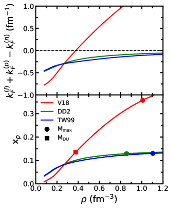
Figure 1: The threshold condition for the DU process (upper panel) and the proton fraction (lower panel) vs. the nucleon density for all chosen EOSs. Markers indicate the $M_{\text{max}}$ configurations and the onset of DU cooling.

II.2 Equation of state

In order to illustrate the relevant properties of the chosen EOSs, we show in Fig. 1 the DU onset condition (upper panel) and the proton fraction (lower panel). One notes that both RMF EOSs predict very similar proton fractions, not allowing the DU process, at variance with the BHF V18 EOS, for which the proton fraction reaches the DU threshold $x_{\text{DU}}=0.135$ at a density $\rho_{\text{DU}}\approx 0.37\;\text{fm}^{-3}$. The associated NS mass is $M_{\text{DU}}=1.01M_{\odot}$, hence all NSs described with the V18 EOS can potentially cool very fast. This is extensively illustrated in the next section.

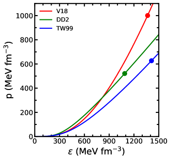
Figure 2: EOSs used in this work. Markers indicate the $M_{\text{max}}$ configurations.

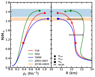
Figure 3: NS gravitational mass vs central baryon density (left) and radius (right) for the different EOSs. Dots indicate the configurations of $M_{\text{max}}$, and stars those of vanishing p1S0 BCS gap in the NS center. Observational constraints on masses et al. (2020); Romani et al. (2022) and from NICER Miller et al. (2021) are included.

In Fig. 2 the final EOS is plotted, i.e., pressure vs. energy density, after imposing beta-stability and charge neutrality conditions, whereas in Fig. 3 we display the resulting NS mass-radius and mass-central density relations, obtained by solving the Tolman-Oppenheimer-Volkoff equations. We stress that the value of the maximum mass for all the selected EOSs is compatible with the current observational lower limits Demorest et al. (2010); Antoniadis et al. (2013); et al. (2016); Cromartie et al. (2019); the recent data $M=2.35\pm 0.17M_{\odot}$ for PSR J0952-0607 Romani et al. (2022) is very constraining, and would actually exclude the TW99 EOS. We also mention the combined estimates of the mass and radius of the isolated pulsar PSR J0030+0451 observed recently by NICER, $M=1.44^{+0.15}_{-0.14}M_{\odot}$ and $R=13.02^{+1.24}_{-1.06}\,$km Miller et al. (2019); Riley et al. (2019), or $M=1.36^{+0.15}_{-0.16}M_{\odot}$ and $R=12.71^{+1.14}_{-1.19}\,$km Miller et al. (2021); Riley et al. (2021), and in particular the result of the combined GW170817+NICER analysis Miller et al. (2021), $R_{2.08}=12.35\pm 0.75$km and $R_{1.4}=12.45\pm 0.65$km, with which only the V18 EOS would fully comply, see Fig. 3 and Table 1.

II.3 Pairing gaps

One of the most important nuclear physics input for the NS cooling simulations are the superfluid properties of stellar matter, basically the neutron and proton pairing gaps in the different reaction channels Yakovlev et al. (2001); Sedrakian and Clark (2019); Burgio et al. (2021). Usually the most important ones are the proton 1S0 (p1S0) and neutron 3PF2 (n3P2) pairing channels; the proton 3PF2 gap is often neglected due to its uncertain properties at large densities, while the neutron 1S0 gap in the crust is of little relevance for the cooling.

These superfluids are created by the formation of $pp$ and $nn$ Cooper pairs due to the attractive part of the $NN$ potential, and are characterized by a critical temperature $T_{c}\approx 0.567\Delta$. The occurrence of pairing when $T<T_{c}$ leads on one hand to an exponential reduction of the emissivity of the neutrino processes the paired component is involved in, and on the other hand to the onset of the “pair breaking and formation” (PBF) process with associated neutrino-antineutrino pair emission. This process starts when the temperature reaches $T_{c}$ of a given type of baryons, becomes maximally efficient when $T\approx 0.8\,T_{c}$, and then is exponentially suppressed for $T\ll T_{c}$ Yakovlev et al. (2001).

In the simplest BCS approximation, and detailing the more general case of pairing in the coupled 3PF2 channel, the pairing gaps are computed by solving the (angle-averaged) gap equation Amundsen and Østgaard (1985); Baldo et al. (1992); Takatsuka and Tamagaki (1993); Elgarøy et al. (1996); Khodel et al. (1998); Baldo et al. (1998) for the two-component $L=1,3$ gap function,

$$\left(\!\!\!\begin{array}[]{l}\Delta_{1}\\ \Delta_{3}\end{array}\!\!\!\right)\!(k)=-\frac{1}{\pi}\int_{0}^{\infty}\!\!dk^{\prime}{k^{\prime}}^{2}\frac{1}{E(k^{\prime})}\left(\!\!\!\begin{array}[]{ll}V_{11}\!\!&\!\!V_{13}\\ V_{31}\!\!&\!\!V_{33}\end{array}\!\!\!\right)\!(k,k^{\prime})\left(\!\!\!\begin{array}[]{l}\Delta_{1}\\ \Delta_{3}\end{array}\!\!\!\right)\!(k^{\prime})$$ (4)

with

$$E(k)^{2}=[e(k)-\mu]^{2}+\Delta_{1}(k)^{2}+\Delta_{3}(k)^{2}\>,$$ (5)

while fixing the (neutron or proton) density,

$$\rho=\frac{k_{F}^{3}}{3\pi^{2}}=2\sum_{k}\frac{1}{2}\left[1-\frac{e(k)-\mu}{E(k)}\right]\>.$$ (6)

Here $e(k)=k^{2}\!/2m$ is the s.p. energy, $\mu\approx e(k_{F})$ is the chemical potential determined self-consistently from Eqs. (4–6), and

$$V_{LL^{\prime}}(k,k^{\prime})=\int_{0}^{\infty}\!dr\,r^{2}\,j_{L^{\prime}}(k^{\prime}\!r)\,V^{TS}_{LL^{\prime}}(r)\,j_{L}(kr)$$ (7)

are the relevant potential matrix elements ($T=1$ and $S=1$; $L,L^{\prime}=1,3$ for the 3PF2 channel, $S=0$; $L,L^{\prime}=0$ for the 1S0 channel) with the bare potential $V$. The relation between (angle-averaged) pairing gap at zero temperature $\Delta\equiv\sqrt{\Delta_{1}^{2}(k_{F})+\Delta_{3}^{2}(k_{F})}$ obtained in this way and the critical temperature of superfluidity is then $T_{c}\approx 0.567\Delta$.

At this simplest level of approximation, the gap is a universal function of the particle density, $\Delta_{\text{BCS}}(\rho)$, and thus valid for any EOS, independent of the $NN$ interaction used, provided that the associated $NN$ phase shifts are reproduced Lombardo and Schulze (2001); Sedrakian and Clark (2006). However, in-medium effects might strongly modify these BCS results, as both the s.p. energy $e(k)$ and the interaction kernel $V$ itself might include the effects of three-body forces and polarization corrections. It turns out that in the p1S0 channel all these corrections lead to a suppression of both magnitude and density domain of the BCS gap, see, e.g, Zhou et al. (2004); Baldo and Schulze (2007) in the BHF context, or Lombardo and Schulze (2001); Sedrakian and Clark (2019); Burgio et al. (2021) for a collection of different theoretical approaches.

The situation is much worse for the gap in the n3P2 channel, which already on the BCS level depends on the $NN$ potential Takatsuka and Tamagaki (1993); Baldo et al. (1998); Khodel et al. (1998); Maurizio et al. (2014); Srinivas and Ramanan (2016); Drischler et al. (2017), as at high density there is no constraint by the $NN$ phase shifts. Furthermore TBF act generally attractive in this channel, but effective mass and quasiparticle strength reduce the gap, and polarization effects on $V$ might be of both signs, in particular in asymmetric beta-stable matter Khodel et al. (2004); Zhou et al. (2004); Schwenk and Friman (2004); Dong et al. (2013); Ding et al. (2016); Drischler et al. (2017); Papakonstantinou and Clark (2017); Ramanan and Urban (2021); Krotscheck et al. (2023, 2024). Note that most theoretical investigations so far consider only pure neutron matter. Thus, due to the high-density nature of this pairing, the various medium effects might be very strong and competing, and there is still no reliable quantitative theoretical prediction for this gap. The most recent investigation Krotscheck et al. (2023, 2024) points to a complete disappearance of the gap, but previous works predict enhancement instead Khodel et al. (2004); Zhou et al. (2004); Drischler et al. (2017).

Further important ingredients in the cooling simulations are the neutron and proton effective masses, which we actually used in Taranto et al. (2016). In the BHF approach, the effective masses can be expressed self-consistently in terms of the s.p. energy $e(k)$ Baldo et al. (2014b),

$$\frac{m^{*}(k)}{m}=\frac{k}{m}\left[\frac{de(k)}{dk}\right]^{-1}\>.$$ (8)

We actually found Taranto et al. (2016); Wei et al. (2020) that their effect can be absorbed into a rescaling of the 1S0 BCS pairing gap, which we perform by introducing global scaling factors $s_{y}$ and $s_{x}$ on both magnitude and extension of the gap, i.e.,

$$\Delta(\rho)\equiv s_{y}\Delta_{\text{BCS}}(\rho/s_{x})\>.$$ (9)

As in Wei et al. (2020), also in this paper we employ the same procedure, and $s_{y},s_{x}$ will be considered as free parameters in the cooling calculations. Their optimal values will be determined later in a combined analysis of cooling data and deduced NS mass distributions.

To illustrate the important role played by the superfluidity gaps, we first evaluate over which range of baryon density inside a NS they are effective. The starred markers in Fig. 3 label the configurations $M_{1S0}$, for which the BCS p1S0 gap vanishes in the NS center, i.e., $M<M_{1S0}$ stars are superfluid throughout, whereas for $M>M_{1S0}$ there is a growing non-superfluid core region. We see an important difference among the three EOS: whereas for the V18 $M_{1S0}=1.92M_{\odot}$ and thus for heavier stars proton superfluidity is only partially present, in the RMF cases the proton gap is fully active in all configurations. Just as the absence of DU cooling, also this feature is due the small proton fractions of the RMF models, which causes relatively small proton partial densities. Thus in this case NS cooling proceeds through the MU and BS processes, modulated by superfluidity.

However, the parameter $s_{x}$ changes the active range of pairing, and this is illustrated in Fig. 4 for the chosen EOSs, which shows the p1S0 gaps in NS matter for several combinations of the scaling parameters $(s_{x},s_{y})$. In each panel we display the central densities for several NS masses (vertical lines) and the mass ranges (shaded regions, only V18) in which DU cooling is suppressed by the p1S0 gap. Due to the smaller proton fractions, the gap extension over the baryon density range is larger for both RMF models than the V18, such that for $s_{x}\geq 1$ pairing is always fully active in all stellar configurations. For the V18 on the contrary, for any choice of $s_{x}$, there are always heavy NSs in which the DU process is unblocked, causing very rapid cooling. This is essential for the confrontation with cooling data in the next section.

Table 2: NS matter baryon densities $\rho_{1S0}$ for the vanishing of the p1S0 gap and corresponding NS masses $M_{1S0}$ with that central density, as a function of the scale parameter $s_{x}$.

EOS	$s_{x}$	$\rho_{1S0}$ $[\!\;\text{fm}^{-3}]$	$M_{1S0}$ [$\!M_{\odot}$]
V18	0.2	0.300	0.70
	0.4	0.388	1.11
	0.6	0.467	1.46
	0.8	0.536	1.73
	1.0	0.599	1.92
	1.2	0.657	2.06
	1.4	0.711	2.16
DD2	0.2	0.307	1.07
	0.4	0.495	2.06
	0.6	0.678	2.38
	0.8	0.861	2.44
	1.0	1.044
	1.2	1.227
	1.4	1.412
TW99	0.2	0.315	0.75
	0.4	0.521	1.54
	0.6	0.710	1.91
	0.8	0.892	2.05
	1.0	1.073	2.09
	1.2	1.254
	1.4	1.436

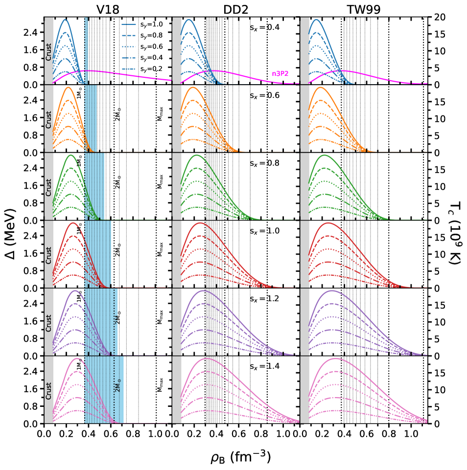
Figure 4: The BCS p1S0 pairing gap in NS matter as a function of baryon density for the adopted EOSs, with different scale factors $s_{x}$ and $s_{y}$ applied, Eq. (9). The shaded areas (only V18) indicate the density range in which the DU process is blocked by superfluidity. Vertical dotted lines indicate the central densities for different NS masses $M/\!M_{\odot}=1.0,1.1,1.2,\ldots$ up to the maximum mass. The unscaled n3P2 BCS gap is also shown in the upper panels.

In Table 2 we summarize the values of the (central) density at which the p1S0 gap disappears, $\rho_{1S0}$, and the corresponding NS mass $M_{1S0}$, for several values of the scaling factor $s_{x}$. For completeness, we also display the unscaled n3P2 BCS gap in the upper panels of Fig. 4. It extends over the entire mass and density range, and therefore would block all cooling processes for all NSs. However, the competing n3P2 PBF process provides too strong cooling for old objects, in disagreement with some data, as found in Grigorian and Voskresensky (2005); Wei et al. (2020) and confirmed in the following section.

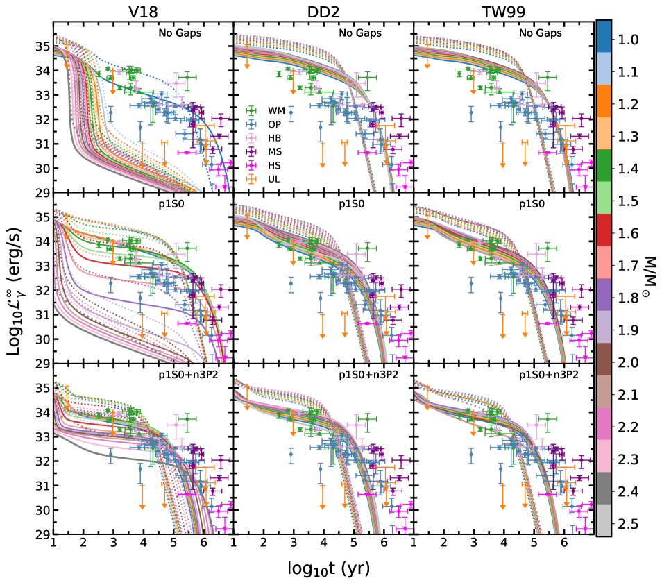
Figure 5: Cooling diagrams obtained with different EOSs (columns) without superfluidity gaps (upper row), with p1S0 gap (middle row), and with p1S0+n3P2 pairing gaps (lower row), for different NS masses $M/\!M_{\odot}=1.0,1.1,\ldots,M_{\text{max}}$ (decreasing curves). The solid (dashed) curves are obtained with a Fe (light elements) atmosphere. The data points are from Potekhin et al. (2020); Coo . See text for details.

III Cooling simulations

For the NS cooling simulations we employ the widely known one-dimensional code NSCool Page , based on an implicit scheme developed in Henyey et al. (1964) for solving the general-relativistic equations of energy balance and energy transport,

$$\frac{1}{4\pi r^{2}}\sqrt{1-\frac{2Gm}{r}}e^{-2\phi}\frac{\partial}{\partial r}(e^{2\phi}L)=-Q_{\nu}-\frac{C_{v}}{e^{\phi}}\frac{\partial T}{\partial t}\>,$$ (10)

$$\frac{L}{4\pi r^{2}}=-\kappa\sqrt{1-\frac{2Gm}{r}}e^{-\phi}\frac{\partial}{\partial r}(e^{\phi}T)\>.$$ (11)

Local luminosity $L$ and temperature $T$ depend on the radial coordinate $r$ and time $t$. The metric function is denoted by $\phi$, whereas $Q_{\nu}$, $C_{v}$, and $\kappa$ are the neutrino emissivity, the specific heat capacity, and the thermal conductivity, respectively.

The code solves the partial differential equations on a grid of spherical shells. The simulation is performed by artificially dividing the star into two parts at an outer boundary given by the radius $r_{b}$ and density $\rho_{b}=10^{10}\,\text{g/cm}^{3}$. At $\rho<\rho_{b}$, the so-called envelope Beznogov et al. (2021) includes the mass and composition change, for instance, due to the accretion, and is solved separately in the code. Here, we use the envelope model obtained in Potekhin et al. (1997). At $\rho>\rho_{b}\ (r<r_{b})$, the matter is strongly degenerate and thus the structure of the star is supposed to be unchanged with time. As a result, we obtain for a NS of given mass and composition of the envelope, a set of cooling curves showing the luminosity $L$ as a function of NS age $t$. Each simulation starts with a constant initial temperature profile, $\tilde{T}\equiv Te^{\phi}=10^{10}\,$K, and ends when $\tilde{T}$ drops to $10^{4}\,$K. Regarding the most important ingredient – neutrino emissivity, this code comprises all relevant cooling reactions: nucleonic DU, MU, BS, and PBF, including modifications due to p1S0 and n3P2 pairing. Moreover, various processes in the crust are included, such as the most important electron-nucleus bremsstrahlung, plasmon decay, electron-ion bremsstrahlung, etc.

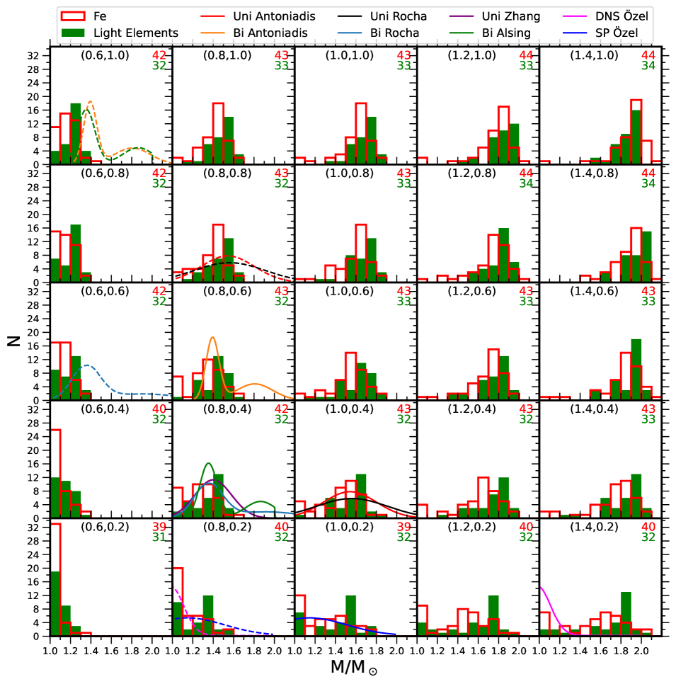
Figure 6: Deduced NS mass distributions for scaling factors $(s_{x}=0.6,\ldots,1.4)\otimes(s_{y}=0.2,\ldots,1.0)$ and with Fe (open red histograms) or light-elements (solid green histograms) atmosphere. $N$ is the number of data points lying in a given mass interval $\Delta M=0.1M_{\odot}$ in the proper ($s_{x},s_{y}$) cooling diagram. Several panels show the best-fit theoretical results Zhang et al. (2011); Antoniadis et al. (2016); Alsing et al. (2018); Rocha et al. (2019); Özel et al. (2012) of Fig. 7 superimposed, using solid (dashed) lines for the Fe (light-elements) results. The top-right numbers indicate the number of data points in the histograms.

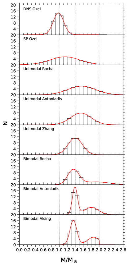
Figure 7: Theoretical NS mass distributions Zhang et al. (2011); Antoniadis et al. (2016); Alsing et al. (2018); Rocha et al. (2019); Özel et al. (2012) (red curves) binned in the same way as Fig. 6 (black histograms). The normalization is to 51 points. Vertical lines indicate $M=1.0,1.4,2.0M_{\odot}$.

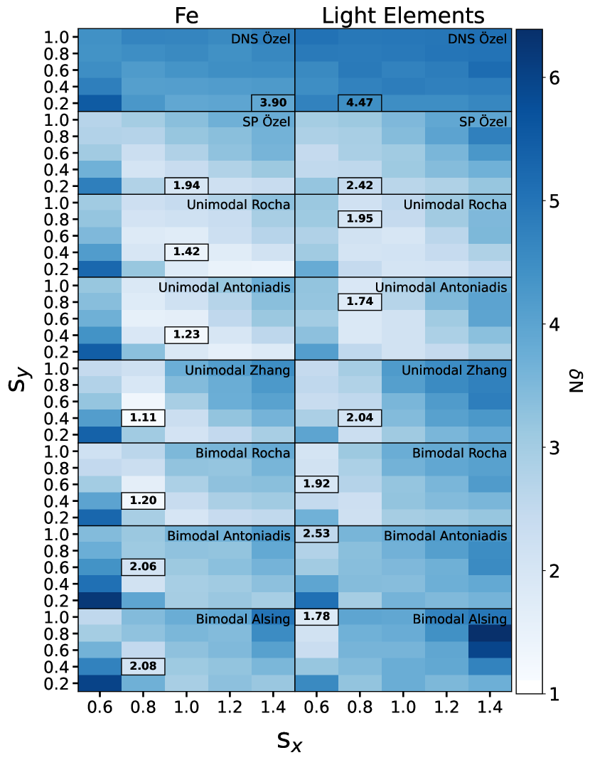
Figure 8: Root-mean-square variances, Eq. (12), between deduced NS mass distributions and various theoretical distributions (shown in Fig. 7), obtained with different p1S0 gap scale factors $s_{x},s_{y}$ for a Fe or light-elements atmosphere. Preferred values are indicated in squared boxes.

In Fig. 5 we show the cooling diagrams obtained with the different EOSs, employing a Fe atmosphere (solid curves) or a light-elements atmosphere (dashed curves), in comparison with the currently known data points Beznogov and Yakovlev (2015a); Potekhin et al. (2020); Coo (with partially large (estimated) error bars), namely for weakly-magnetized NSs (WM, green), ordinary pulsars (OP, blue), high-magnetic-field-B pulsars (HB, pink), the magnificent seven (MS, violet), small hot spots (HS, magenta), and upper limits (UL, orange). There are altogether 57 data points, but we do not use the 6 UL data for the following analyses.

The upper row displays the results obtained without superfluidity. One notes the strong effect of the DU process in the V18 EOS characterized by a far too rapid cooling for all NSs with $M>M_{\text{DU}}=1.01M_{\odot}$, which is clearly unrealistic. On the contrary the DD2 and TW99 EOSs without DU process produce too slow cooling for middle-aged objects and too fast for old objects. Thus the assumption of no superfluidity appears inconsistent with both including or not the DU process, regardless of the atmosphere model.

Accordingly in the middle row we include the p1S0 BCS ($s_{x}=s_{y}=1$) gap. Their main effect is the quenching of the DU process for the V18 EOS, such that stars in the overlap zone $1.01M_{\odot}=M_{\text{DU}}<M<M_{1S0}=1.92M_{\odot}$ cool moderately fast now, and only high-mass stars, $M>1.92M_{\odot}$, cool very rapidly. Altogether a very satisfying coverage of the data is achieved, also taking advantage of the two atmosphere models. In fact all data points can be covered within their error bars. On the contrary, both no-DU models can still not explain most data.

In the lower row we investigate the effect of the n3P2 BCS gap: This extends over the entire density range, and therefore blocks DU processes for all NSs. On the other hand the competing n3P2 PBF process provides a too strong cooling for the old ($\gtrsim 10^{6}$yr) objects Wei et al. (2020), with or without DU process, as already found by other authors Grigorian and Voskresensky (2005); Beznogov and Yakovlev (2015a, b); Beznogov et al. (2018); Potekhin et al. (2019, 2020); Wei et al. (2020).

In conclusion, an EOS featuring DU cooling for a wide enough mass range of NSs together with (partial) quenching by the p1S0 BCS gap seems to be required to reproduce the cooling data. It seems difficult to accommodate finite n3P2 pairing in this setup. We therefore continue the analysis with the V18 EOS including p1S0 pairing but without n3P2 pairing.

IV Gaps and mass distributions

Currently no information on the actual masses of the various cooling objects is available, hence a comparison between theoretically predicted masses and the actual masses of the cooling diagram is not possible. In this situation we can derive a NS mass distribution that is consistent with the outcome of a given cooling simulation by simply counting the number of data points that fall into a given interval between two adjacent fixed-$M$ cooling curves Wei et al. (2019, 2020). (Error bars are disregarded at this level of investigation). The resulting histogram can be compared with mass distributions of NSs obtained in different, independent theoretical ways Zhang et al. (2011); Özel et al. (2012); Kiziltan et al. (2013); Antoniadis et al. (2016); Alsing et al. (2018); Rocha et al. (2019); Landry and Read (2021).

In doing so, we assume that the mass distribution of isolated NSs in the cooling diagram is not different from the mass distributions of NSs in binary systems Zhang et al. (2011); Antoniadis et al. (2016); Alsing et al. (2018); Rocha et al. (2019); Farrow et al. (2019) or all NSs in the Universe, and that the detection of these sources is independent of their brightness; both of these assumptions being highly unlikely to be fulfilled. A further principal problem is the lack of information on the atmosphere of the data objects, which requires further theoretical assumptions in this analysis, the simplest one being to use a fixed atmosphere model.

In attendance of future improvement of information on the data sources, we proceed nevertheless with this way of derivation of the mass distribution: The masses of the 51 cooling data points are assumed to be those predicted theoretically by their position in the cooling diagrams among the theoretical curves displayed in Fig. 5, and Fig. 6 shows the resulting mass histograms for different choices of the p1S0 pairing parameters ($s_{x},s_{y}$), assuming either a common Fe (open histograms) or a light-elements atmosphere (solid histograms) for all data points. This is clearly unrealistic, and in fact in the first case up to 44 and in the second case up to 34 of the 51 sources can be fitted, while a fit of more data would require a suitable choice of atmosphere for each object. In this case only 4 objects would remain out of this analysis for the best parameter choices (but their errors bars still reach the external theoretical curves): Calvera, J0806, J2143, J1154.

One observes that increasing $s_{x}$ or to a lesser degree $s_{y}$ shifts the centroid of the derived mass distributions to higher values, since the cooling curves move upwards due to the increased suppression of the DU process, as shown in Fig. 4 of Wei et al. (2020).

The different results in Fig. 6 can now be compared with other theoretical studies of the NS mass distribution Zhang et al. (2011); Özel et al. (2012); Kiziltan et al. (2013); Antoniadis et al. (2016); Alsing et al. (2018); Rocha et al. (2019), in particular unimodal or bimodal distributions, which were derived on the basis of distinct evolutionary paths and accretion episodes. In this paper we also include the analysis Özel et al. (2012) for double neutron stars (DNS) and slow pulsars (SP). Fig. 7 contains a compilation of the theoretical mass distributions that we use for comparison. We provide a binning and normalization consistent with Fig. 6 in order to confront directly with our results. For a quantitative comparison we simply compute the rms deviations between the histograms $\{N_{i}^{\text{dat}}\}$ in Fig. 6 and $\{N_{i}^{\text{theo}}\}$ in Fig. 7,

$$\delta N\equiv\sqrt{\frac{1}{N^{\text{dat}}}\sum_{i}\Big{(}N_{i}^{\text{dat}}-N_{i}^{\text{theo}}\Big{)}^{2}}\>,$$ (12)

where $i$ labels the mass bins and $N^{\text{dat}}=51$ is the total number of data points excluding the UL markers.

The results are visualized in the heatmap shown in Fig. 8 for the various combinations, where we also indicate the optimal values $s_{x},s_{y}$ for each theoretical mass distribution and the two atmosphere models separately. Of course the use of a unique atmosphere model for the whole data set is unrealistic, but currently impossible to overcome without further constraints on the data. Nevertheless some qualitative conclusions can be drawn:

For a Fe atmosphere the best agreement with the considered distributions seems to require values of $s_{x}\approx 0.8$–$1.0$ and $s_{y}\approx 0.4$, which would also be consistent with microscopic investigations of the 1S0 pairing gap, as discussed before. The quality of agreement is worst for the DNS Özel one, which favors a very large $s_{x}$. In Fig. 6 [panels (0.8,0.2) and (1.4,0.2)] it can clearly be seen that the median of this distribution is far too low compared to the data. The best overall fit is provided by the Unimodal Zhang distribution (median $\sim 1.4M_{\odot}$) and $(0.8,0.4)$. The corresponding panel in Fig. 6 shows a decent agreement between open histogram and lila curve, confirming the numerical analysis. Also Unimodal Antoniadis and Bimodal Rocha distributions provide fits of similar quality.

For a light-elements atmosphere, all theoretical models single out $s_{x}=0.6$–$0.8$ as preferred value, but no definite value of $s_{y}$. The quality of the fits is worse than for the Fe atmosphere, and also less data points are comprised in the analysis (31–34) than for the Fe atmosphere (39–44).

The ($s_{x},s_{y}$) configurations which fit best a given theoretical model, have that theoretical curve superimposed in Fig. 6, and four of the models single out (0.8,0.4) as ‘best’ parameter set.

We conclude that in nearly all cases the comparison between cooling diagrams and population models indicates a reduction of the pairing range to $s_{x}\approx 0.8$ and also a reduction of the magnitude $s_{y}\approx 0.4$, which is however less well determined and more model dependent. This agrees qualitatively well with theoretical estimates of the reduction of the BCS gap by medium effects Burgio et al. (2021). While bimodal distributions appear slightly disfavored, the current limitations of theoretical method and available data do not allow to clearly single out a preferred theoretical population model, though. In particular, we stress again a probable selection effect that would make heavy and faint NSs unobservable and thus not appear in the high-mass part of the histograms. This would put a bias on a too low centroid of the derived mass distributions and accordingly too strong suppression of the p1S0 gap. But it is currently impossible to quantify this assertion, and our analysis remains at an exploratory state.

V Conclusions

We have presented a global combined analysis of NS cooling and mass distributions, employing the most recent set of cooling data. We confirm that those data demand a fast cooling mechanism like the DU process (or alternative scenarios Grigorian and Voskresensky (2005); Blaschke and Grigorian (2007); Blaschke et al. (2013); Shternin et al. (2018); Suleiman et al. (2023) not considered in this work). This imposes an important constraint on the proton fraction and symmetry energy of a realistic nucleonic NS EOS, complementary to those obtained from nuclear structure, global NS observables, and recent gravitational wave observations. We employed here the V18 BHF EOS that fulfills all these constraints and predicts DU cooling for even the lightest NSs.

Cooling can then be modulated by the strength of the p1S0 pairing gap, while the PBF process associated with n3P2 pairing seems to provide too strong cooling for a satisfactory reproduction of the data. The best simultaneous reproduction of various theoretical NS mass distributions is possible with a p1S0 gap slightly reduced in magnitude and density extension, in qualitative agreement with theoretical investigations of that gap, while the disappearance of the n3P2 gap is also supported by recent theoretical investigations.

Currently this method is hampered by missing information on masses and atmospheres of the cooling data, which will constitute very effective constraints in the future. This and more abundant cooling data will also allow to pin down the density range (onset density) of (blocked) DU cooling in the EOS, which is another important degree of freedom that was not studied in this work.

Our general framework was a purely nucleonic scenario, and exotic types of matter like hyperons or quark matter were not considered in this work. Those still present a formidable challenge to cooling calculations due to their largely unknown microphysics ingredients relevant for cooling, like cooling rates, heat capacities, transport properties, and most of all superfluid properties.