Perturbative QCD meets phase quenching: The pressure of cold Quark Matter

Abstract

Nonperturbative inequalities constrain the pressure of Quantum Chromodynamics (QCD) with its phase-quenched version, a Sign-Problem-free theory amenable to lattice treatment. In the perturbative regime with a small QCD coupling constant $\alpha_{s}$, one of these inequalities manifests as an $O(\alpha_{s}^{3})$ difference between the phase-quenched and QCD pressures at large baryon chemical potential $\mu_{\text{B}}$. In this work, we generalize state-of-the-art algorithmic techniques in vacuum quantum field theory to address large-scale multiloop computations at finite chemical potential. Using this approach, we evaluate this $O(\alpha_{s}^{3})$ difference and show that it is a gauge-independent and small positive number compared to the known perturbative coefficients at this order. This implies that phase-quenched lattice simulations can provide a complementary nonperturbative method for accurately determining the pressure of cold and dense quark matter at $O(\alpha_{s}^{3})$.

Introduction.—Determining the bulk thermodynamic properties of strongly interacting matter at the highest temperatures and densities reached in Nature is one of the major challenges in theoretical physics. At high temperatures and small baryon densities, experiments conducted with ultrarelativistic heavy-ion collisions (see e.g. [1] for a review) and theoretical work using nonperturbative lattice simulations [2, 3] have been crucial in understanding the equilibrium properties of Quantum Chromodynamic (QCD) matter. Simultaneously to these developments, the past decade has witnessed rapid progress in the study of neutron stars (NSs). Due to the tight link between NS-matter microphysics and the macroscopic properties of the stars, NSs have become unique cosmic laboratories for studying dense QCD matter (see e.g. [4] for a review). What makes them particularly fascinating in the context of strongly interacting physics is that, unlike any other accessible system in the Universe, the maximal densities reached inside the cores of massive NSs may exceed the limit where nuclear matter undergoes a transition into deconfined cold quark matter (QM) [5, 6].

To describe the thermodynamic properties of dense QCD matter in equilibrium, one needs information about the equation of state (EOS), which relates the pressure $p$ to energy density. Ideally, the EOS should be determined using nonperturbative lattice field theory tools that have provided accurate results in collider environments. Unfortunately, the standard Monte Carlo (MC) techniques fail at finite baryon density due to the Sign Problem [7, 8, 9, 10, 11], which prevents lattice QCD simulations in the region of low temperature $T$ and large baryon chemical potential $\mu_{\text{B}}$. Consequently, the only practical methods available to reliably describe the EOS of cold and dense QCD matter are limited to Chiral Effective Theory, applicable at densities around the nuclear matter saturation density [12, 13, 14, 15], and weak-coupling perturbative QCD within high-density QM [16, 17, 18, 19, 20, 21, 22]. Several studies [23, 24, 5, 25, 26, 27, 28, 6] have shown that systematic interpolations between low- and high-density regions, combined with information from astrophysical NS observations [29, 30, 31, 32, 33, 34], can effectively constrain the behavior of the EOS across all densities, provided that accurate asymptotic limits are established at both ends.

Additionally, further bounds for the dense QCD matter EOS can be obtained using phase-quenched (PQ) lattice QCD [35]. In the phase-quenched approximation, the fermion determinant in the QCD partition function for a quark with flavor $f$, nonzero mass $m_{f}$, and chemical potential $\mu_{f}$ is replaced by its magnitude

$$\begin{split}\det(\mathcal{D}(\mu_{f}))&\to|\det(\mathcal{D}(\mu_{f}))|\\ &=\sqrt{\det(\mathcal{D}(\mu_{f}))\det(\mathcal{D}(-\mu_{f}))},\end{split}$$ (1)

where the Dirac operator $\mathcal{D}(\mu_{f})\equiv\not{D}+m_{f}+\mu_{f}\gamma^{0}$, and the last equality follows from its $\gamma^{5}$-hermiticity. Here, each phase-quenched fermion corresponds to two copies of “half-species”, appearing in pairs with equal mass but opposite chemical potential. Although this formulation is unphysical, it can constrain the physically more interesting scenarios involving finite $\mu_{\text{B}}$.

For example, consider QCD with two degenerate flavors of light up and down quarks, and a baryon chemical potential $\mu_{u}=\mu_{d}=\mu_{\text{B}}/3$. In such a scenario, it follows from Eq. 1 that the phase-quenched partition function is equivalent to the partition function of QCD with a nonzero isospin chemical potential $\mu_{\text{I}}$, where $\mu_{u}=-\mu_{d}=\mu_{\text{I}}/2$. Using this observation and nonperturbative QCD inequalities [36], Cohen showed in [37] that the phase-quenched pressure of isospin matter $p_{\text{PQ}}$ serves as a strict upper bound on the QCD pressure of baryonic matter $p$, i.e. $p_{\text{PQ}}(3\mu_{\text{I}}/2)\geq p(\mu_{\text{B}})$.

In NS interiors, the energy density may be sufficiently high to give rise to the onset of strange quarks, either in the form of hyperons or three-flavor QM. Chemical equilibrium under weak interactions (beta-equilibrium) with a nonzero strange quark mass requires $\mu_{d}=\mu_{s}$ and $\mu_{d}>\mu_{u}$. In this context, Fujimoto and Reddy demonstrated in [38] that a similar bound to the two-flavor case can be derived for the pressure at nonzero $\mu_{\text{B}}$ and $\mu_{\text{I}}$, utilizing additional nonperturbative QCD inequalities derived in [39]. This inequality necessitates $\mu_{\text{I}}$ as a function of $\mu_{\text{B}}$, which remains unknown unless certain model-dependent assumptions are made.

In [40], Moore and Gorda recently noted that the phase-quenched formulation applies to any arbitrary linear combination of chemical potentials, not limited to $\mu_{\text{I}}$. They suggested that conducting phase-quenched lattice simulations with three-flavor QM could be the most effective method to constrain the NS EOS. Although this phase-quenched configuration of quark chemical potentials represents a completely unphysical system, it holds the potential to provide the most stringent bounds on the physical NS EOS. In particular, at high densities the relative difference between the phase-quenched pressure and the QCD pressure $p_{\text{PQ}}-p$ is perturbatively order $\alpha_{s}^{3}$ in the QCD coupling constant. In any $\mu$-region where this leading $O(\alpha_{s}^{3})$ correction is small, it can be combined with $p_{\text{PQ}}$ to provide an improved estimate of $p$. This estimation would be perturbatively complete up to higher-order corrections in $\alpha_{s}$ and nonperturbative effects such as pairing gaps [41, 42, 43, 44].

In this Letter, we explicitly evaluate this leading perturbative $O(\alpha_{s}^{3})$ correction. We show that this correction, originating from a single four-loop diagram with two fermion loops connected by three gluons, is a gauge-independent and small positive number compared to the known perturbative coefficients at this order [22]. Hence, phase-quenched lattice simulations can offer a complementary nonperturbative method for accurately determining the pressure of cold and dense quark matter at $O(\alpha_{s}^{3})$. Our diagrammatic evaluation is achieved by generalizing state-of-the-art algorithmic techniques in vacuum quantum field theory to tackle large-scale multiloop computations at finite chemical potential. This includes an analytical computation of the fermionic and bosonic momentum integrals for the zero-components, followed by the numerical MC evaluation of the remaining multi-dimensional spatial momentum integrals. This work represents the first-ever computation of a two-particle-irreducible (2PI) four-loop diagram at finite $\mu$, paving the way toward large-scale automatization of multi-loop computations in the context of field theory at finite density.

Setup of the calculation.—In the context of cold and dense QM with $N_{f}$ quark flavors, the pressure is given in the grand canonical ensemble by $p=-\Omega$, with Euclidean partition function

$$\mathcal{Z}(\{\mu_{j}\})=\int\mathcal{D}A\,e^{-S[A]}\prod^{N_{f}}_{j=1}\det(\mathcal{D}(\mu_{j})).$$ (2)

The perturbative expansion of the pressure then follows as the sum of all connected vacuum Feynman diagrams. The phase-quenched version of this theory makes use of the replacement in Eq. 1, which can be integrated via

$$\sqrt{\det{\mathcal{D}(\pm\mu_{j})}}=\exp{\biggl{\{}\frac{1}{2}\text{tr}\,\log{\mathcal{D}(\pm\mu_{j})}\biggr{\}}}.$$ (3)

The corresponding Feynman rule derived from here amounts to averaging over the sign of each of the quarks’ chemical potentials. To see the consequences of this averaging, consider a vacuum-type Feynman diagram $\mathcal{G}(\{\mu_{j}\})$ in QCD with fermion momenta $P=(P^{0}+i\mu_{j},\vec{p})$ and bosonic momenta $Q=(Q^{0},\vec{q})$. Upon the replacement $\mu_{j}\to-\mu_{j}$ for all quarks in $\mathcal{G}$ (i.e. take the complex conjugate), one can make use of the integral’s symmetry under flipping the signs of all the fermionic and bosonic loop momenta and the Euclidean QCD Feynman rules to obtain

$$\mathcal{G}(\{-\mu_{j}\})=(-1)^{v_{q}+v_{3}}\mathcal{G}(\{\mu_{j}\})=(-1)^{v-v_{4}}\mathcal{G}(\{\mu_{j}\}),$$ (4)

with $v$, $v_{q}$, $v_{3}$, and $v_{4}$ the number of total, quark-gluon, three-gluon, and four-gluon vertices, respectively. Now, a vacuum-type graph in QCD can only have an odd number of total vertices if it contains an odd number of vertices of valency 4, i.e. four-gluon interactions (see e.g. [45]). Hence, the exponent $v-v_{4}$ in Eq. 4 is an even number, leading to $\mathcal{G}(\{-\mu_{j}\})=\mathcal{G}(\{\mu_{j}\})$. This implies two things:

1. Vacuum Feynman diagrams are real numbers,

2. Phase-quenched Feynman rules are equivalent to QCD for diagrams with a single quark loop, vanishing in the difference $p_{PQ}(\{\mu_{j}\})-p(\{\mu_{j}\})$.

Therefore, one expects possible deviations for diagrams containing at least two quark loops.

Let us consider a generic diagram with two quark loops carrying chemical potentials $\mu_{1}$ and $\mu_{2}$, written as

$$\mathcal{G}^{\xi}(\mu_{1},\mu_{2})=\int_{Q_{b}}\mathcal{N}^{\xi}(Q_{b})\Gamma^{(n)}(Q_{b},\mu_{1})\Gamma^{(m)}(Q_{b},\mu_{2}),$$ (5)

where $Q_{b}$ denotes the set of bosonic loop momenta running through the diagram, and $\mathcal{N}^{\xi}(Q_{b})$ contains the color traces and the corresponding bosonic Feynman rules, for general covariant gauges parametrized by $\xi$; $\Gamma^{(n)}$ is an insertion of a gluon $n$-point function with one quark loop (suppressing Lorentz and color indices). From the phase-quenched Feynman rules and the reality of vacuum diagrams, it then follows that the contribution of $\mathcal{G}$ to $p_{\text{PQ}}(\{\mu_{j}\})-p(\{\mu_{j}\})$ is

$$p_{\text{PQ}}-p\biggr{\rvert}_{\mathcal{G}} =-\frac{1}{2}\left[\mathcal{G}^{\xi}(\mu_{1},\mu_{2})-\mathcal{G}^{\xi}(\mu_{1},-\mu_{2})\right]$$

$$=-i\int_{Q_{b}}\mathcal{N}^{\xi}(Q_{b})\Gamma^{(n)}(Q_{b},\mu_{1})\text{Im}\,\Gamma^{(m)}(Q_{b},\mu_{2})$$

$$=\int_{Q_{b}}\mathcal{N}^{\xi}(Q_{b})\text{Im}\,\Gamma^{(n)}(Q_{b},\mu_{1})\text{Im}\,\Gamma^{(m)}(Q_{b},\mu_{2}).$$ (6)

Here, we made use of the fact that bosons do not carry chemical potentials, implying $\mathcal{N}$ is real. One can readily see that the one-loop gluon two-point function, defined as

$$\Gamma^{(2)}_{\alpha\beta}(Q,\mu_{j})=\int_{\{P\}_{j}}\frac{\text{tr}\,\not{P}\gamma_{\alpha}(\not{P}-\not{Q})\gamma_{\beta}}{P^{2}(P-Q)^{2}},$$ (7)

is a real number, as complex conjugation is equivalent to the shift $P\to Q-P$, which is a symmetry of the integral. Here, $\int_{\{P\}_{j}}f(P^{0},\vec{p})\equiv\int\frac{\mathrm{d}^{4}P}{(2\pi)^{4}}f(P^{0}+i\mu_{j},\vec{p})$ denotes the 4-dimensional fermionic loop momentum integral.

It turns out this argument no longer applies to the three-point function, as this integral has no symmetries of this type. One then expects that the leading order contribution to $p_{\text{PQ}}-p$ is a diagram composed of two quark loops connected by three gluon lines, entering at four loops: “the Bugblatter” [46]. In fact, there are two diagrams of this type with differing relative fermion flows, and their explicit expressions using the QCD Feynman rules, up to the terms proportional to $\xi$, are as follows:

$$\begin{split}\raisebox{-0.4pt}{\includegraphics[height=31.2982pt]{B1.png}}&=\frac{g_{s}^{6}}{6}\text{tr}\,(T^{a}T^{b}T^{c})\text{tr}\,(T^{a}T^{b}T^{c})\sum^{N_{f}}_{i,j=1}\biggl{\{}\int_{Q\{P\}_{i}\{R\}^{\text{*}}_{j}S}\frac{-\text{tr}\,[\not{P}\gamma^{\mu}(\not{P}-\not{S})\gamma^{\nu}(\not{Q}-\not{P})\gamma^{\sigma}]\,\text{tr}\,[\not{R}\gamma^{\mu}(\not{R}-\not{S})\gamma^{\nu}(\not{Q}-\not{R})\gamma^{\sigma}]}{Q^{2}P^{2}R^{2}S^{2}(P-S)^{2}(R-S)^{2}(Q-P)^{2}(Q-R)^{2}(Q-S)^{2}}\\ &+\text{$\xi$ -dependent terms}\biggl{\}},\\ \raisebox{-0.4pt}{\includegraphics[height=31.2982pt]{B2.png}}&=\frac{g_{s}^{6}}{6}\text{tr}\,(T^{a}T^{b}T^{c})\text{tr}\,(T^{a}T^{c}T^{b})\sum^{N_{f}}_{i,j=1}\biggl{\{}\int_{Q\{P\}_{i}\{R\}_{j}S}\frac{+\text{tr}\,[\not{P}\gamma^{\mu}(\not{P}-\not{S})\gamma^{\nu}(\not{Q}-\not{P})\gamma^{\sigma}]\,\text{tr}\,[\not{R}\gamma^{\sigma}(\not{Q}-\not{R})\gamma^{\nu}(\not{R}-\not{S})\gamma^{\mu}]}{Q^{2}P^{2}R^{2}S^{2}(P-S)^{2}(R-S)^{2}(Q-P)^{2}(Q-R)^{2}(Q-S)^{2}}\\ &+\text{$\xi$ -dependent terms}\biggl{\}}.\\ \end{split}$$ (8)

Here, we sum over all $N_{f}$ flavors running through each quark loop. Denoting the integral expressions inside the curly brackets for each diagram by $B^{\xi}_{1}(\mu_{i},\mu_{j})$ and $B^{\xi}_{2}(\mu_{i},\mu_{j})$, respectively, the Dirac traces can be related through charge conjugation, giving

$$B^{\xi}_{2}(\mu_{i},\mu_{j})=-B^{\xi}_{1}(\mu_{i},-\mu_{j}).$$ (9)

This is just a manifestation of Furry’s theorem, as pointed out in [40].

Moreover, in terms of the $\text{SU}(N_{c})$ structure constants $f^{abc}$ and the totally symmetric group invariant $d^{abc}$, the color traces entering Eq. 8 are related through complex conjugation:

$$\text{tr}\,(T^{a}T^{b}T^{c})=\frac{1}{4}(d^{abc}+if^{abc})=\text{tr}\,(T^{a}T^{c}T^{b})^{\text{*}}.$$ (10)

With these relations at hand, we proceed to construct $p_{\text{PQ}}-p$ as shown above, by averaging over the $N_{f}$ chemical potentials running in the loops, for both diagrams. As instructed in the NS setup, we specialize to the case of asymptotically dense three-flavor $(N_{f}=3)$ unpaired QM in beta-equilibrium, where quarks can be considered massless and quark chemical potentials are equal. We set $\mu_{i}=\mu_{\text{B}}/3$ for all quarks, obtaining altogether

$$\begin{split}p_{\text{PQ}}(\mu_{\text{B}})-p(\mu_{\text{B}})&=\frac{-3^{2}}{6\times 3^{4}}\frac{d^{abc}d^{abc}}{16}g_{s}^{6}\\ &\times\left[B^{\xi}_{1}(\mu_{\text{B}},\mu_{\text{B}})-B^{\xi}_{1}(\mu_{\text{B}},-\mu_{\text{B}})\right]\\ &+O(g_{s}^{8}),\end{split}$$ (11)

where an additional factor of $3^{4}$ appears through the scaling of $B^{\xi}_{1}$ upon replacing $\mu_{i}^{4}$ by $\mu_{\text{B}}^{4}$, and $d^{abc}d^{abc}=(N_{c}^{2}-1)(N_{c}^{2}-4)/N_{c}$. This expression satisfies several properties, as we demonstrate in the following.

Firstly, expanding the diagrams in general covariant gauge in terms of scalarized integrals, one obtains a quadratic polynomial in the gauge parameter $\xi$. At this point, one can already appreciate the complexity of these diagrams, as they contain all nine non-factorized planar QCD vacuum topologies at four loops [47]. Upon exploiting linear relations among these integrals, in the form of momentum shifts stemming from the graphs’ internal symmetries [48, 49], we explicitly checked that the gauge parameter cancels out at the integrand level in the sum entering Eq. 11, rendering this combination gauge invariant. Consequently, in the following, we set $\xi=0$ and drop the superscript $\xi$.

Secondly, we can prove that this expression is automatically positive, as expected from the nonperturbative inequality $p_{\text{PQ}}\geq p$. In effect, the prefactor in Eq. 11 is nonpositive for all $N_{c}$, so it suffices to show that the difference inside the square brackets is negative, a combination being precisely of the form encountered in Eq. 6. As bosonic propagators are real and positive in the whole region of integration, one has

$$\begin{split}B_{1}(\mu_{\text{B}},\mu_{\text{B}})&-B_{1}(\mu_{\text{B}},-\mu_{\text{B}})\\ &=-2\int_{QS}\frac{\left[\text{Im}\,\Gamma^{(3)}_{\mu\nu\sigma}(Q,S,\mu_{\text{B}})\right]^{2}}{Q^{2}S^{2}(Q-S)^{2}}\leq 0,\end{split}$$ (12)

proving that the leading-order contribution to $p_{\text{PQ}}-p$ is positive.

Thirdly, we can argue that it is infrared finite. Indeed, the infrared physics of this diagram is properly captured by the hard-thermal-loop (HTL) limit of the three-gluon vertex function, whose color structure is $\Gamma^{(3)}_{\text{HTL}}\sim f^{abc}$ [20]. As only $d^{abc}$’s enter Eq. 11, this expression must be infrared finite (see also [40]), further implying that non-analytic logarithms in the coupling arising from the HTL resummation can potentially enter only at order $O(\alpha_{s}^{4}\ln^{n}\alpha_{s})$.

Finally, we argue that Eq. 12 is ultraviolet finite. One might expect this based on the observation that there are no lower loop diagrams with the color factor $d^{abc}d^{abc}$ that could renormalize Eq. 11. Indeed, this combination picks up the imaginary part of the vertex function, a quantity that vanishes in the ultraviolet due to this limit being pure vacuum (i.e. $i\mu\to 0$). Thus, only the $f^{abc}f^{abc}$ piece of the Bugblatter diagrams entering full QCD, containing the real part of the vertex function, requires renormalization.

Numerical evaluation.—Let us then concentrate on the evaluation of the finite four-loop momentum integrals displayed in Eq. 12. In modern quantum field theory, multi-loop diagrams are often first expanded in terms of scalarized integrals, which are then systematically reduced to a basis of so-called master integrals through large-scale automated algorithmic procedures [50, 51]. In this context, techniques for computing master integrals in dimensional regularization are highly developed [52]. However, in a thermal setup (finite $\mu$ or $T$) we break Lorentz symmetry, limiting the usage of the traditional methods that have proven successful in the vacuum setting. Despite this, all the relevant thermal cases up to the three-loop level have been computed on a case-by-case basis, often through brute-force calculation [16, 53]. However, only a few of the simplest four-loop integrals are known [54, 55, 56].

Recent developments in high-performance numerical evaluation of vacuum integrals directly in momentum space, such as the Loop-Tree Duality (LTD) (see e.g. [57, 58]), offer a promising alternative avenue to multi-loop integration. The defining feature these techniques capitalize on is the analytical computation of the temporal momentum integrals via the residue theorem. This approach is particularly suitable for finite-density calculations due to the effect of the chemical potentials being entirely encoded in the temporal momentum components.

Inspired by the LTD and related ideas, we put forward a novel generalization of these approaches to finite-density field theory for evaluating our Bugblatter diagrams. Specifically, we implement numerical MC integration routines for the spatial momentum integrals, preceded by an analytical computation of zero-component residues. This is realized by restructuring the integrand into a convenient representation, allowing for the removal of local spurious divergences that hinder direct numerical integration.

In the following, we generalize the derivation of the integral representation presented in [59] to finite $\mu$, employing the notation introduced therein. Let $\mathbf{x}=(x_{i})_{i\in\{1,\dots,n\}}$ denote a vector with $n$ components, $\mathbf{x}\cdot\mathbf{y}=\sum_{i=1}^{n}x_{i}y_{i}$ the standard scalar product of two vectors $\mathbf{x}$ and $\mathbf{y}$, and $\mathbf{x}\odot\mathbf{y}=(x_{i}y_{i})_{i\in\{1,\dots,n\}}$ component-wise multiplication of the vectors. Now, a vacuum-type $l$-loop integral with $n$ single-power propagators at finite $\mu$, stripped of its spatial loop integrations over $\vec{p}_{i}$, can be written as

$$I\equiv\int\prod_{i=1}^{l}\frac{\mathrm{d}P_{i}^{0}}{2\pi}\frac{\mathcal{N}(\mathbf{Q}^{0})}{\prod_{j=1}^{n}\left[\left(Q_{j}^{0}\right)^{2}+E_{j}^{2}\right]},$$ (13)

where the numerator $\mathcal{N}$ is a regular function of the temporal propagator momenta $\mathbf{Q}^{0}=\sum_{i=1}^{l}\mathbf{S}_{i}P_{i}^{0}+i\boldsymbol{\tau}\mu$, the vectors $\mathbf{S}_{i}=(S_{1i},\dots,S_{ni})$ with $S_{ji}\in\{\pm 1,0\}$ fix the loop momentum basis, and the vector $\boldsymbol{\tau}=\sum_{i=1}^{l}\mathbf{S}_{i}\tilde{\tau}_{i}\in\{\pm 1,0\}^{n}$ with $\tilde{\tau}_{i}\in\mathbb{Z}$ determines the fermion signature of each propagator. The propagator energies are given by $E_{j}^{2}=|\vec{q}_{j}|^{2}+m_{j}^{2}$, where the spatial loop momenta are $\vec{\mathbf{q}}=\sum_{i=1}^{l}\mathbf{S}_{i}\vec{p}_{i}$ and the masses are denoted by $m_{j}$.

Next, we apply the residue theorem to perform the temporal integrals over $P_{i}^{0}$ in Eq. 13, resulting in

$$\begin{split}I&=\sum_{\begin{subarray}{c}\boldsymbol{\rho}\in\{\pm 1\}^{n}\\ \boldsymbol{\sigma}\in\{\pm 1\}^{n}\end{subarray}}\mathcal{N}(i\boldsymbol{\sigma}\odot\boldsymbol{\rho}\odot\mathbf{E})\prod_{j=1}^{n}\frac{\Theta(\rho_{j}E_{j}-\sigma_{j}\tau_{j}\mu)}{2\rho_{j}E_{j}}\\ &\quad\times\int_{\mathbb{R}_{+}^{n}}\mathrm{d}\boldsymbol{\alpha}\,\mathrm{e}^{-\boldsymbol{\alpha}\cdot(\boldsymbol{\rho}\odot\mathbf{E})}\prod_{i=1}^{l}\delta\bigl{(}\boldsymbol{\alpha}\cdot(\boldsymbol{\sigma}\odot\mathbf{S}_{i})\bigr{)}.\end{split}$$ (14)

In contrast to the vacuum case, this generalization involves step functions that include $\mu$, along with an additional sum over the sign vectors $\boldsymbol{\rho}$. However, the integral on the second line of Eq. 14, representing a Laplace transform of a non-simplicial convex cone, is an object already encountered in the vacuum computation. We perform this integral using the algorithmic procedure described in [59], leading to a sum of rational functions of linear combinations of the energies $E_{i}$. The resulting representation for the spatial integral is free of spurious divergences, making it particularly suitable for direct numerical integration.

Nonetheless, the expression resulting from Eq. 14 often contains integrable singularities that may deteriorate the MC integration. To mitigate the issue, we have implemented a multi-channeling technique, as presented in [60]. This procedure flattens some of the integrable singularities by expressing the integrand as a sum of multiple terms (i.e. channels), which are then integrated separately. Additionally, we have found that using small but nonzero masses in the energies $E_{j}$ improves the stability of the integration. Selecting $m_{j}=\lambda\mu_{\text{B}}$ with $\lambda=10^{-3}$, we have verified the insensitivity of our results under varying $\lambda\in[10^{-4},10^{-2}]$.

Furthermore, it is important to emphasize that the above procedure is not limited to the current finite four-loop diagrams alone; it is equally applicable to diagrams of various topologies and loop orders. For example, we checked that our approach correctly reproduces known results at two- and three-loop levels. These cases include the subtraction of ultraviolet divergences, a topic we will detail in an upcoming publication.

Results and discussion.—We are now prepared to evaluate the new coefficient in Eq. 12 using the integrand representation generated by Eq. 14. With a suitable choice of coordinates, this leads to a ten-dimensional integral over the spatial momenta. We compute this integral numerically employing the Vegas5.6 integration routine [61], distributing roughly $10^{13}$ MC samples across 75 channels (see above). We determine the new coefficient to be

$$B_{1}(\mu_{\text{B}},\mu_{\text{B}})-B_{1}(\mu_{\text{B}},-\mu_{\text{B}})=-3.3278(14)\cdot 10^{-6}\mu_{\text{B}}^{4},$$ (15)

where the MC error in the obtained numerical result is small. By utilizing Eq. 11 and setting $N_{c}=3$, we then find that the relative difference $p_{\text{PQ}}-p$ in the perturbative region is

$$p_{\text{PQ}}(\mu_{\text{B}})-p(\mu_{\text{B}})=3.3681(14)\cdot\left(\frac{\alpha_{s}(\overline{\Lambda})}{\pi}\right)^{3}p_{\text{free}},$$ (16)

where $\alpha_{s}=\alpha_{s}(\overline{\Lambda})$ represents the renormalized strong coupling constant in the $\overline{\text{MS}}$ scheme at the renormalization scale $\overline{\Lambda}$, and we have written our result in terms of the pressure of a free Fermi gas of quarks in beta equilibrium, denoted as $p_{\text{free}}=3(\mu_{\text{B}}/3)^{4}/4\pi^{2}$.

In Fig. 1, we display the relative difference $p_{\text{PQ}}-p$ normalized by the free quark pressure as a function of $\mu_{\text{B}}$. We employ the known three-loop running for $\alpha_{s}(\overline{\Lambda})$, set $\overline{\Lambda}=2X\mu_{\text{B}}/3$, and estimate the uncertainty arising from truncating the perturbative series by varying $X$ in the range $[1/2,2]$. It is observed that in the perturbative region $\mu_{\text{B}}\gtrsim 2.5$ GeV, corresponding to $\alpha_{s}\lesssim 0.5$, the difference $p_{\text{PQ}}-p$ is very small. This implies that phase-quenched lattice simulations provide an accurate approximation for the dense QM pressure in the perturbative regime.

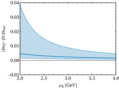
Figure 1: The leading-order difference between the pressure of three-flavor dense QM and its phase-quenched version, normalized by the free pressure, as a function of the baryon chemical potential. The shaded region shows the scale variation of $X\in[1/2,2]$, while the solid curve is the central value $X=1$.

A few comments on the significance of our results are in order. First, we have generalized novel algorithmic techniques in vacuum quantum field theory to address large-scale multiloop computations at finite chemical potential, allowing us to perform the first-ever finite-$\mu$ computation of a 2PI four-loop diagram. We stress that our approach is not limited to the computation presented in this Letter, but it is equally applicable to diagrams of various topologies at the four-loop level. Second, our numerical evaluation of the leading $O(\alpha_{s}^{3})$ perturbative correction to the difference $p_{\text{PQ}}(\mu_{\text{B}})-p(\mu_{\text{B}})$ demonstrates that Sign-Problem-free lattice simulations can provide a complementary method for accurately evaluating the pressure of cold and dense QM at $O(\alpha_{s}^{3})$. Finally, we present an estimate for the necessary accuracy of phase-quenched lattice simulations to effectively constrain the EOS of QM at high density. Drawing upon the latest state-of-the-art perturbative findings (see the right panel in Fig. 2 of [22]), we approximate that the uncertainty in phase-quenched lattice simulations should be less than 25% for $\mu_{\text{B}}\geq 2.2$ GeV.