Stoichiometric Rays:
A simple method to compute the controllable set of enzymatic reaction systems

Abstract

A simple method to compute the controllable set of chemical reaction systems with enzyme activities as the control parameters is presented. The method features the fact that the catalyst enhances the reaction rate while not changing the equilibrium, and it enables the efficient computation of the global controllability of linear- and nonlinear models. The method is applied to the reversible Brusselator and the toy model of cellular metabolism. With the metabolism model, we show that the stoichiometric rays is a powerful tool for quantifying the “life-death boundary” of the cell model.

Cell is an autonomous chemical system that can control its internal state to maintain its homeostasis to changes in the external environments. Most of the biochemical reactions never take place within reasonable timescales without the catalytic aid of enzymes [1], and thus, the control of the intracellular states relies on the modulations of enzyme activities and concentrations (hereafter collectively referred to as activities). Modulations of enzymatic activities are realized by several mechanisms; The allosteric regulation of enzymes can modulate the enzyme activity within less than seconds, while the gene expression levels of the enzymes can be modulated within hours. Orchestrations of such enzymatic activity modulations are essential for cellular homeostasis [2, 3, 4], and accordingly, theoretical frameworks to analyze the controllability of cellular states with enzymatic activity as control parameters is an indispensable tool to comprehend the cellular homeostasis.

Controllability of chemical reaction systems, in general, has been studied widely in both industries and academia [5, 6, 7, 8, 9, 10, 11]. The purpose of the chemical processes control is usually the stable running of the chemical plant at the economically optimal state using on-line optimization [5, 6, 7]. In such frameworks, the supply and drain of chemicals, temperature, and pressure are control inputs. On the other hand, researches such as [8, 9, 10, 11] aim to develop a framework to delve into the controllability of the chemical reaction systems rather generally. There, the chemical reaction rate constants are typically controlled to achieve the desired state of the system. The latter approach has a higher affinity to the modulations of the enzyme activities in the cellular systems.

However, there are several limitations in the previous works to apply to the biological systems; Saperstone et. al. [8] studied the controllability of the linear reaction rate functions with which we cannot model many-body reactions. In Farkas et. al. [9] and Dochain et. al. [10], the nonlinear models were dealt with, but only the local controllability is discussed. Conversely, the global controllability of a nonlinear model was studied in Drexler et. al. [11], though the negative-valued rate constant was allowed to which no physical reality corresponds.

In this letter, we present a simple concept to compute the global controllability of the enzymatic reaction models, the stoichiometric rays. The concept is hinted at by the inherent feature of enzymatic reactions; Enzymes enhance reactions while not changing the equilibrium. This allows us to compute the controllability of a given model with the enzyme activities as the control parameter. The controllable set is efficiently computable for linear models and nonlinear models with the linear thermodynamic parts which are defined later. For the nonlinear models with the nonlinear thermodynamic parts, the stoichiometric rays provides an efficient method for computing a superset of the controllable set.

Let us consider a well-stirred chemical reaction model with $N$ chemicals and $R$ reactions. The temporal evolution of the chemicals’ concentrations is governed by ${\rm d}{\bm{x}}/{\rm d}t=\mathbb{S}\bm{J}(\bm{x})$, where $\bm{x}$ and $\bm{J}$ represent the concentration of the chemical species and the reaction flux with a given concentration vector, respectively. $\mathbb{S}$ is $N$ by $R$ stoichiometric matrix. We deal with the phase space to the positive orthant, $\mathbb{R}_{>0}^{N}$ .

In the present letter, we restrict our attention to the cases that the reaction rate function is given by the following form

$$J_{r}(\bm{x}) = f_{r}(\bm{x})p_{r}(\bm{x}),$$ (1)

$$f_{r}(\bm{x}) > 0,$$ (2)

$$p_{r}(\bm{x}) = \prod_{c}x_{c}^{n^{+}_{cr}}-k_{r}\prod_{c}x_{c}^{n^{-}_{cr}}.$$ (3)

We call $\bm{f}(\bm{x})$ and $\bm{p}(\bm{x})$ as the kinetic part, and the thermodynamic part, respectively. $f_{r}(\bm{x})$ is a strictly positive function. $n_{cr}^{\pm}\geq 0$ represents the reaction degree of the chemical $c$ in the forward ($+$) or the backward ($-$) reaction of the $r$th reaction, respectively. $k_{r}\geq 0$ corresponds to the Boltzmann factor of the reaction $r$ .

Note that the popular (bio)chemical reaction kinetics have the form of Eq.(1)-(3), such as the mass-action kinetics, (generalized) Michaelis-Menten kinetics, ordered- and random Bi-Bi reaction kinetics, and the ping-pong kinetics [13]. An important feature of the reaction kinetics of this form is that the direction of the reaction is set by the thermodynamic part as $\bm{p}(\bm{x})$ is related to the thermodynamic force of the reaction. On the other hand, the rest part $\bm{f}(\bm{x})$ is purely kinetic, and it modulates only the absolute value of the reaction rate, but not the direction. For the reversible Michaelis-Menten kinetics, $v_{\rm max}([S]-k[P])/(K+[S]+[P])$, the thermodynamic part corresponds to its numerator, $[S]-k[P]$.

Here we focus on the control of models with the activities of enzymes as the control parameter. Normally, the rate of a reaction scales with the activity of the enzyme catalyzing the reaction. Thus, in the following, we consider the model given by

$$\derivative{\bm{x}}{t} = \mathbb{S}(\bm{u}(t)\odot\bm{f}(\bm{x})\odot\bm{p}(\bm{x})),$$ (4)

$$=: \mathbb{S}\tilde{\bm{J}}(\bm{u}(t),\bm{x}),$$

where $\odot$ represents the Hadamard product. $\bm{u}(t)$, corresponding to the enzyme activity, is the control parameter which is a temporarily varying, and non-negative vector function. Here, we assume that all elements of $\bm{u}$ are independently controllable. Note that by setting $\bm{u}(t)=\bm{1}_{R}$, the model equation returns to the original model without control, where $\bm{1}_{R}$ is $R$-dimensional vector with all the entries being unity.

Now we consider the set of points from which we can control the chemicals’ concentrations to the desired concentration $\bm{x}^{*}$ within a finite time. Such set is called as the controllable set $C(\bm{x}^{*})$

$$C(\bm{x}^{*}) = \{\bm{x}_{0}\in\mathbb{R}^{N}_{>0}\mid$$

$${\bm{x}_{0}}+\int^{1}_{0}\mathbb{S}\tilde{\bm{J}}(\bm{u}(s),\bm{x}(s))ds={\bm{x}}^{*},\bm{x}(0)=\bm{x}_{0}\},$$

where we suppose that the control is done in $t\in[0,1]$ because the period for the control can be arbitrarily set by changing the magnitude of $\bm{u}(t)$.

A methodology for computing the controllable set $C(\bm{x}^{*})$ for general nonlinear models is not yet developed. We demonstrate in this letter that the controllable set is efficiently computable for a special class of models given by Eq.(1)-(4).

First, we divide the phase space $\mathbb{R}^{N}_{>0}$ into subsets based on the directionalities of the reactions. Note that the kinetic part is strictly positive and $\bm{u}\in\mathbb{R}_{\geq 0}^{R}$ holds, and thus, the directionalities of the reactions are fully set only by the thermodynamic part $\bm{p}(\bm{x})$ . Let $\bm{\sigma}$ be a binary vector in $\{1,-1\}^{R}$, and define the direction subset $W_{\bm{\sigma}}$ by

$$W_{\bm{\sigma}}=\{\bm{x}\in\mathbb{R}_{>0}^{N}\mid\mathrm{sgn}\ \bm{p}(\bm{x})=\bm{\sigma}\}.$$ (6)

Next, we introduce the null-reaction manifold of reaction $r$ given by

$${\mathcal{M}}_{r}=\{\bm{x}\in\mathbb{R}^{N}_{>0}\mid p_{r}(\bm{x})=0\}.$$ (7)

Now the phase space $\mathbb{R}_{>0}^{N}$ is compartmentalized by the null-reaction manifolds $\{\mathcal{M}_{r}\}_{r=0}^{R-1}$ into the direction subsets $W_{\bm{\sigma}}$ .

Let a path $\bm{\xi}(t)$ be the solution of Eq. (4) with a given $\bm{u}(t)$ reaching to the target state $\bm{x}^{*}$ at $t=1$ from a source state $\bm{x}_{0}$, i.e., $\bm{\xi}(1)=\bm{x}^{*}$ and $\bm{\xi}(0)=\bm{x}_{0}$. This means that $\bm{x}_{0}\in C(\bm{x}^{*})$. Also, we assume that if $\bm{\xi}(t)$ intersects with any $\mathcal{M}_{i}$, the intersection is transversal . As $\bm{\xi}(t)$ is the solution of Eq. (4), $\bm{\xi}(t)$ is given by

$$\bm{\xi}(t) = \bm{\xi}(0)+\mathbb{S}\int_{0}^{t}\bm{u}(s)\odot\bm{f}(\bm{\xi}(s))\odot\bm{p}(\bm{\xi}(s))ds.$$ (8)

Next, we fragment the path. Note that the union of all the closure of the direction subsets, $\overline{W}_{\bm{\sigma}}$, covers $\mathbb{R}_{>0}^{N}$, and $\bm{\xi}(t)$ intersects transversally to the null-reaction manifolds, if any. Thus, we can divide the interval $[0,1]$ into $L+1$ segments $I_{i}=(\tau_{i},\tau_{i+1}),(0\leq i\leq L)$ so that $\bm{\xi}(t)\in W_{\bm{\sigma}^{(i)}}$ holds for $t\in I_{i}$. In each interval $I_{i}$, Eq.(8) is simplified as

$$\bm{\xi}(t) = \bm{\xi}(\tau_{i})+$$

$$\mathbb{S}\bm{\sigma}^{(i)}\odot\int_{\tau_{i}}^{t}\bm{u}(s)\odot\bm{f}(\bm{\xi}(s))\odot|\bm{p}(\bm{\xi}(s))|ds$$

Recall that all the functions inside the integral are non-negative. Thus, $\tilde{\bm{u}}(t):=\bm{u}(t)\odot\bm{f}(\bm{\xi}(t))\odot|\bm{p}(\bm{\xi}(t))|$ satisfies $\tilde{\bm{u}}(t)\in\mathbb{R}_{\geq 0}^{R}$. This means that we can see the ramped function $\tilde{\bm{u}}(t)$ as a control parameter. By introducing $\bm{U}_{i}(t):=\int_{\tau_{i}}^{t}\tilde{\bm{u}}(s)ds$, Eq.(Stoichiometric Rays: A simple method to compute the controllable set of enzymatic reaction systems) is further simplified as

$$\bm{\xi}(t)=\bm{\xi}(\tau_{i})+\mathbb{S}\bm{\sigma}^{(i)}\odot\bm{U}_{i}(t).$$ (10)

Therefore, for the solution of Eq.(4), $\bm{\xi}(t)$ with $\bm{\xi}(0)=\bm{x}_{0}$ and $\bm{\xi}(1)=\bm{x}^{*}$, the following holds; There exist a set of time-intervals $\{I_{i}\}_{i=0}^{L}$, reaction directionalities $\{\bm{\sigma}^{(i)}\}_{i=0}^{L}$, and non-negative-valued functions $\{\bm{U}_{i}(t)\}_{i=0}^{L}$ such that path in the interval $t\in I_{i}$ is represented in the form of Eq.(10).

The converse of the above argument holds; Suppose that there is a continuous path $\bm{\xi}\subset\mathbb{R}_{>0}^{N}$ with $\bm{x}_{0}$ and $\bm{x}^{*}$ as its endpoints. Since $\bm{\xi}$ is a continuous path, it is continuously parameterizable by $t\in[0,1]$ so that $\bm{\xi}(0)=\bm{x}_{0}$ and $\bm{\xi}(1)=\bm{x}^{*}$ holds. By following the above argument conversely, we can see that if there exists $\{I_{i}\}_{i=0}^{L}$, $\{\bm{\sigma}^{(i)}\}_{i=0}^{L}$, and $\{\bm{U}_{i}(t)\geq\bm{0}\}_{i=0}^{L}$ satisfying

$$\bm{\xi}(t)=\bm{\xi}(\tau_{i})+\mathbb{S}\bm{\sigma}^{(i)}\odot\bm{U}_{i}(t),\ t\in I_{i}$$ (11)

there is a control $\bm{u}(t)$ given by

$$\bm{u}(t)=\frac{d\bm{U}_{i}(t)/dt}{\bm{f}(\bm{x}(t))\odot|\bm{p}(\bm{x}(t))|},\ t\in I_{i}$$

and $\bm{u}(\tau_{i})=\lim_{t\to\tau_{i}-0}\bm{u}(t)$, where the dividion is performed element-wise. With this $\bm{u}(t)$, $\bm{\xi}(t)$ satisfies Eq.(4). Thus, $\bm{x}_{0}$ is an element of the controllable set $C(\bm{x}^{*})$.

The collection of such paths forms the controllable set. Let us introduce the single stoichiometric path.

Definition 1.

A continuously parameterized path $\bm{\xi}(t)\subset\mathbb{R}^{N}_{>0}$ is called as a single stoichiometric path from $\bm{x}_{0}$ to $\bm{x}^{*}$ with signs $\{\bm{\sigma}^{(i)}\}_{i=0}^{L}$ if there exists

1. $\{I_{i}=(\tau_{i},\tau_{i+1})\}_{i=0}^{L},(\tau_{0}=0,\tau_{L+1}=1,\tau_{i}<\tau_{i+1})$,

2. $\{\bm{\sigma}^{(i)}\}_{i=0}^{L}$,
   $(\mathrm{sgn}\ \bm{p}(\bm{x}_{0})=\bm{\sigma}^{(0)}$, $\mathrm{sgn}\ \bm{p}(\bm{x}^{*})=\bm{\sigma}^{(L)},\bm{\sigma}^{(i)}\neq\bm{\sigma}^{(i+1)})$,

3. $\{\bm{U}_{i}(t)\geq\bm{0}\}_{i=0}^{L}$

satisfying the following conditions;

1. $\bm{\xi}(0)=\bm{x}_{0}$ and $\bm{\xi}(1)=\bm{x}^{*}$.

2. $\bm{\xi}(t)\in W_{\bm{\sigma}^{(i)}}$ for $t\in I_{i}$.

3. $\bm{\xi}(t)=\bm{\xi}(\tau_{i})+\mathbb{S}\bm{\sigma}^{(i)}\odot\bm{U}_{i}(t)$ holds for $t\in I_{i}$.

Let ${\rm SP}_{L}(\bm{x}^{*})$ denotes the source points of all the single stoichiometric paths to $\bm{x}^{*}$ with all possible choices of the sign sequence with the length less than or equal to $L$, and ${\rm SP}(\bm{x}^{*}):=\lim_{L\to\infty}{\rm SP}_{L}(\bm{x}^{*})$. We call ${\rm SP}(\bm{x}^{*})$ as the stoichiometric paths while ${\rm SP}_{L}(\bm{x}^{*})$ is termed as the finite stoichiometric paths with length $L$. Note that the stoichiometric paths equals to the controllable set.

The stoichiometric paths is a useful equivalent of the controllable set, while the conditions 2 and 3 on $\bm{\xi}(t)$ in the definition are laborious to check if a given path satisfies them. Thus, let us introduce the single stoichiometric ray. It is easy to compute, and it gives precisely the stoichiometric paths if the thermodynamic part $\bm{p}(\bm{x})$ of a model equation is linear.

Suppose that there is a pair of points $\bm{\xi}(\tau_{i})\in\overline{W}_{\bm{\sigma}^{(i-1)}}\cap\overline{W}_{\bm{\sigma}^{(i)}}$ and $\bm{\xi}(\tau_{i+1})\in\overline{W}_{\bm{\sigma}^{(i)}}\cap\overline{W}_{\bm{\sigma}^{(i+1)}}$ satisfying

$$\bm{\xi}(\tau_{i+1})=\bm{\xi}(\tau_{i})+\mathbb{S}\bm{\sigma}^{(i)}\odot\bm{U}_{i}(\tau_{i+1}),$$

then, we can construct a ray connecting the two points, $\bm{\xi}(\tau_{i})$ and $\bm{\xi}(\tau_{i+1})$, as

$$\bm{\xi}(\tau_{i}+s(\tau_{i+1}-\tau_{i})):=\bm{\xi}(\tau_{i})+\mathbb{S}\bm{\sigma}^{(i)}\odot\bm{U}_{i}(\tau_{i+1})s,$$ (12)

where $0\leq s\leq 1$. The points between $\bm{\xi}(\tau_{i})$ and $\bm{\xi}(\tau_{i+1})$ are in the direction subset $W_{\bm{\sigma}^{(i)}}$ if the thermodynamic part is linear. Also, $\bm{U}_{i}(\tau_{i+1})s\geq\bm{0}$ holds. Thus, $\bm{\xi}(t)$ satisfies the conditions 2 and 3 in Def.1 in $t\in I_{i}$. Since the timescales are arbitrarily chosen by modulating the magnitude of $\bm{u}(t)$, we can rewrite $\bm{\xi}(\tau_{i})$ and $\bm{U}_{i}(\tau_{i+1})$ as $\bm{\xi}_{i}$ and $\bm{U}_{i}$, respectively, and obtain the following definition.

Definition 2.

A set of the points $\{\bm{\xi}_{i}\}_{i=0}^{L+1}$ is called as a single stoichiometric ray from $\bm{x}_{0}$ to $\bm{x}^{*}$ with signs $\{\bm{\sigma}^{(i)}\}_{i=0}^{L}$ if there exists

1. $\{\bm{\sigma}^{(i)}\}_{i=0}^{L}$,
   $(\mathrm{sgn}\ \bm{p}(\bm{x}_{0})=\bm{\sigma}^{(0)}$, $\mathrm{sgn}\ \bm{p}(\bm{x}^{*})=\bm{\sigma}^{(L)},\bm{\sigma}^{(i)}\neq\bm{\sigma}^{(i+1)})$,

2. $\{\bm{U}_{i}\geq\bm{0}\}_{i=0}^{L}$

satisfying the following conditions;

1. $\bm{\xi}_{0}=\bm{x}_{0}$ and $\bm{\xi}_{L+1}=\bm{x}^{*}$.

2. $\bm{\xi}_{i}\in\overline{W}_{\bm{\sigma}^{(i-1)}}\cap\overline{W}_{\bm{\sigma}^{(i)}}$,

3. $\bm{\xi}_{i+1}=\bm{\xi}_{i}+\mathbb{S}\bm{\sigma}^{(i)}\odot\bm{U}_{i}$ holds.

Let us define ${\rm SR}_{L}(\bm{x}^{*})$ and ${\rm SR}(\bm{x}^{*})$, termed as finite the stoichiometric rays with length $L$ and the stoichiometric rays in the same manner in the stoichiometric path. Note that now only evaluations of $L$ discrete points are required for determining the existence of a sigle stoichiometric ray.

Let us remark that ${\rm SR}_{L}(\bm{x}^{*})={\rm SP}_{L}(\bm{x}^{*})$ holds if the thermodynamic part $\bm{p}(\bm{x})$ is linear, and thus, the stoichiometric rays is equivalent to the controllable set. If the thermodynamic part is nonlinear, ${\rm SR}_{L}(\bm{x}^{*})\subseteq{\rm SP}_{L}(\bm{x}^{*})$ holds in general. This is because the existence of control parameters in a given direction subset, $\bm{U}_{i}(t)$, is evaluated based only on points on the null-reaction manifolds. As shown in the illustrative example in Fig. 1A, a point $\bm{x}$ on $\mathcal{M}_{i}$ is judged to be reachable to $\mathcal{M}_{j}$ even if the possible paths are all blocked by another direction subset (the region surrounded by $\mathcal{M}_{k}$ in the figure).

In the following parts, we show the applications of the stoichiometric rays using example models. First, we deal with the reversible Brusselator model. The model equation is given by

$$\derivative{t}\begin{pmatrix}a\\ b\end{pmatrix} = \mathbb{S}\bigl{(}\bm{u}\odot\bm{f}(a,b)\odot\bm{p}(a,b)\bigr{)}$$

$$= \begin{pmatrix}1&-1&1\\ 0&1&-1\end{pmatrix}\begin{pmatrix}u_{0}\\ u_{1}\\ u_{2}\end{pmatrix}\odot\begin{pmatrix}a_{0}\\ 1\\ a^{2}\end{pmatrix}\odot\begin{pmatrix}1-k_{0}a\\ a-k_{1}b\\ b-k_{2}a\end{pmatrix}.$$

Note that the thermodynamic part vector $\bm{p}$ in the reversible Brusselator is a linear function of $a$ and $b$ while the reaction rate function vector $\bm{f}\odot\bm{p}$ is a nonlinear function.

The finite stoichiometric rays for two choices of the target state $\bm{x}^{*}$ are presented in Fig. 2 (For the computational procedure, see SI text section S1 and SI Codes). In the figures, ${\rm SR}_{L}(\bm{x}^{*})\backslash{\rm SR}_{L-1}(\bm{x}^{*})$ are filled with distinct colors. As shown in Fig 2A, it is possible to reach the point $\bm{x}^{*}=(0.6,0.6)$ from anywhere in the phase space, ${\rm SR}_{L}(\bm{x}^{*})=\mathbb{R}_{>0}^{2}$, while we need to choose the starting point from the specific region for the other target point $\bm{x}^{*}=(1.5,1.5)$ as in Fig. 2B because ${\rm SR}_{L}(\bm{x}^{*})\subsetneq\mathbb{R}_{>0}^{2}$ holds for the point.

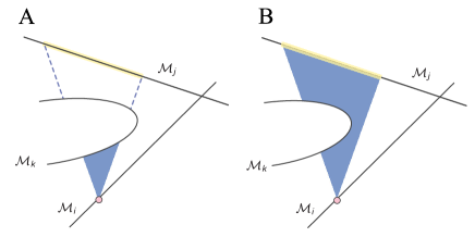
Figure 1: An illustrative example of the stoichiometric rays overestimate the controllable set. (A) All the paths from the pink point are blocked by the null-reaction manifold ${\mathcal{M}}_{k}$. However, Def.2 judges that there are rays from the pink point to the highlighted region on ${\mathcal{M}}_{j}$. (B) An example case where a part of the single stoichiometric rays are blocked, but the stoichiometric rays correctly judge the reachability.

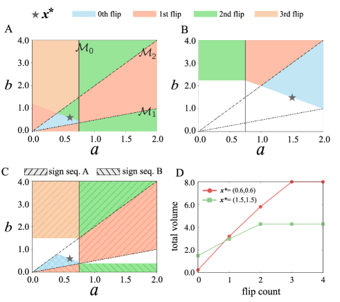
Figure 2: The stoichiometric rays of the reversible Brusselator model. The null-reaction manifold $\mathcal{M}_{0},\mathcal{M}_{1},$ and $\mathcal{M}_{2}$ are represented by the solid, dash, and dot-dash lines, respectively. The phase space is restricted to $[0,2]\times[0,4]$ for computation. (A) The stoichiometric rays of $\bm{x}^{*}=(0.6,0.6)$. The regions covered for the first time at each flip are filled with different colors. The whole region is covered within $3$ flips. (B) The stoichiometric rays of $\bm{x}^{*}=(1.5,1.5)$. In this case, the bottom left region is never covered even if we allow arbitrarily larger flips. (C) The unions of all single stoichiometric rays of $\bm{x}^{*}=(0.6,0.6)$ with two example sign sequences are depicted. The sign sequence A and B follow are $(1,-1,-1)\to(-1,-1,-1)\to(-1,-1,1)\to(1,-1,1)$ and $(1,-1,-1)\to(1,1,-1)\to(-1,1,-1)$, respectively. (D) The total volume of the union of the rays is plotted against the flip count. $\bm{k}=(0.75,2.0,2.0)$ is used.

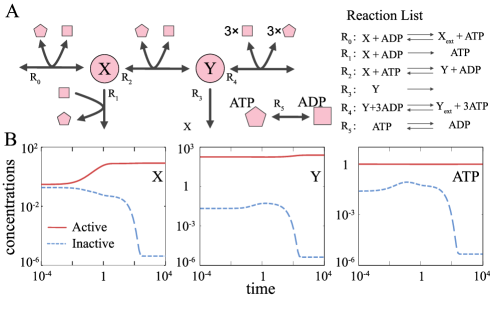
Figure 3: (A) A schematic of the reaction network. The list of the reactions is shown on the right side of the diagram. (B) Example dynamics of metabolites X, Y, and ATP converging to the active (red), and inactive attractors (blue), respectively. Parameters are set to $\bm{u}=(1.0,10.0,1.0,0.1,1.0,0.01)$ and $\bm{k}=(10.0,0.0,0.1,10^{-5},1.0,0.0)$.

The reversible Brusselator is a nonlinear model with linear thermodynamic parts. Next, let us deal with a nonlinear model with a nonlinear thermodynamic part. Here we consider a toy model of metabolism consisting of the metabolites X, Y, ATP, and ADP (a network schematic and the reaction list are shown in Fig.3 A).

The rate equation is given by

$$\derivative{t}\begin{pmatrix}x\\ y\\ z\\ w\end{pmatrix}=\mathbb{S}\bigl{(}\bm{u}\odot\bm{f}(\bm{x})\odot\bm{p}(\bm{x})\bigr{)}$$

$$= \begin{pmatrix}-1&-1&-1&0&0&0\\ 0&0&1&-1&-1&0\\ -1&-1&-1&0&3&-1\\ 1&1&1&0&-3&1\end{pmatrix}\begin{pmatrix}u_{0}\\ u_{1}\\ u_{2}\\ u_{3}\\ u_{4}\\ u_{5}\end{pmatrix}\odot\begin{pmatrix}xw-k_{0}z\\ xw-k_{1}z\\ xz-k_{2}yw\\ y-k_{3}\\ yw-k_{4}z\\ z-k_{5}w\end{pmatrix},$$

where $x,y,z,$ and $w$ represent the concentration of metabolite X, Y, ATP, and ADP, respectively. In the second line of the above equation, $\bm{f}(\bm{x})=\bm{1}$ is omitted. As the total concentration of ATP and ADP is a conserved quantity in the model, we replace $w$ by $z_{\rm tot}-z$ where $z_{\rm tot}$ is the total concentration of the two (we set $z_{\rm tot}$ to be unity in the following).

As shown in Fig. 3B, the model exhibits bistablity with a given, constant $\bm{u}$. On one attractor (the endpoint of the red line), X molecules taken up from the environment are converted into Y and secreted to the external environment with the net production of a single ATP molecule per single X molecule. On the other hand at the other attractor (the endpoint of the blue line), almost all X molecules taken up are secreted to the external environment via the reaction ${\rm R}_{1}$. Y is also taken up from the external environment while consuming 3ATPs. Note that the reaction ${\rm R}_{0}$ consumes a single ATP molecule to uptake a single X molecule, and the reaction ${\rm R}_{1}$ produces a single ATP molecule. For the model to obtain a net gain of ATP, it needs to convert X into Y by consuming one more ATP via reaction ${\rm R}_{2}$. However, once the model falls into the attractor where ATP is depleted (the endpoint of the blue line of Fig. 3B), it can invest no more ATP via ${\rm R}_{2}$, and the model is “dead-locked” by the state. Hereafter, we refer to the former and the latter attractors as the active attractor $\bm{x}^{A}$ and inactive attractor $\bm{x}^{I}$, respectively.

Now, let us ask whether the inactive attractor is a returnable state to the active attractor by controlling the enzyme activities, or it is a “dead” state that cannot be escaped from no matter how the enzyme activities are controlled. To this end, we compute the complement set of the stoichiometric paths of the active attractor, $\mathcal{D}(\bm{x}^{A})=\mathbb{R}_{>0}^{N}\backslash{\rm SP}(\bm{x}^{A})$. We call this complement set the non-returnable set to the active attractor. If the inactive attractor is contained in this set, the inactive attractor is a “dead” state.

Due to the challenges associated with computing the stoichiometric paths, we utilize the stoichiometric rays for the computation. Let us term $\tilde{\mathcal{D}}(\bm{x}^{A})=\mathbb{R}_{>0}^{N}\backslash{\rm SR}(\bm{x}^{A})$ as the narrowed non-returnable set. As the stoichiometric rays is a superset of the stoichiometric paths, the narrowed non-returnable set is a subset of the non-returnable set. Note that, thus the stoichiometric rays does not show a false negative of returnability; If $\bm{x}\in\tilde{\mathcal{D}}(\bm{x}^{A})$ holds, then $\bm{x}$ is guaranteed to be non-returnable to the active attractor.

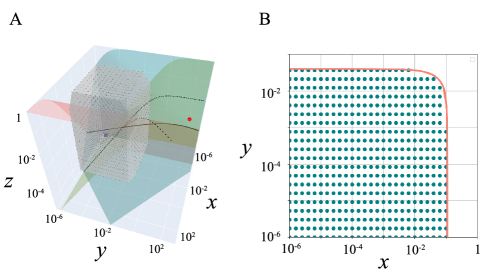
Figure 4: (A) The active attractor (red point), the inactive attractor (blue box), and the points in the narrowed non-returnable set (black dots) are plotted. The point inside the gray rectangle is the convex hull of the non-returnable points judged by the stoichiometric rays. The null-reaction manifolds $\mathcal{M}_{0}$, $\mathcal{M}_{2}$, and $\mathcal{M}_{4}$ are drawn as the salmon, green-blue, and olive-colored surfaces. The null-reaction manifold $\mathcal{M}_{5}$ is not illustrated because it is not necessary for the argument. The intersections of the null-manifold pairs $(\mathcal{M}_{0}$, $\mathcal{M}_{2})$, $(\mathcal{M}_{2}$, $\mathcal{M}_{4})$, and $(\mathcal{M}_{4}$, $\mathcal{M}_{0})$ are represented by the solid, dash, and dot-dash curves, respectively. (B) An analytic estimate of the boundary of the narrowed non-returnable set (red curve) and the points of the narrowed non-returnable set (green-blue points) are plotted. $\log_{10}z$ value is fixed to $-1.7$. We set $L=4$. The same $\bm{k}$ values with Fig.3 are used.

In Fig. 4A, the narrowed non-returnable set of the active attractor with a finite $L$, $\tilde{\mathcal{D}}_{L}(\bm{x}^{A})=\mathbb{R}_{>0}^{N}\backslash{\rm SR}_{L}(\bm{x}^{A})$ is depicted in the phase space (For the computational procedure, see SI text section S3 and SI Codes). The points inside the narrowed non-returnable set cannot return to the active attractor regardless of how the model is controlled with a given number of possible flips. The inactive attractor is contained in the narrowed non-returnable set, and thus, the state, once falls into the inactive attractor, never returns to the active attractor, i.e, the model “dies”. Also, the boundary of the narrowed non-returnable set now gives the life-death boundary of the model.

In Fig. 4B, we plot the points of the narrowed non-returnable set with an analytically estimated life-death boundary of the set on the 2-dimensional slice of the phase space where $z$ value is set to a single value. The boundary is calculated from the thermodynamic and stoichiometric constraints that each single stoichiometric ray should satisfy. The curves match well with the boundary of the narrowed non-returnable set (for the detailed calculation, see SI Text section S4).

Another application of the stoichiometric rays is revealing the structural constraint on the bifurcations of the model. As a demonstration, we sampled several points in the phase space (Fig.5A) and computed the controllability for all the pairs of the sample points. If $\bm{x}\in{\rm SR}_{L}(\bm{y})$ holds, we add a directed edge $\bm{x}\to\bm{y}$ to construct the transition diagram among the points. For ease of visualization, we grouped the points by the strongly connected components (SCCs) of the constructed diagram and drew the component graph where each SCC is a single node (Fig.5B). Note that the bottomest SCC, $C^{*}$, has only in-edges. This means that the points in $C^{*}$ cannot escape from the set, regardless of the control $\bm{u}(t)$.

This constrains the possible bifurcation in the model. By setting the control parameters constant, $\bm{u}(t)=\bm{u}_{\rm cst}$, we obtain the autonomous version of Eq.(4). Let $\bm{\xi}(t;\bm{x},\bm{u}_{\rm cst})$ denotes the solution of the model Eq.(4) with the parameter $\bm{u}_{\rm cst}$ and with the initial point $\bm{x}$. Since the points in $C^{*}$ cannot escape from the set, all such trajectories stay in $C^{*}$, i.e., $\bm{\xi}(t;\bm{x},\bm{u}_{\rm cst})\in C^{*}$ holds for ${}^{\forall}t\geq 0,\bm{x}\in C^{*}$, and $\bm{u}_{\rm cst}\in\mathbb{R}_{\geq 0}^{R}$. In this model, $C^{*}$ is a bounded set, and thus, at least one attractor must be in $C^{*}$. This attractor corresponds to the inactive attractor with the parameter choice used to generate Fig.3B.

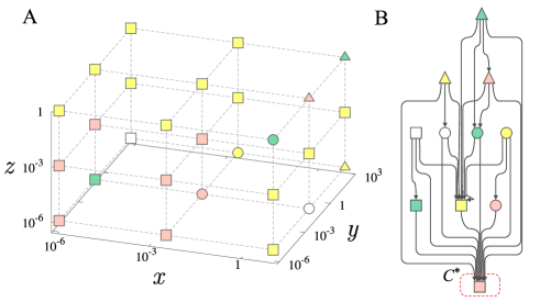
Figure 5: The transition diagram of the discrete states of the toy metabolic model. (A) The points for which the mutual transitivity is computed. The points are grouped and labeled by the strongly connected components (SCCs). The dashed lines are eye guides. (B) The transition diagram of the SCCs. Only the two SCCs (pink- and yellow squares) contain more than one state. The bottom SCC (pink square, indicated by the red-dashed rectangle), $C^{*}$, has only in-edges. The same $\bm{k}$ values with Fig.3 are used, and $L=4$.

In the present letter, we introduced the stoichiometric rays as a tool to compute the controllable set with the enzymatic activity (or the reaction rate constant) as the control parameter. The heart of the stoichiometric rays is that the modulation of the enzymatic activity cannot directly change the directionalities of the reactions. Thus, the partition of the phase space into direction subsets is invariant to the enzymatic activities which allows us to efficient computations of the stoichiometric rays. The usefulness of the stoichiometric rays was demonstrated by using two simple nonlinear models of chemical reactions. Especially, in the second example, we showed that the stoichiometric rays is a powerful tool to compute the non-returnable set in which no control can return the state back to the active attractor with a given number of flips.

Determining the returnability of the state is crucial in understanding biological irreversibility, especially cell death. There are several criteria for the death of microbial cells. A straightforward criterion is checking the growth rate at a given time point. However, the doubling time of several microbes in the deep sea are estimated up to a million years [14]. Viability check by the dead cell staining such as propidium iodide is a common method, but it is not always reliable [15] especially if the lipid membrane is intact. The regrow experiment is a direct check of the viability, but it is repeatedly reported that cells can show a long lag time before the regrowth [16, 17], and there is no guiding principle for how long we should wait for the regrowth. The stoichiometric rays can provide a quantitative criterion for the death of in silico cells. Although it is not directly applicable to the experimental systems, we can quantify the “life-death boundary”, or rather, we like to borrow a word from Buddhism and call it Sanzu Hypersurface , of in silico cells using the stoichiometric rays, and it may contribute to the development of a new criterion for cell death based on the intracellular states and mathematical theory of “death”.

The thermodynamic (ir)reversibility is believed to be a key to grasping the biological (ir)reversibility such as the irreversibility of some diseases and death. However, there is no system-level link between thermodynamic and biological reversibilities except few cases where the simple causality leads to biological irreversibility such as transmissible spongiform encephalopathy [18]. The stoichiometric rays enables us to bridge the (ir)reversibility of each reaction to the system-level reversibility; Recall that the boundary of the non-returnable set is calculated from the thermodynamic constraint, i.e., directionality of the reactions, and the stoichiometric constraint. Further studies should pave the way to unveil the relationship between thermodynamic irreversibility and biological irreversibility. This may reveal the energy (or “negentropy” [19]) needed to maintain cellular states away from the life-death boundary or the Sanzu Hypersurface [20].

We thank Chikara Furusawa for the discussions. This work is supported by JSPS KAKENHI (Grant Numbers JP22K15069, JP22H05403 to Y.H.; 19H05799 to T.J.K.), JST (Grant Numbers JPMJCR2011, JPMJCR1927 to T.J.K.), and GteX Program Japan Grant Number JPMJGX23B4. S.A.H. is financially supported by the JSPS Research Fellowship Grant No. JP21J21415.

References

- [1] Richard Wolfenden and Mark J Snider. The depth of chemical time and the power of enzymes as catalysts. Accounts of chemical research, 34(12):938–945, 2001.
- [2] Oliver Kotte, Judith B Zaugg, and Matthias Heinemann. Bacterial adaptation through distributed sensing of metabolic fluxes. Mol. Syst. Biol., 6:355, March 2010.
- [3] George Stephanopoulos, Aristos A Aristidou, and Jens Nielsen. Metabolic engineering: principles and methodologies. 1998.
- [4] Frederick C Neidhardt, John L Ingraham, Moselio Schaechter, et al. Physiology of the bacterial cell. 1990.
- [5] B Wayne Bequette. Nonlinear control of chemical processes: a review. Ind. Eng. Chem. Res., 30(7):1391–1413, July 1991.
- [6] C C Pedersen and T W Hoffman. The road to advanced process control: From DDC to Real-Time optimization and beyond. IFAC Proceedings Volumes, 30(9):251–279, June 1997.
- [7] Y Tozawa, S Kawasaki, H Matsuo, M Ogawa, and G Emoto. Production control in ethylene plant. In Proceedings IECON ’91: 1991 International Conference on Industrial Electronics, Control and Instrumentation, pages 938–943 vol.2. IEEE, 1991.
- [8] Stephen H Saperstone. Global controllability of linear systems with positive controls. SIAM J. Control Optim., 11(3):417–423, August 1973.
- [9] Gyula Farkas. Local controllability of reactions. J. Math. Chem., 24(1):1–14, August 1998.
- [10] D Dochain and L Chen. Local observability and controllability of stirred tank reactors. J. Process Control, 2(3):139–144, January 1992.
- [11] Dániel András Drexler and János Tóth. Global controllability of chemical reactions. J. Math. Chem., 54(6):1327–1350, June 2016.
- [12] Martin Feinberg. Foundations of Chemical Reaction Network Theory. Springer, Cham, 2019.
- [13] A. Cornish-Bowden. Fundamentals of Enzyme Kinetics. Wiley, 2013.
- [14] Tori M Hoehler and Bo Barker Jørgensen. Microbial life under extreme energy limitation. Nat. Rev. Microbiol., 11(2):83–94, February 2013.
- [15] Miki Umetani, Miho Fujisawa, Reiko Okura, Takashi Nozoe, Shoichi Suenaga, Hidenori Nakaoka, Edo Kussell, and Yuichi Wakamoto. Observation of non-dormant persister cells reveals diverse modes of survival in antibiotic persistence. October 2021.
- [16] Irit Levin-Reisman, Orit Gefen, Ofer Fridman, Irine Ronin, David Shwa, Hila Sheftel, and Nathalie Q Balaban. Automated imaging with ScanLag reveals previously undetectable bacterial growth phenotypes. Nat. Methods, 7(9):737–739, September 2010.
- [17] Yoav Kaplan, Shaked Reich, Elyaqim Oster, Shani Maoz, Irit Levin-Reisman, Irine Ronin, Orit Gefen, Oded Agam, and Nathalie Q Balaban. Observation of universal ageing dynamics in antibiotic persistence. Nature, 600(7888):290–294, December 2021.
- [18] Steven J Collins, Victoria A Lawson, and Colin L Masters. Transmissible spongiform encephalopathies. The Lancet, 363(9402):51–61, 2004.
- [19] Erwin Schrödinger. What is life? The physical aspect of the living cell and mind. Cambridge university press Cambridge, 1944.
- [20] SJ Pirt. The maintenance energy of bacteria in growing cultures. Proceedings of the Royal Society of London. Series B. Biological Sciences, 163(991):224–231, 1965.