QCD Sum Rule study of $J^{P}=1^{\pm}$ exotic states with two heavy quarks in the molecular picture

Abstract

In this study, the spectroscopic parameters of the exotic molecular states composed of mesons containing two heavy quarks (scalar - axial and pseudoscalar - axial meson combinations) are investigated within QCD sum rules. Our findings reveal that the molecular states containing charm quarks do not form bound states, whereas the states with b-quarks can form the exotic molecular states. This observation has significant implications for understanding the structure of these exotic states.

I Introduction

Numerous exotic hadronic states have been observed [1, 2, 3, 4, 5]. Among these states, the exotic doubly charmed $T_{cc}$ state receives particular interest. This state was observed at LHCb near the $D^{0}D^{\ast+}$ threshold in $D^{0}D^{0}\pi^{+}$ mass distribution with mass difference $\delta m=m_{T_{cc}}-(m_{D^{\ast+}}+m_{D^{0}})=(-273\pm 65\pm 5_{-14}^{+11})~{}\rm{keV}$ and decay width $\Gamma=(410\pm 165\pm 43_{-98}^{+18})~{}\rm{keV}$ [6]. Further analysis reveals that this state has the quantum numbers $J^{P}=1^{+}$. Although, this state had been already predicted theoretically in [7, 8], this was the first observation of tetraquark with doubly charmed quarks. This discovery triggered intensive theoretical studies [3, 4, 5, 6, 7, 8, 9, 10, 11, 12, 13, 14, 15, 16, 17, 18, 19, 20, 21, 22]. See the review articles [23, 24, 25, 26, 27, 28] for further details on the topic.

In addition to the exotic state with doubly $c$-quarks, the quark model also predicts the existence of states with two $bb$ and $bc$ heavy quarks. The states with doubly heavy quarks are usually described as tetraquark or molecular states. In the molecular picture, two quark and two anti-quark can form two color singlet mesons by exchanging light mesons. With this prediction, we can further explore the characteristics of these states. To better understand the characteristics of these states, high-precision experimental data and refined theoretical calculations are needed near $DD^{*}(s)$, $BB^{*}(s)$ thresholds.

In the present work, we study the exotic molecular states composed of scalar - axial mesons as well as pseudoscalar - axial mesons containing two heavy quarks with quantum numbers $J^{P}=1^{\pm}$ in the framework of the QCD sum rules [19]. The paper is organized as follows. In Section II, we calculate the correlation functions of the exotic states with quantum numbers $J^{P}=1^{\pm}$ within the molecular picture and derive the formulas for the mass and residues of these states. Section III presents the numerical analysis of the sum rules obtained for the masses and residues and the final section contains our conclusion.

II Sum rules for the exotic $J^{P}=1^{\pm}$ states in molecular picture

In this section, we derive the mass sum rules for the exotic states with quantum numbers $J^{P}=1^{\pm}$ within the molecular picture. The interpolating current for these states can be written as,

$$j_{\mu}=\left(\bar{Q}_{1}^{a}\Gamma_{1}q^{a}\right)\left(\bar{Q}_{2}^{b}\Gamma_{2\mu}q^{b}\right)~{},$$ (1)

where $q_{1}$, $q_{2}$ and $Q$ represent light $u,d,s$ and heavy $b$ or $c$ quarks, respectively. The sum rules for the interpolating current with $\Gamma_{1}=i\gamma_{5}$ and $\Gamma_{2\mu}=\gamma_{\mu}$ were studied in [11]. However, the interpolating current with $J^{P}=1^{+}$ can also be chosen as $\Gamma_{1}=1$, $\Gamma_{2\mu}=\gamma_{\mu}\gamma_{5}$ and the state with $J^{P}=1^{-}$ can be represented by $\Gamma_{1}=\gamma_{5}$, and $\Gamma_{2\mu}=\gamma_{\mu}\gamma_{5}$ or $\Gamma_{1}=1$. These cases are denoted as $\rm{I}$ and $\rm{II}$, respectively. In the present work, we try to answer the following question: if these molecular structures were realized in nature what would be their masses and residues?

In order to determine the mass sum rules, the following correlation function is considered,

$$\Pi_{\mu\nu}^{(i)}\!\!\! = \!\!\!i\int d^{4}x\,e^{ipx}\left<0\left|T\left\{j_{\mu}(x)j_{\nu}^{+}(0)\right\}\right|0\right>~{},$$ (2)

$$= \!\!\!\left(-g_{\mu\nu}+{p_{\mu}p_{\nu}\over p^{2}}\right)\Pi_{1}^{(i)}(p^{2})+{p_{\mu}p_{\nu}\over p^{2}}\Pi_{0}^{(i)}(p^{2})~{},$$

where $i$ corresponds to the relevant currents.

The polarization functions, $\Pi_{0}^{(i)}(p^{2})$ and $\Pi_{1}^{(i)}(p^{2})$ correspond to the spin-0 and spin-1 intermediate states, respectively. In further discussions, we will focus on the structure $-g_{\mu\nu}+\frac{p_{\mu}p_{p}\nu}{p^{2}}$ since it only contains the contribution of the spin-1 particles.

The sum rules for the relevant physical quantity can be obtained by calculating the correlation function in terms of the hadrons and quark-gluon degrees of freedom in the deep Euclidean region $p^{2}\to-\infty$ by using the operator product expansion (OPE). Then, by matching both representations and performing Borel transformation over the variable $-p^{2}$, the desired sum rules are obtained.

At the hadronic level, the correlation function can be calculated with the help of the dispersion relation for the invariant function $\Pi_{1}^{(i)}$,

$$\Pi_{1}^{(i)}={(p^{2})^{\alpha}\over\pi}\int_{(2m_{Q}+m_{q_{1}}+m_{q_{2}})^{2}}^{\infty}{{\rm Im}\Pi_{1}^{(i)}(s)\over(s^{2})^{\alpha}(s-p^{2}-i\epsilon)}+\mbox{\rm subtraction terms}~{}.$$ (3)

In the sum rules method, ${\rm Im}\Pi_{1}^{(i)}(s)$ is defined as the spectral density function,

$$\rho^{(i)}(s)={1\over\pi}{\rm Im}\Pi_{1}^{(i)}=\lambda_{i}^{2}\delta(s-m_{i}^{2})+\mbox{\rm continuum + higher states contributions}~{},$$ (4)

where $m_{i}$ is the lowest-lying resonance. The decay constant $\lambda_{i}$ is defined in the standard way as,

$$\left<0\left|j_{\mu}^{(i)}\right|T_{QQ}(p)\right>=\lambda_{i}\epsilon_{\mu}~{},$$ (5)

with the polarization vector $\epsilon_{\mu}$ of $J^{P}=1^{-}(1^{+})$ states. Using Eq. (4), we obtain the following expression for the correlation function from hadronic side for the structure $\left(-g_{\mu\nu}+{p_{\mu}p_{\nu}\over p^{2}}\right)$,

$$\Pi_{1}^{(i)}={\lambda_{i}^{2}\over m_{i}^{2}-p^{2}}~{}.$$ (6)

Moreover, the correlation function $\Pi_{1}^{(i)}$ can be calculated from the QCD side with the help of the OPE in deep Euclidean domain $p^{2}\to-\infty$ and we get,

$$\Pi_{\mu\nu}\!\!\! = \!\!\!i\int d^{4}x\,e^{ipx}\Big{\{}{\rm Tr}\Big{[}\Gamma_{1}S_{Q}^{aa_{1}}(x)\widetilde{\Gamma}_{1}S_{q_{1}}^{a_{1}a}(-x)\Big{]}\times{\rm Tr}\Big{[}\Gamma_{2}S_{Q}^{bb_{1}}(x)\widetilde{\Gamma}_{2}S_{q_{2}}^{b_{1}b}(-x)\Big{]}$$ (7)

$$- \!\!\!{\rm Tr}\Big{[}S_{Q}^{ba_{1}}(x)\widetilde{\Gamma}_{1}S_{q_{1}}^{a_{1}a}(-x)\Gamma_{1}S_{Q}^{ab_{1}}(x)\widetilde{\Gamma}_{2}S_{q_{2}}^{b_{1}b}(-x)\Gamma_{2}\Big{]}~{},$$

in terms of the light $S_{q_{i}}$ and heavy $S_{Q}$ quark propagators. Hence, to calculate the correlation function from the QCD side, we need the explicit expressions of the light and heavy quark propagators.

The light quark propagator in $x$-representation, up to linear order in light quark mass is given as,

$$S_{q}^{ab}(x)\!\!\! = \!\!\!{i\hbox to0.0pt{/\hss}{x}\over 2\pi^{2}x^{4}}\delta^{ab}-{m_{q}\over 4\pi^{2}x^{2}}\delta^{ab}-{\langle\bar{q}q\rangle\over 12}\left(1-i{m_{q}\over 4}\hbox to0.0pt{/\hss}{x}\right)\delta^{ab}-{x^{2}\over 192}m_{0}^{2}\langle\bar{q}q\rangle\left(1-i{m_{q}\over 6}\hbox to0.0pt{/\hss}{x}\right)\delta^{ab}$$ (8)

$$+ \!\!\!{i\over 32\pi^{2}x^{2}}g_{s}G_{\mu\nu}^{ab}(\sigma^{\mu\nu}\hbox to0.0pt{/\hss}{x}+\hbox to0.0pt{/\hss}{x}\sigma^{\mu\nu})-{1\over 3^{3}\,2^{10}}\langle\bar{q}q\rangle\langle g_{s}^{2}G^{2}\rangle x^{4}\delta^{ab}+\cdots,$$

where $\langle\bar{q}q\rangle$ is the light quark condensate, $G_{\mu\nu}$ is the gluon field strange tensor. Besides, the heavy quark propagator in $x$–representation is given as (see for example [11]),

$$S_{Q}(x)^{ab}\!\!\! = \!\!\!{m_{Q}^{2}\delta^{ab}\over(2\pi)^{2}}\left[i\hbox to0.0pt{/\hss}{x}{K_{2}(m_{Q}\sqrt{-x^{2}})\over\ (\sqrt{-x^{2}})^{2}}+{K_{1}(m_{Q}\sqrt{-x^{2}})\over\sqrt{-x^{2}}}\right]$$ (9)

$$- \!\!\!{m_{Q}g_{s}G_{\mu\nu}^{ab}\over 8(2\pi)^{2}}\left[i(\sigma^{\mu\nu}\hbox to0.0pt{/\hss}{x}+\hbox to0.0pt{/\hss}{x}\sigma^{\mu\nu}){K_{1}(m_{Q}\sqrt{-x^{2}})\over\sqrt{-x^{2}}}+2\sigma^{\mu\nu}K_{0}(m_{Q}\sqrt{-x^{2}})\right]$$

$$- \!\!\!{\langle g_{s}^{2}G^{2}\rangle\delta^{ab}\over(3^{2}\,2^{8}\pi)^{2}}\left[(im_{Q}\hbox to0.0pt{/\hss}{x}-6)(-x^{2}){K_{1}(m_{Q}\sqrt{-x^{2}})\over\sqrt{-x^{2}}}+m_{Q}x^{4}{K_{2}(m_{Q}\sqrt{-x^{2}})\over(\sqrt{-x^{2}})^{2}}\right]~{},$$

where $K_{0}$, $K_{1}$ and $K_{2}$ are the modified Bessel functions of the second kind. Using the explicit expressions of the light and heavy quark propagators, we obtain the spectral density $\rho^{(i)}$ after standard but tedious calculations, as given in Appendix A.

By equating the coefficients of the corresponding Lorentz structures of the correlation function from both representations, we obtain the sum rules of the relevant physical quantities. As a final step, to suppress the contributions of higher and continuum, we perform Borel transformation with respect to $-p^{2}$

$$\lambda^{2}e^{-m^{2}/M^{2}}=\int_{s_{min}}^{s_{0}}ds\,e^{-s/M^{2}}\rho(s)~{},$$ (10)

where $s_{0}$ is the continuum threshold, $M^{2}$ is the Borel mass parameter, and $s_{min}=(m_{Q_{1}}+m_{Q_{2}}+m_{q_{1}}+m_{q_{2}})^{2}$. Note that the mass sum rules for $T_{QQ}$ can easily be obtained by taking derivative with respect to inverse Borel mass parameter, from which we get,

$$m^{2}={\int_{s_{min}}^{s_{0}}ds\,se^{-s/M^{2}}\rho(s)\over\int_{s_{min}}^{s_{0}}ds\,e^{-s/M^{2}}\rho(s)}~{}.$$ (11)

Having determined the mass of the considered states, the residues can be found using Eq. 10.

III Numerical Analysis

In this section, we perform numerical analysis on the sum rules for the tetraquark states with doubly heavy quarks with $J^{P}=1^{\pm}$ that we obtained in the previous section. The sum rules contain many input parameters, such as quark and gluon condensates of appropriate dimensions and masses of the quarks. The numerical values of these input parameters are listed in Table 1. For the heavy quark masses, we use their values in the $\overline{MS}$ scheme.

$\Pi_{i}$ Structures $\overline{m}_{s}(2~{}\rm{GeV})$ $93.4^{+8.6}_{-3.4}~{}\rm{MeV}$  [29] $\overline{m}_{b}(\overline{m}_{b})$ $4.18^{+0.03}_{-0.02}~{}\rm{GeV}$  [29] $\overline{m}_{c}(\overline{m}_{c})$ $(1.27\pm 0.02)~{}\rm{GeV}$  [29] $\langle\bar{q}q\rangle~{}\rm{(1~{}GeV)}$ $(-1.65\pm 0.15)\times 10^{-2}~{}\rm{GeV}^{3}$  [30] $\langle\bar{s}s\rangle$ $(0.8\pm 0.2)\langle\bar{q}q\rangle~{}\rm{GeV^{3}}$  [30] $m_{0}^{2}$ $(0.8\pm 0.2)~{}\rm{GeV^{2}}$  [30] $\langle\frac{\alpha_{s}G^{2}}{\pi}\rangle$ $(0.012\pm 0.006)~{}\rm{GeV^{4}}$  [31]

Table 1: The numerical values of the constant parameters used in our calculations are listed.

In addition to these input parameters, the sum rules contain also two auxiliary parameters, namely, Borel mass $M^{2}$ and the continuum threshold $s_{0}$. To decide the working regions of $s_{0}$ and $M^{2}$, it is important to examine how the mass of the tetraquark state will vary with changes in parameter values. The dependency should be minimal. Moreover, following requirements should be met for an acceptable Borel mass parameter region:

• The upper bound of $M^{2}$ is obtained from the requirement that the continuum and higher states contributions constitute a maximum of 40% of the total result, i.e., the pole contribution (PC) should dominate. This is determined by the following ratio,

  $$PC={\int_{s_{min}}^{s_{max}}ds\,\rho(s)e^{-s/M^{2}}\over\int_{s_{min}}^{\infty}ds\,\rho(s)e^{-s/M^{2}}}~{}.$$

• The minimum value of $M^{2}$ is established by the requirement that the OPE should be convergent. We must ensure that any condensate with the highest number of dimensions contributes less than 5% to the total result.

• The continuum threshold parameter $s_{0}$ can be determined by requiring that the dependency of the mass of the considered state exhibit minimum variation for the Borel mass window that satisfies the conditions mentioned above.

To ensure that all the requirements are met, numerical analysis are performed. And the working regions of the parameters $M^{2}$ and $s_{0}$ are identified which are presented in Table 2.

$M^{2}~{}(\rm{GeV^{2}})$ $s_{0}~{}(\rm{GeV^{2}})$ $J^{P}=1^{-}(\rm{I})$ $BB_{1}$ $9-12$ $130\pm 2$ $BB_{1s}$ $9-12$ $132\pm 2$ $B_{s}B_{1}$ $9-12$ $132\pm 2$ $B_{s}B_{1s}$ $9-12$ $134\pm 2$ $J^{P}=1^{-}(\rm{II})$ $B_{0}B^{*}$ $9-12$ $130\pm 2$ $B_{0}B^{*}_{s}$ $9-12$ $132\pm 2$ $B_{0s}B^{*}$ $9-12$ $132\pm 2$ $B_{0s}B^{*}_{s}$ $9-12$ $134\pm 2$ $J^{P}=1^{+}$ $B_{0}B_{1}$ $9-12$ $134\pm 2$ $B_{0}B_{1s}$ $9-12$ $136\pm 2$ $B_{0s}B_{1}$ $9-12$ $136\pm 2$ $B_{0s}B_{1s}$ $9-12$ $140\pm 2$

Table 2: The working regions of $M^{2}$ and $s_{0}$ for the considered molecular states.

As an example, Figs. 1 and 2 show the dependency of the masses and residues of $BB_{1}$ and $B_{0}B_{1}$ states on $M^{2}$, at the fixed values of $s_{0}$ for $J^{P}=1^{-}$ and $J^{P}=1^{+}$ states, respectively. These figures indicate that when $M^{2}$ varies in the domain $10~{}\rm{GeV^{2}}\leq M^{2}\leq 12~{}\rm{GeV^{2}}$ (after $M^{2}=12~{}\rm{GeV^{2}}$ the results practically do not change) the masses of the $BB_{1}$ and $B_{0}B_{1}$ states exhibit quite good stability.

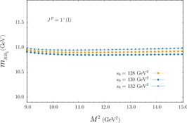
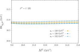
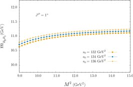
Figure 1: Dependence of the mass of the $BB_{1}$ $B_{0}B^{*}$, and $B_{0}B_{1}$ molecular states on $M^{2}$ at fixed values of the continuum threshold $s_{0}$

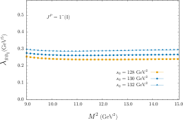
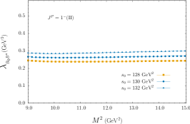
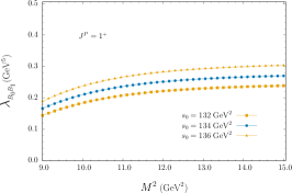
Figure 2: Dependence of the residue of the $BB_{1}$, $B_{0}B^{*}$, and $B_{0}B_{1}$ molecular states on $M^{2}$ at fixed values of the continuum threshold $s_{0}$

Performing similar analysis, we obtained the masses and the residues of the other possible molecular states, the results of which are given in Table 3.

		MASS $\rm{(GeV)}$	RESIDUE $\rm{(GeV^{5})}$
$J^{P}=1^{-}(\rm{I})$	$BB_{1}$	$10.90\pm 0.03$	$0.26\pm 0.02$
	$BB_{1s}$	$10.94\pm 0.03$	$0.27\pm 0.04$
	$B_{s}B_{1}$	$10.94\pm 0.03$	$0.27\pm 0.04$
	$B_{s}B_{1s}$	$11.10\pm 0.02$	$0.30\pm 0.02$
$J^{P}=1^{-}(\rm{II})$	$B_{0}B^{*}$	$10.92\pm 0.03$	$0.27\pm 0.02$
	$B_{s}B^{*}_{s}$	$10.94\pm 0.03$	$0.28\pm 0.02$
	$B_{0s}B^{*}$	$10.96\pm 0.03$	$0.28\pm 0.02$
	$B_{0s}B^{*}_{s}$	$11.10\pm 0.04$	$0.32\pm 0.02$
$J^{P}=1^{+}$	$B_{0}B_{1}$	$11.00\pm 0.10$	$0.20\pm 0.02$
	$B_{0}B_{1s}$	$11.15\pm 0.05$	$0.24\pm 0.03$
	$B_{0s}B_{1}$	$11.15\pm 0.05$	$0.24\pm 0.03$
	$B_{0s}B_{1}$	$11.25\pm 0.05$	$0.28\pm 0.02$

Table 3: Numerical results for the masses and residues of the $B_{(s)}B_{1(s)}$ and $B_{0(s)}B_{1(s)}$ molecular systems

Similar analysis are also performed for doubly charmed systems. Our numerical calculations show that for the Borel Mass parameter region in which the pole contribution is greater than $1/2$, we can not find the stable plateau for the mass of the doubly charmed states. Therefore, we infer that mesons containing two charm quarks do not form bound states in molecular picture considered. This phenomenon has also been noted in several works [32, 33, 34, 35, 36, 37]. The large difference in QQ binding energy for the c and b quarks can explain this outcome. It should be noted that the doubly charmed tetraquark states with $J^{P}=1^{+}$ (scalar-axial current) was considered in [9] with slightly different current and they predicted the mass of these states on the contrary to our result. The main difference is that in [9], the input parameters of the QCD parameters are used at a different $\mu$ scale, however, in our case traditional $\mu=1~{}\rm{GeV}$ scale is used. These studies can be very helpful in putting together the pieces of the puzzle concerning the composition of these tetraquark states.

For a final remark, we would like to note that the intermediate two meson states can also contribute to the correlation functions under consideration. However, it is shown in [38, 39] that the contributions to the correlation functions coming from these two meson states are quite small, and therefore can safely be neglected. For this reason, these contributions are not taken into account in this study.

Conclusion

In this work, we study the spectroscopic parameters, namely masses and residues of the potential exotic states with the quantum numbers $J^{P}=1^{\pm}$, containing two heavy quarks in the molecular picture within QCD sum rule. Our findings revealed that no bound states can be formed for the $T_{cc}$ states with quantum numbers $J^{P}=1^{\pm}$ for the considered currents. On the other hand, for the $T_{bb}$ states, our calculations demonstrated that bound states can indeed exist within both considered molecular frameworks. This result significantly contributes to the ongoing discussions in the literature regarding the inner nature of exotic states. Furthermore, the obtained mass values for $J^{P}=1^{+}$ and $J^{P}=1^{-}$ exotic states within the molecular picture show a difference of $\sim 200~{}\rm{MeV}$. This result can be checked in future experiments to establish the ”right” picture.

Even though it is challenging to determine the states near $BB^{*}(s)$ and $DD^{*}(s)$ thresholds, the results obtained for the masses of the tetraquark states can be considered in future experiments looking for exotic hadrons.

Appendix A

In this Appendix, we present the expressions of the spectral density $\rho(s)$ for the $J^{P}=1^{-}(\rm{I})$, $J^{P}=1^{-}(\rm{II})$, and $J^{P}=1^{+}$ tetraquark systems. Upper (lower) sign corresponds to $1^{-}(\rm{I})$ $(1^{+})$ quantum number. With the replacement of $m_{u}\to-m_{u}$ and $\langle\bar{u}u\rangle=-\langle\bar{u}u\rangle$ for the $J^{P}=1^{-}(\rm{I})$ case, one can obtain the spectral density for the $J^{P}=1^{-}(\rm{II})$ case.

$$\rho^{(pert)}(s)\!\!\! = \!\!\!\pm{1\over(3\times 2^{14})\pi^{6}}\int_{\alpha_{min}}^{\alpha_{max}}{d\alpha\over\alpha^{3}}\int_{\beta_{min}}^{\beta_{max}}{d\beta\over\beta^{3}}\Big{[}(\alpha+\beta)m_{b}^{2}-\alpha\beta s\Big{]}^{2}$$

$$\times \!\!\!\Big{\{}(1-\beta)\beta m_{b}^{3}\Big{(}[8+29\beta(1+\beta)]m_{b}\mp 120\beta[(1+\beta)m_{d}\mp 2m_{u})\Big{)}$$

$$- \!\!\!\alpha^{4}(29m_{b}^{2}-33\beta s)(m_{b}^{2}-\beta s)+2\alpha m_{b}\big{\{}m_{b}\big{[}(4+21\beta-58\beta^{3})m_{b}^{2}$$

$$\mp \!\!\!12\beta(33-32\beta)m_{d}m_{u}\mp 60\beta m_{b}(m_{d}-3\beta^{2}m_{d}\mp 2m_{u}\pm 4\beta m_{u})\big{]}$$

$$- \!\!\!(1-\beta)\beta\big{[}(4+31\beta(1+\beta))m_{b}\mp 60\beta(m_{d}+\beta m_{d}\mp 2m_{u})\big{]}s\big{\}}$$

$$- \!\!\!2\alpha^{3}\beta(58m_{b}^{4}\mp 60m_{b}^{3}m_{d}-93\beta m_{b}^{2}s\pm 60\beta m_{b}m_{d}s+33\beta^{2}s^{2})$$

$$+ \!\!\!3\alpha^{2}\big{\{}(7-58\beta^{2})m_{b}^{4}+40\beta m_{b}^{3}(\pm 3\beta m_{d}-2m_{u})\mp 80\beta^{2}m_{b}(\beta m_{d}\mp m_{u})s$$

$$\pm \!\!\!2\beta m_{b}^{2}(128m_{d}m_{u}\mp 9s\pm 31\beta^{2}s)+\beta^{2}s\big{[}\pm 8m_{d}m_{u}+11(1-\beta^{2})s\big{]}\big{\}}\Big{\}}$$

$$\rho^{(\langle\bar{d}d\rangle\langle\bar{u}u\rangle)}(s)\!\!\! = \!\!\!-{\langle\bar{d}d\rangle\langle\bar{u}u\rangle\over(3\times 2^{8})\pi^{2}}\int_{\alpha_{min}}^{\alpha_{max}}d\alpha\Big{\{}4m_{b}\big{[}13m_{b}-5(\pm 2m_{d}-m_{u})\big{]}$$

$$+ \!\!\!\alpha\big{[}12m_{0}^{2}+8m_{b}(m_{b}\pm 5m_{d})-m_{u}(20m_{b}\pm 33m_{d})-12s\big{]}$$

$$- \!\!\!3\alpha^{2}(4m_{0}^{2}\mp 11m_{d}m_{u}-4s)\Big{\}}$$

$$\rho^{(m_{0}^{2}\langle\bar{d}d\rangle\langle g^{2}G^{2}\rangle)}(s)\!\!\! = \!\!\!{5(m_{0}^{2}\langle\bar{d}d\rangle\langle g^{2}G^{2}\rangle)\over(3\times 2^{12})m_{b}\pi^{4}}\int_{\alpha_{min}}^{\alpha_{max}}d\alpha(1-\alpha)^{2}$$

$$\rho^{(m_{0}^{2}\langle\bar{u}u\rangle\langle g^{2}G^{2}\rangle)}(s)\!\!\! = \!\!\!\mp{5(m_{0}^{2}\langle\bar{u}u\rangle\langle g^{2}G^{2}\rangle)\over(3\times 2^{11})m_{b}\pi^{4}}\int_{\alpha_{min}}^{\alpha_{max}}d\alpha(1-\alpha)^{2}$$

$$\rho^{(m_{0}^{2}\langle\bar{d}d\rangle)}(s)\!\!\! = \!\!\!\mp{m_{0}^{2}\langle\bar{d}d\rangle\over(3\times 2^{10})\pi^{4}}\int_{\alpha_{min}}^{\alpha_{max}}{d\alpha\over\alpha}\Big{\{}m_{b}\big{[}\pm 30m_{b}^{2}-20m_{d}m_{u}(1-\alpha)\alpha$$

$$- \!\!\!\alpha m_{b}(12m_{d}+22\alpha m_{d}\mp 39m_{u}\mp 6\alpha m_{u})\big{]}$$

$$- \!\!\!(1-\alpha)\alpha(\pm 30m_{b}-22\alpha m_{d}\pm 9\alpha m_{u})s\Big{\}}$$

$$+ \!\!\!{m_{0}^{2}\langle\bar{d}d\rangle\over(3\times 2^{10})\pi^{4}}\int_{\alpha_{min}}^{\alpha_{max}}{d\alpha\over\alpha}\int_{\beta_{min}}^{\beta_{max}}d\beta\Big{\{}m_{b}^{2}\big{[}30(\alpha+\beta)m_{b}\mp\alpha m_{d}\big{]}-30m_{b}\alpha\beta s\Big{\}}$$

$$\rho^{(m_{0}^{2}\langle\bar{u}u\rangle)}(s)\!\!\! = \!\!\!\pm{m_{0}^{2}\langle\bar{u}u\rangle\over(3\times 2^{10})\pi^{4}}\int_{\alpha_{min}}^{\alpha_{max}}{d\alpha\over\alpha}\Big{\{}m_{b}\big{[}30m_{b}^{2}\mp 10m_{d}m_{u}(1-\alpha)\alpha$$

$$+ \!\!\!\alpha m_{b}(12m_{u}+22\alpha m_{u}\mp 39m_{d}\mp 6\alpha m_{d})\big{]}$$

$$- \!\!\!(1-\alpha)\alpha(30m_{b}\mp 9\alpha m_{d}+22\alpha m_{u})s\Big{\}}$$

$$\mp \!\!\!{m_{b}^{2}m_{u}m_{0}^{2}\langle\bar{u}u\rangle\over(3\times 2^{10})\pi^{4}}\int_{\alpha_{min}}^{\alpha_{max}}d\alpha\int_{\beta_{min}}^{\beta_{max}}d\beta$$

$$\rho^{(\langle\bar{d}d\rangle\langle g^{2}G^{2}\rangle)}(s)\!\!\! = \!\!\!-{\langle\bar{d}d\rangle\langle g^{2}G^{2}\rangle\over(3^{2}\times 2^{13})m_{b}\pi^{4}}\int_{\alpha_{min}}^{\alpha_{max}}{d\alpha\over\alpha}\Big{\{}4\big{[}3-\alpha(193-15\alpha)\big{]}m_{b}^{2}$$

$$+ \!\!\!\alpha m_{b}\big{[}(\pm 763\mp 760\alpha)m_{d}-2(61+74\alpha+6\alpha^{2})m_{u}\big{]}$$

$$\pm \!\!\!40(1-\alpha)\alpha\big{[}3(1-\alpha)m_{d}m_{u}+(\pm 3\mp 2\alpha)s\big{]}\Big{\}}$$

$$+ \!\!\!{\langle\bar{d}d\rangle\langle g^{2}G^{2}\rangle\over(3^{2}\times 2^{13})m_{b}\pi^{4}}\int_{\alpha_{min}}^{\alpha_{max}}{d\alpha\over\alpha}\int_{\beta_{min}}^{\beta_{max}}d\beta\Big{\{}4\big{[}8\alpha-9(3+2\beta)\big{]}m_{b}^{2}$$

$$\pm \!\!\!3\alpha m_{b}m_{d}+120\alpha\beta s\Big{\}}$$

$$\rho^{(\langle\bar{u}u\rangle\langle g^{2}G^{2}\rangle)}(s)\!\!\! = \!\!\!-{\langle\bar{u}u\rangle\langle g^{2}G^{2}\rangle\over(3^{2}\times 2^{13})m_{b}\pi^{4}}\int_{\alpha_{min}}^{\alpha_{max}}{d\alpha\over\alpha}\Big{\{}\pm 4\big{[}21+2\alpha(17-5\alpha)\big{]}m_{b}^{2}$$

$$- \!\!\!\alpha m_{b}\big{[}2(61+74\alpha+6\alpha^{2})m_{d}\mp(133-130\alpha)m_{u}\big{]}$$

$$- \!\!\!60(1-\alpha)^{2}\alpha(m_{d}m_{u}\pm 2s)\Big{\}}$$

$$\pm \!\!\!{\langle\bar{u}u\rangle\langle g^{2}G^{2}\rangle\over(3\times 2^{13})\pi^{4}}\int_{\alpha_{min}}^{\alpha_{max}}{d\alpha\over\alpha}\int_{\beta_{min}}^{\beta_{max}}d\beta(12m_{b}+\alpha m_{u})$$

$$\rho^{(\langle g^{2}G^{2}\rangle^{2})}(s)\!\!\! = \!\!\!\mp{\langle g^{2}G^{2}\rangle^{2}\over(3^{3}\times 2^{18})m_{b}^{2}\pi^{6}}\int_{\alpha_{min}}^{\alpha_{max}}{d\alpha\over\alpha}\Big{\{}\big{[}192-\alpha(4143+584\alpha)\big{]}m_{b}^{2}$$

$$\mp \!\!\!132\alpha\big{[}1-2(3-\alpha)\alpha\big{]}m_{d}m_{u}\pm 20\alpha m_{b}\big{[}(31+74\alpha)m_{d}\mp 11(m_{u}+2\alpha m_{u})\big{]}$$

$$- \!\!\!8(3-\alpha)(1-\alpha)\alpha s\Big{\}}$$

$$+ \!\!\!{\langle g^{2}G^{2}\rangle^{2}\over(3^{3}\times 2^{17})m_{b}^{2}\pi^{6}}\int_{\alpha_{min}}^{\alpha_{max}}{d\alpha\over\alpha}\int_{\beta_{min}}^{\beta_{max}}{d\beta\over\beta}\Big{\{}(\pm)m_{b}\big{[}18\alpha^{2}m_{b}+18(22-9\beta)\beta m_{b}$$

$$+ \!\!\!5\alpha\beta(37m_{b}\mp 24m_{d})\big{]}\mp 6\alpha\beta(3\alpha+5\beta)s\Big{\}}$$

$$\rho^{(\langle g^{2}G^{2}\rangle)}(s)\!\!\! = \!\!\!\pm{\langle g^{2}G^{2}\rangle\over(3\times 2^{15})m_{b}\pi^{6}}\int_{\alpha_{min}}^{\alpha_{max}}{d\alpha\over\alpha(1-\alpha)}\Big{\{}\big{[}m_{b}^{2}-(1-\alpha)\alpha s\big{]}$$

$$\times \!\!\!\Big{(}m_{b}\big{[}33m_{b}^{2}\mp 80(1-\alpha)m_{d}m_{u}-20m_{b}(m_{d}\mp m_{u})\big{]}$$

$$- \!\!\!(1-\alpha)\alpha\big{[}33m_{b}\mp 20(m_{d}\mp m_{u})\big{]}s\Big{)}\Big{\}}$$

$$- \!\!\!{\langle g^{2}G^{2}\rangle\over(3\times 2^{16})m_{b}\pi^{6}}\int_{\alpha_{min}}^{\alpha_{max}}{d\alpha\over\alpha^{2}}\int_{\beta_{min}}^{\beta_{max}}{d\beta\over\beta^{2}}\Bigg{\{}\pm\beta m_{b}^{4}\Big{(}\big{\{}108+\beta\big{[}219+\beta(360+233\beta)\big{]}\big{\}}m_{b}$$

$$+ \!\!\!24\beta\big{\{}\big{[}6+4(1-\beta)\beta\big{]}m_{d}\mp(3-5\beta)m_{u}\big{\}}\Big{)}$$

$$\mp \!\!\!3\alpha^{4}m_{b}(m_{b}^{2}-\beta s)^{2}\pm 2\alpha^{3}(m_{b}^{2}-\beta s)\big{\{}2m_{b}^{2}\big{[}(27+47\beta)m_{b}\pm 18\beta m_{d}\big{]}$$

$$\mp \!\!\!\beta^{2}(\pm 61m_{b}-80m_{d})s\big{\}}$$

$$+ \!\!\!2m_{b}^{2}\alpha\Big{(}m_{b}\Big{[}\pm 3\big{\{}18+\beta\big{[}1+2\beta(82+55\beta)\big{]}\big{\}}m_{b}^{2}-6\beta(12+35\beta)m_{d}m_{u}$$

$$+ \!\!\!4\beta m_{b}\big{\{}3\big{[}6-5\beta(14+\beta)\big{]}m_{d}\mp(9-94\beta)m_{u}\big{\}}\Big{]}$$

$$\mp \!\!\!\beta\Big{[}\big{\{}54+\beta\big{[}111+5\beta(114+37\beta)\big{]}\big{\}}m_{b}$$

$$- \!\!\!12\beta\big{\{}\big{[}6+\beta(4-9\beta)\big{]}m_{d}\mp(3-10\beta)m_{u}\big{\}}\Big{]}s\Big{)}$$

$$- \!\!\!\alpha^{2}\Big{[}m_{b}^{3}\Big{(}(\pm)3(71-244\beta-206\beta^{2})m_{b}^{2}+8\beta m_{b}\big{[}6(37-\beta)m_{d}\mp 79m_{u}\big{]}+420\beta m_{d}m_{u}\Big{)}$$

$$\pm \!\!\!2\beta m_{b}\Big{(}m_{b}\big{\{}\big{[}105-\beta(702+343\beta)\big{]}m_{b}\pm 8\beta(111+19\beta)m_{d}\big{\}}$$

$$- \!\!\!94\beta(4m_{b}\mp 3m_{d})m_{u}\Big{)}s\pm\beta^{2}\big{\{}\big{[}3+\beta(780+137\beta)\big{]}m_{b}-120\beta(\pm\beta m_{d}-m_{u})\big{\}}s^{2}\Big{]}\Bigg{\}}$$

$$\rho^{(\langle\bar{d}d\rangle)}(s)\!\!\! = \!\!\!\mp{\langle\bar{d}d\rangle\over 2^{10}\pi^{4}}\int_{\alpha_{min}}^{\alpha_{max}}{d\alpha\over\alpha(1-\alpha)}\big{[}m_{b}^{2}-(1-\alpha)\alpha s\big{]}\Big{\{}m_{b}\big{\{}11m_{b}m_{d}$$

$$\mp \!\!\!2\big{[}m_{b}\mp 10(1-\alpha)m_{d}\big{]}m_{u}\big{\}}-(1-\alpha)\alpha(11m_{d}\mp 2m_{u})s\Big{\}}$$

$$- \!\!\!{\langle\bar{d}d\rangle\over 2^{10}\pi^{4}}\int_{\alpha_{min}}^{\alpha_{max}}{d\alpha\over\alpha^{2}}\int_{\beta_{min}}^{\beta_{max}}{d\beta\over\beta}\big{[}(\alpha+\beta)m_{b}^{2}-\alpha\beta s\big{]}\Big{\{}m_{b}^{2}\big{\{}(\alpha+\beta)$$

$$\times \!\!\!\big{[}20(\alpha+\beta)m_{b}\pm 9\alpha m_{d}\big{]}+44\alpha m_{u}\big{\}}\mp\alpha\beta\big{[}(\pm)20(\alpha+\beta)m_{b}+11\alpha m_{d}\big{]}s\Big{\}}$$

$$\rho^{(\langle\bar{u}u\rangle)}(s)\!\!\! = \!\!\!-{\langle\bar{u}u\rangle\over 2^{10}\pi^{4}}\int_{\alpha_{min}}^{\alpha_{max}}{d\alpha\over\alpha(1-\alpha)}\big{[}m_{b}^{2}-(1-\alpha)\alpha s\big{]}$$

$$\times \!\!\!\big{[}20(1-\alpha)m_{b}m_{d}m_{u}+m_{b}^{2}(2m_{d}\mp 11m_{u})-(1-\alpha)\alpha(2m_{d}\mp 11m_{u})s\big{]}$$

$$\pm \!\!\!{\langle\bar{u}u\rangle\over 2^{10}\pi^{4}}\int_{\alpha_{min}}^{\alpha_{max}}{d\alpha\over\alpha^{2}}\int_{\beta_{min}}^{\beta_{max}}{d\beta\over\beta}\big{[}(\alpha+\beta)m_{b}^{2}-\alpha\beta s\big{]}$$

$$\times \!\!\!\Big{\{}m_{b}\big{\{}\pm 4m_{b}\big{[}\pm 5(\alpha+\beta)m_{b}-11\alpha m_{d}\big{]}-\alpha\big{[}9(\alpha+\beta)m_{b}\mp 20\beta m_{d}\big{]}m_{u}\big{\}}$$

$$- \!\!\!\alpha\beta(20m_{b}-11\alpha m_{u})s\Big{\}}$$

$$\alpha_{min}\!\!\! = \!\!\!{s-\sqrt{s(s-4m_{b}^{2})}\over 2s}~{},$$

$$\alpha_{max}\!\!\! = \!\!\!{s+\sqrt{s(s-4m_{b}^{2})}\over 2s}~{},$$

$$\beta_{min}\!\!\! = \!\!\!{m_{b}^{2}\alpha\over s\alpha-m_{b}^{2}}~{},$$

$$\beta_{max}\!\!\! = \!\!\!1-\alpha~{}.$$

The results for the spectral densities containing strange quarks can also be obtained from the presented results by replacing the mass(es) and condensate(s) of the appropriate light quark(s) with those of the s-quark.