Multi-Derivative Runge-Kutta Flux Reconstruction for hyperbolic conservation laws

Arpit Babbar Centre for Applicable Mathematics Tata Institute of Fundamental Research Bangalore – 560065 arpit@tifrbng.res.in &Praveen Chandrashekar Centre for Applicable Mathematics Tata Institute of Fundamental Research Bangalore – 560065 praveen@math.tifrbng.res.in Corresponding author 0000-0002-9453-370X 0000-0003-1903-4107

(March 4, 2024)

Abstract

We extend the fourth order, two stage Multi-Derivative Runge Kutta (MDRK) scheme of Li and Du to the Flux Reconstruction (FR) framework by writing both of the stages in terms of a time averaged flux and then use the approximate Lax-Wendroff procedure. Numerical flux is computed in each stage using D2 dissipation and EA flux, enhancing Fourier CFL stability and accuracy respectively. A subcell based blending limiter is developed for the MDRK scheme which ensures that the limited scheme is provably admissibility preserving. Along with being admissibility preserving, the blending scheme is constructed to minimize dissipation errors by using Gauss-Legendre solution points and performing MUSCL-Hancock reconstruction on subcells. The accuracy enhancement of the blending scheme is numerically verified on compressible Euler’s equations, with test cases involving shocks and small-scale structures.

1 Introduction

The idea to apply Multiderivative Runge-Kutta Flux Reconstruction on the time dependent conservation law

$$\bm{u}_{t}+\bm{f}\left(\bm{u}\right)_{x}=\bm{0}$$

is to cast the fourth order multi-derivative Runge-Kutta scheme of [18] in the form of

$$\begin{split}\bm{u}^{\ast}&=\bm{u}^{n}-\Delta t\partial_{x}\bm{F}^{\ast}\\ \bm{u}^{n+1}&=\bm{u}^{n}-\Delta t\partial_{x}\bm{F}\end{split}$$

where

$$\partial_{x}\bm{F}^{\ast}=\partial_{x}\bm{F}^{\ast}\left(\bm{u}^{n}\right)\approx\partial_{x}\int_{t^{n}}^{t^{n+1/2}}\bm{f}\text{\text{{{d}}}}t,\qquad\partial_{x}\bm{F}=\partial_{x}\bm{F}\left(\bm{u}^{n},\bm{u}^{\ast}\right)\approx\partial_{x}\int_{t^{n}}^{t^{n+1}}\bm{f}\text{\text{{{d}}}}t$$

The method is two-stage; in the first stage, $\bm{F}^{\ast}$ is locally approximated and then Flux Reconstruction (FR) [16] is used to construct a globally continuous approximation of $\bm{F}^{\ast}$ which is used to perform evolution to $\bm{u}^{\ast}~{}\eqref{eq:intro.us.evolution}$; and the same procedure is then performed using $\bm{F}$ for evolution to $\bm{u}^{n+1}$.

1.1 Motivation and literature review

Higher order methods incorporate higher order terms and perform more computations per degree of freedom, increasing accuracy and arithmetic intensity, and making these methods relevant to the current state of memory-bound HPC hardware [1, 31]. Spectral element methods like Discontinuous Galerkin (DG) and Flux Reconstruction (FR) are two high order methods that are suitable for modern requirements due to their parallelization, capability of handling curved meshes and shock capturing.

Discontinuous Galerkin (DG) is a Spectral Element Method first introduced by Reed and Hill [24] for neutron transport equations and developed for fluid dynamics equations by Cockburn and Shu and others, see [9] and the references therein. The DG method uses an approximate solution which is a polynomial within each element and is allowed to be discontinuous across interfaces. The neighbouring DG elements are coupled only through the numerical flux and thus bulk of computations are local to the element, minimizing data transfers.

Flux Reconstruction (FR) is also a class of discontinuous Spectral Element Methods introduced by Huynh [16] and uses the same solution approximation as DG. FR method is obtained by using the numerical flux and correction functions to construct a continuous flux approximation and collocating the differential form of the equation. Thus, FR is quadrature free and all local operations can be vectorized. The choice of the correction function affects the accuracy and stability of the method [16, 36, 37, 35]; by properly choosing the correction function and solution points, FR method can be shown to be equivalent to some discontinuous Galerkin and spectral difference schemes [16, 35]. A provably non-linearly stable FR in split form was obtained in [8].

FR and DG are procedures for discretizing the equation in space and can be used to obtain a system of ODEs in time, i.e., a semi-discretization of the PDE. The standard approach to solve the semi-discretization is to use a high order multi-stage Runge-Kutta method. In this approach, the spatial discretization has to be performed in every RK stage and thus the expensive operations of MPI communication and limiting have to be performed multiple times per time step.

An alternative approach is to use high order single-stage solvers, which include ADER schemes [34, 11] and Lax-Wendroff schemes [22, 21, 42, 6, 7]; see [3, 4] for a more in-depth review.

Lax-Wendroff schemes perform a Taylor’s expansion in time to the order of the desired accuracy and compute the temporal derivatives locally. Multiderivative Runge-Kutta (MDRK) scheme also make use of temporal derivatives but they combine them with multiple stages to obtain the desired order of accuracy. As MDRK schemes use both temporal derivatives and multiple stages, they are a generalization of LW and standard multistage RK methods [26]. MDRK methods typically require fewer temporal derivatives in contrast to the Lax-Wendroff schemes and fewer stages in contrast to the standard RK methods, which is what makes them promising.

Multiderivative Runge-Kutta (MDRK) [19] methods were initially developed to solve systems of ODE like

$$\frac{\mathrm{d}\bm{u}}{\mathrm{d}t}=\bm{L}\left(\bm{u}\right)$$

that use temporal derivatives of $\bm{L}$, see [26] for a review of MDRK methods for solving ODEs. They were first used for temporal discretization of hyperbolic conservation laws in [26] by using Weighted Essentially Non-Oscillatary (WENO) [29] and Discontinuous Galerkin (DG) [9] methods for spatial discretization.

In [3], a Lax-Wendroff Flux Reconstruction (LWFR) scheme was proposed which used the approximate Lax-Wendroff procedure of [42] to obtain an element local high order approximation of the time averaged flux which was made globally continuous using FR; the globally continuous time averaged flux approximation was used to perform evolution to the next time level. The numerical flux was carefully constructed in [3] to obtain enhanced accuracy and stability. In [4], a subcell based shock capturing blending scheme was introduced for LWFR based on the subcell based scheme of [15]. To enhance accuracy, [4] used Gauss-Legendre solution points and performed MUSCL-Hancock reconstruction on the subcells. Since the subcells used in [4] were inherently non-cell centred, the MUSCL-Hancock scheme was extended to non-cell centred grids along with the proof of [5] for admissibility preservation. The subcell structure was exploited to obtain a provably admissibility preserving LWFR scheme by careful construction of the blended numerical flux at the element interfaces.

In [18], a two stage fourth order MDRK scheme was introduced for solving hyperbolic conservation laws by solving a Generalized Riemann Problem (GRP). In this work, we show the first combination of MDRK with a Flux Reconstruction scheme by using the scheme of [18]. We also use the construction of the numerical flux from [3]. In particular, we use the D2 dissipation introduced in [3] and show that it leads to enhanced Fourier CFL stability limiter. We also use the EA scheme from [3] which leads to enhanced accuracy for non-linear problems when using Gauss-Legendre solution points. We also develop admissibility preserving subcell based blending scheme based on [4] and show how it superior to other schemes like a TVB limiter.

1.2 Outline

The rest of this paper is organized as follows. The discretization of the domain and function approximation by polynomials is presented in Section 2. Section 3 reviews the one dimensional Runge-Kutta Flux Reconstruction (RKFR) method and Section 4 introduces the MDRK method in an FR framework. In particular, Section 4.3 discusses approximate Lax-Wendroff procedure applied to MDRK, Sections 4.4 discuss the D2 dissipation for computing the dissipative part of the numerical flux to enhance Fourier CFL stability limit and Section 4.6 discusses the EA scheme for computing the central part of numerical flux to enhance stability. The Fourier stability analysis is performed in Section 5 to demonstrate the improved stability of D2 dissipation. In Section 6, we explain the admissibility preserving blending limiter for MDRK scheme. The numerical results validating the order of accuracy and capability of the blending scheme are shown in Section 7 and a summary of the new MDRK scheme is presented in Section 8.

2 conservation law

Consider a conservation law of the form

$$\bm{u}_{t}+\bm{f}(\bm{u})_{x}=\bm{0}$$ (1)

where $\bm{u}\in\mathbb{R}^{p}$ is the vector of conserved quantities, $\bm{f}(\bm{u})$ is the corresponding flux, together with some initial and boundary conditions. The solution that is physically correct is assumed to belong to an admissible set, denoted by $\mathcal{U}_{\textrm{$\operatorname{ad}$}}$. For example in case of compressible flows, the density and pressure (or internal energy) must remain positive. In case of shallow water equations, the water depth must remain positive. In most of the models that are of interest, the admissible set is a convex subset of $\mathbb{R}^{p}$, and can be written as

$$\mathcal{U}_{\textrm{$\operatorname{ad}$}}=\{\bm{u}\in\mathbb{R}^{p}:p_{k}(\bm{u})>0,1\leq k\leq K\}$$ (2)

where each admissibility constraint $p_{k}$ is concave if $p_{j}>0$ for all $j<k$. For Euler’s equations, $K=2$ and $p_{1},p_{2}$ are density, pressure functions respectively; if the density is positive then pressure is a concave function of the conserved variables. We will divide the computational domain $\Omega$ into disjoint elements $\Omega_{e}$, with

$$\Omega_{e}=[x_{e-\frac{1}{2}},x_{e+\frac{1}{2}}]\qquad\operatorname{and}\qquad\Delta x_{e}=x_{e+\frac{1}{2}}-x_{e-\frac{1}{2}}$$

Let us map each element to a reference element, $\Omega_{e}\to[0,1]$, by

$$x\to\xi=\frac{x-x_{e-\frac{1}{2}}}{\Delta x_{e}}$$

Inside each element, we approximate the solution by $\mathbb{P}_{N}$ functions which are degree $N\geq 0$ polynomials.

Remark 1

In this work, we will only be using degree $N=3$ polynomials as the Multiderivative Runge-Kutta discretization that we use [18] is fourth order. However, the description is given for general $N$ for ease of notation.

To construct $\mathbb{P}_{N}$ polynomials, choose $N+1$ distinct nodes

$$0\leq\xi_{0}<\xi_{1}<\cdots<\xi_{N}\leq 1$$

which will be taken to be Gauss-Legendre (GL) or Gauss-Lobatto-Legendre (GLL) nodes, and will also be referred to as solution points. There are associated quadrature weights $w_{j}$ such that the quadrature rule is exact for polynomials of degree up to $2N+1$ for GL points and upto degree $2N-1$ for GLL points. Note that the nodes and weights we use are with respect to the interval $[0,1]$ whereas they are usually defined for the interval $[-1,+1]$. The solution inside an element is given by

$$x\in\Omega_{e}:\qquad u_{h}(\xi,t)=\sum_{p=0}^{N}\bm{u}_{e,p}(t)\ell_{p}(\xi)$$

where each $\ell_{p}$ is a Lagrange polynomial of degree $N$ given by

$$\ell_{q}(\xi)=\prod_{p=0,p\neq q}^{N}\frac{\xi-\xi_{p}}{\xi_{q}-\xi_{p}}\in\mathbb{P}_{N},\qquad\ell_{q}(\xi_{p})=\delta_{pq}$$

Figure (1a) illustrates a piecewise polynomial solution at some time $t_{n}$ with discontinuities at the element boundaries. Note that the coefficients $\bm{u}_{e,p}$ which are the basic unknowns or degrees of freedom (dof), are the solution values at the solution points.

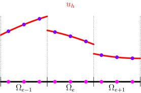
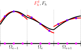
(a)	(b)

Figure 1: (a) Piecewise polynomial solution at time $t_{n}$, and (b) discontinuous and continuous flux.

The numerical method will require spatial derivatives of certain quantities. We can compute the spatial derivatives on the reference interval using a differentiation matrix $\mathsf{D}=[D_{pq}]$ whose entries are given by

$$D_{pq}=\ell_{q}^{\prime}(\xi_{p}),\qquad 0\leq p,q\leq N$$

For example, we can obtain the spatial derivatives of the solution $\bm{u}_{h}$ at all the solution points by a matrix-vector product as follows

$$\left[\begin{array}[]{c}\partial_{x}\bm{u}_{h}(\xi_{0},t)\\ \vdots\\ \partial_{x}\bm{u}_{h}(\xi_{N},t)\end{array}\right]=\frac{1}{\Delta x_{e}}\mathsf{D}\mathsf{u}(t),\qquad\mathsf{u}=\left[\begin{array}[]{c}\bm{u}_{e,0}\\ \vdots\\ \bm{u}_{e,N}\end{array}\right]$$

We will use symbols in sans serif font like $\mathsf{D},\mathsf{u}$, etc. to denote matrices or vectors defined with respect to the solution points. Define the Vandermonde matrices corresponding to the left and right boundaries of a cell by

$$\mathsf{V}_{L}=[\ell_{0}(0),\ell_{1}(0),\ldots,\ell_{N}(0)]^{\top},\qquad\mathsf{V}_{R}=[\ell_{0}(1),\ell_{1}(1),\ldots,\ell_{N}(1)]^{\top}$$ (3)

which is used to extrapolate the solution and/or flux to the cell faces for the computation of inter-cell fluxes.

3 Runge-Kutta FR

The RKFR scheme is based on an FR spatial discretization leading to a system of ODE followed by application of an RK scheme to march forward in time. The key idea is to construct a continuous polynomial approximation of the flux which is then used in a collocation scheme to update the nodal solution values. At some time $t$, we have the piecewise polynomial solution defined inside each cell; the FR scheme can be described by the following steps.

Step 1.

In each element, we construct the flux approximation by interpolating the flux at the solution points leading to a polynomial of degree $N$, given by

$$\bm{f}_{h}^{\delta}(\xi,t)=\sum_{p=0}^{N}\bm{f}(\bm{u}_{e,p}(t))\ell_{p}(\xi)$$

The above flux is in general discontinuous across the elements similar to the red curve in Figure (1b).

Step 2.

We build a continuous flux approximation by adding some correction terms at the element boundaries

$$\bm{f}_{h}(\xi,t)=\left[\bm{f}_{e-\frac{1}{2}}(t)-\bm{f}_{h}^{\delta}(0,t)\right]g_{L}(\xi)+\bm{f}_{h}^{\delta}(\xi,t)+\left[\bm{f}_{e+\frac{1}{2}}(t)-\bm{f}_{h}^{\delta}(1,t)\right]g_{R}(\xi)$$

where

$$\bm{f}_{e+\frac{1}{2}}(t)=\bm{f}(\bm{f}_{h}(x_{e+\frac{1}{2}}^{-},t),\bm{f}_{h}(x_{e+\frac{1}{2}}^{+},t))$$

is a numerical flux function that makes the flux unique across the cells. The continuous flux approximation is illustrated by the black curve in Figure (1b). The functions $g_{L},g_{R}$ are the correction functions which must be chosen to obtain a stable scheme.

Step 3.

We obtain the system of ODE by collocating the PDE at the solution points

$$\frac{\text{\text{{{d}}}}\bm{u}_{p}^{e}}{\text{\text{{{d}}}}t}(t)=-\frac{1}{\Delta x_{e}}\frac{\partial\bm{f}_{h}}{\partial\xi}(\xi_{p},t),\qquad 0\leq p\leq N$$

which is solved in time by a Runge-Kutta scheme.

Correction functions.

The correction functions $g_{L},g_{R}$ should satisfy the end point conditions

$$g_{L}(0)=1,\qquad g_{R}(0)=0$$

$$g_{L}(1)=0,\qquad g_{R}(1)=1$$

which ensures the continuity of the flux, i.e., $\bm{f}_{h}(x_{e+\frac{1}{2}}^{-},t)=\bm{f}_{h}(x_{e+\frac{1}{2}}^{+},t)=\bm{f}_{e+\frac{1}{2}}(t)$. The reader is referred to [3, 16, 36] for discussion and choices of correction functions.

4 Multi-derivative Runge-Kutta FR scheme

The Multi-Derivative Runge-Kutta scheme of [18] will be cast in a Flux Reconstruction framework by writing each stage in terms of a time averaged flux that will be computed with the Approximate Lax-Wendroff procedure [42]. The scheme to solve (1) is thus given by the following two stage procedure

$$\bm{u}^{\ast} =\bm{u}^{n}-\frac{\Delta t}{2}\partial_{x}\bm{F}^{\ast}$$ (4)

$$\bm{u}^{n+1} =\bm{u}^{n}-\Delta t\partial_{x}\bm{F}$$ (5)

where

$$\begin{split}\bm{F}^{\ast}:=&\bm{f}\left(\bm{u}^{n}\right)+\frac{1}{4}\Delta t\frac{\partial}{\partial t}\bm{f}\left(\bm{u}^{n}\right)\\ \bm{F}:=&\bm{f}\left(\bm{u}^{n}\right)+\frac{1}{6}\Delta t\left(\frac{\partial}{\partial t}\bm{f}\left(\bm{u}^{n}\right)+2\frac{\partial}{\partial t}\bm{f}\left(\bm{u}^{\ast}\right)\right)=\frac{1}{\Delta t}\int_{t^{n}}^{t^{n+1}}\bm{f}\left(\bm{u}\right)\text{\text{{{d}}}}t+O(\Delta t^{4})\end{split}$$ (6)

The approximations in (6) ensure that we will get the formal fourth order of accuracy. Then the solution update at the nodes is written as a collocation scheme

$$\begin{split}\bm{u}_{e,p}^{n+1}&=\bm{u}_{e,p}^{n}-\frac{\Delta t}{\Delta x_{e}}\frac{\text{\text{{{d}}}}\bm{F}^{\ast}_{h}}{\text{\text{{{d}}}}\xi}(\xi_{p})\\ \bm{u}_{e,p}^{n+1}&=\bm{u}_{e,p}^{n}-\frac{\Delta t}{\Delta x_{e}}\frac{\text{\text{{{d}}}}\bm{F}_{h}}{\text{\text{{{d}}}}\xi}(\xi_{p})\end{split},\qquad 0\leq p\leq N$$ (7)

where we take $N=3$ to get fourth order accuracy. The major work in the above scheme is involved in the construction of the time average flux approximation $\bm{F}_{h}$ which is explained in subsequent sections.

4.1 Conservation property

The computation of correct weak solutions for non-linear conservation laws in the presence of discontinuous solutions requires the use of conservative numerical schemes. The Lax-Wendroff theorem shows that if a consistent, conservative method converges, then the limit is a weak solution. The method (7) is also conservative though it is not directly apparent; to see this multiply (7) by the quadrature weights associated with the solution points and sum over all the points in the $e^{\operatorname{th}}$ element,

$$\begin{split}\sum_{p=0}^{N}w_{p}\bm{u}_{e,p}^{\ast}&=\sum_{p=0}^{N}w_{p}\bm{u}_{e,p}^{n}-\frac{\Delta t}{\Delta x_{e}}\sum_{p=0}^{N}w_{p}\frac{\partial\bm{F}^{\ast}_{h}}{\partial\xi}(\xi_{p})\\ \sum_{p=0}^{N}w_{p}\bm{u}_{e,p}^{n+1}&=\sum_{p=0}^{N}w_{p}\bm{u}_{e,p}^{n}-\frac{\Delta t}{\Delta x_{e}}\sum_{p=0}^{N}w_{p}\frac{\partial\bm{F}_{h}}{\partial\xi}(\xi_{p})\end{split}$$

The correction functions are of degree $N+1$ and thus the fluxes $\bm{F}^{\ast}_{h},\bm{F}_{h}$ are polynomials of degree $\leq N+1$. If the quadrature is exact for polynomials of degree atleast $N$, which is true for both GLL and GL points, then the quadrature is exact for the flux derivative term and we can write it as an integral, which leads to

$$\begin{split}\int_{\Omega_{e}}\bm{u}^{\ast}_{h}\text{\text{{{d}}}}x&=\int_{\Omega_{e}}\bm{u}_{h}^{n}\text{\text{{{d}}}}x-\Delta t[\bm{F}^{\ast}_{e+\frac{1}{2}}-\bm{F}^{\ast}_{e-\frac{1}{2}}]\\ \int_{\Omega_{e}}\bm{u}^{n+1}_{h}\text{\text{{{d}}}}x&=\int_{\Omega_{e}}\bm{u}_{h}^{n}\text{\text{{{d}}}}x-\Delta t[\bm{F}_{e+\frac{1}{2}}-\bm{F}_{e-\frac{1}{2}}]\end{split}$$ (8)

This shows that the total mass inside the cell changes only due to the boundary fluxes and the scheme is hence conservative. The conservation property is crucial in the proof of admissibility preservation studied in Section 6.3.

Recall that the solutions of conservation law (1) belong to an admissible set $\mathcal{U}_{\textrm{$\operatorname{ad}$}}$ (2). The admissibility preserving property, also known as convex set preservation property (since $\mathcal{U}_{\textrm{$\operatorname{ad}$}}$ is convex) of the conservation law can be written as

$$\bm{u}(\cdot,t_{0})\in\mathcal{U}_{\textrm{$\operatorname{ad}$}}\qquad\Longrightarrow\qquad\bm{u}(\cdot,t)\in\mathcal{U}_{\textrm{$\operatorname{ad}$}},\qquad t>t_{0}$$ (9)

and thus we define an admissibility preserving scheme to be

Definition 1

The flux reconstruction scheme is said to be admissibility preserving if

$$\bm{u}_{e,p}^{n}\in\mathcal{U}_{\textrm{$\operatorname{ad}$}}\quad\forall e,j\qquad\Longrightarrow\qquad\bm{u}_{e,p}^{n+1}\in\mathcal{U}_{\textrm{$\operatorname{ad}$}}\quad\forall e,p$$

where $\mathcal{U}_{\textrm{$\operatorname{ad}$}}$ is the admissibility set of the conservation law.

To obtain an admissibility preserving scheme, we exploit the weaker admissibility preservation in means property defined as

Definition 2

The flux reconstruction scheme is said to be admissibility preserving in the means if

$$\bm{u}_{e,p}^{n}\in\mathcal{U}_{\textrm{$\operatorname{ad}$}}\quad\forall e,p\qquad\Longrightarrow\qquad\overline{\bm{u}}_{e}^{n+1}\in\mathcal{U}_{\textrm{$\operatorname{ad}$}}\quad\forall e$$

where $\mathcal{U}_{\textrm{$\operatorname{ad}$}}$ is the admissibility set of the conservation law.

4.2 Reconstruction of the time average flux

To complete the description of the MDRK method (7), we must explain the method for the computation of the time average fluxes $\bm{F}^{\ast}_{h},\bm{F}_{h}$ when evolving from $t^{n}$ to $t^{n+1}$. In the first stage (4), we compute $\bm{F}^{\ast}_{h}$ which is then used to evolve to $\bm{u}^{\ast}$. In the second stage (5), $\bm{u}^{n},\bm{u}^{\ast}$ are used to compute $\bm{F}_{h}$ which is used from evolution to $\bm{u}^{n+1}$. Since the reconstruction procedure is same for both of the time average fluxes, we explain the procedure of Flux Reconstruction of $\bm{F}_{h}(\xi)$, which is a time averaged flux over the interval $[t^{n},t^{n+1}]$, performed in three steps. Note that all results in this work use degree $N=3$, although the following steps are written for general $N$.

Step 1.

Use the approximate Lax-Wendroff procedure of [42] to compute the time average flux $\bm{F}$ at all the solution points

$$\bm{F}_{p}^{e}\approx\bm{F}(\xi_{p}),\qquad 0\leq p\leq N$$

The approximate LW procedure is the subsection Section 4.3.

Step 2.

Build a local approximation of the time average flux inside each element by interpolating at the solution points

$$\bm{F}_{h}^{\delta}(\xi)=\sum_{j=0}^{N}\bm{F}_{j}^{e}\ell_{p}(\xi)$$

which however may not be continuous across the elements. This is illustrated in Figure (1b).

Step 3.

Modify the flux approximation $\bm{F}_{h}^{\delta}(\xi)$ so that it becomes continuous across the elements. Let $\bm{F}_{e+\frac{1}{2}}$ be some numerical flux function that approximates the flux $\bm{F}$ at $x=x_{e+\frac{1}{2}}$. Then the continuous flux approximation is given by

$$\bm{F}_{h}(\xi)=\left[\bm{F}_{e-\frac{1}{2}}-\bm{F}_{h}^{\delta}(0)\right]g_{L}(\xi)+\bm{F}_{h}^{\delta}(\xi)+\left[\bm{F}_{e+\frac{1}{2}}-\bm{F}_{h}^{\delta}(1)\right]g_{R}(\xi)$$

which is illustrated in Figure 1b. The correction functions $g_{L},g_{R}\in\mathbb{P}_{N+1}$ are chosen from the FR literature [16, 36].

Step 4.

The derivatives of the continuous flux approximation at the solution points can be obtained as

$$\mathsf{\partial_{\xi}F_{h}}=\left[F_{e}-\frac{1}{2}-\mathsf{V}_{L}^{\top}\mathsf{F}\right]\mathsf{b}_{L}+\mathsf{D}\mathsf{F}+\left[F_{e}+\frac{1}{2}-\mathsf{V}_{R}^{\top}\mathsf{F}\right]\mathsf{b}_{R},\qquad\mathsf{b}_{L}=\begin{bmatrix}g_{L}^{\prime}(\xi_{0})\\ \vdots\\ g_{L}^{\prime}(\xi_{N})\end{bmatrix},\qquad\mathsf{b}_{R}=\begin{bmatrix}g_{R}^{\prime}(\xi_{0})\\ \vdots\\ g_{R}^{\prime}(\xi_{N})\end{bmatrix}$$

which can also be written as

$$\mathsf{\partial_{\xi}F_{h}}=\bm{F}_{e-\frac{1}{2}}\mathsf{b}_{L}+\mathsf{D}_{1}\mathsf{F}+\bm{F}_{e+\frac{1}{2}}\mathsf{b}_{R},\qquad\mathsf{D}_{1}=\mathsf{D}-\mathsf{b}_{L}\mathsf{V}_{L}^{\top}-\mathsf{b}_{R}\mathsf{V}_{R}^{\top}$$ (10)

where $\mathsf{V}_{L},\mathsf{V}_{R}$ are Vandermonde matrices which are defined in (3). The quantities $\mathsf{b}_{L},\mathsf{b}_{R},\mathsf{V}_{L},\mathsf{V}_{R},\mathsf{D},\mathsf{D}_{1}$ can be computed once and re-used in all subsequent computations. They do not depend on the element and are computed on the reference element. Equation (10) contains terms that can be computed inside a single cell (middle term) and those computed at the faces (first and third terms) where it is required to use the data from two adjacent cells. The computation of the flux derivatives can thus be performed by looping over cells and then the faces.

4.3 Approximate Lax-Wendroff procedure

The time average fluxes $\bm{F}^{\ast}_{p},\bm{F}_{p}$ must be computed using (6), which involves temporal derivatives of the flux. A natural approach is to use the PDE and replace time derivatives with spatial derivatives, but this leads to large amount of algebraic computations since we need to evaluate the flux Jacobian and its higher tensor versions. To avoid this process, we follow the ideas in [42, 6] and adopt an approximate Lax-Wendroff procedure. To present this idea in a concise and efficient form, we introduce the notation

$$\bm{u}^{(1)}=\Delta t\partial_{t}\bm{u},\qquad\bm{f}^{(1)}=\Delta t\partial_{t}\bm{f}$$

The time derivatives of the solution are computed using the PDE

$$\bm{u}^{(1)}=-\Delta t\partial_{x}\bm{f}$$

The approximate Lax-Wendroff procedure is applied in each element and so for simplicity of notation, we do not show the element index in the following.

First stage

$$\bm{F}^{\ast}:=\bm{f}\left(\bm{u}^{n}\right)+\frac{1}{4}\Delta t\frac{\partial}{\partial t}\bm{f}\left(\bm{u}^{n}\right)=\frac{1}{\Delta t/2}\int_{t^{n}}^{t^{n+1/2}}\bm{f}\left(\bm{u}\right)\text{\text{{{d}}}}t$$ (11)

To obtain fourth order accuracy, the approximation for $\frac{\partial}{\partial t}\bm{f}\left(\bm{u}^{n}\right)$ needs to be third order accurate (Section A) which we obtain as

$$\begin{split}\bm{f}_{t}(\xi,t)&\approx\frac{-\bm{f}(\bm{u}(\xi,t+2\Delta t))+8\bm{f}(\bm{u}(\xi,t+\Delta t))-8\bm{f}(\bm{u}(\xi,t-\Delta t))+\bm{f}(\bm{u}(\xi,t-2\Delta t))}{12\Delta t}\\ &\approx\left.\frac{-\bm{f}(\bm{u}+2\Delta t\bm{u}_{t})+8\bm{f}(\bm{u}+\Delta t\bm{u}_{t})-8\bm{f}(\bm{u}-\Delta t\bm{u}_{t})+\bm{f}(\bm{u}-2\Delta t\bm{u}_{t})}{12\Delta t}\right|_{(\xi,t)}\end{split}$$

Thus, the time averaged flux is computed as

$$\mathsf{F}^{\ast}=\mathsf{f}+\frac{1}{4}\mathsf{f}^{(1)}$$

where

$$\mathsf{u}^{(1)} =-\frac{\Delta t}{\Delta x_{e}}\mathsf{D}\mathsf{f}$$

$$\mathsf{f}^{(1)} =\frac{1}{12}\left[-\bm{f}\left(\mathsf{u}+2\mathsf{u}^{(1)}\right)+8\bm{f}\left(\mathsf{u}+\mathsf{u}^{(1)}\right)-8\bm{f}\left(\mathsf{u}-\mathsf{u}^{(1)}\right)+\bm{f}\left(\mathsf{u}-2\mathsf{u}^{(1)}\right)\right]$$

Second stage.

The time averaged flux is computed as

$$\mathsf{F}=\mathsf{f}+\frac{1}{6}\left(\mathsf{f}^{(1)}+2\text{{\hskip 1.00006pt}f*{\hskip 1.49994pt}}^{(1)}\right)$$

where

$$\text{{\hskip 1.00006pt}u*{\hskip 1.49994pt}}^{(1)} =-\frac{\Delta t}{\Delta x_{e}}\mathsf{D}\text{{\hskip 1.00006pt}f*{\hskip 1.49994pt}}$$

$$\text{{\hskip 1.00006pt}f*{\hskip 1.49994pt}}^{(1)} =\frac{1}{12}\left[-\bm{f}\left(\text{{\hskip 1.00006pt}u*{\hskip 1.49994pt}}+2\text{{\hskip 1.00006pt}u*{\hskip 1.49994pt}}^{(1)}\right)+8\bm{f}\left(\text{{\hskip 1.00006pt}u*{\hskip 1.49994pt}}+\text{{\hskip 1.00006pt}u*{\hskip 1.49994pt}}^{(1)}\right)-8\bm{f}\left(\text{{\hskip 1.00006pt}u*{\hskip 1.49994pt}}-\text{{\hskip 1.00006pt}u*{\hskip 1.49994pt}}^{(1)}\right)+\bm{f}\left(\text{{\hskip 1.00006pt}u*{\hskip 1.49994pt}}-2\text{{\hskip 1.00006pt}u*{\hskip 1.49994pt}}^{(1)}\right)\right]$$

Remark 2

The $\mathsf{f},\mathsf{f}^{(1)}$ computed in the first stage are reused in the second.

4.4 Numerical flux

The numerical flux couples the solution between two neighbouring cells in a discontinuous Galerkin type method. In RK methods, the numerical flux is a function of the trace values of the solution at the faces. In the MDRK scheme, we have constructed time average fluxes at all the solution points inside the element and we want to use this information to compute the time averaged numerical flux at the element faces. The simplest numerical flux is based on Lax-Friedrich type approximation and is similar to the one used for LW [21] and is similar to the D1 dissipation of [3]

$$\begin{split}\bm{F}_{e+\frac{1}{2}}&=\frac{1}{2}[\bm{F}_{e+\frac{1}{2}}^{\ast-}+\bm{F}_{e+\frac{1}{2}}^{\ast+}]-\frac{1}{2}\lambda_{e+\frac{1}{2}}[\bm{u}_{h}(x_{e+\frac{1}{2}}^{+},t_{n})-\bm{u}_{h}(x_{e+\frac{1}{2}}^{-},t_{n})]\\ \bm{F}_{e+\frac{1}{2}}&=\frac{1}{2}[\bm{F}_{e+\frac{1}{2}}^{-}+\bm{F}_{e+\frac{1}{2}}^{+}]-\frac{1}{2}\lambda_{e+\frac{1}{2}}[\bm{u}_{h}(x_{e+\frac{1}{2}}^{+},t_{n})-\bm{u}_{h}(x_{e+\frac{1}{2}}^{-},t_{n})]\end{split}$$ (12)

which consists of a central flux and a dissipative part. For linear advection equation $\bm{u}_{t}+a\bm{u}_{x}=\bm{0}$, the coefficient in the dissipative part of the flux is taken as $\lambda_{e+\frac{1}{2}}=|a|$, while for a non-linear PDE like Burger’s equation, we take it to be

$$\lambda_{e+\frac{1}{2}}=\max\{|\bm{f}^{\prime}(\overline{\bm{u}}_{e}^{n})|,|\bm{f}^{\prime}(\overline{\bm{u}}_{e+1}^{n})|\}$$

where $\overline{\bm{u}}_{e}^{n}$ is the cell average solution in element $\Omega_{e}$ at time $t_{n}$, and will be referred to as Rusanov or local Lax-Friedrich [25] approximation. Note that the dissipation term in the above numerical flux is evaluated at time $t_{n}$ whereas the central part of the flux uses the time average flux. Since the dissipation term contains solution difference at faces, we still expect to obtain optimal convergence rates, which is verified in numerical experiments. This numerical flux depends on the following quantities: $\{\overline{\bm{u}}_{e}^{n},\overline{\bm{u}}_{e+1}^{n},\bm{u}_{h}(x_{e+\frac{1}{2}}^{-},t_{n}),\bm{u}_{h}(x_{e+\frac{1}{2}}^{+},t_{n}),\bm{F}_{e+\frac{1}{2}}^{-},\bm{F}_{e+\frac{1}{2}}^{+}\}$.

The numerical flux of the form (12) leads to somewhat reduced CFL numbers as is experimentally verified and discussed in Section 5, and also does not have upwind property even for linear advection equation. An alternate form of the numerical flux is obtained by evaluating the dissipation term using the time average solution, leading to the formula similar to D2 dissipation of [3]

$$\begin{split}\bm{F}_{e+\frac{1}{2}}^{\ast}&=\frac{1}{2}[\bm{F}_{e+\frac{1}{2}}^{\ast-}+\bm{F}_{e+\frac{1}{2}}^{\ast+}]-\frac{1}{2}\lambda_{e+\frac{1}{2}}[\bm{U}_{e+\frac{1}{2}}^{\ast+}-\bm{U}_{e+\frac{1}{2}}^{\ast-}]\\ \bm{F}_{e+\frac{1}{2}}&=\frac{1}{2}[\bm{F}_{e+\frac{1}{2}}^{-}+\bm{F}_{e+\frac{1}{2}}^{+}]-\frac{1}{2}\lambda_{e+\frac{1}{2}}[\bm{U}_{e+\frac{1}{2}}^{+}-\bm{U}_{e+\frac{1}{2}}^{-}]\end{split}$$ (13)

where

$$\begin{split}\bm{U}^{\ast}&=\mathsf{u}+\frac{1}{4}\mathsf{u}^{(1)}\\ \bm{U}&=\mathsf{u}+\frac{1}{6}\left(\mathsf{u}^{(1)}+2\text{{\hskip 1.00006pt}u*{\hskip 1.49994pt}}^{(1)}\right)\end{split}$$ (14)

are the time average solutions. In this case, the numerical flux depends on the following quantities: $\{\overline{\bm{u}}_{e}^{n},\overline{\bm{u}}_{e+1}^{n},\bm{U}_{e+\frac{1}{2}}^{-},\bm{U}_{e+\frac{1}{2}}^{+},\bm{F}_{e+\frac{1}{2}}^{-},\bm{F}_{e+\frac{1}{2}}^{+}\}$. Following [3], we will refer to the above two forms of dissipation as D1 and D2, respectively. The dissipation model D2 is not computationally expensive compared to the D1 model since all the quantities required to compute the time average solution $\bm{U}$ are available during the Lax-Wendroff procedure. It remains to explain how to compute $\bm{F}_{e+\frac{1}{2}}^{\pm}$ appearing in the central part of the numerical flux. There were two ways introduced for Lax-Wendroff in [3] to compute the central flux, termed AE and EA. We explain how the two apply to MDRK in the next two subsections.

4.5 Numerical flux – average and extrapolate to face (AE)

In each element, the time average flux $\bm{F}_{h}^{\delta}$ corresponding to each stage has been constructed using the Lax-Wendroff procedure. The simplest approximation that can be used for $\bm{F}_{e+\frac{1}{2}}^{\pm}$ in the central part of the numerical flux is to extrapolate the flux $\bm{F}_{h}^{\delta}$ to the faces

$$\bm{F}_{e+\frac{1}{2}}^{\pm}=\bm{F}_{h}^{\delta}(x_{e+\frac{1}{2}}^{\pm})$$

As in [3], we will refer to this approach with the abbreviation AE. However, as shown in the numerical results, this approximation can lead to sub-optimal convergence rates for some non-linear problems. Hence we propose another method for the computation of the inter-cell flux which overcomes this problem as explained next.

4.6 Numerical flux – extrapolate to face and average (EA)

Instead of extrapolating the time average flux from the solution points to the faces, we can instead build the time average flux at the faces directly using the approximate Lax-Wendroff procedure that is used at the solution points. The flux at the faces is constructed after the solution is evolved at all the solution points. In the following equations, $\alpha$ denotes either the left face ($L$) or the right face ($R$) of a cell. For $\alpha\in\{L,R\}$, we compute the time average flux at the faces of the $e$^th element by the following steps, where we suppress the element index since all the operations are performed inside one element.

Stage 1

$$\bm{u}_{\alpha}^{\pm} =\mathsf{V}_{\alpha}^{\top}\left(\mathsf{u}\pm\mathsf{u}^{(1)}\right)$$

$$\bm{f}^{(1)}_{\alpha} =\frac{1}{12}\left[-\bm{f}\left(\bm{u}^{+2}_{\alpha}\right)+8\bm{f}\left(\bm{u}^{+}_{\alpha}\right)-8\bm{f}\left(\bm{u}^{-}_{\alpha}\right)+\bm{f}\left(\bm{u}^{-2}_{\alpha}\right)\right]$$

$$\bm{F}_{\alpha}^{\ast} =\bm{f}(\bm{u}_{\alpha})+\frac{1}{4}\bm{f}^{(1)}_{\alpha}$$

Stage 2

$$\bm{u}_{\alpha}^{\ast\pm} =\mathsf{V}_{\alpha}^{\top}\left(\text{{\hskip 1.00006pt}u*{\hskip 1.49994pt}}\pm\text{{\hskip 1.00006pt}u*{\hskip 1.49994pt}}^{(1)}\right)$$

$$\bm{u}_{\alpha}^{\ast\pm 2} =\mathsf{V}_{\alpha}^{\top}\left(\text{{\hskip 1.00006pt}u*{\hskip 1.49994pt}}\pm 2\text{{\hskip 1.00006pt}u*{\hskip 1.49994pt}}^{(1)}\right)$$

$$\bm{f}^{\ast(1)}_{\alpha} =\frac{1}{12}\left[-\bm{f}\left(\bm{u}^{\ast+2}_{\alpha}\right)+8\bm{f}\left(\bm{u}^{\ast+}_{\alpha}\right)-8\bm{f}\left(\bm{u}^{\ast-}_{\alpha}\right)+\bm{f}\left(\bm{u}^{\ast-2}_{\alpha}\right)\right]$$

$$\bm{F}_{\alpha} =\bm{f}(\bm{u}_{\alpha})+\frac{1}{6}\left(\bm{f}^{(1)}_{\alpha}+2\bm{f}^{\ast(1)}\right)$$

Remark 3

The $\bm{f}(\bm{u}_{\alpha})$, $\bm{f}^{(1)}_{\alpha}$ computed in the first stage are reused in the second stage.

We see that the solution is first extrapolated to the cell faces and the same finite difference formulae for the time derivatives of the flux which are used at the solution points, are also used at the faces. The numerical flux is computed using the time average flux built as above at the faces; the central part of the flux $\bm{F}_{e+\frac{1}{2}}^{\pm}$ in equations (12), (13) are computed as

$$\bm{F}_{e+\frac{1}{2}}^{-}=(\bm{F}_{R})_{e},\qquad\bm{F}_{e+\frac{1}{2}}^{+}=(\bm{F}_{L})_{e+1}$$

We will refer to this method with the abbreviation EA. The dissipative part of the flux is computed using either the solution at time $t_{n}$ or the time average solution, which are extrapolated to the faces, leading to the D1 and D2 models, respectively.

Remark 4

The two methods AE and EA are different only when there are no solution points at the faces. E.g., if we use GLL solution points, then the two methods yield the same result since there is no interpolation error. For the constant coefficient advection equation, the above two schemes for the numerical flux lead to the same approximation but they differ in case of variable coefficient advection problems and when the flux is non-linear with respect to $u$. The effect of this non-linearity and the performance of the two methods are shown later using some numerical experiments.

5 Fourier stability analysis

We now perform Fourier stability analysis of the MDRK scheme applied to the linear advection equation $u_{t}+au_{x}=0$ where $a$ is the constant advection speed. We will assume that the advection speed $a$ is positive and denote the CFL number by

$$\sigma=\frac{a\Delta t}{\Delta x}$$

We will perform the CFL stability analysis for the MDRK scheme with D2 dissipation flux (13) and thus will like to write the two stage scheme as

$$\mathsf{u}_{e}^{n+1}=-\sigma^{2}\mathsf{A}_{-2}\mathsf{u}_{e-2}-\sigma\mathsf{A}_{-1}\mathsf{u}_{e-1}^{n}+\left(1-\sigma\mathsf{A}_{0}\right)\mathsf{u}_{e}^{n}-\sigma\mathsf{A}_{+1}\mathsf{u}_{e+1}^{n}-\sigma^{2}\mathsf{A}_{+2}\mathsf{u}_{e+2}^{n}$$ (15)

where the matrices $\mathsf{A}_{-2},\mathsf{A}_{-1},\mathsf{A}_{0},\mathsf{A}_{+1},\mathsf{A}_{+2}$ depend on the choice of the dissipation model in the numerical flux. We will perform the final evolution by studying both the stages.

5.1 Stage 1

We will try to write the first stage as

$$\mathsf{u}_{e}^{\ast}=-\sigma\mathsf{A}^{\ast}_{-1}\mathsf{u}_{e-1}^{n}+\left(1-\sigma\mathsf{A}_{0}^{\ast}\right)\mathsf{u}_{e}^{n}-\sigma\mathsf{A}_{+1}^{\ast}\mathsf{u}_{e+1}^{n}$$ (16)

Since $f_{t}=au_{t}$, the time average flux for first stage at all solution points is given by

$$\mathsf{F}_{e}^{\ast}=a\mathsf{U}_{e}^{\ast}\quad\operatorname{where}\quad\mathsf{U}_{e}^{\ast}=\mathsf{T}^{\ast}\mathsf{u}_{e}\quad\operatorname{and}\quad\mathsf{T}^{\ast}=\mathsf{I}-\frac{\sigma}{4}\mathsf{D}$$

The extrapolation to the cell boundaries are given by

$$F_{h}^{\ast,\delta}(x_{e-\frac{1}{2}}^{+})=\text{{{V}}}_{L}^{T}\mathsf{F}_{e}^{\ast},\qquad F_{h}^{\ast,\delta}(x_{e+\frac{1}{2}}^{+})=\mathsf{V}_{R}^{T}\mathsf{F}_{e}^{\ast}$$

The D2 dissipation numerical flux is given by

$$\mathsf{F}_{e+\frac{1}{2}}^{\ast}=\mathsf{V}_{R}^{T}\mathsf{F}_{e}^{\ast}=a\mathsf{V}_{R}^{T}\mathsf{T}^{\ast}\mathsf{u}_{e}$$

and the flux differences at the face as

$$F_{e-\frac{1}{2}}^{\ast}-F_{h}^{\ast,\delta}(x_{e-\frac{1}{2}}^{-})=a\mathsf{V}_{R}^{T}\mathsf{u}_{e-1}-a\mathsf{V}_{L}^{T}\mathsf{T}^{\ast}\mathsf{u}_{e},\qquad F_{e+\frac{1}{2}}^{\ast}-F_{h}^{\ast,\delta}(x_{e+\frac{1}{2}}^{-})=0$$

so that the flux derivative at the solution points is given by

$$\partial_{\xi}\mathsf{F}_{h}^{\ast}=\mathsf{b}_{L}\left(a\mathsf{V}_{R}^{T}\mathsf{T}^{\ast}\mathsf{u}_{e-1}-a\mathsf{V}_{L}^{T}\mathsf{T}^{\ast}\mathsf{u}_{e}\right)+a\mathsf{D}\mathsf{T}^{\ast}\mathsf{u}_{e}=a\mathsf{b}_{L}\mathsf{V}_{R}^{T}\mathsf{T}^{\ast}\mathsf{u}_{e-1}+a\left(\mathsf{D}\mathsf{T}^{\ast}-\mathsf{b}_{L}\mathsf{V}_{L}^{T}\mathsf{T}^{\ast}\right)\mathsf{u}_{e}$$

Since the evolution to $\mathsf{u}^{\ast}$ is given by

$$\mathsf{u}^{\ast}=\mathsf{u}^{n}-\frac{\Delta t/2}{\Delta x_{e}}\partial_{\xi}\mathsf{F}_{h}^{\ast}$$ (17)

the matrices in (16) are given by

$$\mathsf{A}_{-1}^{\ast}=\frac{1}{2}\mathsf{b}_{L}\mathsf{V}_{R}^{T}\mathsf{T}^{\ast},\qquad\mathsf{A}_{0}^{\ast}=\frac{1}{2}\left(\mathsf{D}\mathsf{T}^{\ast}-\mathsf{b}_{L}\mathsf{V}_{L}^{T}\mathsf{T}^{\ast}\right),\qquad\mathsf{A}_{+1}^{\ast}=0$$ (18)

The upwind character of the D2 dissipation flux leads to $\mathsf{A}_{+1}^{\ast}=0$ and the right cell does not appear in the update equation.

5.2 Stage 2

After stage 1, we have $\mathsf{u}^{\ast},\mathsf{u}^{n}$ and both are used to obtain $\mathsf{u}^{n+1}$. In this case,

$$\mathsf{F}^{2}_{e}=a\mathsf{U}_{e}^{2},\qquad\mathsf{U}_{e}^{2}=\mathsf{u}_{e}^{n}-\frac{1}{6}\sigma\mathsf{D}\mathsf{u}_{e}^{n}-\frac{1}{3}\sigma\mathsf{D}\mathsf{u}_{e}^{\ast}=\mathsf{T}^{2}\mathsf{u}_{e}^{n}+\mathsf{T}^{2,\ast}\mathsf{u}_{e}^{\ast}$$

where

$$\mathsf{T}^{2}=\mathsf{I}-\frac{1}{6}\sigma\mathsf{D},\qquad\mathsf{T}^{2,\ast}=-\frac{1}{3}\sigma\mathsf{D}$$

The numerical fluxes are given by

$$\mathsf{F}_{e+\frac{1}{2}} =\frac{1}{2}\left[\mathsf{V}_{R}^{T}\mathsf{F}_{e}^{2}+\mathsf{V}_{L}^{T}\mathsf{F}_{e+1}^{2}\right]-\frac{1}{2}a\left(\mathsf{V}_{L}^{T}\mathsf{U}^{2}_{e+1}-\mathsf{V}_{R}^{T}\mathsf{U}^{2}_{e}\right)$$

$$=\frac{1}{2}a\left[\mathsf{V}_{R}^{T}\mathsf{U}^{2}_{e}+\mathsf{V}_{L}^{T}\mathsf{U}^{2}_{e+1}\right]-\frac{1}{2}a\left(\mathsf{V}_{L}^{T}\mathsf{U}^{2}_{e+1}-\mathsf{V}_{R}^{T}\mathsf{U}^{2}_{e}\right)$$

$$=a\mathsf{V}_{R}^{T}\mathsf{U}_{e}^{2}$$

$$\mathsf{F}_{e-\frac{1}{2}} =a\mathsf{V}_{R}^{T}\mathsf{U}_{e-1}^{2}$$

and the face extrapolations are

$$F_{h}^{\delta}(x_{e+\frac{1}{2}}^{-}) =\mathsf{V}_{R}^{T}\mathsf{F}_{e}^{2}=a\mathsf{V}_{R}^{T}\mathsf{U}_{e}^{2}$$

$$F_{h}^{\delta}(x_{e-\frac{1}{2}}^{+}) =\text{{{V}}}_{L}^{T}\mathsf{F}_{e}^{2}=a\mathsf{V}_{L}^{T}\mathsf{U}_{e}^{2}$$

Thus, the flux difference at the faces is

$$\begin{split}F_{e+\frac{1}{2}}-F_{h}^{\delta}(x_{e+\frac{1}{2}}^{-})&=0\\ F_{e-\frac{1}{2}}-F_{h}^{\delta}(x_{e-\frac{1}{2}}^{+})&=a\left(\mathsf{V}_{R}^{T}\mathsf{U}_{e-1}^{2}-\mathsf{V}_{L}^{T}\mathsf{U}_{e}^{2}\right)\end{split}$$ (19)

the flux derivative at the solution points is given by

$$\begin{split}\partial_{\xi}\mathsf{F}_{h}&=a\mathsf{D}\mathsf{U}^{2}_{e}+a\mathsf{b}_{L}\left(\mathsf{V}_{R}^{T}\mathsf{U}_{e-1}^{2}-\mathsf{V}_{L}^{T}\mathsf{U}_{e}^{2}\right)\\ &=a\mathsf{b}_{L}\mathsf{V}_{R}^{T}\mathsf{U}_{e-1}^{2}+a\left(\mathsf{D}-\mathsf{b}_{L}\mathsf{V}_{L}^{T}\right)\mathsf{U}^{2}_{e}\end{split}$$ (20)

We now expand $\mathsf{U}_{e}^{2}$ in terms of $\mathsf{u}_{e}^{n}$ as follows

$$\mathsf{U}_{e}^{2}=\mathsf{T}^{2}\mathsf{u}_{e}^{n}+\mathsf{T}^{2,\ast}\mathsf{u}_{e}^{\ast}$$

where

$$\mathsf{T}^{2}=\mathsf{I}-\frac{1}{6}\sigma\mathsf{D},\qquad\mathsf{T}^{2,\ast}=-\frac{1}{3}\sigma\mathsf{D}$$

Thus, by

$$\mathsf{u}^{n+1}=\mathsf{u}^{n}-\frac{\Delta t/2}{\Delta x_{e}}\partial_{\xi}\mathsf{F}_{h}$$

and also expanding $\mathsf{u}^{\ast}$ from (17), the matrices in (15) are given by

$$\begin{split}\mathsf{A}_{-2}&=-\mathsf{b}_{L}\mathsf{V}_{R}^{T}\mathsf{T}^{2,\ast}\mathsf{A}^{\ast}_{-1}\\ \mathsf{A}_{-1}&=\mathsf{b}_{L}\mathsf{V}_{R}^{T}\left(\mathsf{T}^{2}+\mathsf{T}^{2,\ast}\left(1-\sigma\mathsf{A}_{0}^{\ast}\right)\right)-\sigma\left(\mathsf{D}-\mathsf{b}_{L}\mathsf{V}_{L}^{T}\right)\mathsf{T}^{2,\ast}\mathsf{A}^{\ast}_{-1}\\ \mathsf{A}_{0}&=-\left(\mathsf{D}-\mathsf{b}_{L}\mathsf{V}_{L}^{T}\right)\left(\mathsf{T}^{2}+\mathsf{T}^{2,\ast}\left(1-\sigma\mathsf{A}_{0}^{\ast}\right)\right)\\ \mathsf{A}_{+1}=\mathsf{A}_{+2}&=0\end{split}$$ (21)

where $\mathsf{A}_{i}^{\ast}$ are defined in (18). The upwind character of D2 flux is reason why we have $\mathsf{A}_{+1}=\mathsf{A}_{+2}=0$.

Stability analysis.

We assume a solution of the form $\mathsf{u}_{e}^{n}=\widehat{\mathsf{u}}_{k}^{n}\exp(ikx_{e})$ where $i=\sqrt{-1}$, $k$ is the wave number which is an integer and $\widehat{\mathsf{u}}_{k}^{n}\in\mathbb{R}^{N+1}$ are the Fourier amplitudes; substituting this ansatz in the update equation (15), we get

$$\begin{array}[]{c}\widehat{\mathsf{u}}_{k}^{n+1}=H(\sigma,k)\widehat{\mathsf{u}}_{k}^{n}\\ \text{{{H}}}=-\sigma^{2}\mathsf{A}_{-2}\exp(-2i\kappa)-\sigma\mathsf{A}_{-1}\exp(-i\kappa)+\mathsf{I}-\sigma\mathsf{A}_{0}-\sigma\mathsf{A}_{+1}\exp(i\kappa)-\sigma^{2}\mathsf{A}_{+2}\exp(2i\kappa)\end{array}$$

where $\kappa=k\Delta x$ is the non-dimensional wave number. The eigenvalues of $\mathsf{H}$ depend on the CFL number $\sigma$ and wave number $\kappa$, i.e., $\lambda=\lambda(\sigma,\kappa)$; for stability, all the eigenvalues of $\mathsf{H}$ must have magnitude less than or equal to one for all $\kappa\in[0,2\pi]$, i.e.,

$$\lambda(\sigma)=\max_{\kappa}|\lambda(\sigma,\kappa)|\leq 1$$

The CFL number is the maximum value of $\sigma$ for which above stability condition is satisfied. This CFL number is determined approximately by sampling in the wave number space; we partition $\kappa\in[0,2\pi]$ into a large number of uniformly spaced points $\kappa_{p}$ and determine

$$\lambda(\sigma)=\max_{p}|\lambda(\sigma,\kappa_{p})|$$

The values of $\sigma$ are also sampled in some interval $[\sigma_{\min},\sigma_{\max}]$ and the largest value of $\sigma_{l}\in[\sigma_{\min},\sigma_{\max}]$ for which $\lambda(\sigma_{l})\leq 1$ is determined in a Python code. We start with a large interval $[\sigma_{\min},\sigma_{\max}]$ and then progressively reduce the size of this interval so that the CFL number is determined to about three decimal places. The results of this numerical investigation of stability are shown in Table 1 for two correction functions with polynomial degree $N=3$. The comparison is made with CFL numbers of MDRK-D1 (12) which are experimentally obtained from the linear advection test case (Section 7.1.1), i.e., using time step size that is slightly larger than these numbers causes the solution to blow up.

Correction	D1 $\left(\begin{tabular}[]{c}\text{Experimentally}\\ \text{obtained}\end{tabular}\right)$	D2	$\frac{\text{D2}}{\text{D1}}$
Radau	$\approx$0.09	0.107	1.19
$g_{2}$	$\approx$0.16	0.224	1.4

Table 1: CFL numbers for MDRK scheme with Radau and $g_{2}$ correction functions.

We see that dissipation model D2 has a higher CFL number compared to dissipation model D1. The CFL numbers for the $g_{2}$ correction function are also significantly higher than those for the Radau correction function. The optimality of these CFL numbers has been verified by experiment on the linear advection test case (Section 7.1.1), i.e., the solution eventually blows up if the time step is slightly higher than what is allowed by the CFL condition.

6 Blending scheme

The MDRK scheme (7) gives a high (fourth) order method for smooth problems, but most practical problems involving hyperbolic conservation laws consist of non-smooth solutions like shocks. In such situations, using a higher order method is bound to produce Gibbs oscillations, as is stated in Godunov’s order barrier theorem [14]. The cure is to non-linearly add dissipation in regions where the solution is non-smooth, with methods like artificial viscosity, limiters and switching to a robust lower order scheme; the resultant scheme will be non-linear even for linear equations. In this work, we develop a subcell based blending scheme for MDRK similar to the one in [4] for the high order single stage Lax-Wendroff methods. The limiter is applied to each MDRK stage.

Let us write the MDRK update equation (7)

$$\mathsf{u}^{H,\ast}_{e}=\mathsf{u}^{n}_{e}-\frac{\Delta t/2}{\Delta x_{e}}\mathsf{R}^{\ast,H}_{e},\qquad\mathsf{u}^{H,n+1}_{e}=\mathsf{u}^{n}_{e}-\frac{\Delta t}{\Delta x_{e}}\mathsf{R}^{H}_{e}$$ (22)

where $\mathsf{u}_{e}$ is the vector of nodal values in the element. We use the lower order schemes as

$$\mathsf{u}^{L,\ast}_{e}=\mathsf{u}^{n}_{e}-\frac{\Delta t/2}{\Delta x_{e}}\mathsf{R}^{\ast,L}_{e},\qquad\mathsf{u}^{L,n+1}_{e}=\mathsf{u}^{n}_{e}-\frac{\Delta t}{\Delta x_{e}}\mathsf{R}^{L}_{e}$$

Then the two-stage blended scheme is given by

$$\begin{split}\mathsf{u}^{\ast}_{e}&=(1-\alpha_{e})\mathsf{u}^{H,\ast}_{e}+\alpha_{e}\mathsf{u}^{L,\ast}_{e}=\mathsf{u}^{n}_{e}-\frac{\Delta t/2}{\Delta x_{e}}[(1-\alpha_{e})\mathsf{R}^{\ast,H}_{e}+\alpha_{e}\mathsf{R}^{\ast,L}_{e}]\\ \mathsf{u}^{n+1}_{e}&=(1-\alpha_{e})\mathsf{u}^{H,n+1}_{e}+\alpha_{e}\mathsf{u}^{L,n+1}_{e}=\mathsf{u}^{n}_{e}-\frac{\Delta t}{\Delta x_{e}}[(1-\alpha_{e})\mathsf{R}^{n+1,H}_{e}+\alpha_{e}\mathsf{R}^{n+1,L}_{e}]\end{split}$$ (23)

where $\alpha_{e}\in[0,1]$ must be chosen based on a local smoothness indicator. If $\alpha_{e}=0$ then we obtain the high order MDRK scheme, while if $\alpha_{e}=1$ then the scheme becomes the low order scheme that is less oscillatory. In subsequent sections, we explain the details of the lower order scheme and the design of smoothness indicators. The lower order scheme will either be a first order finite volume scheme or a high resolution scheme based on MUSCL-Hancock idea. In either case, the common structure of the low order scheme can be explained as follows. In the first stage, the lower order residual $\mathsf{R}^{\ast,L}_{e}$ performs evolution from time $t^{n}$ to $t^{n+\frac{1}{2}}$ while, in the second stage, $\mathsf{R}^{L}_{e}$ performs evolution from $t^{n}$ to $t^{n+1}$. It may seem more natural to evolve from $t^{n+\frac{1}{2}}$ to $t^{n+1}$ in the next stage, but that will violate the conservation property because of the expression of second stage of MDRK (5, 22).

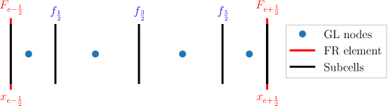
Figure 2: Subcells used by lower order scheme for degree $N=3$.

The MDRK scheme used in this work is fourth order accurate so we use polynomial degree $N=3$ in what follows, but write the procedure for general $N$. Let us subdivide each element $\Omega_{e}$ into $N+1$ subcells associated to the solution points $\{x^{e}_{p},p=0,1,\ldots,N\}$ of the MDRK scheme. Thus, we will have $N+2$ subfaces denoted by $\{x^{e}_{p+\frac{1}{2}},p=-1,0,\ldots,N\}$ with $x^{e}_{-\frac{1}{2}}=x_{e-\frac{1}{2}}$ and $x^{e}_{N+\frac{1}{2}}=x_{e+\frac{1}{2}}$. For maintaining a conservative scheme, the $p^{\operatorname{th}}$ subcell is chosen so that

$$x_{p+\frac{1}{2}}^{e}-x_{p-\frac{1}{2}}^{e}=w_{p}\Delta x_{e},\qquad 0\leq p\leq N$$ (24)

where $w_{p}$ is the $p^{\operatorname{th}}$ quadrature weight associated with the solution points. Figure 2 gives an illustration of the subcells for degree $N=3$ case. We explain the blending scheme for the second stage, where the lower order scheme performs evolution from $t^{n}$ to $t^{n+1}$. The low order scheme is obtained by updating the solution in each of the subcells by a finite volume scheme,

$$\begin{split}\bm{u}_{e,0}^{L,n+1}&=\bm{u}_{e,0}^{n}-\frac{\Delta t}{w_{0}\Delta x_{e}}[\bm{f}_{\frac{1}{2}}^{e}-\bm{F}_{e-\frac{1}{2}}]\\ \bm{u}_{e,p}^{L,n+1}&=\bm{u}_{e,p}^{n}-\frac{\Delta t}{w_{p}\Delta x_{e}}[\bm{f}_{p+\frac{1}{2}}^{e}-\bm{f}_{p-\frac{1}{2}}^{e}],\qquad 1\leq p\leq N-1\\ \bm{u}_{e,N}^{L,n+1}&=\bm{u}_{e,N}^{n}-\frac{\Delta t}{w_{N}\Delta x_{e}}[\bm{F}_{e+\frac{1}{2}}-\bm{f}_{N-\frac{1}{2}}^{e}]\end{split}$$ (25)

The inter-element fluxes $\bm{F}_{e+\frac{1}{2}}$ used in the low order scheme are same as those used in the high order MDRK scheme in equation (6). Usually, Rusanov’s flux [25] will be used for the inter-element fluxes and in the lower order scheme. The element mean value obtained by the low order scheme satisfies

$$\overline{\bm{u}}_{e}^{L,n+1}=\sum_{p=0}^{N}\bm{u}_{e,p}^{L,n+1}w_{p}=\overline{\bm{u}}_{e}^{n}-\frac{\Delta t}{\Delta x_{e}}(\bm{F}_{e+\frac{1}{2}}-\bm{F}_{e-\frac{1}{2}})$$ (26)

which is identical to the update equation by the MDRK scheme given in equation (8) in the absence of source terms. The element mean in the blended scheme evolves according to

$$\overline{\bm{u}}_{e}^{n+1} =(1-\alpha_{e})(\overline{\bm{u}}_{e})^{H,n+1}+\alpha_{e}(\overline{\bm{u}}_{e})^{L,n+1}$$

$$=(1-\alpha_{e})\left[\overline{\bm{u}}_{e}^{n}-\frac{\Delta t}{\Delta x_{e}}(\bm{F}_{e+\frac{1}{2}}-\bm{F}_{e-\frac{1}{2}})\right]+\alpha_{e}\left[\overline{\bm{u}}_{e}^{n}-\frac{\Delta t}{\Delta x_{e}}(\bm{F}_{e+\frac{1}{2}}-\bm{F}_{e-\frac{1}{2}})\right]$$

$$=\overline{\bm{u}}_{e}^{n}-\frac{\Delta t}{\Delta x_{e}}(\bm{F}_{e+\frac{1}{2}}-\bm{F}_{e-\frac{1}{2}})$$

and hence the blended scheme is also conservative. The similar arguments will apply to the first stage and we will have by (8)

$$\begin{split}\overline{\bm{u}}^{\ast}&=\overline{\bm{u}}_{e}^{n}-\frac{\Delta t}{\Delta x_{e}}(\bm{F}^{\ast}_{e+\frac{1}{2}}-\bm{F}^{\ast}_{e-\frac{1}{2}})\\ \overline{\bm{u}}_{e}^{n+1}&=\overline{\bm{u}}_{e}^{n}-\frac{\Delta t}{\Delta x_{e}}(\bm{F}_{e+\frac{1}{2}}-\bm{F}_{e-\frac{1}{2}})\end{split}$$ (27)

Overall, all three schemes, i.e., lower order, MDRK and the blended scheme, predict the same mean value.

The inter-element fluxes $\bm{F}^{\ast}_{e+\frac{1}{2}},\bm{F}_{e+\frac{1}{2}}$ are used both in the low and high order schemes. To achieve high order accuracy in smooth regions, this flux needs to be high order accurate, however it may produce spurious oscillations near discontinuities when used in the low order scheme. A natural choice to balance accuracy and oscillations is to take

$$\begin{split}\bm{F}_{e+\frac{1}{2}}&=(1-\alpha_{e+\frac{1}{2}})\bm{F}^{\operatorname{HO}\ast}_{e+\frac{1}{2}}+\alpha_{e+\frac{1}{2}}\bm{f}_{e+\frac{1}{2}}\\ \bm{F}_{e+\frac{1}{2}}&=(1-\alpha_{e+\frac{1}{2}})\bm{F}_{e+\frac{1}{2}}^{\operatorname{HO}}+\alpha_{e+\frac{1}{2}}\bm{f}_{e+\frac{1}{2}}\end{split}$$ (28)

where $\bm{F}^{\operatorname{HO}\ast}_{e+\frac{1}{2}},\bm{F}_{e+\frac{1}{2}}^{\operatorname{HO}}$ are the high order inter-element time-averaged numerical fluxes used in the MDRK scheme (13) and $\bm{f}_{e+\frac{1}{2}}$ is a lower order flux at the face $x_{e+\frac{1}{2}}$ shared between FR elements and subcells (29, 30). The blending coefficient $\alpha_{e+\frac{1}{2}}$ will be based on a local smoothness indicator which will bias the flux towards the lower order flux $\bm{f}_{e+\frac{1}{2}}$ near regions of lower solution smoothness. However, to enforce admissibility in means (Definition 2), the flux has to be further corrected, as explained in Section 6.3.

6.1 First order blending

The lower order scheme is taken to be a first order finite volume scheme, for which the subcell fluxes in (25) are given by

$$\bm{f}_{e+\frac{1}{2}}^{e}=\bm{f}(\bm{u}_{e,p},\bm{u}_{e,p+1})$$

At the interfaces that are shared with FR elements, we define the lower order flux used in computing inter-element flux as

$$\bm{f}_{e+\frac{1}{2}}=\bm{f}(\bm{u}_{e,N},\bm{u}_{e+1,0})$$ (29)

In this work, the numerical flux $\bm{f}(\cdot,\cdot)$ is taken to be Rusanov’s flux [25], which is the same flux used by the higher order scheme at the element interfaces.

6.2 Higher order blending

The MUSCL-Hancock scheme uses a flux whose stencil is given by

$$\bm{f}_{e+\frac{1}{2}}=\bm{f}(\bm{u}_{e,N-1},\bm{u}_{e,N},\bm{u}_{e+1,0},\bm{u}_{e+1,1})$$ (30)

Since the evolution in first stage is from $t^{n}$ to $t^{n+\frac{1}{2}}$ and in the second from $t^{n}$ to $t^{n+1}$, the procedure remains the smae for both stages. Thus, the details of the construction of an admissibility preserving MUSCL-Hancock flux on the non-uniform non-cell centred subcells involved in the blending scheme can be found in [4].

6.3 Flux limiter

The flux limiter to enforce admissibility will be applied in each stage so that the evolution of each stage is admissibility preserving. Thus, the admissibility enforcing flux limiting procedure of [4] applied to each stage of MDRK ensures admissibility of that stage and thus of the overall scheme. Since the blending is performed at each stage, the procedure remains the same as in the single stage method of [4] and the reader is referred to the same for details.

7 Numerical results

In this section, we test the MDRK scheme with numerical experiments using polynomial degree $N=3$ in all results. Most of the test cases from [3, 4] were tried and were seen to validate our claims; but we only show the important results here. We also tested all the benchmark problems for higher order methods in [20], and show some of the results from there.

7.1 Scalar equations

We perform convergence tests with scalar equations. The MDRK scheme with D1 and D2 dissipation are tested using the optimal CFL numbers from Table 1. We make comparison with RKFR scheme with polynomial degree $N=3$ described in Section 3 using the SSPRK scheme from [30]. The CFL number for the fourth order RK scheme is taken from [12]. In many problems, we compare with Gauss-Legendre (GL) solution points and Radau correction functions, and Gauss-Legendre-Lobatto (GLL) solution points with $g_{2}$ correction functions. These combinations are important because they are both variants of Discontinuous Galerkin methods [16, 10].

7.1.1 Linear advection equation

The initial condition $u(x,0)=\sin(2\pi x)$ is taken with periodic boundaries on $[0,1]$. The error norms are computed at time $t=2$ units and shown in Figure 3. The MDRK scheme with D2 dissipation (MDRK-D2) scheme shows optimal order of convergence and has errors close to that MDRK-D1 and the RK scheme for all the combinations of solution points and correction functions.

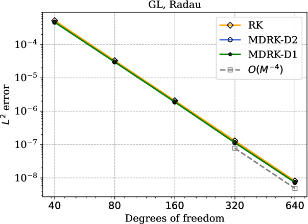
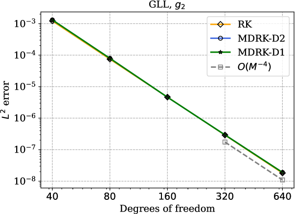
(a)	(b)

Figure 3: Error convergence for constant linear advection equation comparing MDRK and RK - (a) GL points with Radau correction, (b) GLL points with $g_{2}$ correction

7.1.2 Variable advection equation

$$u_{t}+f(x,u)_{x}=0,\qquad f(x,u)=a(x)u$$

The velocity is $a(x)=x^{2}$, $u_{0}(x)=\cos(\pi x/2)$, $x\in[0.1,1]$ and the exact solution is $u(x,t)=u_{0}(x/(1+tx))/(1+tx)^{2}$. Dirichlet boundary conditions are imposed on the left boundary and outflow boundary conditions on the right. This problem is non-linear in the spatial variable, i.e., if $I_{h}$ is the interpolation operator, $I_{h}(au_{h})\neq I_{h}(a)I_{h}(u_{h})$. Thus, the AE and EA schemes are expected to show different behavior, unlike the previous test.

The grid convergence analysis is shown in Figure 4. In Figure 4a, the scheme with AE shows larger errors compared to the RK scheme though the convergence rate is optimal. The MDRK scheme with EA shown in the middle figure, is as accurate as the RK scheme. The last figure compares AE and EA schemes using GL solution points, Radau correction function and D2 dissipation; we clearly see that EA scheme has smaller errors than AE scheme.

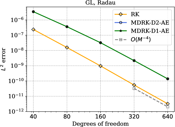
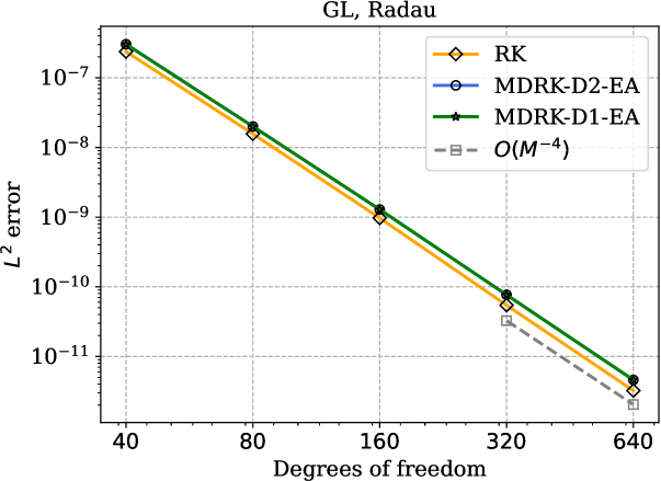
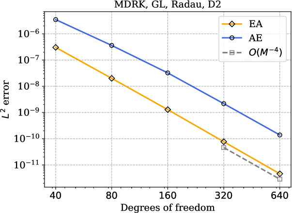
(a)	(b)	(c)

Figure 4: Error convergence for variable linear advection equation with $a(x)=x^{2}$; (a) AE scheme, (b) EA scheme, (c) AE versus EA

7.1.3 Burgers’ equations

The one dimensional Burger’s equation is a conservation law of the form $u_{t}+f(u)_{x}=0$ with the quadratic flux $f(u)=u^{2}/2$. For the smooth initial condition $u(x,0)=0.2\sin(x)$ with periodic boundary condition in the domain $[0,2\pi]$, we compute the numerical solution at time $t=2.0$ when the solution is still smooth. Figure 5a compares the error norms for the AE and EA methods for the Rusanov numerical flux, and using GL solution points, Radau correction and D2 dissipation. The convergence rate of AE is less than optimal and close to $O(h^{3+1/2})$. In Figure 5b, we see that no scheme shows optimal convergence rates when $g_{2}$ correction + GLL points is used. The comparison between D1, D2 dissipation is made in Figure 6 and their performances are found to be similar.

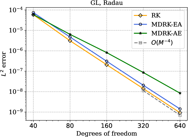
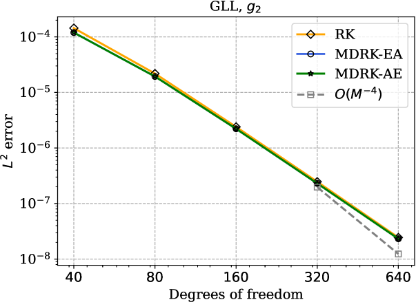
(a)	(b)

Figure 5: Comparing AE and EA schemes using D2 dissipation for 1-D Burgers’ equation at $t=2$. (a) GL points with Radau correction, (b) GLL points with $g_{2}$ correction

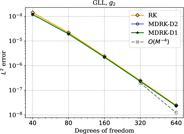
(a)	(b)

Figure 6: Comparing D1 and D2 dissipation for 1-D Burgers’ equation at $t=2$. (a) GL points with Radau correction, (b) GLL points with $g_{2}$ correction

7.2 1-D Euler equations

As an example of system of non-linear hyperbolic equations, we consider the one-dimensional Euler equations of gas dynamics given by

$$\frac{\partial}{\partial t}\left(\begin{array}[]{c}\rho\\ \rho u\\ E\end{array}\right)+\frac{\partial}{\partial x}\left(\begin{array}[]{c}\rho u\\ p+\rho u^{2}\\ (E+p)u\end{array}\right)=\bm{0}$$ (31)

where $\rho,u,p$ and $E$ denote the density, velocity, pressure and total energy of the gas, respectively. For a polytropic gas, an equation of state $E=E(\rho,u,p)$ which leads to a closed system is given by

$$E=E(\rho,u,p)=\frac{p}{\gamma-1}+\frac{1}{2}\rho u^{2}$$ (32)

where $\gamma>1$ is the adiabatic constant, that will be taken as $1.4$ which is the value for air. In the following results, wherever it is not mentioned, we use the Rusanov flux. We use Radau correction function with Gauss-Legendre solution points in this section because of their superiority seen in [3, 4]. The time step size is taken to be

$$\Delta t=C_{s}\min_{e}\left(\frac{\Delta x_{e}}{|\bar{v}_{e}|+\bar{c}_{e}}\right)\text{CFL}$$ (33)

where $e$ is the element index, $\bar{v}_{e},\bar{c}_{e}$ are velocity and sound speed of element mean in element $e$, CFL=0.107 (Table 1). The coefficient $C_{s}=0.98$ is used in tests, unless specified otherwise.

7.2.1 Blast

The Euler equations (31) are solved with the initial condition

$$(\rho,v,p)=\begin{cases}(1,0,1000),&\text{if }x<0.1\\ (1,0,0.01),&\text{if }0.1<x<0.9\\ (1,0,100),&\text{if }x>0.9\end{cases}$$

in the domain $[0,1]$. This test was originally introduced in [38] to check the capability of the numerical scheme to accurately capture the shock-shock interaction scenario. The boundaries are set as solid walls by imposing the reflecting boundary conditions at $x=0$ and $x=1$. The solution consists of reflection of shocks and expansion waves off the boundary wall and several wave interactions inside the domain. The numerical solutions give negative pressure if the positivity correction is not applied. With a grid of 400 cells using polynomial degree $N=3$, we run the simulation till the time $t=0.038$ where a high density peak profile is produced. As tested in [4], we compare first order (FO) and MUSCL-Hancock (MH) blending schemes, and TVB limiter with parameter $M=300$ [21] (TVB-300). We compare the performance of limiters in Figure (7) where the approximated density and pressure profiles are compared with a reference solution computed using a very fine mesh. Looking at the peak amplitude and contact discontinuity, it is clear that MUSCL-Hancock blending scheme gives the best resolution, especially when compared with the TVB limiter.

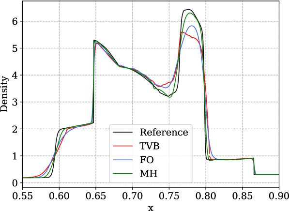
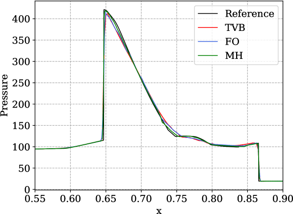
(a)	(b)

Figure 7: Blast wave problem using first order (FO) and MUSCL-Hancock blending schemes, and TVB limited scheme (TVB-300) with parameter $M=300$. (a) Density, (b) Pressure profiles are shown at $t=0.038$ on a mesh of 400 cells.

7.2.2 Titarev Toro

This is an extension of the Shu-Osher problem given by Titarev and Toro [33] and the initial data comprises of a severely oscillatory wave interacting with a shock. This problem tests the ability of a high-order numerical scheme to capture the extremely high frequency waves. The smooth density profile passes through the shock and appears on the other side, and its accurate computation is challenging due to numerical dissipation. Due to presence of both spurious oscillations and smooth extrema, this becomes a good test for testing robustness and accuracy of limiters. We discretize the spatial domain with 800 cells using polynomial degree $N=3$ and compare blending schemes. As expected, the MUSCL-Hancock (MH) blending scheme is superior to the First Order (FO) blending scheme and has nearly resolved in the smooth extrema.

The initial condition is given by

$$(\rho,v,p)=\begin{cases}(1.515695,0.523346,1.805),\qquad&-5\leq x\leq-4.5\\ (1+0.1\sin(20\pi x),0,1),&-4.5<x\leq 5\end{cases}$$

The physical domain is $[-5,5]$ and a grid of 800 elements is used. The density profile at $t=5$ is shown in Figure 8.

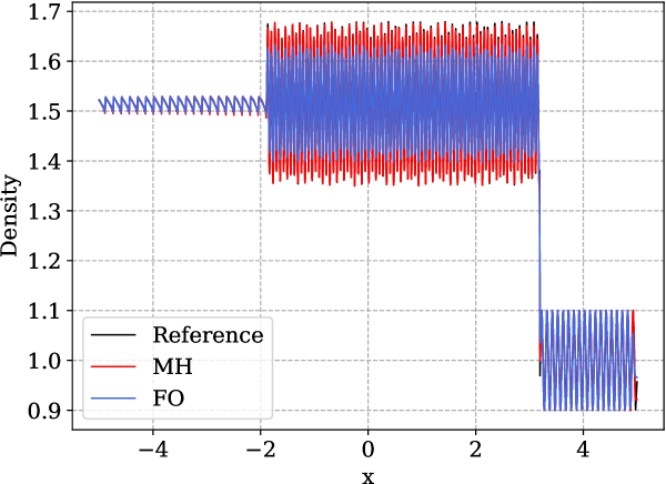
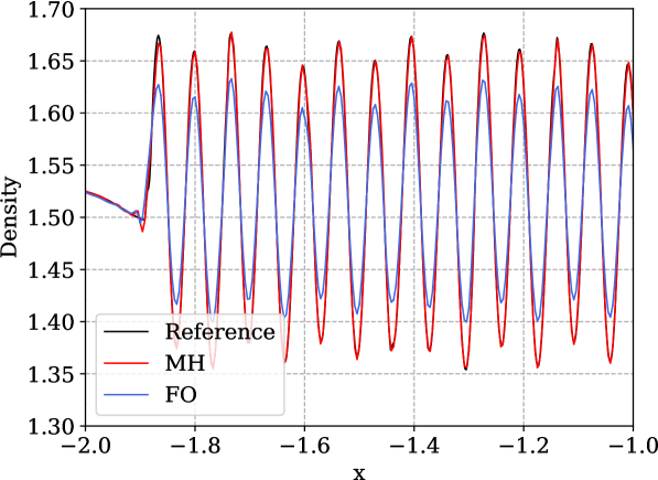
(a)	(b)

Figure 8: Titarev-Toro problem, comparing First Order (FO) and MUSCL-Hancock (MH) blending (a) Complete plot, (b) Profile zoomed near smooth extrema on a mesh of 800 cells.

7.2.3 Large density ratio Riemann problem

The second example is the large density ratio problem with a very strong rarefaction wave [32]. The initial condition is given by

$$(\rho,v,p)=\begin{cases}(1000,0,1000),\quad&x<0.3\\ (1,0,1),&0.3<x\end{cases}$$

The computational domain is $[0,1]$ and transmissive boundary condition is used at both ends. The density and pressure profile on a mesh of $500$ elements at $t=0.15$ is shown in Figure 9. The MH blending scheme is giving better accuracy even in this tough problem.

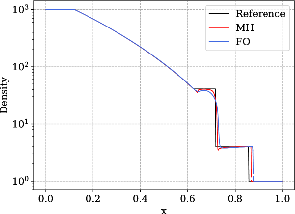
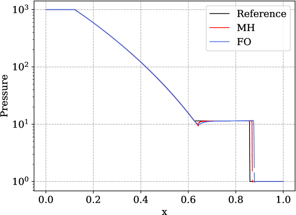
(a)	(b)

Figure 9: High density problem at $t=0.15$ on a mesh of 500 elements (a) Density plot, (b) Pressure plot

7.2.4 Sedov’s blast

To demonstrate the admissibility preserving property of our scheme, we simulate Sedov’s blast wave [27]; the test describes the explosion of a point-like source of energy in a gas. The explosion generates a spherical shock wave that propagates outwards, compressing the gas and reaching extreme temperatures and pressures. The problem can be formulated in one dimension as a special case, where the explosion occurs at $x=0$ and the gas is confined to the interval $[-1,1]$ by solid walls. For the simulation, on a grid of 201 cells with solid wall boundary conditions, we use the following initial data [41],

$$\rho=1,\qquad v=0,\qquad E(x)=\left\{\begin{array}[]{ll}\frac{3.2\times 10^{6}}{\Delta x},&|x|\leq\frac{\Delta x}{2}\\ 10^{-12},&\text{otherwise}\end{array}\right.$$

where $\Delta x$ is the element width. This is a difficult test for positivity preservation because of the high pressure ratios. Nonphysical solutions are obtained if the proposed admissibility preservation corrections are not applied. The density and pressure profiles at $t=0.001$ are obtained using blending schemes are shown in Figure 10. In [4], TVB limiter could not be used in this test as the proof of admissibility preservation depended on the blending scheme. Here, by using the generalized admissibility preserving scheme of [2] to be able to use the TVB limiter. However, we TVB limiter being less accurate and unable to control the oscillations..

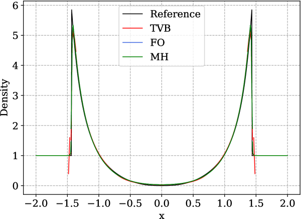
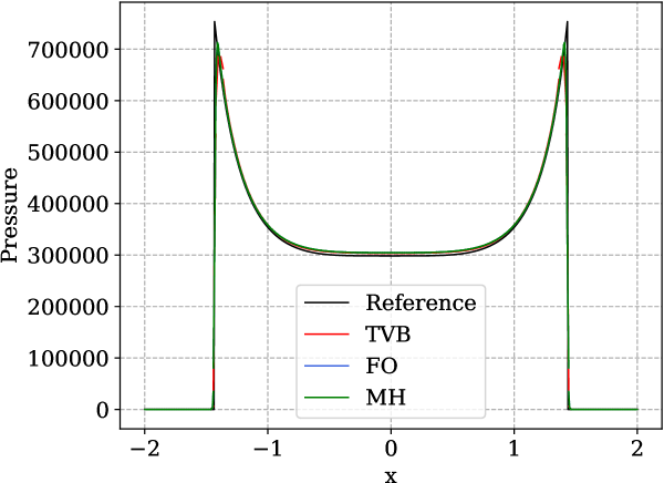
(a)	(b)

Figure 10: Sedov’s blast wave problem, numerical solution using first order (FO) and MUSCL-Hancock blending schemes, and TVD (a) Density, (b) Pressure profiles are shown at $t=0.001$ on a mesh of 201 cells

7.3 2-D Euler’s equations

We consider the two-dimensional Euler equations of gas dynamics given by

$$\frac{\partial}{\partial t}\left(\begin{array}[]{c}\rho\\ \rho u\\ \rho v\\ E\end{array}\right)+\frac{\partial}{\partial x}\left(\begin{array}[]{c}\rho u\\ p+\rho u^{2}\\ \rho uv\\ (E+p)u\end{array}\right)+\frac{\partial}{\partial y}\left(\begin{array}[]{c}\rho v\\ \rho uv\\ p+\rho v^{2}\\ (E+p)v\end{array}\right)=\bm{0}$$ (34)

where $\rho,p$ and $E$ denote the density, pressure and total energy of the gas, respectively and $(u,v)$ are Cartesian components of the fluid velocity. For a polytropic gas, an equation of state $E=E(\rho,u,v,p)$ which leads to a closed system is given by

$$E=E(\rho,u,v,p)=\frac{p}{\gamma-1}+\frac{1}{2}\rho(u^{2}+v^{2})$$ (35)

where $\gamma>1$ is the adiabatic constant, that will be taken as $1.4$ in the numerical tests, which is the typical value for air. The time step size for polynomial degree $N$ is computed as

$$\Delta t=C_{s}\min_{e}\left(\frac{|\bar{u}_{e}|+\bar{c}_{e}}{\Delta x_{e}}+\frac{|\bar{v}_{e}|+\bar{c}_{e}}{\Delta y_{e}}\right)^{-1}\text{CFL}$$ (36)

where $e$ is the element index, $(\bar{u}_{e},\bar{v}_{e}),\bar{c}_{e}$ are velocity and sound speed of element mean in element $e$, CFL=0.107 (Table 1) and $C_{s}\leq 1$ is a safety factor.

For verification of some our numerical results and to demonstrate the accuracy gain observed in [4] of using MUSCL-Hancock reconstruction using Gauss-Legendre points, we will compare our results with the first order blending scheme using Gauss-Legendre-Lobatto (GLL) points of [15] available in Trixi.jl [23]. The accuracy benefit is expected since GL points and quadrature are more accurate than GLL points, and MUSCL-Hancock is also more accurate than first order finite volume method.

7.3.1 Double Mach reflection

This test case was originally proposed by Woodward and Colella [38] and consists of a shock impinging on a wedge/ramp which is inclined by 30 degrees. An equivalent problem is obtained on the rectangular domain $\Omega=[0,4]\times[0,1]$ obtained by rotating the wedge so that the initial condition now consists of a shock angled at 60 degrees. The solution consists of a self similar shock structure with two triple points. Define $\bm{u}_{b}=\bm{u}_{b}(x,y,t)$ in primitive variables as

$$(\rho,u,v,p)=\begin{cases}(8,8.25\cos(\frac{\pi}{6}),-8.25\sin(\frac{\pi}{6}),116.5),&\text{if }x<\frac{1}{6}+\frac{y+20t}{\sqrt{3}}\\ (1.4,0,0,1),&\text{if }x>\frac{1}{6}+\frac{y+20t}{\sqrt{3}}\end{cases}$$

and take the initial condition to be $\bm{u}_{0}(x,y)=\bm{u}_{b}(x,y,0)$. With $\bm{u}_{b}$, we impose inflow boundary conditions at the left side $\{0\}\times[0,1]$, outflow boundary conditions both on $[0,1/6]\times\{0\}$ and $\{4\}\times[0,1]$, reflecting boundary conditions on $[1/6,4]\times\{0\}$ and inflow boundary conditions on the upper side $[0,4]\times\{1\}$.

The simulation is run on a mesh of $600\times 150$ elements using degree $N=3$ polynomials up to time $t=0.2$. In Figure 11, we compare the results of Trixi.jl with the MUSCL-Hancock blended scheme zoomed near the primary triple point. As expected, the small scale structures are captured better by the MUSCL-Hancock blended scheme.

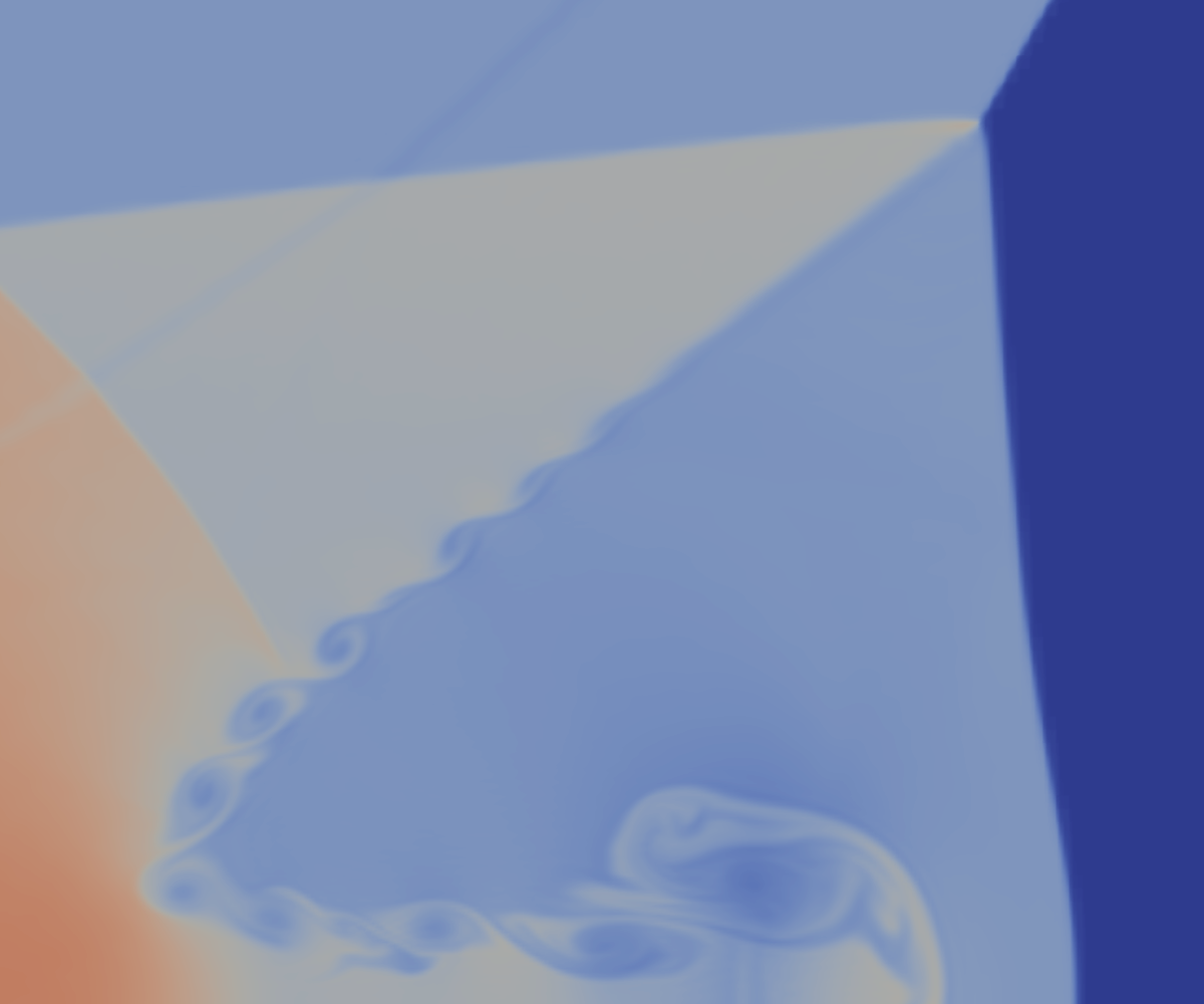
(a) MDRK	(b) Trixi.jl

Figure 11: Double Mach reflection problem, density plot of numerical solution at $t=0.2$ on a $600\times 150$ mesh zoomed near the primary triple point.

7.3.2 Rotational low density problem

This problems are taken from [20] where the solution consists of hurricane-like flow evolution, where solution has one-point vacuum in the center with rotational velocity field. The initial condition is given by

$$(\rho,u,v,p)=(\rho_{0},v_{0}\sin\theta,-v_{0}\cos\theta,A\rho_{0}^{\gamma})$$

where $\theta=\arctan(y/x)$, $A=25$ is the initial entropy, $\rho=1$ is the initial density, gas constant $\gamma=2$. The initial velocity distribution has a nontrivial transversal component, which makes the flow rotational. The solutions are classified [40] into three types according to the initial Mach number $M_{0}=|v_{0}|/c_{0}$, where $c_{0}=p^{\prime}(\rho_{0})=A\gamma\rho_{0}^{\gamma-1}$ is the sound speed.

1. Critical rotation with $M_{0}=\sqrt{2}$. This test has an exact solution with explicit formula. The solution consists of two parts: a far field solution and a near-field solution. The former far field solution is defined for $r\geq 2t\sqrt{p^{\prime}(\rho_{0})}$, $r=\sqrt{x^{2}+y^{2}}$,

   $$\begin{split}U(x,y,t)&=\frac{1}{r}(2tp_{0}^{\prime}\cos\theta+\sqrt{2p_{0}^{\prime}}\sqrt{r^{2}-2t^{2}p_{0}^{\prime}}\sin\theta)\\ V(x,y,t)&=\frac{1}{r}(2tp_{0}^{\prime}\sin\theta-\sqrt{2p_{0}^{\prime}}\sqrt{r^{2}-2t^{2}p_{0}^{\prime}}\cos\theta)\\ \rho(x,y,t)&=\rho_{0}\\ p(x,y,t)&=A\rho_{0}^{\gamma}\end{split}$$ (37)

   and the near-field solution is defined for $r<2t\sqrt{p^{\prime}(\rho_{0})}$

   $$U(x,y,t)=\frac{x+y}{2t},\quad V(x,y,t)=\frac{-x+y}{2t},\quad\rho(x,y,t)=\frac{r^{2}}{8At^{2}}$$

   The curl of the velocity in the near-field is

   $$\operatorname{curl}(U,V)=V_{x}-U_{y}=-\frac{1}{2t}\neq 0$$

   and the solution has one-point vacuum at the origin $r=0$. This is typical hurricane-like solution that behaves highly singular, particularly near the origin $r=0$. There are two issues here challenging the numerical schemes: one is the presence of the vacuum state which examines whether a high order scheme can keep the positivity preserving property; the other is the rotational velocity field for testing whether a numerical scheme can preserve the symmetry. In this regime, we take $v_{0}=10$ on the computational domain $[-1,1]^{2}$ with $\Delta x=\Delta y=1/100$. The boundary condition is given by the far field solution in (37).

2. High-speed rotation with $M_{0}>\sqrt{2}$. For this case, $v_{0}=12.5$, so that the density goes faster to the vacuum and the fluid rotates severely. The physical domain is $[-2,2]^{2}$ and the grid spacing is $\Delta x=\Delta y=1/100$. Outflow boundary conditions are given on the boundaries.Because of the higher rotation speed, this case is tougher than the first one, and can be used to validate the robustness of the higher-order scheme.

3. Low-speed rotation with $M_{0}<\sqrt{2}$. In this test case, we take $v_{0}=7.5$ making it a rotation with lower speed than the previous tests. The outflow boundary conditions are given as in the previous tests. The simulation is performed in the domain $[-1,1]^{2}$ till $t=0.045$. The symmetry of flow structures is preserved.

The density profile for the flow with critical speed are shown in Figure 12 including a comparison with exact solution at a line cut of $y=0$ in Figure 12b, showing near overlap. In Figure 13a, we show the line cut of density profile at $y=0$ for the three rotation speeds. In Figure 13b, we show streamlines for high rotational speed, showing symmetry.

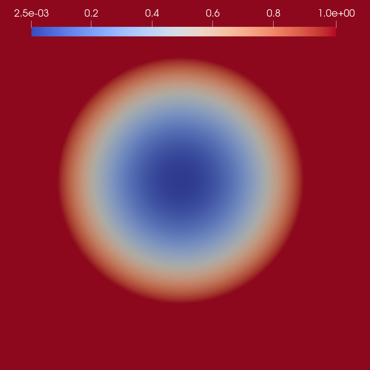
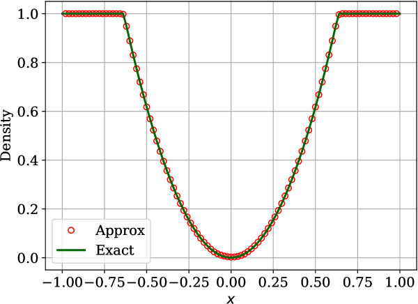
(a)	(b)

Figure 12: Density profile of rotational low density problem at critical speed (a) Pseudocolor plot (b) Line cut at $y=0$ on a mesh with $\Delta x=\Delta y=1/100$.

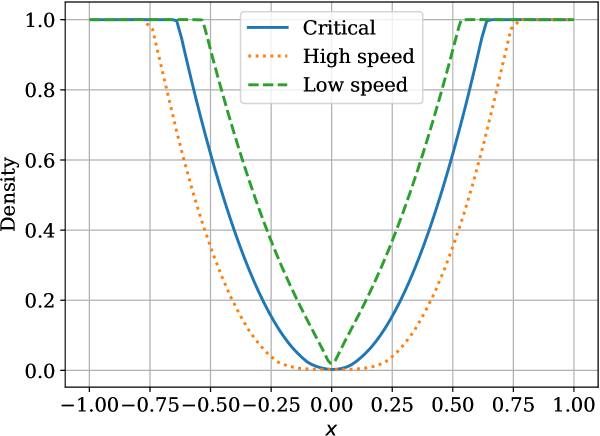
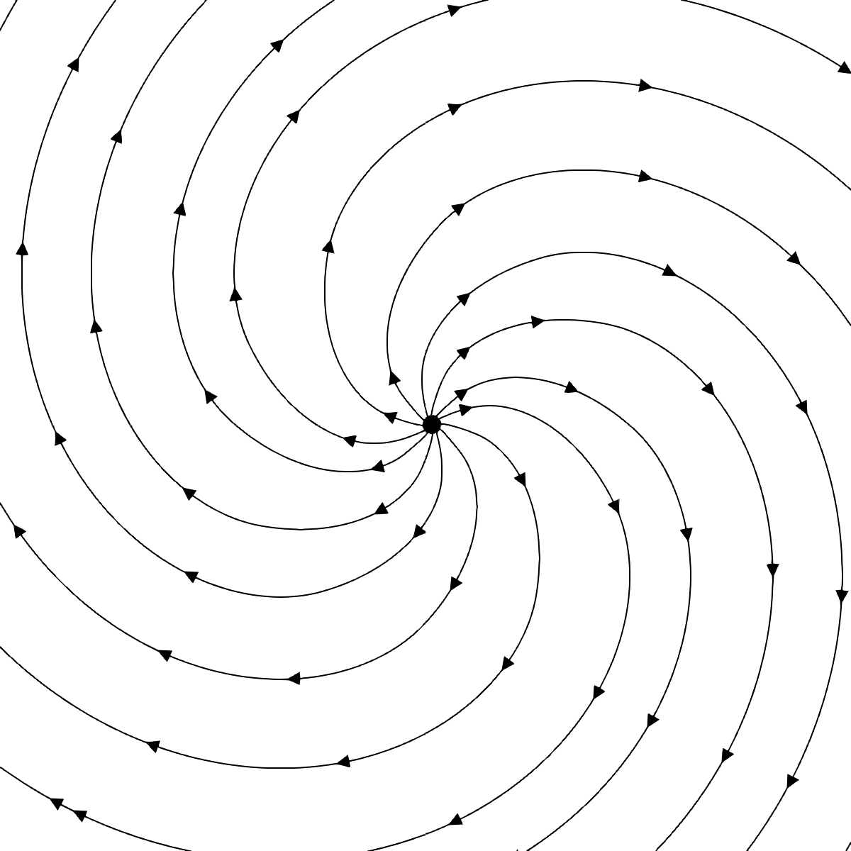
(a)	(b)

Figure 13: Rotational low density problem (a) Density profile line cut at $y=0$ for different rotational speeds, (b) Stream lines for high rotational speed

7.3.3 Two Dimensional Riemann problem

2-D Riemann problems consist of four constant states and have been studied theoretically and numerically for gas dynamics in [13]. We consider this problem in the square domain $[0,1]^{2}$ where each of the four quadrants has one constant initial state and every jump in initial condition leads to an elementary planar wave, i.e., a shock, rarefaction or contact discontinuity. There are only 19 such genuinely different configurations possible [39, 17]. As studied in [39], a bounded region of subsonic flows is formed by interaction of different planar waves leading to appearance of many complex structures depending on the elementary planar flow. We consider configuration 12 of [17] consisting of 2 positive slip lines and two forward shocks, with initial condition

$$(\rho,u,v,p)=\begin{cases}(0.5313,0,0,0.4)\qquad&\text{if }x\geq 0.5,y\geq 0.5\\ (1,0.7276,0,1)&\text{if }x<0.5,y\geq 0.5\\ (0.8,0,0,1)&\text{if }x<0.5,y<0.5\\ (1,0,0.7276,1)&\text{if }x\geq 0.5,y<0.5\end{cases}$$

The simulations are performed with transmissive boundary conditions on an enlarged domain upto time $t=0.25$. The density profiles obtained from the MUSCL-Hancock blending scheme and Trixi.jl are shown in Figure 14. We see that both schemes give similar resolution in most regions. The MUSCL-Hancock blending scheme gives better resolution of the small scale structures arising across the slip lines.

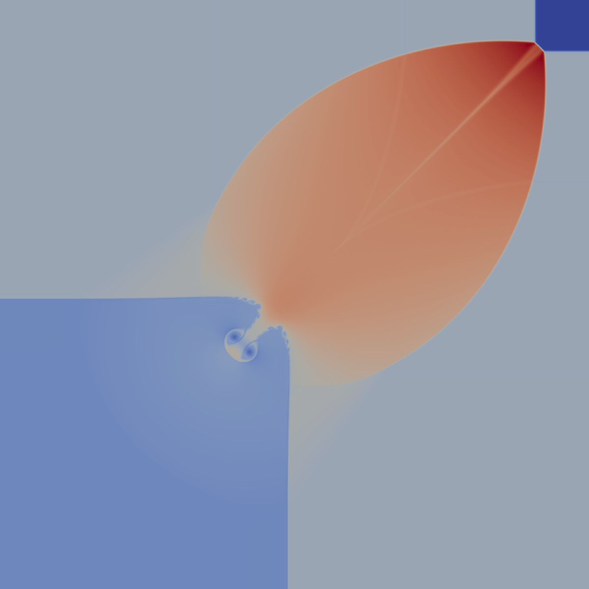
(a)	(b)
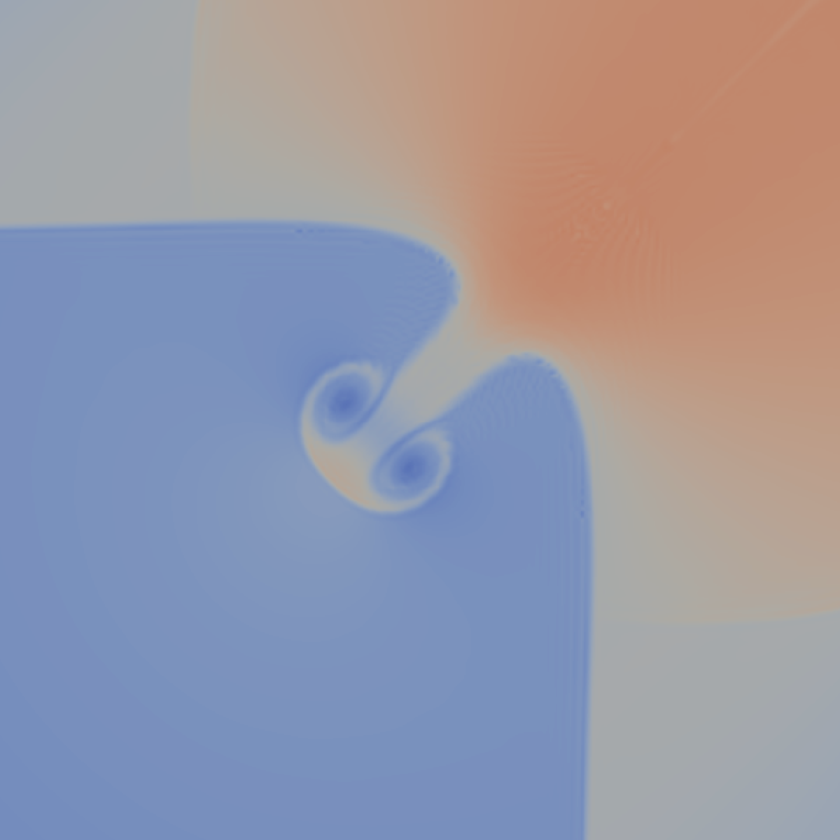
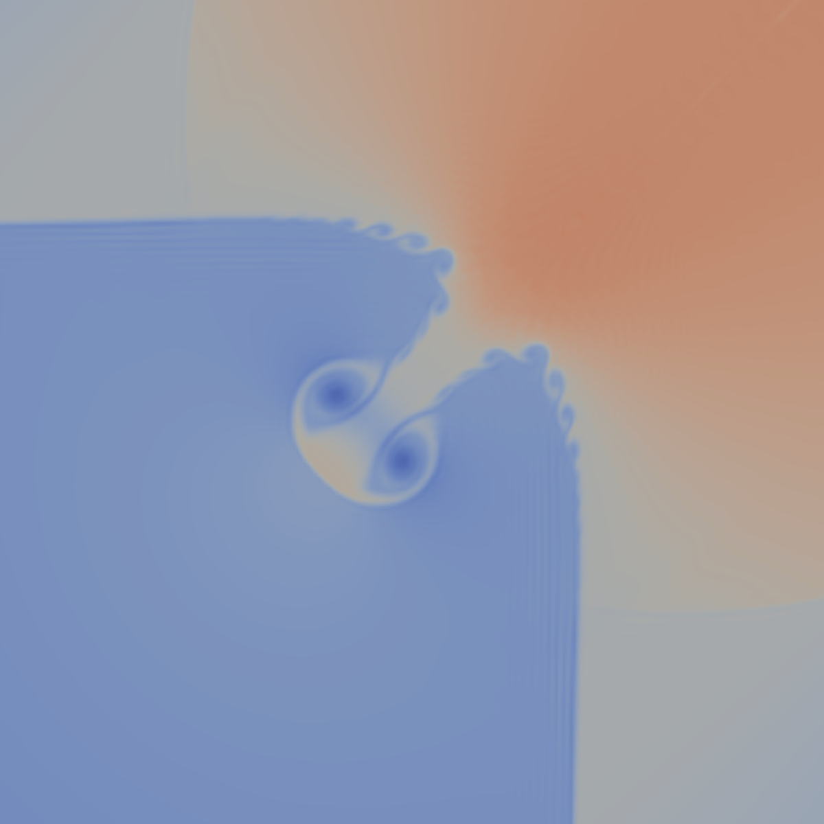
(c)	(d)

Figure 14: 2-D Riemann problem, density plots of numerical solution at $t=0.25$ for degree $N=3$ on a $256\times 256$ mesh (a) Trixi.jl, (b) MDRK, (c) Trixi.jl zoomed, (d) MDRK zoomed

7.3.4 Rayleigh-Taylor instability

The last problem is the Rayleigh-Taylor instability to test the performance of higher-order scheme for the conservation laws with source terms, and the governing equations are written as

$$\frac{\partial}{\partial t}\left(\begin{array}[]{c}\rho\\ \rho u\\ \rho v\\ E\end{array}\right)+\frac{\partial}{\partial x}\left(\begin{array}[]{c}\rho u\\ p+\rho u^{2}\\ \rho uv\\ (E+p)u\end{array}\right)+\frac{\partial}{\partial y}\left(\begin{array}[]{c}\rho v\\ \rho uv\\ p+\rho v^{2}\\ (E+p)v\end{array}\right)=\left(\begin{array}[]{c}0\\ 0\\ \rho\\ \rho v\end{array}\right)$$

The implementation of MDRK with source terms is based on [2] where an approximate Lax-Wendroff procedure is also applied on the source term. The following description is taken from [20]. The Rayleigh-Taylor instability happens on the interface between fluids with different densities when an acceleration is directed from the heavy fluid to the light one. The instability with fingering nature generates bubbles of light fluid rising into the ambient heavy fluid and spikes of heavy fluid falling into the light fluid. The initial condition of this problem [28] is given as follows

$$(\rho,u,v,p)=\begin{cases}(2,0,-0.025a\cos(8\pi x),2y+1),\quad&y\leq 0.5,\\ (1,0,-0.025a\cos(8\pi x),y+1.5),&y>0.5\end{cases}$$

where $a=\sqrt{\gamma p/\rho}$ is the sound speed and $\gamma=5/3$. The computational domain is $[0,0.25]\times[0,1]$. The reflecting boundary conditions are imposed for the left and right boundaries. At the top boundary, the flow variables are set as $(\rho,u,v,p)=(1,0,0,2.5)$. At the bottom boundary, they are $(\rho,u,v,p)=(2,0,0,1)$. The uniform mesh with $64\times 256$ elements is used in the simulation. The density distributions at $t=1.5,1.75,2,2.25,2.5$ are presented in Figure 15. It is a test to check the suitability of higher-order schemes for the capturing of interface instabilities.

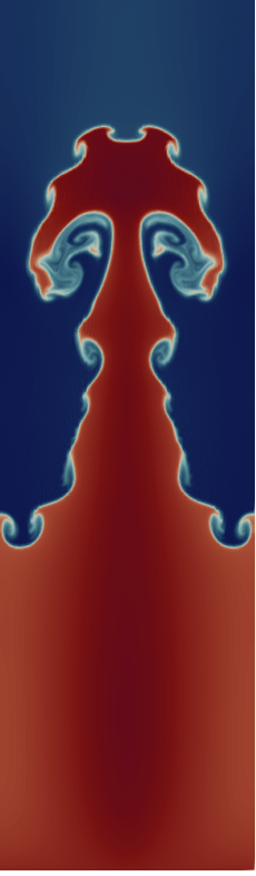
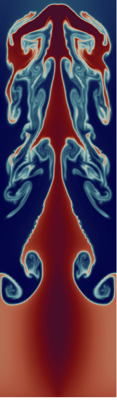
(a) $t=1.5$	(b) $t=1.75$	(c) $t=2$	(d) $t=2.25$	(e) $t=2.5$

Figure 15: Rayleigh-Taylor instability on a $64\times 256$ mesh

8 Summary and conclusions

This work introduces fourth order multiderivative Runge-Kutta (MDRK) scheme of [18] in the conservative, quadrature free Flux Reconstruction framework to solve hyperbolic conservation laws. The idea is to cast each MDRK stage as an evolution involving a time average flux which is approximated by the Jacobian free Approximate Lax-Wendroff procedure. The numerical flux is carefully computed with accuracy and stability in mind. In particular, the D2 dissipation and EA flux of [3] have been introduced which enhance stable CFL numbers and accuracy for nonlinear problems respectively. The stable CFL numbers are computed using Fourier stability analysis for two commonly used correction functions $g_{\operatorname{Radau}}$ and $g_{2}$, showing the improved CFL numbers. Convergence analysis for non-linear problems was performed which revealed that optimal convergence rates were only shown when using the EA flux. The shock capturing blending scheme of [4] has also been introduced for the MDRK scheme applied at each stage. The scheme is provably admissibility preserving and good at capturing small scale structures. The claims are validated by numerical experiments.

Appendix A Formal accuracy analysis

We consider the system of time dependent equations

$$\bm{u}_{t}=\bm{L}\left(\bm{u}\right)$$

which relates to the hyperbolic conservation law (1) by setting $\bm{L}=-\bm{f}\left(\bm{u}\right)_{x}$. Now, we are analyzing the scheme

$$\begin{split}\bm{u}^{\ast}&=\bm{u}^{n}+\Delta ta_{21}\bm{L}\left(\bm{u}^{n}\right)+\Delta t^{2}\hat{a}_{21}\bm{L}_{t}\left(\bm{u}^{n}\right)\\ \bm{u}^{n+1}&=\bm{u}^{n}+\Delta t\left(b_{1}\bm{L}\left(\bm{u}^{n}\right)+b_{2}\bm{L}\left(\bm{u}^{\ast}\right)\right)+\Delta t^{2}\left(\hat{b}_{1}\partial_{t}\bm{L}+\hat{b}_{2}\partial_{t}\bm{L}\left(\bm{u}^{\ast}\right)\right)\end{split}$$ (38)

Further note that, we use the Approximate Lax-Wendroff (Section 4.3) to approximate $\partial_{t}\bm{L}\left(\bm{u}^{n}\right),\partial_{t}\bm{L}\left(\bm{u}^{\ast}\right)$ to $O(\Delta t^{3})$ accuracy and thus we perform an error analysis of an evolution performed as

$$\bm{u}^{\ast}=\bm{u}^{n}+\Delta ta_{21}\bm{L}\left(\bm{u}^{n}\right)+\Delta t^{2}\hat{a}_{21}\bm{L}_{t}\left(\bm{u}^{n}\right)+O(\Delta t^{5})$$

$$\bm{u}^{n+1}=\bm{u}^{n}+\Delta t\left(b_{1}\bm{L}\left(\bm{u}^{n}\right)+b_{2}\bm{L}\left(\bm{u}^{\ast}\right)\right)+\Delta t^{2}\left(\hat{b}_{1}\partial_{t}\bm{L}+\hat{b}_{2}\partial_{t}\bm{L}\left(\bm{u}^{\ast}\right)\right)+O(\Delta t^{5})$$ (39)

Now, note that

$$\begin{split}\bm{u}_{tt}=\bm{L}_{\bm{u}}\bm{u}_{t}=\bm{L}_{\bm{u}}\bm{L},\qquad\bm{u}_{ttt}=\bm{L}_{\bm{u}\bm{u}}\bm{u}_{t}^{2}+\bm{L}_{\bm{u}}\bm{u}_{tt}=\bm{L}_{\bm{u}\bm{u}}\bm{L}^{2}+\bm{L}_{\bm{u}}^{2}\bm{L}\\ \bm{u}_{tttt}=\bm{L}_{\bm{u}\bm{u}\bm{u}}\bm{u}_{t}^{3}+3\bm{L}_{\bm{u}\bm{u}}\bm{u}_{t}\bm{u}_{tt}+\bm{L}_{\bm{u}}\bm{u}_{ttt}=\bm{L}_{\bm{u}\bm{u}\bm{u}}\bm{L}^{3}+4\bm{L}_{\bm{u}\bm{u}}\bm{L}_{\bm{u}}\bm{L}^{2}+\bm{L}_{\bm{u}}^{3}\bm{L}\end{split}$$ (40)

Starting from $\bm{u}=\bm{u}^{n}$, the exact solution satisfies

$$\bm{u}^{n+1}=\bm{u}+\Delta t\bm{u}_{t}+\frac{\Delta t^{2}}{2}\bm{u}_{tt}+\frac{\Delta t^{3}}{6}\bm{u}_{ttt}+\frac{\Delta t^{4}}{24}\bm{u}_{tttt}+O(\Delta t^{5})$$ (41)

We note the following identities

$$\partial_{t}\bm{L}\left(\bm{u}\right)=\bm{L}_{\bm{u}}\bm{u}_{t}$$

$$\bm{u}^{\ast}=\bm{u}+\Delta ta_{21}\bm{L}+\Delta t^{2}\hat{a}_{21}\bm{L}_{\bm{u}}\bm{L}+O(\Delta t^{5})$$

$$\bm{L}\left(\bm{u}^{\ast}\right)=\bm{L}+\bm{L}_{\bm{u}}\left(\bm{u}^{\ast}-\bm{u}\right)+\frac{1}{2}\bm{L}_{\bm{u}\bm{u}}\left(\bm{u}^{\ast}-\bm{u}\right)^{2}+\frac{1}{6}\bm{L}_{\bm{u}\bm{u}\bm{u}}\left(\bm{u}^{\ast}-\bm{u}\right)^{3}+O(\Delta t^{4})$$

$$\bm{L}_{\bm{u}}\left(\bm{u}^{\ast}\right)=\bm{L}_{\bm{u}}+\bm{L}_{\bm{u}\bm{u}}\left(\bm{u}^{\ast}-\bm{u}\right)+\frac{1}{2}\bm{L}_{\bm{u}\bm{u}\bm{u}}\left(\bm{u}^{\ast}-\bm{u}\right)^{2}+O(\Delta t^{3})$$

$$\partial_{t}\bm{L}\left(\bm{u}^{\ast}\right)=\bm{L}_{\bm{u}}\left(\bm{u}^{\ast}\right)\bm{L}\left(\bm{u}^{\ast}\right)$$

Now we will substitute these four equations into (39) and use (40) to obtain the update equation in terms of temporal derivatives on $\bm{u}$. Then, we compare with the Taylor’s expansion of $\bm{u}$ (41) to get conditions for the respective orders of accuracy

First order:

$$b_{1}+b_{2}=1$$ (42)

Second order:

$$b_{2}a_{21}+\hat{b}_{1}+\hat{b}_{2}=\frac{1}{2}$$ (43)

Third order:

$$b_{2}a_{21}^{2}+2\hat{b}_{2}a_{21} = \frac{1}{3}$$ (44)

$$b_{2}\hat{a}_{21}+\hat{b}_{2}a_{21} = \frac{1}{6}$$ (45)

Fourth order:

$$b_{2}a_{21}^{3}+3\hat{b}_{2}a_{21}^{2} = \frac{1}{4}$$ (46)

$$b_{2}a_{21}\hat{a}_{21}+\hat{b}_{2}a_{21}^{2}+\hat{b}_{2}\hat{a}_{21} = \frac{1}{8}$$ (47)

$$\hat{b}_{2}a_{21}^{2} = \frac{1}{12}$$ (48)

$$\hat{b}_{2}\hat{a}_{21} = \frac{1}{24}$$ (49)

From (48), (49) we get

$$\hat{a}_{21}=\frac{1}{2}a_{21}^{2}$$ (50)

We then see that equations (44), (45) become identical, and equations (46), (47) become identical. Simplifying the above equations, we get five equations for the five unknown coefficient.

$$b_{1}+b_{2} = 1$$ (51)

$$b_{2}a_{21}+\hat{b}_{1}+\hat{b}_{2} = \frac{1}{2}$$ (52)

$$b_{2}a_{21}^{2}+2\hat{b}_{2}a_{21} = \frac{1}{3}$$ (53)

$$b_{2}a_{21}^{3}+3\hat{b}_{2}a_{21}^{2} = \frac{1}{4}$$ (54)

$$\hat{b}_{2}a_{21}^{2} = \frac{1}{12}$$ (55)

Using (55) in (54) we get

$$b_{2}a_{21}^{3}=0$$

The solution $a_{21}=0$ does not satisfy (53), (54), hence let us choose

$$b_{2}=0$$

Then we get the unique solution for the coefficients

$$b_{1}=1,\quad b_{2}=0,\quad\hat{b}_{1}=\frac{1}{6},\quad\hat{b}_{2}=\frac{1}{3},\quad a_{21}=\frac{1}{2},\quad\hat{a}_{21}=\frac{1}{8}$$

These coefficients do give the scheme (6).

References

- [1] N. Attig, P. Gibbon, and T. Lippert, Trends in supercomputing: The European path to exascale, Computer Physics Communications, 182 (2011), pp. 2041–2046.
- [2] A. Babbar and P. Chandrashekar, Generalized framework for admissibility preserving lax-wendroff flux reconstruction for hyperbolic conservation laws with source terms, 2024.
- [3] A. Babbar, S. K. Kenettinkara, and P. Chandrashekar, Lax-wendroff flux reconstruction method for hyperbolic conservation laws, Journal of Computational Physics, (2022), p. 111423.
- [4] , Admissibility preserving subcell limiter for lax-wendroff flux reconstruction, 2023.
- [5] C. Berthon, Why the MUSCL–hancock scheme is l1-stable, Numerische Mathematik, 104 (2006), pp. 27–46.
- [6] R. Bürger, S. K. Kenettinkara, and D. Zorío, Approximate Lax–Wendroff discontinuous Galerkin methods for hyperbolic conservation laws, Computers & Mathematics with Applications, 74 (2017), pp. 1288–1310.
- [7] H. Carrillo, E. Macca, C. Parés, G. Russo, and D. Zorío, An order-adaptive compact approximation Taylor method for systems of conservation laws, Journal of Computational Physics, 438 (2021), p. 110358. bibtex: Carrillo2021.
- [8] A. Cicchino, S. Nadarajah, and D. C. Del Rey Fernández, Nonlinearly stable flux reconstruction high-order methods in split form, Journal of Computational Physics, 458 (2022), p. 111094.
- [9] B. Cockburn, G. E. Karniadakis, C.-W. Shu, M. Griebel, D. E. Keyes, R. M. Nieminen, D. Roose, and T. Schlick, eds., Discontinuous Galerkin Methods: Theory, Computation and Applications, vol. 11 of Lecture Notes in Computational Science and Engineering, Springer Berlin Heidelberg, Berlin, Heidelberg, 2000. bibtex: Cockburn2000.
- [10] D. De Grazia, G. Mengaldo, D. Moxey, P. E. Vincent, and S. J. Sherwin, Connections between the discontinuous galerkin method and high-order flux reconstruction schemes, 75 (2014), pp. 860–877.
- [11] M. Dumbser, D. S. Balsara, E. F. Toro, and C.-D. Munz, A unified framework for the construction of one-step finite volume and discontinuous Galerkin schemes on unstructure d meshes, Journal of Computational Physics, 227 (2008), pp. 8209–8253.
- [12] G. Gassner, M. Dumbser, F. Hindenlang, and C.-D. Munz, Explicit one-step time discretizations for discontinuous Galerkin and finite volume schemes based on local predictors, Journal of Computational Physics, 230 (2011), pp. 4232–4247. bibtex: Gassner2011a.
- [13] J. Glimm, C. Klingenberg, O. McBryan, B. Plohr, D. Sharp, and S. Yaniv, Front tracking and two-dimensional riemann problems, Advances in Applied Mathematics, 6 (1985), pp. 259–290.
- [14] S. K. Godunov and I. Bohachevsky, Finite difference method for numerical computation of discontinuous solutions of the equations of fluid dynamics, Matematičeskij sbornik, 47(89) (1959), pp. 271–306.
- [15] S. Hennemann, A. M. Rueda-Ramírez, F. J. Hindenlang, and G. J. Gassner, A provably entropy stable subcell shock capturing approach for high order split form dg for the compressible euler equations, Journal of Computational Physics, 426 (2021), p. 109935.
- [16] H. T. Huynh, A Flux Reconstruction Approach to High-Order Schemes Including Discontinuous Galerkin Methods, Miami, FL, June 2007, AIAA.
- [17] P. D. Lax and X.-D. Liu, Solution of two-dimensional riemann problems of gas dynamics by positive schemes, SIAM Journal on Scientific Computing, 19 (1998), pp. 319–340.
- [18] J. Li and Z. Du, A two-stage fourth order time-accurate discretization for lax–wendroff type flow solvers i. hyperbolic conservation laws, SIAM Journal on Scientific Computing, 38 (2016), pp. A3046–A3069.
- [19] N. Obrechkoff, Neue Quadraturformeln, Abhandlungen der Preussischen Akademie der Wissenschaften. Math.-naturw. Klasse, Akad. d. Wissenschaften, 1940.
- [20] L. Pan, J. Li, and K. Xu, A few benchmark test cases for higher-order euler solvers, Numerical Mathematics: Theory, Methods and Applications, 10 (2016).
- [21] J. Qiu, M. Dumbser, and C.-W. Shu, The discontinuous Galerkin method with Lax–Wendroff type time discretizations, Computer Methods in Applied Mechanics and Engineering, 194 (2005), pp. 4528–4543.
- [22] J. Qiu and C.-W. Shu, Finite Difference WENO Schemes with Lax–Wendroff-Type Time Discretizations, SIAM Journal on Scientific Computing, 24 (2003), pp. 2185–2198. bibtex: Qiu2003.
- [23] H. Ranocha, M. Schlottke-Lakemper, A. R. Winters, E. Faulhaber, J. Chan, and G. Gassner, Adaptive numerical simulations with Trixi.jl: A case study of Julia for scientific computing, Proceedings of the JuliaCon Conferences, 1 (2022), p. 77.
- [24] W. H. Reed and T. R. Hill, Triangular mesh methods for the neutron transport equation, in National topical meeting on mathematical models and computational techniques for analysis of nuclear systems, Ann Arbor, Michigan, Oct. 1973, Los Alamos Scientific Lab., N.Mex. (USA).
- [25] V. Rusanov, The calculation of the interaction of non-stationary shock waves and obstacles, USSR Computational Mathematics and Mathematical Physics, 1 (1962), pp. 304–320.
- [26] D. Seal, Y. Güçlü, and A. Christlieb, High-order multiderivative time integrators for hyperbolic conservation laws, Journal of Scientific Computing, 60 (2013).
- [27] L. SEDOV, Chapter iv - one-dimensional unsteady motion of a gas, in Similarity and Dimensional Methods in Mechanics, L. SEDOV, ed., Academic Press, 1959, pp. 146–304.
- [28] J. Shi, Y.-T. Zhang, and C.-W. Shu, Resolution of high order weno schemes for complicated flow structures, Journal of Computational Physics, 186 (2003), pp. 690–696.
- [29] C.-W. Shu and S. Osher, Efficient implementation of essentially non-oscillatory shock-capturing schemes, II, Journal of Computational Physics, 83 (1989), pp. 32–78.
- [30] R. J. Spiteri and S. J. Ruuth, A New Class of Optimal High-Order Strong-Stability-Preserving Time Discretization Methods, SIAM Journal on Numerical Analysis, 40 (2002), pp. 469–491.
- [31] A. Subcommittee et al., Top ten exascale research challenges, US Department Of Energy Report, (2014).
- [32] H. Tang and T. Liu, A note on the conservative schemes for the euler equations, Journal of Computational Physics, 218 (2006), pp. 451–459.
- [33] V. Titarev and E. Toro, Finite-volume weno schemes for three-dimensional conservation laws, Journal of Computational Physics, 201 (2004), pp. 238–260.
- [34] V. A. Titarev and E. F. Toro, ADER: Arbitrary High Order Godunov Approach, Journal of Scientific Computing, 17 (2002), pp. 609–618. bibtex: Titarev2002.
- [35] W. Trojak and F. D. Witherden, A new family of weighted one-parameter flux reconstruction schemes, Computers & Fluids, 222 (2021), p. 104918. bibtex: Trojak2021.
- [36] P. E. Vincent, P. Castonguay, and A. Jameson, A New Class of High-Order Energy Stable Flux Reconstruction Schemes, Journal of Scientific Computing, 47 (2011), pp. 50–72.
- [37] P. E. Vincent, A. M. Farrington, F. D. Witherden, and A. Jameson, An extended range of stable-symmetric-conservative Flux Reconstruction correction functions, Computer Methods in Applied Mechanics and Engineering, 296 (2015), pp. 248–272. bibtex: Vincent2015.
- [38] P. Woodward and P. Colella, The numerical simulation of two-dimensional fluid flow with strong shocks, Journal of Computational Physics, 54 (1984), pp. 115–173.
- [39] T. Zhang and Y. Zheng, Conjecture on the structure of solutions of the riemann problem for two-dimensional gas dynamics systems, Siam Journal on Mathematical Analysis, 21 (1990), pp. 593–630.
- [40] , Exact spiral solutions of the two-dimensional euler equations, Discrete and Continuous Dynamical Systems, 3 (1997), pp. 117–133.
- [41] X. Zhang and C.-W. Shu, Positivity-preserving high order finite difference weno schemes for compressible euler equations, Journal of Computational Physics, 231 (2012), pp. 2245–2258.
- [42] D. Zorío, A. Baeza, and P. Mulet, An Approximate Lax–Wendroff-Type Procedure for High Order Accurate Schemes for Hyperbolic Conservation Laws, Journal of Scientific Computing, 71 (2017), pp. 246–273. bibtex: Zorio2017.