Projective path to points at infinity in spherically symmetric spacetimes

Abstract

This paper points out that, in a four-dimensional spacetime manifold, the four coordinates of any point may be viewed as arising from five homogeneous coordinates according to the well-established recipes of projective geometry. Moreover, if the homogeneous coordinates change by a linear transformation, ruled by the coefficients of a matrix of the group ${\rm GL}(5,\mathbb{R})$, this induces a fractional linear transformation of spherically symmetric spacetime coordinates which can be exploited to bring infinity down to a finite distance. The boundary of spherically symmetric spacetimes here studied is the disjoint union of three points: future timelike infinity, past timelike infinity, spacelike infinity, and the three-dimensional products of half-lines with a $2$-sphere. For the single points, the underlying structure is a projective map which destroys the $2$-sphere, whereas the two products of a half-line with the $2$-sphere arise from a projective map which preserves the $2$-sphere. Geodesics are then studied in the projectively transformed $(t^{\prime},r^{\prime},\theta^{\prime},\phi^{\prime})$ coordinates for Schwarzschild spacetime, with special interest in their way of approaching our points at infinity. Next, Nariai and de Sitter spacetimes are studied with our projective method. Since the kinds of infinity here defined depend only on the symmetry of interest in a spacetime manifold, they have a broad range of applications, which motivate the innovative analysis of Schwarzschild, Nariai and de Sitter spacetime.

I Introduction

The concept of points at infinity comes into play when studying several key features of theoretical physics: (i) When we assume that every isolated dynamical system is described by the action principle, integration by parts in the action functional leads to the integral of the divergence of a vector field. In turn, the divergence theorem leads to a surface integral where the surface is often regarded as the surface at infinity (unless one deals with finite regions). (ii) Isolated gravitating systems are meant to be sufficiently far from any interaction region, hence one is (implicitly) assuming that the notion of points at infinity has been defined. (iii) A classical spacetime can be said to be singularity-free HE if its timelike and null geodesics can be extended to arbitrary values of the affine parameter. One therefore expects that, in such a case, freely falling observers and photons should reach the points at infinity. (iv) In the global approach to quantum field theory DeWitt , the full specification of the space of field histories is only achieved if suitable fall-off conditions at infinity are assumed.

In order to be more concrete, we would like to understand how to describe the points at infinity, and how to derive from first principles why a part of infinity consists of isolated points, whereas another part of infinity consists of a three-dimensional manifold. In this paper the methods of projective geometry are applied in order to bring infinity down to a finite distance, and hence answer the above questions. Our geometric definition of infinity will be applied to spacetime models with spherical symmetry, with a final hint to the Gödel universe, which is instead cylindrically symmetric. Interestingly, we will be able to define points at infinity even when the more familiar construction of conformal boundary does not exist (see our analysis of Nariai spacetime in Sec. V). Thus, our framework might have valuable applications to the asymptotic structure of spacetime in classical and quantum gravity. After this physics-oriented outline, we can present our analysis in a systematic way, as follows.

The appropriate definition of points at infinity has always attracted the attention of analysts and geometers in pure mathematics on the one hand, and general relativists on the other hand. The latter community is by now familiar with the conformal treatment of infinity conceived by Penrose, since his famous Les Houches lectures in the early sixties Penrose . The associated Carter-Penrose diagrams are a powerful tool for modern research in classical and quantum gravity, but it remains legitimate to consider other mathematical tools, not only for intellectual curiosity, but also because it remains an open problem what sort of boundary should be attached to a generic spacetime manifold Eardley .

In our paper we focus on the possible application of well-established concepts in projective geometry. Let us therefore consider for a moment a problem in complex analysis, i.e., how to bring the point at infinity to a finite distance by means of a suitable transformation. In the case of two complex variables $z$ and $w$, the substitutions

$$z^{\prime}={1\over z},\qquad w^{\prime}=w,$$ (1)

$$z^{\prime}=z,\qquad w^{\prime}={1\over w},$$ (2)

$$z^{\prime}={1\over z},\qquad w^{\prime}={1\over w},$$ (3)

are, apparently, the natural extension of the transformation $z^{\prime}={1\over z}$ used successfully in the case of one complex variable. Indeed, when dealing with one variable only, the substitution $z^{\prime}={1\over z}$ does not lead to inconsistencies, because it is a homography, which is bijective without exceptions (cf. Appendix A), among the neighbourhoods of the homologous points $z=\infty$ and $z^{\prime}=0$. By contrast, in the case of two (or even more) variables, the transformations (1.1)-(1.3) are not homographies (see below), hence they are not bijective without exceptions. The inconvenience lies precisely in the fact that the one-to-one nature of the correspondence no longer holds at the points at infinity Severi . It is therefore clear that, in order to bring infinity down to a finite distance in the case of two complex variables, the most convenient trnsformations are the homographies. They are not only the simplest, but also the unique transformations which are bijective without exceptions. They can be written in the fractional linear form

$$z^{\prime} = \frac{(M_{\;0}^{1}+M_{\;1}^{1}z+M_{\;2}^{1}w)}{(M_{\;0}^{0}+M_{\;1}^{0}z+M_{\;2}^{0}w)},$$

$$w^{\prime} = \frac{(M_{\;0}^{2}+M_{\;1}^{2}z+M_{\;2}^{2}w)}{(M_{\;0}^{0}+M_{\;1}^{0}z+M_{\;2}^{0}w)}\,,$$ (4)

where the matrix $M$ of coefficients belongs to the general linear group ${\rm GL}(3,{\mathbb{C}})$ (this ensures the bijective nature of the transformation). One can check directly that the analytic transformations (1)-(3) are not of the projective type (4) (for example, the values of $M_{\;0}^{0}$, $M_{\;1}^{0}$, $M_{\;2}^{0}$ for which the denominator equals $z$ differ from the values for which the denominator equals $w$). When the infinity is made equivalent to points at finite distance by means of homographies, one says that the projective point of view has been adopted.

Section II defines projective coordinates for spacetime manifolds, and obtains three concepts of infinity in a fully projective way for all spherically symmetric spacetimes. Section III applies such a construction to two-dimensional Schwarzschild spacetime. Section IV studies geodesics of Schwarzschild in those coordinates for which the infinity has been brought to finite distance. The Nariai spacetime model is studied in Sec. V, de Sitter metric is investigated in Sec. VI, while Sec. VII considers briefly the Gödel universe and presents an assessment of our method.

II From projective coordinates to three concepts of infinity in spherically symmetric spacetimes

Linear transformations among real homogeneous coordinates may be a powerful tool for studying points at infinity. In particular, we here assume that the coordinates $x^{\alpha}=\{x^{1},x^{2},x^{3},x^{4}\}$ (with $\alpha=1,\ldots,4$) used for a real four-dimensional spacetime manifold arise from five homogeneous coordinates $y^{A}=\{y^{0},y^{1},y^{2},y^{3},y^{4}\}$ (with $A=0,\ldots,4$) according to the defining relation (our $x^{1}$ will be the time coordinate, see below in Eq. (9)) $x^{\alpha}=\frac{y^{\alpha}}{y^{0}}$, that is

$$x^{1}={y^{1}\over y^{0}},\qquad x^{2}={y^{2}\over y^{0}},\qquad x^{3}={y^{3}\over y^{0}},\qquad x^{4}={y^{4}\over y^{0}},$$ (5)

the $y$’s being subject to the linear transformations (with constant coefficients)

$${y^{\prime}}^{B}=A^{B}{}_{C}y^{C},\qquad{\rm det}\left(A_{\;C}^{B}\right)\not=0,$$ (6)

which we assume to imply the following transformation rules for spacetime coordinates (cf. Eq. (4)):

$${x^{\prime}}^{\mu}=\frac{A^{\mu}{}_{B}y^{B}}{A^{0}{}_{C}y^{C}},\qquad\mu=1,\ldots,4\,,\quad B,C=0,\ldots 4.$$ (7)

Since only the ratios of $y^{B}$ coordinates are relevant, we assume the standard identification

$$y^{B}\sim\zeta y^{B},\;\forall\zeta\in{\mathbb{R}}-\{0\}.$$

In other words, we consider the linear transformations (6) of homogeneous coordinates (see, however, comments before subsection A), which induce in turn a particular set of coordinate transformations in the spacetime manifold. Equations (7) provide a projective way of studying points at infinity of a given manifold, as we are now going to show, with the understanding that zeros of the denominator are ruled out from the manifold (see comments after Eq. (20)).

An alternative to the linear transformation law (6) might be provided by the use of homogeneous polynomials of a given degree on the right-hand side. One would then enter the realm of advanced algebraic geometry, which is not our aim, nor is well suited for studying points at infinity.

For this purpose, let us focus on the cases in which, in dimensionless units, local coordinates $t,r,\theta,\phi$ exist for which (these are the spherical coordinates, and for an enlightening physical discussion we refer the reader to the work in Ref. Bondi )

$$t\in{\mathbb{R}}\cup\left\{-\infty,\infty\right\},\;r\in{\mathbb{R}}^{+}\cup\left\{\infty\right\},$$ (8)

$$\theta\in[0,\pi],\;\phi\in[0,2\pi[,$$

and let us introduce the notation

$$x^{1}=t,\;x^{2}=r,\;x^{3}=\theta,\;x^{4}=\phi.$$ (9)

Hence Eq. (7) reads as (upon dividing numerator and denominator by $y^{0}$)

$${x^{\prime}}^{\mu}={\Bigr{(}A_{\;0}^{\mu}+A_{\;1}^{\mu}t+A_{\;2}^{\mu}r+A_{\;3}^{\mu}\theta+A_{\;4}^{\mu}\phi\Bigr{)}\over\Bigr{(}A_{\;0}^{0}+A_{\;1}^{0}t+A_{\;2}^{0}r+A_{\;3}^{0}\theta+A_{\;4}^{0}\phi\Bigr{)}}.$$ (10)

Interestingly, at this stage the unphysical homogeneous coordinates $y^{A}$ no longer occur, and we are dealing with a fractional linear transformation of physical spacetime coordinates. In light of this equation we realize that, since $\theta$ and $\phi$ are varying in finite-measure intervals, they do not affect the values of the limits of ${x^{\prime}}^{\mu}$ when $t\rightarrow\pm\infty$, or as $r\rightarrow\infty$ (from now on, such limits will be considered one at a time, in order to deal with meaningful expressions). Hence we obtain the formulas

$$\lim_{t\to\pm\infty}t^{\prime}={A_{\;1}^{1}\over A_{\;1}^{0}},\qquad\lim_{r\to\infty}r^{\prime}={A_{\;2}^{2}\over A_{\;2}^{0}}.$$ (11)

This implies that, while still exploiting the potentialities of the projective method, we can assume for the matrix $A$ the particular form

$$A\equiv(A^{B}{}_{C})=\left(\begin{matrix}1&A_{\;1}^{0}&A_{\;2}^{0}&0&0\cr 0&1&0&0&0\cr 0&0&1&0&0\cr 0&0&0&1&0\cr 0&0&0&0&1\end{matrix}\right).$$ (12)

Another merit of this choice of $A$ is its manifest link with the choice of advanced ($t+r$) or retarded ($t-r$) coordinates, depending on whether the free parameters $A_{\;1}^{0}$ and $A_{\;2}^{0}$ are equal or opposite to each other. Such a matrix remains invertible for all values of $A_{\;1}^{0}$ and $A_{\;2}^{0}$, since its determinant equals $1$. Hence we obtain in turn

$${t^{\prime}\over t}={r^{\prime}\over r}={\theta^{\prime}\over\theta}={\phi^{\prime}\over\phi}=\Bigr{(}1+A_{\;1}^{0}t+A_{\;2}^{0}r\Bigr{)}^{-1},$$ (13)

jointly with the limits

$$\lim_{t\to\pm\infty}t^{\prime}={t^{\prime}}_{\infty},\qquad\lim_{r\to\infty}t^{\prime}=0,$$ (14)

$$\lim_{r\to\infty}r^{\prime}={r^{\prime}}_{\infty},\qquad\lim_{t\to\pm\infty}r^{\prime}=0,$$ (15)

$$\lim_{t\to\pm\infty}\theta^{\prime}=0=\lim_{r\to\infty}\theta^{\prime},$$ (16)

$$\lim_{t\to\pm\infty}\phi^{\prime}=0=\lim_{r\to\infty}\phi^{\prime}\,,$$ (17)

where we have defined

$${t^{\prime}}_{\infty}={1\over A_{\;1}^{0}},\qquad{r^{\prime}}_{\infty}={1\over A_{\;2}^{0}}.$$ (18)

We can therefore define the first two concepts of infinity: (1) Timelike infinity, i.e., the point having coordinates

$$\left(t^{\prime}={1\over A_{\;1}^{0}}={t^{\prime}}_{\infty},r^{\prime}=0,\theta^{\prime}=0,\phi^{\prime}=0\right).$$ (19)

According to the sign of $A_{\;1}^{0}$, we can further distinguish among future and past timelike infinity. (2) Spacelike infinity, which consists of the point with coordinates

$$\left(t^{\prime}=0,r^{\prime}={1\over A_{\;2}^{0}}={r}^{\prime}_{\infty},\theta^{\prime}=0,\phi^{\prime}=0\right).$$ (20)

One has instead to rule out of the spacetime manifold the zeros of the denominator, i.e., the points $(r,t)$ for which

$$1+A_{\;1}^{0}t+A_{\;2}^{0}r=0.$$ (21)

Such an equation is solved by

$$t=-{t}^{\prime}_{\infty}\left(1+{r\over{r}^{\prime}_{\infty}}\right).$$ (22)

Furthermore, it is also of interest to study the case in which the projective map preserves the $2$-sphere in which $\theta$ and $\phi$ are angular coordinates. We then find

$$\theta^{\prime}=\theta,\;\phi^{\prime}=\phi\Longrightarrow A_{\;1}^{0}t+A_{\;2}^{0}r=0$$ (23)

$$\Longrightarrow t=-{A_{\;2}^{0}\over A_{\;1}^{0}}r=-{t}^{\prime}_{\infty}{r\over{r}^{\prime}_{\infty}}.$$

The condition (23),

$$t{r}^{\prime}_{\infty}+r{t}^{\prime}_{\infty}=0$$ (24)

defines a hypersurface denoted by the equation $f(t,r)=0$, with normal parallel to $n\propto df$, i.e.,

$$n={r}^{\prime}_{\infty}dt+{t}^{\prime}_{\infty}dr$$ (25)

such that (using $g^{tt}=g_{tt}^{-1}$, $g^{rr}=g_{rr}^{-1}$ in a spherically symmetric spacetime with coordinates adapted to the spherical symmetry)

$$g(n,n)=\frac{({r}^{\prime}_{\infty})^{2}}{g_{tt}}+\frac{({t}^{\prime}_{\infty})^{2}}{g_{rr}}.$$ (26)

This equation, however, cannot be used to determine the causal character of $n$ until an explicit form of the metric is chosen, Moreover, the methods in our Sec. II are not the methods of metric geometry. Thus, we can only say that, at this stage, we deal with the projective counterpart of null infinity. Indeed, Eq. (23) also implies that $t^{\prime}=t$, $r^{\prime}=r$, and hence the coordinates of points at infinity are of the third kind: (3) Product of a half-line departing from the origin in the first or fourth quadrant, with a $2$-sphere:

$$\left(t^{\prime}=t=-{t}^{\prime}_{\infty}{r\over{r}^{\prime}_{\infty}},r^{\prime}=r,\theta^{\prime}=\theta,\phi^{\prime}=\phi\right).$$ (27)

In other words, we can say that this kind of infinity has points belonging to the products $\rho_{1}\times S^{2}$ and $\rho_{2}\times S^{2}$, where, in the plane with abscissa $r^{\prime}$ and ordinate $t^{\prime}$, the negative value of ${t}^{\prime}_{\infty}$ generates the half-line $\rho_{1}$ which departs from the origin and lies in the first quadrant, whereas the positive value of ${t}^{\prime}_{\infty}$ generates the half-line $\rho_{2}$ which starts from the origin and lies in the fourth quadrant. Our original construction (3) is appropriate for Schwarzschild geometry and is the projective counterpart of future and past null infinity in general relativity. More precisely, our projective definitions of infinity remain valid whenever spherical coordinates can be used. Important applications will be discussed in Secs. IV, V and VI.

To sum up, the boundary of spherically symmetric spacetime models here studied is the disjoint union of three points: future timelike infinity, past timelike infinity, spacelike infinity, and the three-dimensional products $\rho_{1}\times S^{2}$ and $\rho_{2}\times S^{2}$. For the single points, the underlying structure is a projective map which destroys the $2$-sphere, whereas the two products of a half-line with the $2$-sphere arise from a projective map which preserves the $2$-sphere. Note also that, by comparison of (21) and (22), if ${t}^{\prime}_{\infty}$ is positive, the third kind of infinity is reached before reaching the zeros of the denominator. At such critical points our analysis no longer holds. The limits as $t\rightarrow-\infty$ in Eqs. from (14) to (17) remain however meaningful, since they are taken at fixed finite values of $r$, and hence avoid the line of critical points in Eq. (21).

In Secs. III, IV, V and VI, where $t,r,\theta,\phi$ will be also solutions of the geodesic equation for the chosen metric which solves the Einstein equations, the resulting (numerical) analysis will face the additional problem of the joint effect of $t$ and $r$ in reaching the line of singular points of Eq. (21).

II.1 Observers at rest in spherical coordinates and in motion in projective coordinates

Let us consider for simplicity the coordinate map (13) from spherical coordinates $(t,r,\theta,\phi)$ to projective coordinates $(t^{\prime},r^{\prime},\theta^{\prime},\phi^{\prime})$

$$t^{\prime} = \frac{t}{\rho}\,,\qquad r^{\prime}=\frac{r}{\rho},\qquad\theta^{\prime}=\frac{\theta}{\rho}\,,\qquad\phi^{\prime}=\frac{\phi}{\rho},\qquad$$ (28)

with $\rho=1+A_{\;1}^{0}t+A_{\;2}^{0}r=(1-A^{0}{}_{1}t^{\prime}-A^{0}{}_{2}r^{\prime})^{-1}$. We find

$$\frac{\partial}{\partial t}=\frac{1}{\rho}\left(1-t^{\prime}A^{0}{}_{1}\right)\frac{\partial}{\partial t^{\prime}}-\frac{A^{0}{}_{1}}{\rho}{\mathbf{n}}$$ (29)

where we have defined

$${\mathbf{n}}=r^{\prime}\frac{\partial}{\partial r^{\prime}}+\theta^{\prime}\frac{\partial}{\partial\theta^{\prime}}+\phi^{\prime}\frac{\partial}{\partial\phi^{\prime}}.$$ (30)

Let us denote by $g_{\alpha\beta}$ the spacetime metric referred to spherical coordinates and by $g_{\alpha^{\prime}\beta^{\prime}}$ the transformed metric in projective coordinates. The four-velocity of an observer at rest with respect to spherical coordinates is

$$u_{\rm sc}=\frac{1}{\sqrt{-g_{tt}}}\frac{\partial}{\partial t},$$ (31)

whereas that of an observer at rest with respect to projective coordinates is

$$u_{\rm pc}=\frac{1}{\sqrt{-g_{t^{\prime}t^{\prime}}}}\frac{\partial}{\partial t^{\prime}}.$$ (32)

Equation (29) can then be cast in the form

$$u_{\rm sc}=\gamma(u_{\rm sc},u_{\rm pc})[u_{\rm pc}+\nu(u_{\rm sc},u_{\rm pc})],$$ (33)

where the relative velocity $\nu(u_{\rm sc},u_{\rm pc})$ is orthogonal to $u_{\rm pc}$ by definition (as the notation suggests) and, in general, it is not aligned along the spatial vector ${\mathbf{n}}$ since the metric is nondiagonal. Eq. (33) represents the boost from $u_{\rm pc}$ to $u_{\rm sc}$. The analytical and geometrical properties of this boost offer another point of view on how to look at the coordinate map. We note that the expression (29) is completely general and hence rather involved. It implies that an observer at rest in the projective coordinates moves (in all spatial directions) with respect to one at rest in the original spherical coordinate set. Moreover, in order to remain at rest in the projective coordinate system such an observer needs accelerations, even if he/she were geodesic in the original coordinate set. We will discuss this type of characteristics in the explicit examples listed below. In particular, in Eq. (57) corresponding to the simplest situation of a two dimensional Schwarzschild spacetime. We will, however, always provide the new metric component $g_{t^{\prime}t^{\prime}}$ needed in Eq. (32) in all the considered examples.

II.2 The standard concepts of infinity for Schwarzschild

In order to help the general reader who might want to compare our method with standard techniques we here recall that, upon defining the retarded coordinate

$$u=t-r_{*},$$ (34)

and the advanced coordinate

$$v=t+r_{*},$$ (35)

with

$$r_{*}=r\left[1+\frac{2M}{r}\log\left(\frac{r}{2M}-1\right)\right]$$ (36)

the so-called “tortoise” coordinate, one can say that future null infinity of Schwarzschild spacetime has topology $S^{2}\times\mathbb{R}$ and is defined by the conditions Schmidt

$$v\rightarrow\infty,\;u\in]-\infty,+\infty[,$$ (37)

while for past null infinity (having the same topology) one has, conversely,

$$u\rightarrow-\infty,\;v\in]-\infty,+\infty[.$$ (38)

By contrast, spacelike infinity is a point obeying the condition

$$v\rightarrow+\infty,\;u\rightarrow-\infty,\;v+u={\rm finite}.$$ (39)

The substantial difference between our projective construction of infinity and the definition summarized by Eqs. (34)-(38) lies in the fact that we only need the assumption of spherical symmetry in order to define it, but we do not rely on solutions of the Einstein equations. Our projective definition can be applied to any spherically symmetric spacetime. In other words, in our framework the metric which solves Einstein equations is used at a later stage, in order to study geodesics and how they approach the points at infinity. Our projective method does not need the tortoise coordinate (36), and our null infinity is not the boundary of the Penrose conformal completion of spacetime.

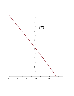
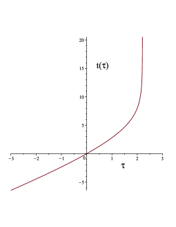
Figure 1: Numerical integration of the timelike ($\epsilon=1$ in Eq. (III)) geodesics in a 2-dimensional Schwarzschild spacetime, with parameters $M=1,E=3/2$ and initial conditions $r(0)=5,t(0)=0$. One sees (numerically) that when $\tau_{*}=2.2053644$ the particle has reached $r=2$ while $t(\tau_{*})\approx 38.3832$.

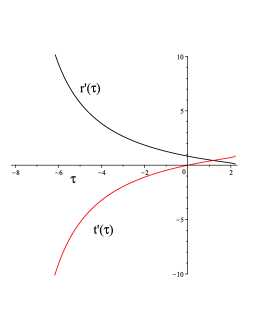
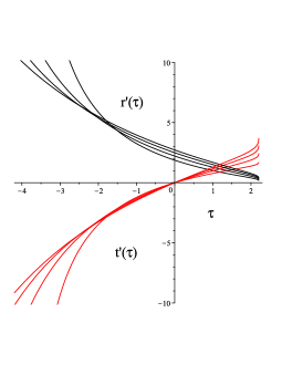
Figure 2: Upper panel: The orbit of Fig.1 is referred to the projective coordinates $r^{\prime}$ and $t^{\prime}$ obtained by using the values $A^{1}{}_{1}=A^{2}{}_{2}=A^{0}{}_{1}=A^{0}{}_{2}=1$ for the projection matrix, implying $r^{\prime}=r/(1+t+r)$ (black online) and $t^{\prime}=t/(1+t+r)$ (red online). However, upon continuing the plots up to $\tau\approx-8.30$ the functions $r^{\prime}(\tau)$ and $t^{\prime}(\tau)$ diverge, i.e., the map has a pole since we are moving along the geodesics. Similarly, one cannot extend the plots beyond the value $\tau=2.21$, at which both $t^{\prime},r^{\prime}$ reach their asymptotic values, in this case (and within the numerical precision of the plots) $r^{\prime}_{\rm asymt}=0.1079$, $t^{\prime}_{\rm asymt}=0.8384$ . Lower panel: Sequence of plots of $r^{\prime}=r/(1+A^{0}{}_{1}t+A^{0}{}_{2}r)$ (black online) and $t^{\prime}=t/(1+A^{0}{}_{1}t+A^{0}{}_{2}r)$ (red online) as in the upper panel but using different values for $[A^{0}{}_{1},A^{0}{}_{2}]=\{[\frac{1}{2},\frac{1}{3}],[\frac{1}{3},\frac{1}{4}],[\frac{1}{4},\frac{1}{5}],[\frac{1}{5},\frac{1}{6}]\}$. On the right of $\tau=2$, the numerical integration finds a vertical asymptote of $t^{\prime}(\tau)$.

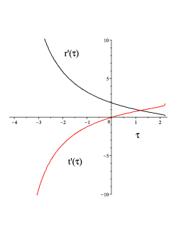
Figure 3: The lower panel of Fig. 2 repeated for $A^{0}{}_{1}=\frac{1}{2},A^{0}{}_{2}=\frac{1}{3}$. Such geodesics reach future timelike infinity, i.e., the point $(t^{\prime}=2,r^{\prime}=0)$.

III Points at infinity in 2-dimensional Schwarzschild spacetime

Let us first consider a 2-dimensional Schwarzschild spacetime with metric written in standard $x^{a}=(t,r)$ coordinates (we use $G=c=1$ units)

$$ds^{2}=-\left(1-\frac{2M}{r}\right)dt^{2}+\frac{dr^{2}}{\left(1-\frac{2M}{r}\right)}.$$ (40)

It is well known that

$$R_{ab}=\frac{2M}{r^{3}}g_{ab}\,,\qquad R=\frac{4M}{r^{3}},$$ (41)

i.e.,

$$G_{ab}=R_{ab}-\frac{1}{2}Rg_{ab}=0\,.$$ (42)

The geodesic equation reduces to

$$\frac{dt}{d\tau} = \frac{E}{1-\frac{2M}{r}},$$

$$\frac{dr}{d\tau} = \pm\sqrt{E^{2}-\epsilon\left(1-\frac{2M}{r}\right)},$$ (43)

where $E$ is the energy (Killing) constant and $\epsilon=[1,0,-1]$ for timelike, null and spacelike orbits, respectively.

We study the following fractional-linear coordinate transformation

$$t^{\prime} = \frac{A^{1}{}_{B}y^{B}}{A^{0}{}_{C}y^{C}}=\frac{A^{1}{}_{0}+A^{1}{}_{1}t+A^{1}{}_{2}r}{\rho},$$

$$r^{\prime} = \frac{A^{2}{}_{B}y^{B}}{A^{0}{}_{C}y^{C}}=\frac{A^{2}{}_{0}+A^{2}{}_{1}t+A^{2}{}_{2}r}{\rho},$$ (44)

where we have defined

$$\rho=A^{0}{}_{0}+A^{0}{}_{1}t+A^{0}{}_{2}r=A^{0}{}_{0}+A^{0}{}_{a}x^{a}.$$ (45)

We can express the differentials as follows:

$$dt^{\prime} = \left(\frac{A^{1}{}_{1}}{\rho}-A^{0}{}_{1}\frac{t^{\prime}}{\rho}\right)dt+\left(\frac{A^{1}{}_{2}}{\rho}-A^{0}{}_{2}\frac{t^{\prime}}{\rho}\right)dr,$$

$$dr^{\prime} = \left(\frac{A^{2}{}_{1}}{\rho}-A^{0}{}_{1}\frac{r^{\prime}}{\rho}\right)dt+\left(\frac{A^{2}{}_{2}}{\rho}-A^{0}{}_{2}\frac{r^{\prime}}{\rho}\right)dr,\qquad$$ (46)

implying (concisely, since there is no need to write lengthy expressions explicitly)

$$dt = B^{t}{}_{t^{\prime}}dt^{\prime}+B^{t}{}_{r^{\prime}}dr^{\prime},$$

$$dr = B^{r}{}_{t^{\prime}}dt^{\prime}+B^{r}{}_{r^{\prime}}dr^{\prime},$$ (47)

and then leading to the new form of the metric

$$ds^{2} = g_{t^{\prime}t^{\prime}}dt^{\prime}{}^{2}+2g_{t^{\prime}r^{\prime}}dt^{\prime}dr^{\prime}+g_{r^{\prime}r^{\prime}}dr^{\prime}{}^{2}.$$ (48)

In order to bring infinity down to a finite distance, the choice of $A$ for which

$$A^{0}{}_{1}\not=0,\qquad A^{1}{}_{1}\not=0,$$ (49)

$$A^{0}{}_{2}\not=0,\qquad A^{2}{}_{2}\not=0,$$ (50)

is of particular interest, because such equations ensure that $t\to\infty$ corresponds to

$${A^{1}{}_{1}\over A^{0}{}_{1}}=\lim_{t\to\ \infty}t^{\prime}$$ (51)

at finite values of $r$, and $r=+\infty$ corresponds to

$${A^{2}{}_{2}\over A^{0}{}_{2}}=\lim_{r\to\infty}r^{\prime}$$ (52)

at finite values of $t$, respectively.

Note that in the Eqs. (44) and (45) one has to choose special values of the coefficients $A^{\alpha}{}_{\beta}$. As a first example, let us consider the numerical integration of the timelike geodesics in a 2-dimensional Schwarzschild spacetime, examining the radial infalling orbits.

Besides the standard $(t,r)$ coordinates of the metric (40), one can describe the radial motion through the projective coordinates defined above. As in Sec. II, we use the simple choice of $A^{B}{}_{B}=1$, $A^{0}{}_{1}$ and $A^{0}{}_{2}$ as only nonvanishing coefficients, implying

$$t^{\prime}=\frac{t}{\rho},\qquad r^{\prime}=\frac{r}{\rho},$$ (53)

with $\rho=1+tA^{0}{}_{1}+rA^{0}{}_{2}$. We have then (explicitly, in this special case)

$$dt^{\prime} = \frac{1}{\rho}\left(1-\frac{tA^{0}{}_{1}}{\rho}\right)dt-\frac{t}{\rho^{2}}A^{0}{}_{2}dr,$$

$$dr^{\prime} = -\frac{r}{\rho^{2}}A^{0}{}_{1}dt+\frac{1}{\rho}\left(1-\frac{rA^{0}{}_{2}}{\rho}\right)dr,$$ (54)

with inverse relations (identifying the coefficients $B^{i}{}_{j}$ of Eq. (47))

$$dt = \rho^{2}(-r^{\prime}A^{0}{}_{2}+1)dt^{\prime}+\rho^{2}t^{\prime}A^{0}{}_{2}dr^{\prime},$$

$$dr = \rho^{2}r^{\prime}A^{0}{}_{1}dt^{\prime}+\rho^{2}(-t^{\prime}A^{0}{}_{1}+1)dr^{\prime},$$ (55)

and the new metric (48) given by

$$g_{t^{\prime}t^{\prime}} = -\frac{\rho^{3}(\rho r^{\prime}-2M)(r^{\prime}A^{0}{}_{2}-1)^{2}}{r^{\prime}}+\frac{\rho^{5}r^{\prime}{}^{3}(A^{0}{}_{1})^{2}}{(\rho r^{\prime}-2M)},$$

$$g_{t^{\prime}r^{\prime}} = \frac{(\rho r^{\prime}-2M)\rho^{3}(r^{\prime}A^{0}{}_{2}-1)t^{\prime}A^{0}{}_{2}}{r^{\prime}}$$

$$-\frac{r^{\prime}{}^{2}A^{0}{}_{1}(t^{\prime}A^{0}{}_{1}-1)\rho^{5}}{(\rho r^{\prime}-2M)},$$

$$g_{r^{\prime}r^{\prime}} = -\frac{(\rho r^{\prime}-2M)\rho^{3}t^{\prime}{}^{2}(A^{0}{}_{2})^{2}}{r^{\prime}}$$ (56)

$$+\frac{\rho^{5}(t^{\prime}A^{0}{}_{1}-1)^{2}r^{\prime}}{(\rho r^{\prime}-2M)}.$$

With a simple choice of parameters and initial conditions the numerical integration of the geodesics with $(t,r)$ coordinates is summarized in Fig. 1. Figure 2 offers instead the picture of the same geodesic orbit but with the projective coordinates $(t^{\prime},r^{\prime})$. We have chosen therein rational values of $A_{\;1}^{0}$ and $A_{\;2}^{0}$ so that, by virtue of (51) and (52), timelike and spacelike infinity read as

$$(2,0),(3,0),...,(0,3),(0,4),...$$

respectively.

For this simple example we can consider the observers adapted to the projective coordinates, Eq. (32). They form a congruence of accelerated worldlines, with nonzero expansion but vanishing vorticity. The use of such observers as fiducial observers will anyway complicate matters. For example, together with

$$u_{\rm pc}=\frac{1}{\sqrt{-g_{t^{\prime}t^{\prime}}}}\frac{\partial}{\partial t^{\prime}}$$ (57)

one has the orthogonal direction

$$e(u_{\rm pc})_{1}=Z_{1}\left[g_{r^{\prime}t^{\prime}}\frac{\partial}{\partial t^{\prime}}-g_{t^{\prime}t^{\prime}}\frac{\partial}{\partial r^{\prime}}\right]$$ (58)

with $Z_{1}$ obtained from the normalization condition,

$$Z_{1}=\frac{1}{\sqrt{-g_{t^{\prime}t^{\prime}}}\sqrt{(g_{r^{\prime}t^{\prime}})^{2}-g_{t^{\prime}t^{\prime}}g_{r^{\prime}r^{\prime}}}}.$$ (59)

The acceleration of $u_{\rm pc}$ is then

$$a(u_{\rm pc})=\nabla_{u_{\rm pc}}u_{\rm pc}=\kappa e(u_{\rm pc})_{1}.$$ (60)

Here $\kappa$ is a complicated function of $t^{\prime}$ and $r^{\prime}$. For example, for $A^{0}{}_{1}=1$, $A^{0}{}_{2}=0$ we find

$$\kappa^{2}=M^{2}\frac{(1-t^{\prime})^{4}Z_{3}(Z_{2})^{2}}{r^{\prime}{}^{3}(Z_{3}^{2}-r^{\prime}{}^{4})^{3}},$$ (61)

where

$$Z_{3}=r^{\prime}+2M(t^{\prime}-1),\;Z_{2}=-3r^{\prime}{}^{4}+Z_{1}^{2}.$$ (62)

Figure 4: Timelike equatorial plane geodesics of a four-dimensional Scwarzschild spacetime mapped into projective coordinates. $t^{\prime}=t/(1+A^{0}{}_{1}t+A^{0}{}_{2}r)$ (red online), $r^{\prime}=r/(1+A^{0}{}_{1}t+A^{0}{}_{2}r)$ (black online) $\theta^{\prime}=\pi/2(1+A^{0}{}_{1}t+A^{0}{}_{2}r)$ (grey online) $\phi^{\prime}=\phi/(1+A^{0}{}_{1}t+A^{0}{}_{2}r)$ (blue online). The original Schwarzschild geodesics are radially outgoing with parameters $M=1$,$E=2$ (energy per unit of mass), $L=2$ (angular momentum per unit of mass) following the initial conditions $\phi(0)=0,r(0)=5,t(0)=0$. The projective parameters chosen are $[A^{0}{}_{1},A^{0}{}_{2}]=[\frac{1}{2},\frac{1}{3}]$. From this figure we find that timelike geodesics do not reach our future projective infinity $(2,0,0,0)$, and the same holds for past timelike infinity $(-2,0,0,0)$. This projective picture is relevant, for example, for all timelike geodesics which describe the motion of planets about the Sun. The same qualitative behavior is obtained on considering other choices of $A_{\;1}^{0}$ and $A_{\;2}^{0}$, as well as on studying the projective version of null geodesics. Thus, we have avoided displaying multiple figures with the same content.

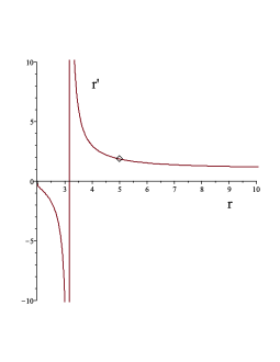
Figure 5: By using the same parameters and initial conditions of Fig. 4 we display the behavior of $r^{\prime}$ vs $r$, with $\tau$ as the parametric plot parameter. The highlighted point corresponds to the value $\tau=0$ ($r=5,r^{\prime}=1.875$). The numerically evaluated asymptotic value of $r^{\prime}$ is $r^{\prime}(10^{6})=1.0981$.

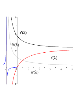
Figure 6: By using the same parameters and initial conditions of Fig. 4 we display the behavior of the null equatorial plane geodesics as functions of an affine parameter $\lambda$.

IV Second look at points at infinity in Schwarzschild spacetime

In order to further test the suggestion made in Eqs. (5)-(7), we here consider the standard $(t,r,\theta,\phi)$ coordinates for Schwarzschild geometry, for which, upon exploiting a ${\rm GL}(5,{\mathbb{R}})$ matrix with components $A_{\;C}^{B}$, we pass to new coordinates

$$t^{\prime} = \frac{T}{\rho},\qquad r^{\prime}=\frac{R}{\rho},$$

$$\theta^{\prime} = \frac{\Theta}{\rho}\,,\qquad\phi^{\prime}=\frac{\Phi}{\rho},$$ (63)

where

$$T(t,r,\theta,\phi) = A^{1}{}_{0}+A^{1}{}_{\alpha}x^{\alpha}$$

$$R(t,r,\theta,\phi) = A^{2}{}_{0}+A^{2}{}_{\alpha}x^{\alpha}$$

$$\Theta(t,r,\theta,\phi) = A^{3}{}_{0}+A^{3}{}_{\alpha}x^{\alpha}$$

$$\Phi(t,r,\theta,\phi) = A^{4}{}_{0}+A^{4}{}_{\alpha}x^{\alpha},$$ (64)

with

$$\rho(t,r,\theta,\phi) = {{y^{\prime}}^{0}\over y^{0}}=\sum_{\nu=0}^{4}A^{0}{}_{\nu}{y^{\nu}\over y^{0}}$$ (65)

$$= A^{0}{}_{0}+A^{0}{}_{\alpha}x^{\alpha}.$$

Hereafter, we assume the form (12) for the matrix $A$ for the reasons described in Sec. II, and hence we find

$$dt^{\prime} = \frac{1}{\rho}\left(1-\frac{A_{\;1}^{0}t}{\rho}\right)dt-\frac{A_{\;2}^{0}t}{\rho^{2}}dr,$$

$$dr^{\prime} = -\frac{A_{\;1}^{0}r}{\rho^{2}}dt+\frac{1}{\rho}\left(1-\frac{A_{\;2}^{0}r}{\rho}\right)dr,$$

$$d\theta^{\prime} = -\frac{A_{\;1}^{0}\theta}{\rho^{2}}dt-\frac{A_{\;2}^{0}\theta}{\rho^{2}}dr+\frac{1}{\rho}d\theta,$$

$$d\phi^{\prime} = -\frac{A_{\;1}^{0}\phi}{\rho^{2}}dt-\frac{A_{\;2}^{0}\phi}{\rho^{2}}dr+\frac{1}{\rho}d\phi.$$ (66)

At this stage, we solve the system (66) for $dt,dr,d\theta$ and $d\phi$ in the form

$$dx^{\mu}=B^{\mu}{}_{\nu}(x^{\prime})d{x^{\prime}}^{\nu},$$ (67)

bearing in mind that

$$t=\rho t^{\prime},\;r=\rho r^{\prime},\;\theta=\rho\theta^{\prime},\;\phi=\rho\phi^{\prime},$$ (68)

while $\rho$ obeys the equation

$$\rho=1+A_{\;1}^{0}t+A_{\;2}^{0}r=1+\rho(A_{\;1}^{0}t^{\prime}+A_{\;2}^{0}r^{\prime}),$$ (69)

which is solved by

$$\rho=\left(1-A_{\;1}^{0}t^{\prime}-A_{\;2}^{0}r^{\prime}\right)^{-1}=\rho(t^{\prime},r^{\prime}).$$ (70)

Hence we find that the metric has nondiagonal form in the $(t^{\prime},r^{\prime},\theta^{\prime},\phi^{\prime})$ coordinates:

$$g_{t^{\prime}t^{\prime}} = \frac{\rho^{3}}{r^{\prime}}F(r^{\prime}A^{0}{}_{2}-1)^{2}-\frac{r^{\prime}{}^{3}\rho^{5}\Bigr{(}A_{\;1}^{0}\Bigr{)}^{2}}{F}+\Bigr{(}A_{\;1}^{0}\Bigr{)}^{2}\rho^{6}r^{\prime}{}^{2}\Omega^{\prime}$$

$$g_{r^{\prime}r^{\prime}} = \frac{\rho^{3}}{r^{\prime}}Ft^{\prime}{}^{2}\Bigr{(}A_{\;2}^{0}\Bigr{)}^{2}-\frac{r^{\prime}\rho^{5}(-t^{\prime}A^{0}{}_{1}+1)^{2}}{F}+\Bigr{(}A_{\;2}^{0}\Bigr{)}^{2}\rho^{6}r^{\prime}{}^{2}\Omega^{\prime}$$

$$g_{\theta^{\prime}\theta^{\prime}} = r^{\prime}{}^{2}\rho^{4}$$

$$g_{\phi^{\prime}\phi^{\prime}} = \rho^{4}{\mathcal{R}}^{2}$$

$$g_{t^{\prime}r^{\prime}} = -\frac{\rho^{3}}{r^{\prime}}F(r^{\prime}A^{0}{}_{2}-1)t^{\prime}A^{0}{}_{2}-\frac{r^{\prime}{}^{2}\rho^{5}A^{0}{}_{1}(-t^{\prime}A^{0}{}_{1}+1)}{F}+A^{0}{}_{1}A^{0}{}_{2}\rho^{6}r^{\prime}{}^{2}\Omega^{\prime}$$

$$g_{t^{\prime}\theta^{\prime}} = r^{\prime}{}^{2}A^{0}{}_{1}\theta^{\prime}\rho^{5}$$

$$g_{t^{\prime}\phi^{\prime}} = \rho^{5}{\mathcal{R}}^{2}\phi^{\prime}A^{0}{}_{1}$$

$$g_{r^{\prime}\theta^{\prime}} = r^{\prime}{}^{2}\rho^{5}\theta^{\prime}A^{0}{}_{2}$$

$$g_{r^{\prime}\phi^{\prime}} = \rho^{5}{\mathcal{R}}^{2}\phi^{\prime}A^{0}{}_{2}$$

$$g_{\theta^{\prime}\phi^{\prime}} = 0,$$ (71)

where

$$\Omega^{\prime}=\sin^{2}(\theta^{\prime}\rho)\phi^{\prime}{}^{2}+\theta^{\prime}{}^{2},\qquad F=2M-r^{\prime}\rho,\qquad{\mathcal{R}}^{2}=r^{\prime}{}^{2}\sin^{2}(\theta^{\prime}\rho).$$ (72)

This is a particular case of the spherically symmetric metric with inhomogeneous projective coordinates obtained by us in Appendix B. We now display the projective version of timelike and null geodesics by using Eq. (13), and then using for $t,r,\theta,\phi$ on the right-hand side therein the formulas obtained in Ref. Chandra , limiting to equatorial plane $\theta=\pi/2$ geodesics without any loss of generality.

V Nariai spacetime

We now consider the Nariai spacetime model Nariai1 ; Nariai2 which is of particular interest because for it the Penrose conformal boundary cannot be defined. Following Ref. Kroon one can point out that, if a solution of the Einstein equations admits a smooth conformal extension, then the conformally rescaled Weyl tensor should satisfy the condition

$${\widetilde{C}}_{\lambda\mu\nu\rho}{\widetilde{C}}^{\lambda\mu\nu\rho}=0.$$

But in the Nariai case, one finds

$${\widetilde{C}}_{\lambda\mu\nu\rho}{\widetilde{C}}^{\lambda\mu\nu\rho}={\rm constant}\;\not=0.$$

This contradicts the above condition, and hence there cannot exist a piece of conformal boundary which is of class $C^{2}$ Kroon .

The Nariai spacetime metric Nariai1 ; Nariai2 written in dimensionless spherical-like coordinates $(t,r,\theta,\phi)$ reads as

$$ds^{2}=-dt^{2}+\cosh^{2}t\,dr^{2}+d\theta^{2}+\sin^{2}\theta d\phi^{2},$$ (73)

and is an exact solution of Einstein’s field equation with cosmological constant $\Lambda=-1$, i.e., with

$$G_{\alpha\beta}=g_{\alpha\beta}.$$ (74)

It has several important properties Kroon :

1. geodesic completeness Beyer ;

2. globally hyperbolicity;

3. it does not even admit a patch of a conformal boundary;

4. it is algebraically special of Petrov type D.

The $t-r$ part of the metric

$$ds_{(t,r)}^{2}=-dt^{2}+\cosh^{2}t\,dr^{2}\,,$$ (75)

can be used to visualize the modifications to the light cones as time evolves. For instance, looking at the family of points $(r_{0},t_{0})$ with $r_{0}$ fixed and $t_{0}$ taken as a parameter, the light-cone equation becomes

$$t-t_{0}=\pm(\cosh t_{0})(r-r_{0}).$$ (76)

This relation leads to the $45$ degree opening angle at $t_{0}=0$, and then the angle gets restricted continuously, vanishing in the limit $t_{0}\to\infty$. Differently, with $t_{0}$ fixed and $r_{0}$ taken as a parameter, the light-cone structure is fixed itself, i.e., the opening angle does not depend on $r_{0}$.

The spherical-like coordinates are adapted to the two Killing vector fields

$$\frac{\partial}{\partial r},\qquad\frac{\partial}{\partial\phi}.$$ (77)

The existence of these Killing symmetries makes it possible to separate the geodesics. On denoting their parametric equations by $x^{\alpha}=x^{\alpha}(\tau)$, one has

$$\frac{dt}{d\tau} = \sqrt{C_{2}+\frac{C_{1}^{2}}{\cosh^{2}t}},$$

$$\frac{dr}{d\tau} = \frac{C_{1}}{\cosh^{2}t}\,,$$

$$\frac{d\theta}{d\tau} = \pm\sqrt{C_{3}-\frac{L^{2}}{\sin^{2}\theta}},$$

$$\frac{d\phi}{d\tau} = \frac{L}{\sin^{2}\theta},$$ (78)

where the $C_{i}$ and $L$ are constant and we have chosen $dt/d\tau>0$ to have future-oriented orbits. Interestingly, these equations are pairwise coupled, i.e., the coupled variables are $(t,r)$ (corresponding to geodesic motion on the pseudosphere) and $(\theta,\phi)$ (corresponding to geodesic motion on the $2$-sphere), with no mutual intersections. For instance, by assuming $L=0$ and $C_{3}=0$ one has $\theta(\tau)=\theta(0)$, $\phi(\tau)=\phi(0)$ and one is left with the temporal and radial equations only. The normalization condition for these orbits: $U\cdot U=-\epsilon$, with $U^{\alpha}=\frac{dx^{\alpha}}{d\tau}$ and $\epsilon=[1,0,-1]$ for timelike, null, spacelike orbits, respectively, reads as

$$-\left(\frac{dt}{d\tau}\right)^{2}+\left(\frac{d\theta}{d\tau}\right)^{2}+\frac{C_{1}^{2}}{\cosh^{2}t}+\frac{L^{2}}{\sin^{2}\theta}+\epsilon=0,$$ (79)

where only the Killing relations have been used. Inserting in Eq. (79) the full set of Eqs. (78) one finds

$$C_{2}=C_{3}+\epsilon,$$ (80)

meaning that, once a causality condition is imposed, the integration constants $C_{2}$ and $C_{3}$ are no longer freely specifiable.

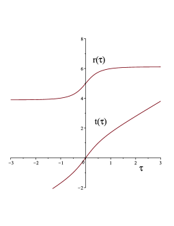
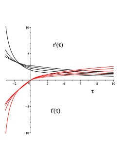
Figure 7: Upper panel: Example of numerical integration of the timelike geodesics in the Nariai spacetime with parameters $C_{1}=2,C_{2}=1,C_{3}=0,L=0$ and initial conditions $\phi(0)=0,r(0)=5,t(0)=0,\theta(0)=\frac{\pi}{4}$. Lower panel: The same map as in Fig. 2 (lower panel), i.e., $r^{\prime}=r/(1+A^{0}{}_{1}t+A^{0}{}_{2})$ (black online) and $t^{\prime}=t/(1+A^{0}{}_{1}t+A^{0}{}_{2})$ (red online), using different values for $[A^{0}{}_{1},A^{0}{}_{2}]=\{[\frac{1}{2},\frac{1}{3}],[\frac{1}{3},\frac{1}{4}],[\frac{1}{4},\frac{1}{5}],[\frac{1}{5},\frac{1}{6}]\}$.

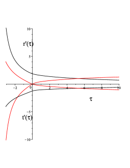
Figure 8: Fig. 7 (lower panel) repeated by using for $A^{0}{}_{1}=\frac{1}{n},A^{0}{}_{2}=\frac{1}{(n+1)}$ for $n=2,-2$.

A natural orthonormal frame is the following:

$$e_{0} = \frac{\partial}{\partial t},\qquad e_{1}=\frac{1}{\cosh t}\frac{\partial}{\partial r},$$

$$e_{2} = \frac{\partial}{\partial\theta},\qquad e_{3}=\frac{1}{\sin\theta}\frac{\partial}{\partial\phi},$$ (81)

which can be used to form a standard Newman-Penrose frame

$$l = \frac{1}{\sqrt{2}}(e_{0}+e_{2})\,,\qquad n=\frac{1}{\sqrt{2}}(e_{0}-e_{2}),$$

$$m = \frac{1}{\sqrt{2}}(e_{1}+ie_{3}).$$ (82)

The non-vanishing spin coefficients reduce to

$$\sigma = -\mu=\frac{\sqrt{2}}{4}\left(-\tanh t+\cot\theta\right)\,,$$

$$\lambda = -\rho=\frac{\sqrt{2}}{4}\left(\tanh t+\cot\theta\right).$$ (83)

The non-vanishing Weyl scalars are all constant:

$$\psi_{0}=\psi_{4}=-\frac{1}{2}\,,\qquad\psi_{2}=\frac{1}{6},$$ (84)

from which the algebraically special nature of this metric follows easily.

By virtue of Eq. (73), we can use the same coordinates of Sec. II in order to define three concepts of projective infinity. The isolated points pertaining to future timelike infinity, spacelike infinity and past timelike infinity arise from a projective map which engenders destruction of the $2$-sphere, whereas future and past null infinity arise from a projective map which preserves the $2$-sphere.

On passing to new coordinates

$$t^{\prime} = \frac{T}{\rho}\,,\qquad r^{\prime}=\frac{R}{\rho},$$

$$\theta^{\prime} = \frac{\Theta}{\rho},\qquad\phi^{\prime}=\frac{\Phi}{\rho},$$ (85)

where $\rho=1+A^{0}{}_{1}t+A^{0}{}_{2}r$, the metric transforms as follows (cf. Appendix B):

$$g_{t^{\prime}t^{\prime}} = -\rho^{4}(r^{\prime}A^{0}{}_{2}-1)^{2}+\rho^{4}r^{\prime}{}^{2}\Bigr{(}A_{\;1}^{0}\Bigr{)}^{2}\cosh^{2}(t^{\prime}\rho)+\Bigr{(}A_{\;1}^{0}\Bigr{)}^{2}\rho^{4}[\theta^{\prime}{}^{2}+\sin^{2}(\theta^{\prime}\rho)\phi^{\prime}{}^{2}]$$

$$g_{r^{\prime}r^{\prime}} = -\rho^{4}t^{\prime}{}^{2}\Bigr{(}A_{\;2}^{0}\Bigr{)}^{2}+\rho^{4}(-t^{\prime}A^{0}{}_{1}+1)^{2}\cosh^{2}(t^{\prime}\rho)+\Bigr{(}A_{\;2}^{0}\Bigr{)}^{2}\rho^{4}[\theta^{\prime}{}^{2}+\sin^{2}(\theta^{\prime}\rho)\phi^{\prime}{}^{2}]$$

$$g_{\theta^{\prime}\theta^{\prime}} = \rho^{2}$$

$$g_{\phi^{\prime}\phi^{\prime}} = \rho^{2}\sin^{2}(\theta^{\prime}\rho)$$

$$g_{t^{\prime}r^{\prime}} = \rho^{4}(r^{\prime}A^{0}{}_{2}-1)t^{\prime}A^{0}{}_{2}+\rho^{4}r^{\prime}A^{0}{}_{1}(-t^{\prime}A^{0}{}_{1}+1)\cosh^{2}(t^{\prime}\rho)+A^{0}{}_{1}A^{0}{}_{2}\rho^{4}[\theta^{\prime}{}^{2}+\sin^{2}(\theta^{\prime}\rho)\phi^{\prime}{}^{2}]$$

$$g_{t^{\prime}\theta^{\prime}} = \rho^{3}\theta^{\prime}A^{0}{}_{1}$$

$$g_{t^{\prime}\phi^{\prime}} = \rho^{3}\sin^{2}(\theta^{\prime}\rho)\phi^{\prime}A^{0}{}_{1}$$

$$g_{r^{\prime}\theta^{\prime}} = \rho^{3}\theta^{\prime}A^{0}{}_{2}$$

$$g_{r^{\prime}\phi^{\prime}} = \rho^{3}\sin^{2}(\theta^{\prime}\rho)\phi^{\prime}A^{0}{}_{2}$$

$$g_{\theta^{\prime}\phi^{\prime}} = 0.$$ (86)

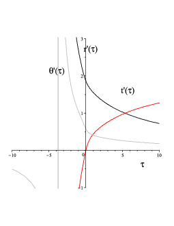
Figure 9: Timelike equatorial plane geodesics of a Nariai spacetime mapped into projective coordinates. The parameter and initial conditions choices are the same as in Fig. 7. These values imply $\phi(\tau)\equiv 0$ and then it is not included in the plot. The projective parameters chosen are $[A^{0}{}_{1},A^{0}{}_{2}]=[\frac{1}{2},\frac{1}{3}]$. The numerical integration gives the following asymptotic values: $r^{\prime}(10^{6})=1.2\cdot 10^{-5}$, $t^{\prime}(10^{6})=2.00$, $\theta^{\prime}(10^{6})=3.14\cdot 10^{-6}$. Thus, within the numerical approximation we see that timelike geodesics reach our future projective infinity $(2,0,0,0)$. The same qualitative behavior is obtained on considering other choices of $A_{\;1}^{0}$ and $A_{\;2}^{0}$.

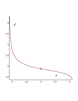
Figure 10: By using the same parameters and initial conditions of Fig. 9 we display the behavior of $r^{\prime}$ vs $r$, with $\tau$ as the parametric plot parameter. The highlighted point corresponds to the value $\tau=0$.

VI Points at the boundary of the accessible region in a de Sitter spacetime

Consider de Sitter spacetime, whose line element written in spherical-like coordinates is given by

$$ds^{2}=-N^{2}dt^{2}+\frac{dr^{2}}{N^{2}}+r^{2}(d\theta^{2}+\sin^{2}\theta d\phi^{2}),$$ (87)

where $N=(1-H^{2}r^{2})^{1/2}$ denotes the “lapse” function. The spacetime region which can be accessed is the ball of radius $r_{b}=1/H$ and center at the origin. When examining any kind of motion in this spacetime the radial (compact) region $r\in[0,\frac{1}{H}]$ is the only one which has to be explored. By virtue of the simplicity of the metric, with $G_{\alpha\beta}=-3H^{2}g_{\alpha\beta}$, the geodesics are integrable as a first order system of equations

$$\frac{dt}{d\tau} = \frac{E^{2}}{N^{2}},$$

$$\frac{d\phi}{d\tau} = \frac{L}{r^{2}\sin^{2}\theta},$$

$$\frac{d\theta}{d\tau} = \frac{\epsilon_{\theta}}{r^{2}}\sqrt{C-\frac{L^{2}}{\sin^{2}\theta}},$$

$$\frac{dr}{d\tau} = \frac{\epsilon_{r}}{r}\sqrt{E^{2}+(\epsilon r^{2}+C^{2})(H^{2}r^{2}-1)},$$ (88)

where $E$ and $L$ are Killing constants, $\epsilon=[1,0,-1]$ for timelike, null, spacelike orbits, respectively, $C$ is a separation constant for radial-polar motions and $\epsilon_{r},\epsilon_{\theta}$ are two independent signs. Equatorial plane motion, $\theta=\pi/2$, corresponds to $C=L$ and the above equations take the simpler form

$$\frac{dt}{d\tau} = \frac{E^{2}}{N^{2}},$$

$$\frac{d\phi}{d\tau} = \frac{L}{r^{2}},$$

$$\frac{dr}{d\tau} = \frac{\epsilon_{r}}{r}\sqrt{E^{2}+(\epsilon r^{2}+L^{2})(H^{2}r^{2}-1)}.$$ (89)

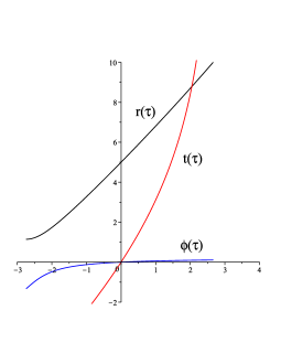
Figure 11: Numerical integration of timelike geodesics in standard spherical coordinates. The parameter values are $H_{0}=\frac{1}{10}$, $E=2$, $L=2$, while initial conditions are $r(0)=5$, $t(0)=0$, $\phi(0)=0$.

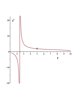
Figure 12: By using the same parameters and initial conditions of Fig. 11 we display the behavior of $r^{\prime}$ vs $r$, with $\tau$ as the parametric plot parameter. The highlighted point corresponds to the value $\tau=0$.

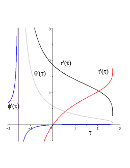
Figure 13: Timelike equatorial plane geodesics of a de sitter spacetime mapped into projective coordinates. The parameter and initial conditions choices are the same as in Fig. 11. The projective parameters chosen are $[A^{0}{}_{1},A^{0}{}_{2}]=[\frac{1}{2},\frac{1}{3}]$. The maximal value of $\tau$ allowed for the numerical integration is $\tau_{\rm max}=2.6611$, such that $r^{\prime}(\tau_{\rm max})=0.1910$, $t^{\prime}(\tau_{\rm max})=1.8344$, $\theta^{\prime}(\tau_{\rm max})=0.0300$, $\phi^{\prime}(\tau_{\rm max})=0.0021$.

As far as we can see from Fig. $13$, timelike geodesics reach future timelike infinity $(2,0,0,0)$, up to the limitations resulting from numerical integration, whereas spacelike infinity $(0,3,0,0)$ seems to be inaccessible.

VII Concluding remarks

According to the method developed in our paper for dealing with points at infinity, we first choose the symmetry of interest; second, local coordinates are chosen that are appropriate for such a case; third, such physical coordinates are regarded as if they were obtained by a set of homogeneous (but unphysical) projective coordinates $(y^{0},y^{1},y^{2},y^{3},y^{4})$. As far as we can see, the original contributions of our approach are therefore as follows. (i) We have shown that there exists a bijective correspondence between points of spacetime with local coordinates $(x^{1},...,x^{4})$ and points of real projective space $S_{4}$ with homogeneous projective coordinates

$$(y^{0},...,y^{4})\sim\mu(y^{0},...,y^{4})\;\forall\mu\in{\mathbb{R}}-\{0\}.$$

This yields viable coordinate transformations after removing suitable lines from the spacetime $(M^{\prime},g^{\prime})$, and makes it possible to bring infinity down to a finite distance. (ii) The three kinds of infinity arise from different implementations of one and the same concept, i.e., a projective map. Interestingly, timelike and spacelike infinity are found to result from projective maps which destroy the $2$-sphere, whereas the projective counterpart of null infinity is found to originate from projective maps which preserve the $2$-sphere. (iii) We can define points at infinity even in cases where the conformal boundary does not exist, as shown in Sec. V. (iv) We can study geodesics and observers in inhomogeneous projective coordinates in a neat way.

A naturally generalization of our work concerns the projective definition of infinity in other kinds of spacetime. For this purpose, we have considered Gödel’s spacetime. The Gödel metric Godel ; HE is given by

$$ds^{2}=\frac{2}{\omega^{2}}\Bigr{[}-dt^{2}+dr^{2}-(\sinh^{4}r-\sinh^{2}r)d\phi^{2}$$ (90)

$$+2\sqrt{2}\sinh^{2}rd\phi\;dt\Bigr{]}+dz^{2},$$

with coordinates

$$t\in]-\infty,\infty[,\;r\in[0,\infty[,\;\phi\in[0,2\pi],\;z\in]-\infty,\infty[\,,$$

and an observer horizon located at $r=\ln(1+\sqrt{2})=0.8814$. See Ref. HE for all details. We provide below plots similar to those considered in the various examples above showing that passing to cylindrically symmetric spacetimes is feasible.

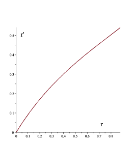
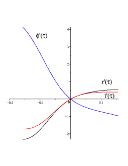
Figure 14: We display the behavior of $r^{\prime}$ vs $r$, with $\tau$ as the parametric plot parameter (upper panel) and the timelike geodesics on the $z=0$ plane (lower panel) in the Gödel spacetime. Spacetime and Killing parameters are chosen so that $E=20$, $L=0$, $\omega=1$, whereas the initial conditions are taken at the origin: $t(0)=0$, $r(0)=0$, $\phi(0)=0$. The projective map parameters are $A_{\;1}^{0}=\frac{1}{2}$, $A_{\;2}^{0}=\frac{1}{3}$, as usual.

Here we remark instead that, with a method analogous to the one in Sec. II, but relying now on a matrix $A\in{\rm GL}(4,{\mathbb{R}})$ having the form

$$A=\left(\begin{matrix}1&A_{\;1}^{0}&A_{\;2}^{0}&0\cr 0&1&0&0\cr 0&0&1&0\cr 0&0&0&1\end{matrix}\right),$$ (91)

we obtain the projective map

$$\frac{t^{\prime}}{t}=\frac{r^{\prime}}{r}=\frac{\phi^{\prime}}{\phi}=(1+A_{\;1}^{0}t+A_{\;2}^{0}r)^{-1},$$ (92)

which leads in turn to three kinds of projective infinity: (1) Timelike infinity, given by the point

$$\left(t^{\prime}=\frac{1}{A_{\;1}^{0}}={t^{\prime}}_{\infty},r^{\prime}=0,\phi^{\prime}=0\right).$$ (93)

Of course, the sign of $A_{\;1}^{0}$ may further distinguish among future and past timelike infinity. (2) Spacelike infinity, consisting of the point

$$\left(t^{\prime}=0,r^{\prime}=\frac{1}{A_{\;2}^{0}}={r^{\prime}}_{\infty},\phi^{\prime}=0\right).$$ (94)

(3) Direct product of half-lines in the first or fourth quadrant with $S^{1}$, whose points have coordinates

$$\left(t^{\prime}=t=-{t^{\prime}}_{\infty}\frac{r}{{r^{\prime}}_{\infty}},r^{\prime}=r,\phi^{\prime}=\phi\right).$$ (95)

In other words, when the projective map (92) destroys the $1$-sphere $S^{1}$, one deals with timelike or spacelike infinity, whereas if the projective map preserves the $1$-sphere, one obtains a two-dimensional manifold whose points have the coordinates in Eq. (95). As far as we can see from Fig. $14$, our future timelike infinity is not reached by geodesics in a Gödel universe.

Of course, a definition of infinity independent of any choice of symmetry with the associated coordinates is impossible within our framework. As far as we can see, no universal framework is conceivable. Carter-Penrose diagrams do not exist in all spacetimes, nor is null infinity always smooth in the standard approach Kehrberger . As is clear already from Secs. III and IV, our projective technique does not lead to a conformal rescaling of the original spacetime metric, and hence our definition of what we call projective counterpart of null infinity is not the boundary of the Penrose conformal completion of a physical spacetime (cf. the important work in Ref. AS ), and deserves further study. The application of our projective technique to the study of asymptotic properties of classical and quantum gravity is an important task in our opinion, in light of the huge amount of work in the recent literature (see, for example, Refs. Andy ; AE ; HT ; ME ). In the future it will be also interesting to understand whether any relation exists between the valuable work in Ref. Shabbir and our method.

Appendix A Projective coordinates

Let $r$ be the complex line supplemented by the point at infinity, and let $\lambda$ be a coordinate on $r$. If $S$ is a matrix of the group ${\rm GL}(2,\mathbb{C})$, written as

$$S=\left(\begin{matrix}a_{00}&a_{01}\cr a_{10}&a_{11}\end{matrix}\right),$$ (96)

the equation

$$\lambda^{\prime}=\frac{a_{11}\lambda+a_{10}}{a_{01}\lambda+a_{00}},$$ (97)

establishes a bijective correspondence, without exceptions, between $\lambda$ and $\lambda^{\prime}$, and $\lambda^{\prime}$ can be viewed as the new coordinate on $r$.

If $\lambda,\lambda^{\prime}$ are projective coordinates on the lines $r$ and $r^{\prime}$ respectively, Eq. (A2) establishes a correspondence $\omega:r\rightarrow r^{\prime}$ which is bijective without exceptions, and is called a projective correspondence.

Appendix B All metrics with spherical symmetry

Our Eqs. (66)-(66) can be inverted to express the differentials $dt,dr,d\theta,d\phi$. On defining

$$\alpha = \rho(1-A_{\;1}^{0}t^{\prime})^{-1}(1+\rho A_{\;1}^{0}A_{\;2}^{0}t^{\prime}r^{\prime}),$$

$$\beta = \rho^{2}A_{\;2}^{0}t^{\prime},$$

$$\gamma = \rho^{2}A_{\;1}^{0}r^{\prime},$$

$$\delta = \rho^{2}(1-A_{\;1}^{0}t^{\prime}),$$

$${\tilde{\alpha}} = \theta^{\prime}(A_{\;1}^{0}\alpha+A_{\;2}^{0}\gamma),$$

$${\tilde{\beta}} = \theta^{\prime}(A_{\;1}^{0}\beta+A_{\;2}^{0}\delta),$$

$${\tilde{\gamma}} = \phi^{\prime}(A_{\;1}^{0}\alpha+A_{\;2}^{0}\gamma),$$

$${\tilde{\delta}} = \phi^{\prime}(A_{\;1}^{0}\beta+A_{\;2}^{0}\delta),$$ (98)

we find

$$dt = \alpha\;dt^{\prime}+\beta\;dr^{\prime},$$

$$dr = \gamma\;dt^{\prime}+\delta\;dr^{\prime},$$

$$d\theta = {\tilde{\alpha}}\;dt^{\prime}+{\tilde{\beta}}\;dr^{\prime}+\rho\;d\theta^{\prime},$$

$$d\phi = {\tilde{\gamma}}\;dt^{\prime}+{\tilde{\delta}}\;dr^{\prime}+\rho\;d\phi^{\prime}.$$ (99)

Moreover, since

$$(1-A_{\;1}^{0}t^{\prime})^{-1}=\frac{\rho}{(1+\rho A_{\;2}^{0}r^{\prime})},$$ (100)

we obtain

$$A_{\;1}^{0}\alpha+A_{\;2}^{0}\gamma=\frac{\rho A_{\;1}^{0}(1+\rho A_{\;2}^{0}r^{\prime})}{(1-A_{\;1}^{0}t^{\prime})}=\rho^{2}A_{\;1}^{0},$$ (101)

while

$$A_{\;1}^{0}\beta+A_{\;2}^{0}\delta=\rho^{2}A_{\;2}^{0}.$$ (102)

By virtue of Eq. (101), we can solve for $\alpha$ in a more convenient form with respect to the first line of Eq. (98):

$$\alpha=\rho^{2}-\frac{A_{\;2}^{0}}{A_{\;1}^{0}}\gamma=\rho^{2}(1-A_{\;2}^{0}r^{\prime}).$$ (103)

In light of Eqs. (98)-(103), we can re-express any spherically symmetric metric

$$g=g_{tt}dt\otimes dt+g_{rr}dr\otimes dr+g_{\theta\theta}d\theta\otimes d\theta+g_{\phi\phi}d\phi\otimes d\phi,$$ (104)

in nondiagonal form, with components

$$g_{t^{\prime}t^{\prime}} = \rho^{4}\Bigr{[}g_{tt}(1-A_{\;2}^{0}r^{\prime})^{2}+g_{rr}(A_{\;1}^{0})^{2}{r^{\prime}}^{2}\Bigr{]}+\rho^{4}(A_{\;1}^{0})^{2}(g_{\theta\theta}{\theta^{\prime}}^{2}+g_{\phi\phi}{\phi^{\prime}}^{2}),$$

$$g_{t^{\prime}r^{\prime}} = \rho^{4}\Bigr{[}g_{tt}A_{\;2}^{0}(1-A_{\;2}^{0}r^{\prime})t^{\prime}+g_{rr}A_{\;1}^{0}r^{\prime}(1-A_{\;1}^{0}t^{\prime})\Bigr{]}+\rho^{4}A_{\;1}^{0}A_{\;2}^{0}(g_{\theta\theta}{\theta^{\prime}}^{2}+g_{\phi\phi}{\phi^{\prime}}^{2}),$$

$$g_{r^{\prime}r^{\prime}} = \rho^{4}\Bigr{[}g_{tt}(A_{\;2}^{0})^{2}{t^{\prime}}^{2}+g_{rr}(1-A_{\;1}^{0}t^{\prime})^{2}\Bigr{]}+\rho^{4}(A_{\;2}^{0})^{2}(g_{\theta\theta}{\theta^{\prime}}^{2}+g_{\phi\phi}{\phi^{\prime}}^{2}),$$

$$g_{t^{\prime}\theta^{\prime}} = g_{\theta\theta}\theta^{\prime}\rho^{3}A_{\;1}^{0},$$

$$g_{r^{\prime}\theta^{\prime}} = g_{\theta\theta}\theta^{\prime}\rho^{3}A_{\;2}^{0},$$

$$g_{t^{\prime}\phi^{\prime}} = g_{\phi\phi}\phi^{\prime}\rho^{3}A_{\;1}^{0},$$

$$g_{r^{\prime}\phi^{\prime}} = g_{\phi\phi}\phi^{\prime}\rho^{3}A_{\;2}^{0},$$

$$g_{\theta^{\prime}\theta^{\prime}} = g_{\theta\theta}\rho^{2},$$

$$g_{\phi^{\prime}\phi^{\prime}} = g_{\phi\phi}\rho^{2},$$

$$g_{\theta^{\prime}\phi^{\prime}} = 0.$$ (105)

References

(1)
S.W. Hawking, G.F.R. Ellis, The Large Scale Structure of Space-Time
(Cambridge University Press, Cambridge, 1973).
(2)
B.S. DeWitt, The Global Approach to Quantum Field Theory
(Oxford University Press, Oxford, 2003).
(3)
R. Penrose, Conformal treatment of infinity, in Relativity, Groups and Topology, 565-584, Eds.
C. DeWitt and B. DeWitt (Gordon and Breach, New York, 1964).
(4)
D. Eardley, R.K. Sachs, Space-times with a future projective
infinity, J. Math. Phys. 14, 209 (1973).
(5)
F. Severi, Lezioni sulle Funzioni Analitiche di più
Variabili Complesse (CEDAM, Padova, 1957).
(6)
H. Bondi, Spherically symmetrical models in general relativity,
Mon. Not. R. Astron. Soc. 107, 410 (1947).
(7)
B.G. Schmidt and J.M. Stewart, The scalar wave equation in
a Schwarzschild space-time, Proc. R. Soc. Lond. A 367,
503 (1979).
(8)
S. Chandrasekhar, The Mathematical Theory of Black Holes
(Oxford University Press, Oxford, 1983).
(9)
H. Nariai,
On some static solutions of Einstein’s gravitational field
equations in a spherically symmetric case,
Sci. Rep. Tohoku Univ. 34(3), 160-167 (1950).
(10)
H. Nariai,
On a new cosmological solution of Einstein’s field equations of gravitation,
Sci. Rep. Tohoku Univ. 35, 62-67 (1951).
(11)
J.A. Valiente Kroon, Conformal Methods in General Relativity
(Cambridge University Press, Cambridge, 2016).
(12)
F. Beyer, Non-genericity of the Nariai solutions: I. Asymptotics
and spatially homogeneous perturbations, Class. Quantum Grav.
26, 235015 (2009).
(13)
K. Gödel, An example of a new type of cosmological solutions
of Einstein’s field equations of gravitation,
Rev. Mod. Phys. 21, 447 (1949).
(14)
L.M.A. Kehrberger, The case against smooth null infinity I:
heuristics and counter-examples, Ann. H. Poincaré
23, 829 (2022).
(15)
A. Ashtekar, S. Speziale, Null infinity as a weakly isolated
horizon, arXiv:2402.17977 [hep-th].
(16)
A. Strominger, Lectures on the Infrared Structure of Gravity and
Gauge Theory (Princeton University Press, Princeton, 2017).
(17)
F. Alessio, G. Esposito, On the structure and applications of the
Bondi-Metzner-Sachs group, Int. J. Geom. Methods Mod. Phys.
15, 1830002 (2018).
(18)
M. Henneaux, C. Troessaert, BMS group at spatial infinity:
The Hamiltonian (ADM) approach, J. High Energy Phys.
2018, 3, 147 (2018).
(19)
Z. Mirzaiyan, G. Esposito, On the nature and applications of the
Bondi-Metzner-Sachs group, Symmetry 15, 947 (2023).
(20)
G. Shabbir, M.A. Qureshi, Proper projective symmetries in the
Schwarzschild metric, Mod. Phys. Lett. A 21, 1795 (2006).